The network uncertainty quantification method for
propagating uncertainties in component-based systems

Abstract

This work introduces the network uncertainty quantification (NetUQ) method for performing uncertainty propagation in systems composed of interconnected components. The method assumes the existence of a collection of components, each of which is characterized by exogenous-input random variables (e.g., material properties), endogenous-input random variables (e.g., boundary conditions defined by another component), output random variables (e.g., quantities of interest), and a local uncertainty-propagation operator (e.g., provided by stochastic collocation) that computes output random variables from input random variables. The method assembles the full-system network by connecting components, which is achieved simply by associating endogenous-input random variables for each component with output random variables from other components; no other inter-component compatibility conditions are required. The network uncertainty-propagation problem is: Compute output random variables for all components given all exogenous-input random variables. To solve this problem, the method applies classical relaxation methods (i.e., Jacobi and Gauss–Seidel iteration with Anderson acceleration), which require only black-box evaluations of component uncertainty-propagation operators. Compared with other available methods, this approach is applicable to any network topology (e.g., no restriction to feed-forward or two-component networks), promotes component independence by enabling components to employ tailored uncertainty-propagation operators, supports general functional representations of random variables, and requires no offline preprocessing stage. Also, because the method propagates functional representations of random variables throughout the network (and not, e.g., probability density functions), the joint distribution of any set of random variables throughout the network can be estimated a posteriori in a straightforward manner. We perform supporting convergence and error analysis and execute numerical experiments that demonstrate the weak- and strong-scaling performance of the method.

35R60, 60H15, 60H35, 65C20, 49M20, 49M27, 65N55

1 Introduction

Many systems in science and engineering—ranging from power grids to gas transfer systems to aircraft—comprise a collection of a large number of interconnected components. Performing uncertainty propagation in these systems is often essential for quantifying the influence of uncertainties on the performance of the full system. Naïvely, performing full-system uncertainty propagation in this context requires (1) integrating all component models into a single deterministic full-system model, and (2) executing uncertainty propagation using the deterministic full-system model. The first step is often challenging or impossible, as components are often characterized by vastly different physical phenomena and spatiotemporal scales, ensuring compatibility between the meshes of neighboring components is difficult, and components are often modeled using different simulation codes that can be difficult to integrate. If the first step is achievable, then the second step may still pose an insurmountable challenge due to the large-scale nature of the deterministic full-system model.

To address these challenges, researchers have developed several classes of methods that aim to decompose the full-system uncertainty-propagation problem into tractable subproblems. Ideally, such a method should satisfy several desiderata. First, the method should promote component independence. For example, each component should be able to use a tailored uncertainty-propagation method, as it has been shown that different uncertainty-propagation methods are better suited for different physics (see, e.g., Ref. [constantine2009hybrid]); in addition, the approach should avoid any coupled-component deterministic solves. Second, to be widely applicable, the method should not be restricted to systems with particular component-network topologies, as systems often comprise complex assemblies of components with two-way coupling between neighboring components. Third, the method should characterize uncertainties using functional representations of random variables, and should not be restricted to particular functional representations. Characterizing random variables using functional representations (i.e., as functions acting on the sample space) allows for the joint distribution of any set of random variables throughout the system to be estimated straightforwardly, and also facilitates other post-processing activities (e.g., variance-based decomposition). Supporting general representations is also important, as techniques restricted to polynomial-chaos representations [ghanem2003stochastic, xiu2002wiener], for example, are not compatible with other widely used random-variable representations [wan2006multi, bilionis2012multi, bilionis2012multidimensional].

The first class of methods replaces component high-fidelity models with component surrogate models, and subsequently computes inexpensive full-system samples either by propagating deterministic samples within a feed-forward network [martin2006methodology, sanson2018uncertainty], or by using domain-decomposition methods to converge these full-system samples [liao2015domain]. We point out that while these methods can significantly reduce the computational cost of full-system uncertainty propagation, they do not decompose the uncertainty-propagation task itself; thus, these methods do not enable each component to use a tailored uncertainty-propagation method. Relatedly, Ref. [friedman2018efficient] generates a surrogate model for the coupling variables across the system to facilitate generating full-system samples; however, this approach requires generating deterministic full-system samples to construct the surrogate model.

The second class of methods considers coupled two-component systems and restricts attention to polynomial-chaos representations of random variables. These techniques focus primarily on reducing the dimensionality of the stochastic space considered by each component; Refs. [arnst2012measure, arnst2012dimension, arnst2014reduced] employ Gauss–Seidel iteration to update the random variables for each component (analogous to overlapping domain decomposition), while Refs. [constantine2014efficient, mittalFlexible] propose intrusive coupled formulations (analogous to non-overlapping domain decomposition). Alternatively, Ref. [chen2013flexible] considers linear feed-forward systems and exploits the fact that—for such systems—the uncertainty-propagation problems for different PCE coefficients decouple. We note that these techniques do not consider the case where input random variables may be shared across components, which may occur, for example if two components share a boundary condition with uncertainty.

The third class of methods models a given component-based system as a network of interconnected components, and propagates probability distributions through the resulting network. The first contribution [amaral2014decomposition] restricted attention to feed-forward networks, while follow-on work [ghoreishi2016compositional] considered extensions to coupled two-component networks. Critically, because a random variable’s marginal distribution does not completely characterize its functional behavior, these approaches encounter challenges for certain uncertainty-quantification tasks, e.g., computing the joint distribution between random variables, compute Sobol’ indices for variance-based decomposition. However, Ref. [amaral2014decomposition] provided a clever mechanism for recovering joint distributions in the case of feed-forward networks. A related approach [sankararaman2012likelihood] replaces coupling variables with conditional probability densities and subsequently generates full-system samples by propagating samples through the resulting feed-forward network; however, this approach does not account for joint distributions between system inputs and coupling variables.

The fourth class of methods stems from the field of multidisciplinary design optimization, and is typically carried out in a reliability-analysis context [yao2011]. Such methods are adopted from related deterministic approaches via either matching moments [gu2006implicit, du2005collaborative, chiralaksanakul2005first] or reformulating reliability conditions as probabilistic constraints, i.e., enforcing interface-matching violation to occur with specified low probability [kokkolaras2004design]. In both cases, these approaches enable full-system uncertainty propagation by introducing first-order, local perturbation assumptions with no support for general functional representations, or by introducing strong decoupling assumptions that restrict the set of supported network topologies [mahadevan2006].

To satisfy the aforementioned desiderata and overcome some of the limitations of previous contributions, this work proposes the network uncertainty quantification (NetUQ) method, which is inspired by classical relaxation techniques commonly employed in overlapping domain decomposition. The method simply assumes the existence of a collection of components, each of which is characterized by (1) exogenous-input random variables (e.g., boundary conditions, material properties, geometric variables), (2) endogenous-input random variables (e.g., boundary conditions imposed by a neighboring component), (3) output random variables (e.g., quantities of interest), and (4) an uncertainty-propagation operator that computes output random variables from input random variables (e.g., non-intrusive spectral projection, stochastic Galerkin projection). In particular, different components can employ different functional representations of random variables and different uncertainty-propagation operators. To construct the network (i.e., a directed graph) from this collection of components, the NetUQ method simply associates endogenous-input random variables for each component with output random variables from other components; the method makes no other requirements on inter-component compatibility. This again promotes component independence, because, for example, the computational meshes employed to discretize neighboring components need not be perfectly matched. The resulting network uncertainty-propagation problem becomes: Compute output random variables for all components given all exogenous-input random variables.

To solve the network uncertainty-propagation problem, NetUQ applies the classical relaxation techniques of Jacobi and Gauss–Seidel iteration. Within each Jacobi iteration, all network edges corresponding to endogenous-input random variables are “cut” such that the endogenous-input random variables are set to their values at the previous iteration; then, all components perform local uncertainty propagation in an embarrassingly parallel manner to compute their output random variables at the current iteration. Within each Gauss–Seidel iteration, selected network edges are cut to create a feed-forward network (i.e., a directed acyclic graph); then, the method performs feed-forward uncertainty propagation to compute output random variables at the current iteration. We equip each of these methods with Anderson acceleration [anderson1965iterative, fang2009two] to accelerate convergence of the resulting fixed-point problem. We provide supporting error analysis for the method, which quantifies the error incurred by the NetUQ formulation for the case where the component uncertainty-propagation operators comprise an approximation of underlying “truth” component uncertainty-propagation operators; this arises, for example, in the case of truncated polynomial-chaos representations.

The remainder of the paper is outlined as follows. Section 2 formulates the problem by first describing the local component uncertainty-propagation problem (Section 2.1) and subsequently forming the network uncertainty-propagation problem by associating endogenous-input random variables for each component with output random variables from other components (Section 2.2). Section 3 describes the two relaxation methods employed by NetUQ to solve the network uncertainty-propagation problem: the Jacobi method (Section 3.1) and the Gauss–Seidel method (Section 3.2). Subsequently, Section LABEL:sec:conv performs convergence analysis (Section LABEL:sec:convergence) and introduces Anderson acceleration as a mechanism to accelerate convergence of the fixed-point iterations (Section LABEL:sec:AA). Section LABEL:sec:error performs error analysis, first by deriving a priori and a posteriori error bounds when the component uncertainty-propagation operators serve as approximations of underlying “truth” uncertainty-propagation operators (Section LABEL:sec:errorBounds), and second by performing error analysis in the case where the component uncertainty-propagation operators restrict the output random variables to reside in a subspace of a “truth” subspace associated with the truth uncertainty-propagation operators (Section LABEL:sec:errorProj). Next, Section LABEL:sec:numericalExperiments reports numerical experiments that demonstrate the performance of NetUQ, namely its ability (1) to accurately propagate uncertainties in large-scale networks while promoting component independence, (2) to yield rapid convergence when deployed with Anderson acceleration, and (3) to generate significant speedups in both strong-scaling (Section LABEL:sec:strong) and weak-scaling (Section LABEL:sec:weak) scenarios. Finally, Section LABEL:sec:conclusions concludes the paper.

2 Problem formulation

We now formulate the problem of interest: uncertainty propagation in systems composed of interconnected components. Section 2.1 provides the formulation for uncertainty propagation at the component level, which comprises the local problem, while Section 2.2 presents the network uncertainty propagation problem, which comprises the global problem.

2.1 Local problem: component uncertainty propagation

We begin by defining a probability space $(\Omega,\mathcal{F},P)$ and assuming that the full system is composed of $n$ interconnected components, the $i$th of which is characterized by

• exogenous-input random variables ${{\boldsymbol{\mathsf{u}}}}_{i}:\Omega\rightarrow\mathbb{R}^{n_{{\boldsymbol{\mathsf{u}}},i}}$, which correspond to random variables that are input directly to the component (e.g., material properties);

• endogenous-input random variables ${{\boldsymbol{\mathsf{y}}}}_{i}:\Omega\rightarrow\mathbb{R}^{n_{{\boldsymbol{\mathsf{y}}},i}}$, which correspond to random variables that are input from a neighboring component (e.g., boundary conditions imposed by a neighboring component);

• output random variables ${{\boldsymbol{\mathsf{x}}}}_{i}:\Omega\rightarrow\mathbb{R}^{n_{{\boldsymbol{\mathsf{x}}},i}}$, which can correspond to quantities of interest or random variables that associate with endogenous-input random variables for a neighboring component; and

• an uncertainty-propagation operator

  (1) $${{\boldsymbol{\mathsf{f}}}}_{i}:({{\boldsymbol{\mathsf{y}}}}_{i},{{\boldsymbol{\mathsf{u}}}}_{i})\mapsto{{\boldsymbol{\mathsf{x}}}}_{i}$$

  with ${{\boldsymbol{\mathsf{f}}}}_{i}:\mathbb{V}^{n_{{\boldsymbol{\mathsf{y}}},i}}\times\mathbb{V}^{n_{{\boldsymbol{\mathsf{u}}},i}}\rightarrow\mathbb{V}^{n_{{\boldsymbol{\mathsf{x}}},i}}$, whose evaluation comprises the component uncertainty-propagation problem of computing output random variables from input random variables.

Here, $\mathbb{V}$ denotes the vector space of real-valued random variables defined on $(\Omega,\mathcal{F},P)$, i.e., the set of mappings from the sample space $\Omega$ to the real numbers $\mathbb{R}$. We denote the norm on the vector space $\mathbb{V}$ by $\|\cdot\|$ (e.g., $\|x\|=[\mathbb{E}[|x|^{p}]]^{1/p}$ for $x\in\mathbb{V}$ and some $p$). We also denote the norm on the vector space $\mathbb{V}^{N}$ by $\|\cdot\|$ (e.g., $\|{{\boldsymbol{\mathsf{x}}}}\|=[\sum_{i=1}^{N}\|x_{i}\|^{q}]^{1/{q}}$ for ${{\boldsymbol{\mathsf{x}}}}\equiv[x_{1}\ \cdots\ x_{N}]^{T}\in\mathbb{V}^{N}$ and some $q$), where the use of the respective norms will be apparent from context. We emphasize that input and output random variables are characterized from the functional viewpoint, i.e., as functions acting on the sample space $\Omega$.

Remark 2.1 (Polynomial-chaos expansions).

Polynomial-chaos expansions (PCE) [ghanem2003stochastic, xiu2002wiener, xiu2003modeling] comprise a widely adopted approach for computing functional representations of random variables. We now describe how PCE representations correspond to the general framework of component uncertainty propagation outlined above. To apply PCE in this context, we assume the existence of independent “germ” random variables ${\boldsymbol{{\xi}}}\equiv({\xi}_{1},\ldots,{\xi}_{{n_{\boldsymbol{{\xi}}}}})\in\mathbb{V}^{{n_{\boldsymbol{{\xi}}}}}$ with known distribution, and subsequently express the input and output random variables as polynomial functions of these random variables, i.e.,

(2) $${{\boldsymbol{\mathsf{u}}}}_{i}=\sum_{\boldsymbol{j}\in\mathcal{J}_{{\boldsymbol{\mathsf{u}}},i}}{\psi}_{\boldsymbol{j}}({\boldsymbol{{\xi}}})\boldsymbol{u}_{i,\boldsymbol{j}},\quad{{\boldsymbol{\mathsf{y}}}}_{i}=\sum_{\boldsymbol{j}\in\mathcal{J}_{{\boldsymbol{\mathsf{y}}},i}}{\psi}_{\boldsymbol{j}}({\boldsymbol{{\xi}}})\boldsymbol{y}_{i,\boldsymbol{j}},\quad{{\boldsymbol{\mathsf{x}}}}_{i}=\sum_{\boldsymbol{j}\in\mathcal{J}_{{\boldsymbol{\mathsf{x}}},i}}{\psi}_{\boldsymbol{j}}({\boldsymbol{{\xi}}})\boldsymbol{x}_{i,\boldsymbol{j}},$$

where $\boldsymbol{j}\equiv(j_{1},\ldots,j_{{n_{\boldsymbol{{\xi}}}}})$ denotes a multi-index; $\mathcal{J}_{{\boldsymbol{\mathsf{u}}},i},\mathcal{J}_{{\boldsymbol{\mathsf{y}}},i},\mathcal{J}_{{\boldsymbol{\mathsf{x}}},i}\subseteq\mathbb{N}_{0}^{{n_{\boldsymbol{{\xi}}}}}$ denote multi-index sets (e.g., defined using total-degree truncation such that $\mathcal{J}_{{\boldsymbol{\mathsf{u}}},i}=\mathcal{J}_{{\boldsymbol{\mathsf{y}}},i}=\mathcal{J}_{{\boldsymbol{\mathsf{x}}},i}=\{\boldsymbol{j}\in\mathbb{N}_{0}^{{n_{\boldsymbol{{\xi}}}}}\,|\,\|\boldsymbol{j}\|_{1}\leq p\}$ for some $p$); $\boldsymbol{u}_{i,\boldsymbol{j}}\in\mathbb{R}^{n_{{\boldsymbol{\mathsf{u}}},i}}$ for $\boldsymbol{j}\in\mathcal{J}_{{\boldsymbol{\mathsf{u}}},i}$, $\boldsymbol{y}_{i,\boldsymbol{j}}\in\mathbb{R}^{n_{{\boldsymbol{\mathsf{y}}},i}}$ for $\boldsymbol{j}\in\mathcal{J}_{{\boldsymbol{\mathsf{y}}},i}$, and $\boldsymbol{x}_{i,\boldsymbol{j}}\in\mathbb{R}^{n_{{\boldsymbol{\mathsf{x}}},i}}$ for $\boldsymbol{j}\in\mathcal{J}_{{\boldsymbol{\mathsf{x}}},i}$ denote PCE coefficients; and the PCE basis functions ${\psi}_{\boldsymbol{j}}:\mathbb{R}^{{n_{\boldsymbol{{\xi}}}}}\rightarrow\mathbb{R}$ are orthogonal with respect to the probability density function (PDF) of the germ random variables and are defined as a product of ${n_{\boldsymbol{{\xi}}}}$ univariate polynomials such that

(3) $${\psi}_{\boldsymbol{j}}:{\boldsymbol{{\xi}}}\mapsto\prod_{k=1}^{{n_{\boldsymbol{{\xi}}}}}\tilde{{\psi}}_{j_{k}}({\xi}_{k}),$$

where $\tilde{{\psi}}_{i}:\mathbb{R}\rightarrow\mathbb{R}$ denotes a univariate polynomial of degree $i$.

According to the Cameron–Martin theorem [cameron1947], any finite-variance random variable can be represented as a convergent expansion (2) as the polynomial order and stochastic dimension ${n_{\boldsymbol{{\xi}}}}$ grow, given that the germ random variables ${\boldsymbol{{\xi}}}$ comprise independent Gaussian random variables. While this result has been conjectured for any general independent-component germ [Xiu:2002cmame, arnst2010id], the authors in Ref. [ernst2012conv] prove a necessary and sufficient condition that the underlying probability measure of the germ be uniquely determined by its moments; this condition does not hold for a log-normal germ ${\boldsymbol{{\xi}}}$, for example.

To apply PCE within a practical NetUQ setting, we first fix the germ random variables ${\boldsymbol{{\xi}}}$ (e.g., ${\boldsymbol{{\xi}}}\sim\mathcal{N}({\mathbf{0}},\boldsymbol{I}))$ and multi-index sets $\mathcal{J}_{{\boldsymbol{\mathsf{u}}},i}$, $\mathcal{J}_{{\boldsymbol{\mathsf{y}}},i}$, and $\mathcal{J}_{{\boldsymbol{\mathsf{x}}},i}$, and we subsequently determine the PCE basis functions ${\psi}_{\boldsymbol{j}}$, $\boldsymbol{j}\in\mathcal{J}_{{\boldsymbol{\mathsf{u}}},i}\cup\mathcal{J}_{{\boldsymbol{\mathsf{y}}},i}\cup\mathcal{J}_{{\boldsymbol{\mathsf{x}}},i}$ from the PDF of the germ random variables ${\boldsymbol{{\xi}}}$. With these quantities fixed, the random variables ${{\boldsymbol{\mathsf{u}}}}_{i}$, ${{\boldsymbol{\mathsf{y}}}}_{i}$, and ${{\boldsymbol{\mathsf{x}}}}_{i}$ are completely characterized via Eqs. (2) by their PCE coefficients ${{\boldsymbol{u}}}_{i}\coloneqq(\boldsymbol{u}_{i,\boldsymbol{j}})_{\boldsymbol{j}\in\mathcal{J}_{{\boldsymbol{\mathsf{u}}},i}}\in\mathbb{R}^{n_{{\boldsymbol{u}},i}}$, ${{\boldsymbol{y}}}_{i}\coloneqq(\boldsymbol{y}_{i,\boldsymbol{j}})_{\boldsymbol{j}\in\mathcal{J}_{{\boldsymbol{\mathsf{u}}},i}}\in\mathbb{R}^{n_{{\boldsymbol{y}},i}}$, and ${{\boldsymbol{x}}}_{i}\equiv(\boldsymbol{x}_{i,\boldsymbol{j}})_{\boldsymbol{j}\in\mathcal{J}_{{\boldsymbol{\mathsf{x}}},i}}\in\mathbb{R}^{n_{{\boldsymbol{x}},i}}$, respectively, where $n_{{\boldsymbol{u}},i}\coloneqq n_{{\boldsymbol{\mathsf{u}}},i}|\mathcal{J}_{{\boldsymbol{\mathsf{u}}},i}|$, $n_{{\boldsymbol{y}},i}\coloneqq n_{{\boldsymbol{\mathsf{y}}},i}|\mathcal{J}_{{\boldsymbol{\mathsf{y}}},i}|$, and $n_{{\boldsymbol{x}},i}\coloneqq n_{{\boldsymbol{\mathsf{x}}},i}|\mathcal{J}_{{\boldsymbol{\mathsf{x}}},i}|$.

Then, the uncertainty-propagation operator ${{\boldsymbol{\mathsf{f}}}}_{i}$ associated with this PCE formulation effectively computes the mapping from the input PCE coefficients ${{\boldsymbol{u}}}_{i}$, ${{\boldsymbol{y}}}_{i}$ to the output PCE coefficients ${{\boldsymbol{x}}}_{i}$. Specifically, the discrete implementation of the uncertainty-propagation operator ${{\boldsymbol{\mathsf{f}}}}_{i}$ in this case is a discrete uncertainty-propagation operator

(4) $${{\boldsymbol{f}}}_{i}:({{\boldsymbol{y}}}_{i},{{\boldsymbol{u}}}_{i})\mapsto{{\boldsymbol{x}}}_{i}$$

with ${{\boldsymbol{f}}}_{i}:\mathbb{R}^{n_{{\boldsymbol{y}},i}\times n_{{\boldsymbol{u}},i}}\rightarrow\mathbb{R}^{n_{{\boldsymbol{x}},i}}$.

The most common approaches for defining the discrete uncertainty-propagation operator ${{\boldsymbol{f}}}_{i}$ are non-intrusive stochastic collocation [babuvska2007stochastic, nobile2008sparse], non-intrusive spectral projection [lemaitre2010book, hosder2006non], and intrusive stochastic projection (e.g., stochastic Galerkin [deb2001solution, babuska2004galerkin, ghanem2003stochastic], stochastic least-squares Petrov–Galerkin [lee2018stochastic]).

In the sequel, we present the methodology in the general setting of functional representations of random variables. The discrete counterpart for PCE representations (or for any other functional representation defined by a finite number of deterministic scalar quantities) can be derived as above.

2.2 Global problem: network uncertainty propagation

We now describe the uncertainty-propagation problem for the full system composed of $n$ interconnected components, each of which is equipped with the component uncertainty-propagation formulation described in Section 2.1. Denote by ${\boldsymbol{\mathsf{u}}}\coloneqq[{{\boldsymbol{\mathsf{u}}}}_{i}^{T}\ \cdots\ {{\boldsymbol{\mathsf{u}}}}_{n}^{T}]^{T}\in\mathbb{V}^{n_{\boldsymbol{\mathsf{u}}}}$, ${\boldsymbol{\mathsf{y}}}\coloneqq[{{\boldsymbol{\mathsf{y}}}}_{i}^{T}\ \cdots\ {{\boldsymbol{\mathsf{y}}}}_{n}^{T}]^{T}\in\mathbb{V}^{n_{\boldsymbol{\mathsf{y}}}}$, and ${\boldsymbol{\mathsf{x}}}\coloneqq[{{\boldsymbol{\mathsf{x}}}}_{i}^{T}\ \cdots\ {{\boldsymbol{\mathsf{x}}}}_{n}^{T}]^{T}\in\mathbb{V}^{n_{\boldsymbol{\mathsf{x}}}}$ the vectorization of the component exogenous-inputs random variables, endogenous-input random variables, and output random variables, respectively, such that $n_{\boldsymbol{\mathsf{u}}}\coloneqq\sum_{i=1}^{n}n_{{\boldsymbol{\mathsf{u}}},i}$, $n_{\boldsymbol{\mathsf{y}}}\coloneqq\sum_{i=1}^{n}n_{{\boldsymbol{\mathsf{y}}},i}$, and $n_{\boldsymbol{\mathsf{x}}}\coloneqq\sum_{i=1}^{n}n_{{\boldsymbol{\mathsf{x}}},i}$. Then, the full-system uncertainty-propagator operator is

(5) $${\boldsymbol{\mathsf{f}}_{\text{vec}}}:({\boldsymbol{\mathsf{y}}},{\boldsymbol{\mathsf{u}}})\mapsto{\boldsymbol{\mathsf{x}}},$$

where ${\boldsymbol{\mathsf{f}}_{\text{vec}}}:\mathbb{V}^{n_{\boldsymbol{\mathsf{y}}}}\times\mathbb{V}^{n_{\boldsymbol{\mathsf{u}}}}\rightarrow\mathbb{V}^{n_{\boldsymbol{\mathsf{x}}}}$ comprises the vectorization of component uncertainty-propagation operators such that

(6) $${\boldsymbol{\mathsf{f}}_{\text{vec}}}:({\boldsymbol{\mathsf{y}}},{\boldsymbol{\mathsf{u}}})\mapsto\sum_{i=1}^{n}[\boldsymbol{\mathsf{E}}^{{\boldsymbol{\mathsf{x}}}}_{i}]^{T}{{\boldsymbol{\mathsf{f}}}}_{i}(\boldsymbol{\mathsf{E}}^{{\boldsymbol{\mathsf{y}}}}_{i}{\boldsymbol{\mathsf{y}}},\boldsymbol{\mathsf{E}}^{{\boldsymbol{\mathsf{u}}}}_{i}{\boldsymbol{\mathsf{u}}}).$$

Here, $\boldsymbol{\mathsf{E}}^{{\boldsymbol{\mathsf{x}}}}_{i}\in\{0,1\}^{n_{{\boldsymbol{\mathsf{x}}},i}\times n_{\boldsymbol{\mathsf{x}}}}$, $\boldsymbol{\mathsf{E}}^{{\boldsymbol{\mathsf{y}}}}_{i}\in\{0,1\}^{n_{{\boldsymbol{\mathsf{y}}},i}\times n_{\boldsymbol{\mathsf{y}}}}$, and $\boldsymbol{\mathsf{E}}^{{\boldsymbol{\mathsf{u}}}}_{i}\in\{0,1\}^{n_{{\boldsymbol{\mathsf{u}}},i}\times n_{\boldsymbol{\mathsf{u}}}}$ denote selected rows of the identity matrix that extract quantities associated with the $i$th component from the network such that $\boldsymbol{\mathsf{E}}^{{\boldsymbol{\mathsf{x}}}}_{i}{\boldsymbol{\mathsf{x}}}\equiv{{\boldsymbol{\mathsf{x}}}}_{i}$, $\boldsymbol{\mathsf{E}}^{{\boldsymbol{\mathsf{y}}}}_{i}{\boldsymbol{\mathsf{y}}}\equiv{{\boldsymbol{\mathsf{y}}}}_{i}$, and $\boldsymbol{\mathsf{E}}^{{\boldsymbol{\mathsf{u}}}}_{i}{\boldsymbol{\mathsf{u}}}\equiv{{\boldsymbol{\mathsf{u}}}}_{i}$.

Critically, the full system is defined by connecting components such that each component’s endogenous inputs correspond to the outputs of another component. We encode this relationship by the adjacency matrix $\boldsymbol{\mathsf{I}}_{{\boldsymbol{\mathsf{x}}}}^{{\boldsymbol{\mathsf{y}}}}\in\{0,1\}^{n_{\boldsymbol{\mathsf{y}}}\times n_{\boldsymbol{\mathsf{x}}}}$, which satisfies the relationship

(7) $${\boldsymbol{\mathsf{y}}}\equiv\boldsymbol{\mathsf{I}}_{{\boldsymbol{\mathsf{x}}}}^{{\boldsymbol{\mathsf{y}}}}{\boldsymbol{\mathsf{x}}}$$

such that $[\boldsymbol{\mathsf{I}}_{{\boldsymbol{\mathsf{x}}}}^{{\boldsymbol{\mathsf{y}}}}]_{ij}$ is equal to one if $[{\boldsymbol{\mathsf{y}}}]_{i}\equiv[{\boldsymbol{\mathsf{x}}}]_{j}$ and is zero otherwise. Note that because uncertainty propagation within each component is self contained, we do not require self connections, and thus the diagonal blocks of the adjacency matrix $\boldsymbol{\mathsf{I}}_{{\boldsymbol{\mathsf{x}}}}^{{\boldsymbol{\mathsf{y}}}}$ are zero, where the $(i,j)$ block is a $n_{{\boldsymbol{\mathsf{y}}},i}\times n_{{\boldsymbol{\mathsf{x}}},i}$ submatrix. We also admit the possibilities that a single component output may not correspond to an endogenous input for any other component (in which case the associated adjacency-matrix column is zero), or may constitute the endogenous input for multiple components (in which case the associated adjacency-matrix column has more than one nonzero element).

Substituting Eq. (7) into the full-system uncertainty-propagator (5) yields the following fixed-point problem: Given exogenous-input random variables ${\boldsymbol{\mathsf{u}}}\in\mathbb{V}^{n_{\boldsymbol{\mathsf{u}}}}$, compute output random variables ${\boldsymbol{\mathsf{x}}}_{\star}\equiv{\boldsymbol{\mathsf{x}}}_{\star}({\boldsymbol{\mathsf{u}}})\in\mathbb{V}^{n_{\boldsymbol{\mathsf{x}}}}$ that satisfy

(8) $${\boldsymbol{\mathsf{r}}}({\boldsymbol{\mathsf{x}}}_{\star},{\boldsymbol{\mathsf{u}}})={\mathbf{0}},$$

where ${\mathbf{0}}\in\mathbb{V}^{n_{\boldsymbol{\mathsf{x}}}}$ denotes a vector of zero-valued random variables and

(9) $${\boldsymbol{\mathsf{r}}}:({{\boldsymbol{\mathsf{x}}}},{\boldsymbol{\mathsf{u}}})\mapsto{{\boldsymbol{\mathsf{x}}}}-{\boldsymbol{\mathsf{f}}_{\text{vec}}}(\boldsymbol{\mathsf{I}}_{{\boldsymbol{\mathsf{x}}}}^{{\boldsymbol{\mathsf{y}}}}{{\boldsymbol{\mathsf{x}}}},{\boldsymbol{\mathsf{u}}})$$

with ${\boldsymbol{\mathsf{r}}}:\mathbb{V}^{n_{\boldsymbol{\mathsf{x}}}\times n_{\boldsymbol{\mathsf{u}}}}\rightarrow\mathbb{V}^{n_{\boldsymbol{\mathsf{x}}}}$ denoting the fixed-point residual. To simplify notation, we introduce an alternative version of the full-system uncertainty-propagation operator

(10) $${\boldsymbol{\mathsf{f}}}:({\boldsymbol{\mathsf{x}}},{\boldsymbol{\mathsf{u}}})\mapsto{\boldsymbol{\mathsf{f}}_{\text{vec}}}(\boldsymbol{\mathsf{I}}_{{\boldsymbol{\mathsf{x}}}}^{{\boldsymbol{\mathsf{y}}}}{\boldsymbol{\mathsf{x}}},{\boldsymbol{\mathsf{u}}}),$$

where ${\boldsymbol{\mathsf{f}}}:\mathbb{V}^{n_{\boldsymbol{\mathsf{x}}}}\times\mathbb{V}^{n_{\boldsymbol{\mathsf{u}}}}\rightarrow\mathbb{V}^{n_{\boldsymbol{\mathsf{x}}}}$. Note that the fixed-point residual is equivalently defined as ${\boldsymbol{\mathsf{r}}}:({{\boldsymbol{\mathsf{x}}}},{\boldsymbol{\mathsf{u}}})\mapsto{{\boldsymbol{\mathsf{x}}}}-{\boldsymbol{\mathsf{f}}}({{\boldsymbol{\mathsf{x}}}},{\boldsymbol{\mathsf{u}}})$.

We note that in many applications, computing specific quantities of interest (QoI) comprises the ultimate goal of the analysis. In the present context, we assign QoI random variables ${\boldsymbol{\mathsf{z}}}\in\mathbb{V}^{n_{\boldsymbol{\mathsf{z}}}}$ to be a subset of the network outputs, i.e., there exists an extraction matrix $\boldsymbol{\mathsf{I}}_{{\boldsymbol{\mathsf{x}}}}^{{\boldsymbol{\mathsf{z}}}}\in\{0,1\}^{n_{\boldsymbol{\mathsf{z}}}\times n_{\boldsymbol{\mathsf{x}}}}$ that satisfies the relationship

(11) $${\boldsymbol{\mathsf{z}}}\equiv\boldsymbol{\mathsf{I}}_{{\boldsymbol{\mathsf{x}}}}^{{\boldsymbol{\mathsf{z}}}}{\boldsymbol{\mathsf{x}}}$$

such that $[\boldsymbol{\mathsf{I}}_{{\boldsymbol{\mathsf{x}}}}^{{\boldsymbol{\mathsf{z}}}}]_{ij}$ is equal to one if $[{\boldsymbol{\mathsf{z}}}]_{i}\equiv[{\boldsymbol{\mathsf{x}}}]_{j}$ and is zero otherwise.

Figure 1 provides a graphical depiction of the NetUQ formulation, which can be interpreted as performing uncertainty propagation in networks, wherein each node associates with a component uncertainty-propagation operator ${{\boldsymbol{\mathsf{f}}}}_{i}$, and each edge corresponds to a collection of random variables.

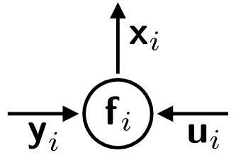
(a) Component uncertainty propagation

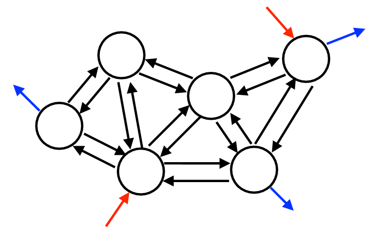
(b) Network uncertainty propagation

Figure 1: NetUQ formulation. Figure shows how the network uncertainty-propagation problem can be derived from component uncertainty-propagation problems shown in Fig. 1(a). In Fig. 1(b), black edges correspond to endogenous-input random variables ${\boldsymbol{\mathsf{y}}}$, red edges correspond to exogenous-input random variables ${\boldsymbol{\mathsf{u}}}$, and blue edges correspond to QoI random variables ${\boldsymbol{\mathsf{z}}}$. Note that output random variables ${\boldsymbol{\mathsf{x}}}$ are mapped to endogenous-input random variables ${\boldsymbol{\mathsf{y}}}$ and/or ${\boldsymbol{\mathsf{z}}}$ via the operators $\boldsymbol{\mathsf{I}}_{{\boldsymbol{\mathsf{x}}}}^{{\boldsymbol{\mathsf{y}}}}$ (see Eq. (7)) and $\boldsymbol{\mathsf{I}}_{{\boldsymbol{\mathsf{x}}}}^{{\boldsymbol{\mathsf{z}}}}$ (see Eq. (11)), respectively. We note that a network is defined from component uncertainty-propagation operators ${{\boldsymbol{\mathsf{f}}}}_{i}$, $i=1,\ldots,n$, the adjacency matrix $\boldsymbol{\mathsf{I}}_{{\boldsymbol{\mathsf{x}}}}^{{\boldsymbol{\mathsf{y}}}}$, and the extraction matrix $\boldsymbol{\mathsf{I}}_{{\boldsymbol{\mathsf{x}}}}^{{\boldsymbol{\mathsf{z}}}}$.

Remark 2.2 (Component independence).

This formulation promotes component independence, as the only formal inter-component compatibility requirement is the existence of an adjacency matrix $\boldsymbol{\mathsf{I}}_{{\boldsymbol{\mathsf{x}}}}^{{\boldsymbol{\mathsf{y}}}}$ that associates component output random variables with endogenous input random variables of other components. In particular, each set of random variables can be represented using different functional representations and components can employ completely different uncertainty-propagation operators.

3 Relaxation methods

In principle, the fixed-point system (8) can be solved using a variety of techniques. While Newton’s method is often employed for the solution of systems of nonlinear algebraic equations due to its local quadratic convergence rate, it relies on the ability to compute the gradient $\partial{\boldsymbol{\mathsf{r}}}/\partial{{\boldsymbol{\mathsf{x}}}}$. In the present context, this requires computing the gradient of the output random variables with respect to the endogenous-input random variables for each component, i.e., $\partial{{\boldsymbol{\mathsf{f}}}}_{i}/\partial{{\boldsymbol{\mathsf{y}}}}_{i}$ must be computable for $i=1,\ldots,n$. This is frequently impractical, e.g., when the simulation code used to compute a component uncertainty-propagation operator is available only as a “black box”.

As such, we proceed by assuming that only the component uncertainty-propagation operators ${{\boldsymbol{\mathsf{f}}}}_{i}$, $i=1,\ldots,n$ themselves are available, and consider classical relaxation methods (i.e., Jacobi, Gauss–Seidel) to solve the fixed-point problem (8), as these methods do not require gradients and promote component independence. If each node in the network corresponds to subdomain in a partial-differential-equation problem, then this approach can be considered an overlapping domain-decomposition strategy; however, the formulation does not rely on any particular interpretation of the components.

3.1 Jacobi method

We first consider applying a variant of the Jacobi method (i.e., additive Schwarz) to solve fixed-point problem (8); Algorithm 1 reports the algorithm. At each iteration, this approach performs independent, embarrassingly parallel component uncertainty propagation (Steps 3–5), applies a relaxation update (Step 6), and subsequently updates the endogenous-input random variables from the output random variables just computed for neighboring components (Step 7). From the network perspective, this approach is equivalent to “splitting” all endogenous-input edges at each iteration and allowing components to perform independent uncertainty propagation; see Figure 2(a).

At the network level, Jacobi iteration $k$ can be expressed simply as

(12) $$\tilde{\boldsymbol{\mathsf{x}}}={\boldsymbol{\mathsf{f}}}({\boldsymbol{\mathsf{x}}}^{(k)},{\boldsymbol{\mathsf{u}}})$$

(13) $${\boldsymbol{\mathsf{x}}}^{(k+1)}=\omega\tilde{\boldsymbol{\mathsf{x}}}+(1-\omega){\boldsymbol{\mathsf{x}}}^{(k)},$$

where $\omega>0$ is a relaxation factor, which is set to $\omega=1$ for the classical Jacobi method. Under-relaxation corresponds to $\omega<0$, while over-relaxation corresponds to $\omega>1$. This parameter controls convergence of the algorithm as well as error analysis as will be discussed in Remarks LABEL:rem:controlConverge and LABEL:rem:satisfyAss.

(a) Jacobi method

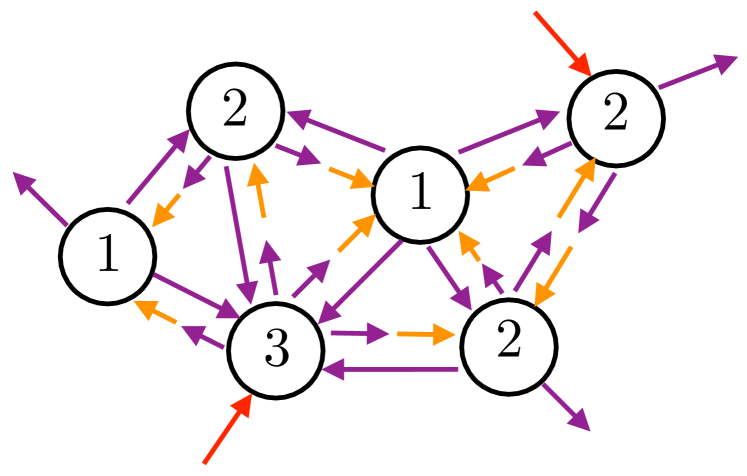
(b) Gauss–Seidel method

Figure 2: Relaxation methods. Here, random variables that were computed at the previous iteration are shown in orange, random variables that are computed at the current iteration are shown in violet, and exogenous-input random variables—whose values are fixed—are shown in red. For the Gauss–Seidel method, the order in which a given node is processed is included in Figure 2(b). For the Jacobi method, note that all edges associated with endogenous-input random variables are “split” at each iteration to enable embarrassingly parallel component uncertainty propagation. On the other hand, for the Gauss–Seidel method, only a subset of such edges are “split” at each iteration such that a directed acyclic graph (DAG) is created. As a result, each iteration corresponds to uncertainty propagation in a feed-forward network. In this example, the chosen edge splitting yields a DAG that incurs three sequential steps per iteration. Note that many such DAGs exist, and each associates with a particular permutation of the adjacency matrix $\boldsymbol{\mathsf{I}}_{{\boldsymbol{\mathsf{x}}}}^{{\boldsymbol{\mathsf{y}}}}$.

Algorithm 1 Jacobi (The Jacobi method for NetUQ)

Input: Component uncertainty-propagation operators ${{\boldsymbol{\mathsf{f}}}}_{i}$, $i=1,\ldots,n$; adjacency matrix $\boldsymbol{\mathsf{I}}_{{\boldsymbol{\mathsf{x}}}}^{{\boldsymbol{\mathsf{y}}}}$; exogenous-input random variables ${{\boldsymbol{\mathsf{u}}}}_{i}$, $i=1,\ldots,n$; initial guesses for endogenous-input random variables ${{\boldsymbol{\mathsf{y}}}}_{i}^{(0)}$, $i=1,\ldots,n$; relaxation factor $\omega$
Output: converged endogenous-input random variables ${{\boldsymbol{\mathsf{y}}}}_{i}^{(K)}$; converged output random variables ${{\boldsymbol{\mathsf{x}}}}_{i}^{(K)}$

1:  $k\leftarrow 0$

2:  while not converged do

3:     for $i=1,\ldots,n$ do {Execute in parallel}

4:        ${\tilde{\boldsymbol{\mathsf{x}}}}_{i}={{\boldsymbol{\mathsf{f}}}}_{i}({{\boldsymbol{\mathsf{y}}}}_{i}^{(k)},{{\boldsymbol{\mathsf{u}}}}_{i})$

5:     end for

6:      ${\boldsymbol{\mathsf{x}}}^{(k+1)}=\omega\tilde{\boldsymbol{\mathsf{x}}}+(1-\omega){\boldsymbol{\mathsf{x}}}^{(k)}$

7:      ${\boldsymbol{\mathsf{y}}}^{(k+1)}=\boldsymbol{\mathsf{I}}_{{\boldsymbol{\mathsf{x}}}}^{{\boldsymbol{\mathsf{y}}}}{\boldsymbol{\mathsf{x}}}^{(k+1)}$

8:     $k\leftarrow k+1$

9:  end while

10:  $K\leftarrow k$

3.2 Gauss–Seidel method

Naturally, we also consider a variant of the Gauss–Seidel method (i.e., multiplicative Schwarz) to solve fixed-point problem (8); Algorithm 2 reports the algorithm. The benefit of the Gauss–Seidel method with respect to the Jacobi method is that it enables more updated information to be used within each iteration, at the expense of reduced parallelism. To achieve this, each Gauss–Seidel iteration performs feed-forward uncertainty propagation, which requires “splitting” network edges in a manner that generates a directed acyclic graph (DAG), and subsequently performing feed-forward uncertainty propagation within the DAG; see Figure 2(b). In principle, each Gauss–Seidel iteration can employ a different DAG; for simplicity in exposition, we restrict consideration to a constant DAG.

Algorithm 2 GaussSeidel (The Gauss–Seidel method for NetUQ)

Input: Component uncertainty-propagation operators ${{\boldsymbol{\mathsf{f}}}}_{i}$, $i=1,\ldots,n$; adjacency matrix $\boldsymbol{\mathsf{I}}_{{\boldsymbol{\mathsf{x}}}}^{{\boldsymbol{\mathsf{y}}}}$; exogenous-input random variables ${{\boldsymbol{\mathsf{u}}}}_{i}$, $i=1,\ldots,n$; initial guesses for endogenous-input random variables ${{\boldsymbol{\mathsf{y}}}}_{i}^{(0)}$, $i=0,\ldots,n$; relaxation factor $\omega$; sequence of permutation matrices $\boldsymbol{p}^{(k)}$, $k=1,\ldots$
Output: converged endogenous-input random variables ${{\boldsymbol{\mathsf{y}}}}_{i}^{(K)}$; converged output random variables ${{\boldsymbol{\mathsf{x}}}}_{i}^{(K)}$

1:  $k\leftarrow 0$

2:  while not converged do

3:     $\boldsymbol{p}\leftarrow\boldsymbol{p}^{(k)}$

4:     $(\boldsymbol{\mathsf{P}}^{{\boldsymbol{\mathsf{x}}}}_{\boldsymbol{p}},\boldsymbol{\mathsf{P}}^{{\boldsymbol{\mathsf{y}}}}_{\boldsymbol{p}},\boldsymbol{\mathsf{L}}_{\boldsymbol{p}},\boldsymbol{\mathsf{U}}_{\boldsymbol{p}},\mathcal{I}_{\boldsymbol{p}},n_{\text{seq},\boldsymbol{p}})=\texttt{DAG}(\boldsymbol{p},\boldsymbol{\mathsf{I}}_{{\boldsymbol{\mathsf{x}}}}^{{\boldsymbol{\mathsf{y}}}})$

5:     $\bar{\boldsymbol{\mathsf{y}}}\leftarrow{\boldsymbol{\mathsf{y}}}^{(k)}$

6:     for $\ell=1,\ldots,n_{\text{seq},\boldsymbol{p}}$ do {Execute sequentially}

7:        for $i\in\mathcal{I}_{\boldsymbol{p}}^{\ell}$ do {Execute in parallel}

8:           ${\tilde{\boldsymbol{\mathsf{x}}}}_{i}={{\boldsymbol{\mathsf{f}}}}_{i}({\bar{\boldsymbol{\mathsf{y}}}}_{i},{{\boldsymbol{\mathsf{u}}}}_{i})$

9:           $\bar{\boldsymbol{\mathsf{y}}}\leftarrow\bar{\boldsymbol{\mathsf{y}}}+\boldsymbol{\mathsf{I}}_{{\boldsymbol{\mathsf{x}}}}^{{\boldsymbol{\mathsf{y}}}}[\boldsymbol{\mathsf{E}}^{{\boldsymbol{\mathsf{x}}}}_{i}]^{T}({\tilde{\boldsymbol{\mathsf{x}}}}_{i}-{{\boldsymbol{\mathsf{x}}}}_{i}^{(k)})$

10:        end for

11:     end for

12:      ${\boldsymbol{\mathsf{x}}}^{(k+1)}=\omega\tilde{\boldsymbol{\mathsf{x}}}+(1-\omega){\boldsymbol{\mathsf{x}}}^{(k)}$

13:      ${\boldsymbol{\mathsf{y}}}^{(k+1)}=\boldsymbol{\mathsf{I}}_{{\boldsymbol{\mathsf{x}}}}^{{\boldsymbol{\mathsf{y}}}}{\boldsymbol{\mathsf{x}}}^{(k+1)}$

14:     $k\leftarrow k+1$

15:  end while

16:  $K\leftarrow k$

To generate a DAG, we introduce $n$-tuple $\boldsymbol{p}\equiv(p_{1},\ldots,p_{n})\in\mathbb{N}^{n}$ that provides a permutation of natural numbers one to $n$. We then define the block permutation matrices

(14) $$\boldsymbol{\mathsf{P}}^{{\boldsymbol{\mathsf{x}}}}_{\boldsymbol{p}}\coloneqq\begin{bmatrix}\boldsymbol{\mathsf{E}}^{{\boldsymbol{\mathsf{x}}}}_{p_{1}}\\ \vdots\\ \boldsymbol{\mathsf{E}}^{{\boldsymbol{\mathsf{x}}}}_{p_{n}}\end{bmatrix},\quad\boldsymbol{\mathsf{P}}^{{\boldsymbol{\mathsf{y}}}}_{\boldsymbol{p}}\coloneqq\begin{bmatrix}\boldsymbol{\mathsf{E}}^{{\boldsymbol{\mathsf{y}}}}_{p_{1}}\\ \vdots\\ \boldsymbol{\mathsf{E}}^{{\boldsymbol{\mathsf{y}}}}_{p_{n}}\end{bmatrix}$$

and block decomposition of the permuted adjacency matrix

(15) $$\boldsymbol{\mathsf{P}}^{{\boldsymbol{\mathsf{y}}}}_{\boldsymbol{p}}\boldsymbol{\mathsf{I}}_{{\boldsymbol{\mathsf{x}}}}^{{\boldsymbol{\mathsf{y}}}}[\boldsymbol{\mathsf{P}}^{{\boldsymbol{\mathsf{x}}}}_{\boldsymbol{p}}]^{T}=\boldsymbol{\mathsf{L}}_{\boldsymbol{p}}+\boldsymbol{\mathsf{U}}_{\boldsymbol{p}},$$

where $\boldsymbol{\mathsf{L}}_{\boldsymbol{p}}\in\{0,1\}^{n_{\boldsymbol{\mathsf{y}}}\times n_{\boldsymbol{\mathsf{x}}}}$ is strictly block lower triangular and $\boldsymbol{\mathsf{U}}_{\boldsymbol{p}}\in\{0,1\}^{n_{\boldsymbol{\mathsf{y}}}\times n_{\boldsymbol{\mathsf{x}}}}$ is strictly block upper triangular.

By “splitting” all edges in the adjacency matrix $\boldsymbol{\mathsf{I}}_{{\boldsymbol{\mathsf{x}}}}^{{\boldsymbol{\mathsf{y}}}}$ whose indices match the nonzero elements of $[\boldsymbol{\mathsf{P}}^{{\boldsymbol{\mathsf{y}}}}_{\boldsymbol{p}}]^{T}\boldsymbol{\mathsf{U}}_{\boldsymbol{p}}\boldsymbol{\mathsf{P}}^{{\boldsymbol{\mathsf{x}}}}_{\boldsymbol{p}}$, we can create a DAG, as the components can be processed in sequential order $p_{i}$, $i=1,\ldots,n$. At the network level, Gauss–Seidel iteration $k$ can be expressed as

(16) $$\tilde{\boldsymbol{\mathsf{x}}}={\boldsymbol{\mathsf{f}}_{\text{vec}}}([\boldsymbol{\mathsf{P}}^{{\boldsymbol{\mathsf{y}}}}_{\boldsymbol{p}}]^{T}\boldsymbol{\mathsf{L}}_{\boldsymbol{p}}\boldsymbol{\mathsf{P}}^{{\boldsymbol{\mathsf{x}}}}_{\boldsymbol{p}}\tilde{\boldsymbol{\mathsf{x}}}+[\boldsymbol{\mathsf{P}}^{{\boldsymbol{\mathsf{y}}}}_{\boldsymbol{p}}]^{T}\boldsymbol{\mathsf{U}}_{\boldsymbol{p}}\boldsymbol{\mathsf{P}}^{{\boldsymbol{\mathsf{x}}}}_{\boldsymbol{p}}{\boldsymbol{\mathsf{x}}}^{(k)},{\boldsymbol{\mathsf{u}}})$$

(17) $${\boldsymbol{\mathsf{x}}}^{(k+1)}=\omega\tilde{\boldsymbol{\mathsf{x}}}+(1-\omega){\boldsymbol{\mathsf{x}}}^{(k)},$$

where again $\omega>0$ is a relaxation factor and the implicit expression (16) can be rewritten explicitly via recursion as

(18) $${\tilde{\boldsymbol{\mathsf{x}}}}_{p_{i}}={{\boldsymbol{\mathsf{f}}}}_{p_{i}}\left(\boldsymbol{\mathsf{E}}^{{\boldsymbol{\mathsf{y}}}}_{p_{i}}\boldsymbol{\mathsf{I}}_{{\boldsymbol{\mathsf{x}}}}^{{\boldsymbol{\mathsf{y}}}}\sum_{j=1}^{i-1}[\boldsymbol{\mathsf{E}}^{{\boldsymbol{\mathsf{x}}}}_{p_{j}}]^{T}{\tilde{\boldsymbol{\mathsf{x}}}}_{p_{j}}+\boldsymbol{\mathsf{E}}^{{\boldsymbol{\mathsf{y}}}}_{p_{i}}\boldsymbol{\mathsf{I}}_{{\boldsymbol{\mathsf{x}}}}^{{\boldsymbol{\mathsf{y}}}}\sum_{j=i+1}^{n}[\boldsymbol{\mathsf{E}}^{{\boldsymbol{\mathsf{x}}}}_{p_{j}}]^{T}\boldsymbol{\mathsf{E}}^{{\boldsymbol{\mathsf{x}}}}_{p_{j}}{\boldsymbol{\mathsf{x}}}^{(k)},{\boldsymbol{\mathsf{u}}}\right),\quad i=1,\ldots,n.$$

By comparing with the Jacobi update (12), it is apparent that the Gauss–Seidel update to $\tilde{\boldsymbol{\mathsf{x}}}$ in Eq. (16) is implicit rather than explicit, and so uses more updated information than Jacobi at each iteration; however, this is done at the expense of requiring sequential processing of the components.

To mitigate the sequential-processing burden, we observe that additional parallelism may be exposed by examining the sparsity pattern of $\boldsymbol{\mathsf{L}}_{\boldsymbol{p}}$, as this matrix encodes dependencies among the preserved edges in the (permuted) network.

Algorithm 3 describes this process. Given a permutation tuple $\boldsymbol{p}$, this algorithm effectively “splits” all edges associated with nonzero elements of $[\boldsymbol{\mathsf{P}}^{{\boldsymbol{\mathsf{y}}}}_{\boldsymbol{p}}]^{T}\boldsymbol{\mathsf{U}}_{\boldsymbol{p}}\boldsymbol{\mathsf{P}}^{{\boldsymbol{\mathsf{x}}}}_{\boldsymbol{p}}$, and analyzes the sparsity pattern of the block lower triangular matrix $\boldsymbol{\mathsf{L}}_{\boldsymbol{p}}$ to determine (1) the minimum number of sequential steps required to propagate uncertainties in the resulting DAG, and (2) which components can be processed within each sequential step. This procedure is called in Step 4 of Algorithm 2 to ensure the Gauss–Seidel iterations employ the fewest number of sequential steps. Clearly, different permutations $\boldsymbol{p}$ will associate with different numbers of required sequential steps; graph coloring [jensen2011graph] provides a mechanism to determine the minimum number of sequential steps for a given network. In addition to this consideration, different permutations may lead to different convergence rates as will be discussed in Remark LABEL:rem:controlConverge.

Algorithm 3 DAG (Generate a DAG from a permutation)

Input: Permutation $\boldsymbol{p}\equiv(p_{1},\ldots,p_{n})$ of the natural numbers one to $n$; adjacency matrix $\boldsymbol{\mathsf{I}}_{{\boldsymbol{\mathsf{x}}}}^{{\boldsymbol{\mathsf{y}}}}$
Output: Permutation matrices $\boldsymbol{\mathsf{P}}^{{\boldsymbol{\mathsf{x}}}}_{\boldsymbol{p}}$ and $\boldsymbol{\mathsf{P}}^{{\boldsymbol{\mathsf{y}}}}_{\boldsymbol{p}}$; block lower and upper triangular matrices $\boldsymbol{\mathsf{L}}_{\boldsymbol{p}}$ and $\boldsymbol{\mathsf{U}}_{\boldsymbol{p}}$; tuple of components in sequential processing order $\mathcal{I}_{\boldsymbol{p}}\coloneqq(\mathcal{I}_{\boldsymbol{p}}^{1},\ldots,\mathcal{I}_{\boldsymbol{p}}^{n_{\text{seq},\boldsymbol{p}}})$; number of sequential steps $n_{\text{seq},\boldsymbol{p}}$

1:  Compute $\boldsymbol{\mathsf{P}}^{{\boldsymbol{\mathsf{x}}}}_{\boldsymbol{p}}$, $\boldsymbol{\mathsf{P}}^{{\boldsymbol{\mathsf{y}}}}_{\boldsymbol{p}}$, $\boldsymbol{\mathsf{L}}_{\boldsymbol{p}}$, and $\boldsymbol{\mathsf{U}}_{\boldsymbol{p}}$ from Eqs. (14) and (15).

2:  $k\leftarrow 0$; $\mathcal{I}=\emptyset$

3:  while $\mathcal{I}\neq\{1,\ldots,n\}$ do

4:     $k\leftarrow k+1$

5:     $\mathcal{I}_{\boldsymbol{p}}^{k}\leftarrow\emptyset$

6:     for $i=1,\ldots,n$ do

7:        if block $(i,j)$ of $\boldsymbol{\mathsf{L}}_{\boldsymbol{p}}$ is zero for all $j\in\{1,\ldots,n\}\setminus\mathcal{I}$ then

8:           $\mathcal{I}_{\boldsymbol{p}}^{k}\leftarrow\mathcal{I}_{\boldsymbol{p}}^{k}\cup p_{i}$

9:        end if

10:     end for

11:     $\mathcal{I}\leftarrow\mathcal{I}\cup\mathcal{I}_{\boldsymbol{p}}^{k}$

12:  end while

13:  $n_{\text{seq},\boldsymbol{p}}=k$