Multi-Level Composite Stochastic Optimization via Nested Variance Reduction

Abstract

We consider multi-level composite optimization problems where each mapping in the composition is the expectation over a family of randomly chosen smooth mappings or the sum of some finite number of smooth mappings. We present a normalized proximal approximate gradient (NPAG) method where the approximate gradients are obtained via nested variance reduction. In order to find an approximate stationary point where the expected norm of its gradient mapping is less than $\epsilon$, the total sample complexity of our method is $O(\epsilon^{-3})$ in the expectation case, and $O(N+\sqrt{N}\epsilon^{-2})$ in the finite-sum case where $N$ is the total number of functions across all composition levels. In addition, the dependence of our total sample complexity on the number of composition levels is polynomial, rather than exponential as in previous work.

keywords:

composite stochastic optimization, proximal gradient method, variance reduction

1 Introduction

In this paper, we consider multi-level composite stochastic optimization problems of the form

$$\mathop{\textrm{minimize}}_{x\in\mathbf{R}^{d}}\quad\mathbf{E}_{\xi_{m}}\bigl{[}f_{m,\xi_{m}}\bigl{(}\cdots\mathbf{E}_{\xi_{2}}\bigl{[}f_{2,\xi_{2}}\bigl{(}\mathbf{E}_{\xi_{1}}\!\left[f_{1,\xi_{1}}(x)\right]\bigr{)}\bigr{]}\cdots\bigr{)}\bigr{]}+\Psi(x),$$ (1)

where $\xi_{1},\ldots,\xi_{m}$ are independent random variables. We assume that each realization of $f_{i,\xi_{i}}:\mathbf{R}^{d_{i-1}}\to\mathbf{R}^{d_{i}}$ is a smooth vector mapping (with $d_{0}=d$ and $d_{m}=1$) and the function $\Psi$ is convex but possibly nonsmooth. An interesting special case is when each $\xi_{i}$ follows the uniform distribution over a finite support $\{1,\ldots,N_{i}\}$, i.e.,

$$\mathop{\textrm{minimize}}_{x\in\mathbf{R}^{d}}\quad\frac{1}{N_{m}}\sum_{j=1}^{N_{m}}f_{m,j}\biggl{(}\cdots\frac{1}{N_{2}}\sum_{j=1}^{N_{2}}f_{2,j}\biggl{(}\frac{1}{N_{1}}\sum_{j=1}^{N_{1}}f_{1,j}(x)\biggr{)}\cdots\biggr{)}+\Psi(x).$$ (2)

To simplify presentation, we write the above problems as

$$\mathop{\textrm{minimize}}_{x\in\mathbf{R}^{d}}~{}\bigl{\{}\Phi(x)\triangleq F(x)+\Psi(x)\bigr{\}},$$ (3)

where the smooth part of the objective possesses a multi-level compositional structure:

$$F(x)=f_{m}\circ f_{m-1}\circ\cdots\circ f_{1}(x).$$ (4)

For problems (1) we use the definition $f_{i}(\cdot)=\mathbf{E}_{\xi_{i}}[f_{i,\xi_{i}}(\cdot)]$ and for problem (2), we have $f_{i}(\cdot)=(1/N_{i})\sum_{j=1}^{N_{i}}f_{i,j}(\cdot)$.

The formulations (1) and (2) cover a broader range of applications beyond the classical stochastic programming and empirical risk minimization (ERM) problems, which are special cases of (1) and (2) when $m=1$, respectively. Important applications with $m=2$ include policy evaluation in reinforcement learning and Markov decision processes (e.g., [34, 7]), risk-averse optimization (e.g., [31, 33]), and stochastic variational inequality (e.g., [17, 19] through a novel formulation in [15]). Other applications in machine learning and statistics include optimization of conditional random fields (CRF), Cox’s partial likelihood and expectation-maximization; see formulations in [6, Section 3.1-3.3]. Multi-level composite risk minimization problems with $m>2$ have been considered in, e.g.,  [10] and [39]. A more recent application of the multi-level problem is adversarial attacks and defenses in deep neural networks; see the survey paper [40].

1.1 Related work

Existing work on composite stochastic optimization traces back to [12]. Several recent progresses have been made for two-level ($m=2$) problems, both for the general stochastic formulation (e.g., [35, 36, 39, 15]) and for the finite-sum formulation (e.g., [20, 43, 16, 41]).

In order to cite specific results, we first explain the measure of efficiency for composite stochastic optimization. A well-adopted measure is their sample complexity, i.e., the total number of times that any component mapping $f_{i,\xi_{i}}(\cdot)$ or Jacobian $f^{\prime}_{i,\xi_{i}}(\cdot)$ is evaluated, in order to find some $\bar{x}$ (output of a randomized algorithm) such that $\mathbf{E}[\|\mathcal{G}(\bar{x})\|^{2}]\leq\varepsilon$ for a given precision $\varepsilon>0$. Here $\mathcal{G}(\bar{x})$ is the proximal gradient mapping of the objective function $\Phi\equiv F+\Psi$ at $\bar{x}$ (exact definition given in Section 2). If $\Psi\equiv 0$, then $\mathcal{G}(\bar{x})=F^{\prime}(\bar{x})$ where $F^{\prime}$ denotes the gradient of $F$ and the criteria for $\varepsilon$-approximation becomes $\mathbf{E}[\|F^{\prime}(\bar{x})\|^{2}]\leq\varepsilon$.

For problem (1) with two levels ($m=2$) and $\Psi\equiv 0$, stochastic composite gradient methods were developed in [35] with sample complexities $O(\varepsilon^{-4})$, $O(\varepsilon^{-3.5})$ and $O(\varepsilon^{-1.25})$ for the smooth nonconvex case, smooth convex case and smooth strongly convex case respectively. For nontrivial convex $\Psi$, improved sample complexities of $O(\varepsilon^{-2.25})$, $O(\varepsilon^{-2})$ and $O(\varepsilon^{-1})$ were obtained in [36] for the three cases respectively. These algorithms employ two-level stochastic updates in different time scales, i.e., the two step-size sequences converge to zero at different rates. Similar algorithms for solving multi-level problems were proposed in [39], with sample complexity $O(\varepsilon^{-(m+7)/4})$. A single time-scale method is proposed in [15] for solving two-level problems, which achieves an $O(\varepsilon^{-2})$ sample complexity, matching the result for single-level stochastic optimization [14].

For the composite finite-sum problem (2) with two levels ($m=2$), several recent works applied stochastic variance-reduction techniques to obtain improved sample complexity. Stochastic variance-reduction techniques were first developed for one-level finite-sum convex optimization problems (e.g., [32, 18, 8, 38, 4, 24]), and later extended to the one-level nonconvex setting (e.g., [27, 29, 3, 1, 2, 13, 37, 25, 26]) and the two-level finite-sum nonconvex setting (e.g., [20, 43, 16, 41]). For the two-level finite-sum case, the previous best known sample complexity is $O(N+N^{2/3}\varepsilon^{-1})$ where $N=N_{1}+N_{2}$, obtained in [16, 41].

Interestingly, better complexity bounds have been obtained recently for the non-composite case of $m=1$, specifically, $O(\varepsilon^{-1.5})$ for the expectation case and $O(N_{1}+\sqrt{N_{1}}\varepsilon^{-1})$ for the finite-sum case [13, 37, 25, 26]. These results look to be even better than the classical $O(\varepsilon^{-2})$ complexity of stochastic gradient method for single-level smooth nonconvex optimization (e.g., [14]), which is consistent with the statistical lower bound for sample average approximation [10]. Indeed, a stronger smoothness assumption is responsible for the improvement: instead of the classical assumption that the gradient of the expected function is Lipschitz continuous, the improved results require a Mean-Square-Lipschitz (MSL) condition (exact definition given in Section 3).

Different from the one-level case, a major difficulty in the multi-level cases ($m\geq 2$) is to deal with biased gradient estimators for the composite function (e.g., [35, 36, 41]). Unbiased gradient estimators for two-level problems are developed in [6], but they do not seem to improve sample complexity. On the other hand, it is shown in [42] that the improved sample complexity of $O\bigl{(}\min\{\varepsilon^{-1.5},\sqrt{N_{1}}\varepsilon^{-1}\}\bigr{)}$ can be obtained with biased gradient estimator for two-level problems where the outer level is deterministic or without finite-sum. This result indicates that similar improvements are possible for multi-level problems as well.

1.2 Contributions and outline

In this paper, we propose stochastic gradient algorithms with nested variance-reduction for solving problems (1) and (2) for any $m\geq 1$, and show that their sample complexity for finding $\bar{x}$ such that $\mathbf{E}[\|\mathcal{G}(\bar{x})\|]\leq\epsilon$ is $O(\epsilon^{-3})$ for the expectation case, and $O(N+\sqrt{N}\epsilon^{-2})$ for the finite-sum case where $N=\sum_{i=1}^{m}N_{i}$. To compare with previous work listed in Section 1.1, we note that a complexity $O(\varepsilon^{-a})$ for $\mathbf{E}[\|\mathcal{G}(\bar{x})\|^{2}]\leq\varepsilon$ (measure used in Section 1.1) implies an $O(\epsilon^{-2a})$ complexity for $\mathbf{E}[\|\mathcal{G}(\bar{x})\|]\leq\epsilon$ (by Jensen’s inequality, but not vice versa); in other words, $\varepsilon=O(\epsilon^{2})$. In this sense, our results are of the same orders as the best known sample complexities for solving one-level stochastic optimization problems [13, 37, 25, 26], and they are strictly better than previous results for solving two and multi-level problems.

The improvement in our results relies on a nested variance-reduction scheme using mini-batches and a stronger uniform Lipschitz assumption. Specifically, we assume that each realization of the random mapping $f_{i,\xi_{i}}$ and its Jacobian are Lipschitz continuous. This condition is stronger than the MSL condition assumed in [13, 37, 25, 26] for obtaining the $O\bigl{(}\min\{\epsilon^{-3},\sqrt{N_{1}}\epsilon^{-2}\}\bigr{)}$ sample complexity for one-level problems. Nevertheless, it holds for many applications in machine learning (e.g., [7, 6, 41]), especially when $\mathrm{dom\,}\Psi$ is bounded. The results in [39] also rely on such a uniform smooth condition.

Our contributions can be summarized as follows. In Section 2, we consider solving more general problems of the form (3) without specifying any composition structure, and propose a Normalized Proximal Approximate Gradient (NPAG) method. We show that so long as the Mean Square Errors (MSEs) of the approximate gradients at each iteration are uniformly bounded by $\epsilon^{2}$, then the iteration complexity of NPAG for finding an $\bar{x}$ such that $\mathbf{E}\|\mathcal{G}(\bar{x})\|]\leq\epsilon$ is $O(\epsilon^{-2})$.

In Section 3, we discuss stochastic variance-reduction techniques for constructing the approximate gradients in NPAG. In particular, we present a simple and unified perspective on variance reduction under the MSL condition. This perspective clearly explains the reason for periodic restart, and allows us to derive the optimal period length and mini-batch sizes without binding to any particular optimization algorithm. When using the SARAH/Spider estimator ([24] and [13] respectively) in NPAG to solve one-level stochastic or finite-sum problems, we obtain a Prox-Spider method. We also analyze the SVRG [18] and SAGA [8] estimators in the same framework, and obtain the best-known complexities for them in the literature for nonconvex optimization.

In Section 4, we present the multi-level Nested-Spider method and show that under the uniform Lipschitz condition (stronger than MSL), its sample complexity for the expectation is $O(m^{4}\epsilon^{-3})$ and for the finite-sum cases is $O(N+m^{4}\sqrt{N}\epsilon^{-1})$ where $N=\sum_{i=1}^{m}N_{i}$. In particular, these results are polynomial in the number of levels $m$, which improve significantly over the previous result $O(\epsilon^{-(m+7)/2})$ in [39], where $m$ appears in the exponent of $\epsilon$.

In Section 5, we present numerical experiments to compare different variance reduction methods on two applications, with one-level and two-level composition structure respectively. Finally, we give some concluding remarks in Section 6.

2 Normalized proximal approximate gradient method

In this section, we present a normalized proximal approximate gradient (NPAG) method for solving problems of form (3), which we repeat here for convenience:

$$\mathop{\textrm{minimize}}_{x\in\mathbf{R}^{d}}~{}\left\{\Phi(x)\triangleq F(x)+\Psi(x)\right\}.$$ (5)

Here we consider a much more general setting, without imposing any compositional structure on $F$. Formally, we have the following assumption.

Assumption 2.1.

The functions $F$, $\Psi$ and $\Phi$ in (5) satisfy:

• $F:\mathbf{R}^{d}\to\mathbf{R}$ is differentiable and its gradient $F^{\prime}$ is $L$-Lipschitz continuous;

• $\Psi:\mathbf{R}^{d}\to\mathbf{R}\cup\{+\infty\}$ is convex and lower semi-continuous;

• $\Phi\equiv F+\Psi$ is bounded below, i.e., there exists $\Phi_{*}$ such that $\Phi(x)\geq\Phi_{*}$ for all $x\in\mathrm{dom\,}\Psi$.

Under Assumption 2.1, we define the proximal operater of $\Psi$, with step size $\eta$, as

$$\mathbf{prox}_{\Psi}^{\eta}(x)\triangleq\mathop{\rm arg\,min}_{y\in\mathbf{R}^{d}}\left\{\Psi(y)+\frac{1}{2\eta}\|y-x\|^{2}\right\},\qquad x\in\mathrm{dom\,}\Psi.$$ (6)

Since $\Psi$ is convex, this operator is well defined and unique for any $x\in\mathrm{dom\,}\Psi$. Given the gradient of $F$ at $x$, denoted as $F^{\prime}(x)$, the proximal gradient mapping of $\Phi$ at $x$ is defined as

$$\mathcal{G}_{\Phi}^{\eta}(x)\triangleq\frac{1}{\eta}\Bigl{(}x-\mathbf{prox}_{\Psi}^{\eta}\bigl{(}x-\eta F^{\prime}(x)\bigr{)}\Bigr{)}.$$ (7)

When $\Psi\equiv 0$, we have $\mathcal{G}_{\Phi}^{\eta}(x)=F^{\prime}(x)$ for any $\eta>0$. Additional properties of the proximal gradient mapping are given in [22]. Throughout this paper, we denote the proximal gradient mapping as $\mathcal{G}(\cdot)$ by omitting the subscript $\Phi$ and superscript $\eta$ whenever they are clear from the context.

Our goal is to find an $\epsilon$-stationary point $\bar{x}$ such that $\|\mathcal{G}(\bar{x})\|\leq\epsilon$, or $\mathbf{E}\bigl{[}\|\mathcal{G}(\bar{x})\|\bigr{]}\leq\epsilon$ if using a stochastic or randomized algorithm (see [11] for justifications of $\|\mathcal{G}(\cdot)\|$ as a termination criterion). If the full gradient oracle $F^{\prime}(\cdot)$ is available, we can use the proximal gradient method

$$x^{t+1}=\mathbf{prox}_{\Psi}^{\eta}\bigl{(}x^{t}-\eta F^{\prime}(x^{t})\bigr{)}.$$ (8)

By setting $\eta=1/L$ where $L$ is the Lipschitz constant of $F^{\prime}$, this algorithm finds an $\epsilon$-stationary point within $O(L\epsilon^{-2})$ iterations; see, e.g., [5, Theorem 10.15].

Here we focus on the case where the full gradient oracle $F^{\prime}(\cdot)$ is not available; instead, we can compute at each iteration $t$ an approximate gradient $v^{t}$. A straightforward approach is to replace $F^{\prime}(x^{t})$ with $v^{t}$ in (8), and then analyze its convergence properties based on certain measures of approximation quality such as $\mathbf{E}[\|v^{t}-F^{\prime}(x^{t})\|^{2}]$. In Algorithm 1, we present a more sophisticated variant, which first compute a tentative iterate $\tilde{x}^{t+1}=\mathbf{prox}_{\Psi}^{\eta}(x^{t}-\eta v^{t})$, and then move in the direction of $\tilde{x}^{t+1}-x^{t}$ with a step size $\gamma_{t}$, i.e., $x^{t+1}=x^{t}+\gamma_{t}(\tilde{x}^{t+1}-x^{t})$. The choice of step size $\gamma_{t}=\min\left\{\frac{\eta\epsilon_{t}}{\|\tilde{x}^{t+1}-x^{t}\|},1\right\}$ ensures that the step length $\|x^{t+1}-x^{t}\|$ is always bounded:

$$\|x^{t+1}-x^{t}\|=\gamma_{t}\|\tilde{x}^{t+1}-x^{t}\|\leq\eta\epsilon_{t},$$ (9)

where $\epsilon_{t}$ is a pre-specified parameter.

input: initial point $x^{0}\in\mathbf{R}^{d}$, proximal step size $\eta>0$, a sequence $\epsilon_{t}>0,\forall t$.

for $t=0,...,T-1$ do

       Find an approximate gradient $v^{t}$ at the point $x^{t}$.

      [0.5ex] Compute $\tilde{x}^{t+1}=\mathbf{prox}_{\Psi}^{\eta}(x^{t}-\eta v^{t}).$

       Update $x^{t+1}=x^{t}+\gamma_{t}(\tilde{x}^{t+1}-x^{t})$ with $\gamma_{t}=\min\left\{\frac{\eta\,\epsilon_{t}}{\|\tilde{x}^{t+1}-x^{t}\|},~{}1\right\}$.

end for

output: $\!\bar{x}\!\in\!\{x^{0}\!,...,x^{T\!-\!1}\}$, with $x^{t}$ chosen w.p. $p_{t}:=\frac{\epsilon_{t}}{\sum_{k=0}^{T-1}\epsilon_{k}}$ for $0\leq t\leq T-1$.

Algorithm 1 Normalized Proximal Approximate Gradient (NPAG) Method

Algorithm 1 can also be written in terms of the approximate gradient mapping, which we define as

$$\widetilde{\mathcal{G}}(x^{t})=\frac{1}{\eta}\bigl{(}x^{t}-\tilde{x}^{t+1}\bigr{)}=\frac{1}{\eta}\bigl{(}x^{t}-\mathbf{prox}_{\Psi}^{\eta}(x^{t}-\eta v^{t})\bigr{)}.$$ (10)

Using this notation, the updates in Algorithm 1 become $\gamma_{t}=\min\Bigl{\{}\frac{\epsilon_{t}}{\left\|\widetilde{\mathcal{G}}(x^{t})\right\|},1\Bigr{\}}$ and

$$x^{t+1}=x^{t}-\gamma_{t}\eta\,\widetilde{\mathcal{G}}(x^{t})=\left\{\begin{array}[]{ll}x^{t}-\eta\epsilon_{t}\frac{\widetilde{\mathcal{G}}(x^{t})}{\left\|\widetilde{\mathcal{G}}(x^{t})\right\|}&\mbox{if}~{}\bigl{\|}\widetilde{\mathcal{G}}(x^{t})\bigr{\|}>\epsilon_{t},\\[6.45831pt] x^{t}-\eta\,\widetilde{\mathcal{G}}(x^{t})&\mbox{if}~{}\bigl{\|}\widetilde{\mathcal{G}}(x^{t})\bigr{\|}\leq\epsilon_{t}.\end{array}\right.$$

Notice that when $\bigl{\|}\widetilde{\mathcal{G}}(x^{t})\bigr{\|}>\epsilon_{t}$, the algorithm uses the normalized proximal gradient mapping with a step length $\eta\epsilon_{t}$. Therefore, we call it the Normalized Proximal Approximate Gradient (NPAG) method.

Next, we prove a general convergence result concerning Algorithm 1 without specifying how the approximate gradient $v^{t}$ is generated. The only condition we impose is that the Mean-Square Error (MSE), $\mathbf{E}[\|v^{t}-F^{\prime}(x^{t})\|^{2}]$, is sufficiently small for all $t$. We first state a useful lemma.

Lemma 2.2.

Suppose Assumption 2.1 hold. Then the sequence $\{x^{t}\}$ generated by Algorithm 1 satisfies

$$\Phi(x^{t+1})\leq\Phi(x^{t})-\left(\gamma_{t}/\eta-L\gamma_{t}^{2}\right)\bigl{\|}\tilde{x}^{t+1}-x^{t}\bigr{\|}^{2}+\frac{1}{2L}\bigl{\|}F^{\prime}(x^{t})-v^{t}\bigr{\|}^{2},\qquad\forall\,t\geq 0.$$

Proof.

According to the update rule for $x^{t+1}$, we have

$$\Phi(x^{t+1}) = F(x^{t}+\gamma_{t}(\tilde{x}^{t+1}-x^{t}))+\Psi(x^{t}+\gamma_{t}(\tilde{x}^{t+1}-x^{t}))$$ (11)

$$\leq F(x^{t})\!+\!\gamma_{t}\left\langle F^{\prime}(x^{t}),\tilde{x}^{t+1}\!\!-\!x^{t}\right\rangle\!+\!\frac{L\gamma^{2}_{t}}{2}\|\tilde{x}^{t+1}\!\!-\!x^{t}\|^{2}\!+\!(1\!-\!\gamma_{t})\Psi(x^{t})\!+\!\gamma_{t}\Psi(\tilde{x}^{t+1})$$

$$= F(x^{t})+\Psi(x^{t})+\frac{L\gamma^{2}_{t}}{2}\|\tilde{x}^{t+1}-x^{t}\|^{2}+\gamma_{t}\left\langle F^{\prime}(x^{t})-v^{t},\tilde{x}^{t+1}-x^{t}\right\rangle$$

$$+\gamma_{t}\Bigl{(}\left\langle v^{t},\tilde{x}^{t+1}-x^{t}\right\rangle+\Psi(\tilde{x}^{t+1})-\Psi(x^{t})\Bigr{)},$$

where the inequality is due to the $L$-smoothness of $F$ (see, e.g., [23, Lemma 1.2.3]) and the convexity of $\Psi$. Since $\tilde{x}^{t+1}$ is the minimizer of a $\frac{1}{\eta}$-strongly convex function, i.e.,

$$\tilde{x}^{t+1}=\mathbf{prox}_{\Psi}^{\eta}\bigl{(}x^{t}-\eta v^{t}\bigr{)}=\mathop{\rm arg\,min}_{y\in\mathbf{R}^{d}}\Bigl{\{}\langle v^{t},y-x^{t}\rangle+\Psi(y)+\frac{1}{2\eta}\|y-x^{t}\|^{2}\Bigr{\}},$$

we have

$$\langle v^{t},\tilde{x}^{t+1}-x^{t}\rangle+\Psi(\tilde{x}^{t+1})+\frac{1}{2\eta}\|\tilde{x}^{t+1}-x^{t}\|^{2}\leq\Psi(x^{t})-\frac{1}{2\eta}\|\tilde{x}^{t+1}-x^{t}\|^{2},$$

which implies

$$\left\langle v^{t},\tilde{x}^{t+1}-x^{t}\right\rangle+\Psi(\tilde{x}^{t+1})-\Psi(x^{t})~{}\leq~{}-\frac{1}{\eta}\bigl{\|}\tilde{x}^{t+1}-x^{t}\bigr{\|}^{2}.$$

Applying the above inequality to the last term in (11) yields

$$\Phi(x^{t+1}) \leq \Phi(x^{t})-\Bigl{(}\frac{\gamma_{t}}{\eta}-\frac{L\gamma_{t}^{2}}{2}\Bigr{)}\|\tilde{x}^{t+1}-x^{t}\|^{2}+\gamma_{t}\langle F^{\prime}(x^{t})-v^{t},\tilde{x}^{t+1}-x^{t}\rangle$$

$$\leq \Phi(x^{t})-\Bigl{(}\frac{\gamma_{t}}{\eta}-\frac{L\gamma_{t}^{2}}{2}\Bigr{)}\|\tilde{x}^{t+1}-x^{t}\|^{2}+\frac{L\gamma_{t}^{2}}{2}\|\tilde{x}^{t+1}-x^{t}\|^{2}+\frac{1}{2L}\|F^{\prime}(x^{t})-v^{t}\|^{2}$$

$$= \Phi(x^{t})-\Bigl{(}\frac{\gamma_{t}}{\eta}-L\gamma_{t}^{2}\Bigr{)}\|\tilde{x}^{t+1}-x^{t}\|^{2}+\frac{1}{2L}\|F^{\prime}(x^{t})-v^{t}\|^{2},$$

where the second inequality is due to the Cauchy-Schwarz inequality. ∎

We note this result is similar to that of [26, Lemma 3], but we used a slightly looser bound for the inner product in the last step. This bound and our choice of $\gamma_{t}$ allow a simple convergence analysis of the NPAG method, which we present next.

Theorem 2.3.

Suppose Assumption 2.1 hold and we set $\eta=1/2L$ in Algorithm 1. If it holds that

$$\mathbf{E}\left[\|v^{t}-F^{\prime}(x^{t})\|^{2}\right]\leq\epsilon_{t}^{2},\qquad\forall\,t\geq 0,$$ (12)

for some sequence $\{\epsilon_{t}\}$, then the output $\bar{x}$ of Algorithm 1 satisfies

$$\mathbf{E}\bigl{[}\|\mathcal{G}(\bar{x})\|\bigr{]}\leq\frac{4L(\Phi(x^{0})-\Phi_{*})}{\sum_{t=0}^{T-1}\epsilon_{t}}+\frac{4\sum_{t=0}^{T-1}\epsilon^{2}_{t}}{\sum_{t=0}^{T-1}\epsilon_{t}}.$$ (13)

Proof.

Using Lemma 2.2, the assumption (12), and the choice $\eta=1/2L$, we obtain

$$\mathbf{E}\left[\Phi(x^{t+1})\right] \leq \mathbf{E}\left[\Phi(x^{t})\right]-\mathbf{E}\left[\left(\gamma_{t}/\eta-L\gamma_{t}^{2}\right)\bigl{\|}\tilde{x}^{t+1}-x^{t}\bigr{\|}^{2}\right]+\frac{\epsilon_{t}^{2}}{2L}$$ (14)

$$= \mathbf{E}\left[\Phi(x^{t})\right]-\frac{1}{4L}\mathbf{E}\left[\Bigl{(}2\gamma_{t}-\gamma_{t}^{2}\Bigr{)}\|\widetilde{\mathcal{G}}(x^{t})\|^{2}\right]+\frac{\epsilon_{t}^{2}}{2L}$$

$$\leq \mathbf{E}\left[\Phi(x^{t})\right]-\frac{1}{4L}\mathbf{E}\left[\gamma_{t}\|\widetilde{\mathcal{G}}(x^{t})\|^{2}\right]+\frac{\epsilon_{t}^{2}}{2L},$$

where the equality is due to (10) and the last inequality is due to $0\leq\gamma_{t}\leq 1$, which implies $2\gamma_{t}-\gamma_{t}^{2}\geq\gamma_{t}$. Note that $\gamma_{t}=\min\Bigl{\{}\frac{\epsilon_{t}}{\left\|\widetilde{\mathcal{G}}(x^{t})\right\|},1\Bigr{\}}$, therefore

$$\gamma_{t}\bigl{\|}\widetilde{\mathcal{G}}(x^{t})\bigr{\|}^{2}=\epsilon^{2}_{t}\cdot\min\left\{\bigl{\|}\widetilde{\mathcal{G}}(x^{t})\bigr{\|}\epsilon_{t}^{-1},\,\bigl{\|}\widetilde{\mathcal{G}}(x^{t})\bigr{\|}^{2}\epsilon_{t}^{-2}\right\}\geq\epsilon_{t}\bigl{\|}\widetilde{\mathcal{G}}(x^{t})\bigr{\|}-\frac{1}{4}\epsilon_{t}^{2},$$

where the inequality is due to the fact $\min\bigl{\{}|z|,z^{2}\bigr{\}}\geq|z|-\frac{1}{4}$ for all $z\in\mathbf{R}$ (here we take $z=\epsilon_{t}^{-1}\|\tilde{\mathcal{G}}(x^{t})\|$). Taking expectations and substituting the above inequality into (14) gives

$$\mathbf{E}\left[\Phi(x^{t+1})\right]~{}\leq~{}\mathbf{E}\left[\Phi(x^{t})\right]-\frac{\epsilon_{t}}{4L}\mathbf{E}\left[\bigl{\|}\widetilde{\mathcal{G}}(x^{t})\bigr{\|}\right]+\frac{9\epsilon_{t}^{2}}{16L}.$$ (15)

On the other hand, by (12) and Jessen’s inequality we obtain

$$\mathbf{E}\left[\|v^{t}-F^{\prime}(x^{t})\|\right]\leq\sqrt{\mathbf{E}\left[\|v^{t}-F^{\prime}(x^{t})\|^{2}\right]}\leq\epsilon_{t}.$$

Denote $\hat{x}^{t+1}=\mathbf{prox}_{r}^{\eta}(x^{t}-\eta F^{\prime}(x^{t}))$ and also note that $\tilde{x}^{t+1}=\mathbf{prox}_{r}^{\eta}(x^{t}-\eta v^{t})$. Since the proximal operator is nonexpansive (see, e.g., [30, Section 31]), we have

$$\mathbf{E}\left[\|\hat{x}^{t+1}-\tilde{x}^{t+1}\|\right]\leq\eta\mathbf{E}[\|v^{t}-F^{\prime}(x^{t})\|]\leq\eta\epsilon_{t},\qquad\forall\,t\geq 0.$$

Therefore,

$$\mathbf{E}\bigl{[}\|\mathcal{G}(x^{t})\|\bigr{]}=\frac{1}{\eta}\mathbf{E}\bigl{[}\|\hat{x}^{t+1}-x^{t}\|\bigr{]} \leq \frac{1}{\eta}\mathbf{E}\bigl{[}\|\tilde{x}^{t+1}-x^{t}\|\bigr{]}+\frac{1}{\eta}\mathbf{E}\bigl{[}\|\hat{x}^{t+1}-\tilde{x}^{t+1}\|\bigr{]}$$

$$\leq \mathbf{E}\left[\bigl{\|}\widetilde{\mathcal{G}}(x^{t})\bigr{\|}\right]+\epsilon_{t}.$$

Combining the above inequality with (15), we get

$$\frac{\epsilon_{t}}{4L}\mathbf{E}\left[\bigl{\|}\mathcal{G}(x^{t})\bigr{\|}\right]~{}\leq~{}\mathbf{E}\left[\Phi(x^{t})\right]-\mathbf{E}\left[\Phi(x^{t+1})\right]+\frac{\epsilon^{2}_{t}}{L}.$$ (16)

Adding the above inequality for $k=0,...,T-1$ and rearranging the terms, we obtain

$$\mathbf{E}\left[\bigl{\|}\mathcal{G}(\bar{x})\bigr{\|}\right]=\sum_{k=0}^{T-1}\frac{\epsilon_{k}}{\sum_{t=0}^{T-1}\epsilon_{t}}\cdot\mathbf{E}\left[\bigl{\|}\mathcal{G}(x^{t})\bigr{\|}\right]\leq\frac{4L(\Phi(x^{0})-\Phi_{*})}{\sum_{t=0}^{T-1}\epsilon_{t}}+\frac{4\sum_{t=0}^{T-1}\epsilon^{2}_{t}}{\sum_{t=0}^{T-1}\epsilon_{t}}.$$

This completes the proof. ∎

Remark 2.4.

In the simplest case, one can set $\epsilon_{t}\equiv\epsilon$ for all $t=0,1,...,T-1$ and

$$T\geq 4L\left(\Phi(x^{0})-\Phi_{*}\right)\epsilon^{-2}.$$

Then Theorem 2.3 directly implies

$$\mathbf{E}\left[\bigl{\|}\mathcal{G}(\bar{x})\bigr{\|}\right]\leq\frac{4L(\Phi(x^{0})-\Phi_{*})}{T\epsilon}+\frac{4T\epsilon^{2}}{T\epsilon}\leq 5\epsilon.$$

Theorem 2.3 applies directly to the deterministic proximal gradient method with $v^{t}=F^{\prime}(x^{t})$. In this case, with $\epsilon_{t}$ and $T$ set according to Remark 2.4, condition (12) is automatically satisfied and we recover the $O(L\epsilon^{-2})$ complexity of proximal gradient method for nonconvex optimization [5, Theorem 10.15].

The problem of using a small, constant $\epsilon_{t}$ is that we will have very small step size $\gamma_{t}$ in the beginning iterations of the algorithm. Although the order of the sample complexity is optimal, it may lead to slow convergence in the practice. We will see in Section 4 that we can obtain the same orders of samples complexity using a variable sequence $\{\epsilon_{t}\}$, starting with large values and gradually decreases to the target precision $\epsilon$. These choices of variable sequence $\{\epsilon_{t}\}$ lead to improved performance in practice and are adopted in our numerical experiments in Section 5.

In general, for the stochastic problems, we do not require the estimates $v^{t}$ to be unbiased. On the other hand, condition (12) looks to be quite restrictive by requiring the MSE of approximate gradient to be less than $\epsilon_{t}^{2}$, where $\epsilon_{t}$ is some predetermined precision. In the rest of this paper, we show how to ensure condition (12) using stochastic variance-reduction techniques and derive the total sample complexity required for solving problems (1) and (2).

3 A general framework of stochastic variance reduction

In this section, we discuss stochastic variance-reduction techniques for smooth nonconvex optimization. In order to prepare for the multi-level compositional case, we proceed with a general framework of constructing stochastic estimators that satisfies (12) for Lipschitz-continuous vector or matrix mappings. To simplify presentation, we restrict our discussion in this section to the setting where $\epsilon_{t}\equiv\epsilon$ in (12), where $\epsilon$ is the target precsion so that the output $\bar{x}$ satisfies $\mathbf{E}[\|\mathcal{G}(\bar{x})\|]\leq O(\epsilon)$. A more general scheme with variable sequence $\{\epsilon_{t}\}$ is presented in Section 4.

Consider a family of mappings $\{\phi_{\xi}:\mathbf{R}^{d}\to\mathbf{R}^{p\times q}\}$ where the index $\xi$ is a random variable. We assume that they satisfy a uniform Lipschitz condition, i.e., there exists $L>0$ such that

$$\|\phi_{\xi}(x)-\phi_{\xi}(y)\|\leq L\|x-y\|,\qquad\forall\,x,y\in\mathbf{R}^{d},\qquad\forall\,\xi\in\Omega,$$ (17)

where $\|\cdot\|$ denotes the matrix Frobenius norm and $\Omega$ is the sample space of $\xi$. This uniform Lipschitz condition implies the Mean-Squared Lipschitz (MSL) property, i.e.,

$$\mathbf{E}_{\xi}\bigl{[}\|\phi_{\xi}(x)-\phi_{\xi}(y)\|^{2}\bigr{]}\leq L^{2}\|x-y\|^{2},\qquad\forall x,y\in\mathbf{R}^{d},$$ (18)

which is responsible for obtaining the $O\bigl{(}\min\{\varepsilon^{-3},\sqrt{N_{1}}\varepsilon^{-2}\}\bigr{)}$ sample complexity for one-level problems in [13, 37, 25, 26]. This property in turn implies that the average mapping, defined as

$$\bar{\phi}(x)\triangleq\mathbf{E}_{\xi}[\phi_{\xi}(x)],$$

is $L$-Lipschitz. In addition, we make the standard assumption that they have bounded variance everywhere, i.e.,

$$\mathbf{E}_{\xi}[\|\phi_{\xi}(x)-\bar{\phi}(x)\|^{2}]\leq\sigma^{2},\qquad\forall x\in\mathbf{R}^{d}.$$ (19)

In the context of solving structured optimization problems of form (5), we can restrict the above assumptions to hold within $\mathrm{dom\,}\Psi$ instead of $\mathbf{R}^{d}$.

Suppose a stochastic algorithm generates a sequence $\{x^{0},x^{1},\ldots,\}$ using some recursive rule

$$x^{t+1}=\psi_{t}(x^{t},v^{t}),$$

where $v^{t}$ is a stochastic estimate of $\bar{\phi}(x^{t})$. As an example, consider using Algorithm 1 to solve problem (5) where the smooth part $F(x)=\mathbf{E}_{\xi}[f_{\xi}(x)]$. In this case, we have $\phi_{\xi}(x)=f^{\prime}_{\xi}(x)$ and $\bar{\phi}(x)=F^{\prime}(x)$, and can use the simple estimator $v^{t}=f^{\prime}_{\xi_{t}}(x^{t})$ where $\xi_{t}$ is a realization of the random variable at time $t$. If $\epsilon\geq\sigma$, then assumption (19) directly implies (12) with $\epsilon_{t}\equiv\epsilon$; thus Theorem 2.3 and Remark 2.4 show that the sample complexity of Algorithm 1 for obtaining $\mathbf{E}[\|\mathcal{G}(\bar{x})\|]\leq\epsilon$ is $T=O(L\epsilon^{-2})$.

However, if the desired accuracy $\epsilon$ is smaller than the uncertainty level $\sigma$, then condition (12) is not satisfied and we cannot use Theorem 2.3 directly. A common remedy is to use mini-batches; i.e., at each iteration of the algorithm, we randomly pick a subset $\mathcal{B}_{t}$ of $\xi$ and set

$$v^{t}=\phi_{\mathcal{B}_{t}}(x^{t})\triangleq\frac{1}{|\mathcal{B}_{t}|}\sum_{\xi\in\mathcal{B}_{t}}\phi_{\xi}(x^{t}).$$ (20)

In this case, we have $\mathbf{E}[v^{t}]=\bar{\phi}(x^{t})$ and $\mathbf{E}[\|v^{t}-\bar{\phi}(x^{t})\|^{2}]=\sigma^{2}/|\mathcal{B}_{t}|$. In order to satisfy (12) with $\epsilon_{t}\equiv\epsilon$, we need $|\mathcal{B}_{t}|\geq\sigma^{2}/\epsilon^{2}$ for all $t=0,\ldots,T-1$. Then we can apply Theorem 2.3 and Remark 2.4 to derive its sample complexity for obtaining $\mathbf{E}[\|\mathcal{G}(\bar{x})\|]\leq\epsilon$, which amounts to $T\cdot\sigma^{2}/\epsilon^{2}=O(L\sigma^{2}\epsilon^{-4})$.

Throughout this paper, we assume that the target precision $\epsilon<\sigma$. In this case (and assuming $\Psi\equiv 0$), the total sample complexity $O(L\epsilon^{-2}+\sigma^{2}\epsilon^{-4})$ can be obtained without using mini-batches (see, e.g., [14]). Therefore, using mini-batches alone seems to be insufficient to improve sample complexity (although it can facilitate parallel computing; see, e.g., [9]). Notice that the simple mini-batch estimator (20) does not rely on any Lipschitz condition, so it can also be used with non-Lipschitz mappings such as subgradients of nonsmooth convex functions. Under the MSL condition (18), several variance-reduction techniques that can significantly reduce the sample complexity of stochastic optimization have been developed in the literature (e.g., [32, 18, 8, 38, 4, 24, 13].

In order to better illustrate how Lipschitz continuity can help with efficient variance reduction, we consider the amount of samples required in constructing a number of, say $\tau$, consecutive estimates $\{v^{0},\ldots,v^{\tau-1}\}$ that satisfy

$$\mathbf{E}\bigl{[}\bigl{\|}v^{t}-\bar{\phi}(x^{t})\bigr{\|}^{2}\bigr{]}\leq\epsilon^{2},\quad t=0,1,\ldots,\tau-1.$$ (21)

If the incremental step lengths $\|x^{t}-x^{t-1}\|$ for $t=1,\ldots,\tau-1$ are sufficiently small and the period $\tau$ is not too long, then one can leverage the MSL condition (18) to reduce the total sample complexity, to be much less than using the simple mini-batch estimator (20) for all $\tau$ steps. In the rest of this section, we first study the SARAH/Spider estimator proposed in [24] and [13] respectively. Then we also analyze the SVRG [18] and SAGA [8] estimators from the same general framework.

3.1 SARAH/SPIDER estimator for stochastic optimization

In order to construct $\tau$ consecutive estimates $\{v^{0},\ldots,v^{\tau-1}\}$, this estimator uses the mini-batch estimator (20) for $v^{0}$, and then constructs $v^{1}$ through $v^{\tau-1}$ using a recursion:

$$\begin{split}v^{0}&=\phi_{\mathcal{B}_{0}}(x^{0}),\\ v^{t}&=v^{t-1}+\phi_{\mathcal{B}_{t}}(x^{t})-\phi_{\mathcal{B}_{t}}(x^{t-1}).\end{split}$$ (22)

It was first proposed in [24] as a gradient estimator of SARAH (StochAstic Recursive grAdient algoritHm) for finite-sum convex optimization, and later extended to nonconvex and stochastic optimization [25, 26]. The form of (22) for general Lipschitz continuous mappings is proposed in [13], known as Spider (Stochastic Path-Integrated Differential EstimatoR). The following lemma is key to our analysis.

Lemma 3.1.

[13, Lemma 1] Suppose the random mappings $\phi_{\xi}$ satisfy (18). Then the MSE of the estimator in (22) can be bounded as

$$\mathbf{E}\left[\bigl{\|}v^{t}-\bar{\phi}(x^{t})\bigr{\|}^{2}\right]\leq\mathbf{E}\left[\bigl{\|}v^{0}-\bar{\phi}(x^{0})\bigr{\|}^{2}\right]+\sum_{r=1}^{t}\frac{L^{2}}{|\mathcal{B}_{r}|}\mathbf{E}\left[\|x^{r}-x^{r-1}\|^{2}\right].$$ (23)

If we can control the step lengths $\|x^{t}-x^{t-1}\|\leq\delta$ for $t=1,\ldots,\tau-1$, then

$$\mathbf{E}\left[\bigl{\|}v^{0}-\bar{\phi}(x^{0})\bigr{\|}^{2}\right]\leq\cdots\leq\mathbf{E}\left[\bigl{\|}v^{\tau-1}-\bar{\phi}(x^{\tau-1})\bigr{\|}^{2}\right]\leq\frac{\sigma^{2}}{|\mathcal{B}_{0}|}+\sum_{t=1}^{\tau-1}\frac{L^{2}\delta^{2}}{|\mathcal{B}_{t}|}.$$ (24)

To simplify notation, here we allow the batch sizes $|\mathcal{B}_{t}|$ to take fraction values, which does not change the order of required sample complexity. Now, in order to satisfy (21), it suffices to set

$$|\mathcal{B}_{0}|=\frac{2\sigma^{2}}{\epsilon^{2}}\quad\mbox{and}\quad|\mathcal{B}_{t}|=b=\frac{2\tau L^{2}\delta^{2}}{\epsilon^{2}},\quad t=1,\ldots,\tau-1.$$ (25)

In this case, the number of samples required over $\tau$ steps is

$$|\mathcal{B}_{0}|+(\tau-1)b~{}\leq~{}\frac{2\sigma^{2}}{\epsilon^{2}}+\frac{2\tau^{2}L^{2}\delta^{2}}{\epsilon^{2}}.$$

Therefore, it is possible to choose $\delta$ and $\tau$ to make the above number smaller than $\tau\sigma^{2}/\epsilon^{2}$, which is the number of samples required for (21) with the simple mini-batching scheme (20).

To make further simplifications, we choose $\delta=\epsilon/2L$, which leads to $b=\tau/2$ and

$$|\mathcal{B}_{0}|+(\tau-1)b~{}\leq~{}2\sigma^{2}/\epsilon^{2}+\tau^{2}/2.$$

The ratio between the numbers of samples required by Spider and simple mini-batching is

$$\rho(\tau)~{}\triangleq~{}\left(\frac{2\sigma^{2}}{\epsilon^{2}}+\frac{\tau^{2}}{2}\right)\bigg{/}\left(\tau\frac{\sigma^{2}}{\epsilon^{2}}\right)~{}=~{}\frac{2}{\tau}+\frac{\tau\epsilon^{2}}{2\sigma^{2}}.$$

In order to maximize the efficiency of variance reduction, we should choose $\tau$ to minimize this ratio, which is done by setting

$$\tau_{\star}=2\sigma/\epsilon.$$

Using (25) and $\delta=\epsilon/2L$, the corresponding mini-batch size and optimal ratio of saving are

$$b_{\star}=\tau_{\star}/2=\sigma/\epsilon,\qquad\rho(\tau_{\star})=2\,\epsilon/\sigma.$$ (26)

Therefore, significant reduction in sample complexity can be expected when $\epsilon\ll\sigma$.

input: initial point $x^{0}\in\mathbf{R}^{d}$, proximal step size $\eta>0$, and precision $\epsilon>0$;

           Spider epoch length $\tau$, large batch size $B$ and small batch size $b$.

for $t=0,1,...,T-1$ do

       if $t\bmod\tau==0$ then

             Randomly sample a batch $\mathcal{B}^{t}$ of $\xi$ with $|\mathcal{B}^{t}|=B$

             $v^{t}=f^{\prime}_{\mathcal{B}^{t}}(x^{t})$

      else

             Randomly sample a batch $\mathcal{B}^{t}$ of $\xi$ with $|\mathcal{B}^{t}|=b$

             $v^{t}=v^{t-1}+f^{\prime}_{\mathcal{B}^{t}}(x^{t})-f^{\prime}_{\mathcal{B}^{t}}(x^{t-1})$

       end if

      $\tilde{x}^{t+1}=\mathbf{prox}_{\Psi}^{\eta}(x^{t}-\eta v^{t})$

       $x^{t+1}=x^{t}+\gamma_{t}(\tilde{x}^{t+1}-x^{t})$ with $\gamma_{t}=\min\left\{\frac{\eta\,\epsilon}{\|\tilde{x}^{t+1}-x^{t}\|},~{}1\right\}$

end for

output: $\bar{x}$ uniformly sampled from $\{x^{0},...,x^{T-1}\}$.

Algorithm 2 Prox-Spider Method

The above derivation gives an optimal length $\tau_{\star}$ for variance reduction over consecutive estimates $\{v^{0},\ldots,v^{\tau-1}\}$. If the number of iterations required by the algorithm is lager than $\tau_{\star}$, then we need to restart the Spider estimator every $\tau_{\star}$ iterations. This way, we can keep the optimal ratio $\rho(\tau_{\star})$ to obtain the best total sample complexity.

Algorithm 2 is an instantiation of the NPAG method (Algorithm 1) that uses Spider to construct $v^{t}$. It incorporates the periodic restart scheme dictated by the analysis above. The Spider-SFO method (Option II) in [13] can be viewed as a special case of Algorithm 2 with $\Psi\equiv 0$:

$$x^{t+1}=x^{t}-\gamma_{t}\eta\,v^{t},\quad\mbox{where}~{}\eta=\frac{1}{2L}~{}\mbox{and}~{}\gamma_{t}=\min\left\{\frac{\epsilon}{\|\tilde{x}^{t+1}-x^{t}\|},\,1\right\}.$$ (27)

Several variants of Spider-SFO, including ones that use constant step sizes and direct extensions of the form $x^{t+1}=\mathbf{prox}_{\Psi}^{\eta}(x^{t}-\eta v^{t})$, have been proposed in the literature [24, 13, 25, 26]. Algorithm 1 is very similar to ProxSARAH [26], but with different choices of $\gamma_{t}$. In ProxSARAH, the whole sequence $\{\gamma_{t}\}_{t\geq 0}$ is specified off-line in terms of parameters such as $L$ and number of steps to run. Our choice of $\gamma_{t}$ follows closely that of Spider-SFO in (27), which is automatically adjusted in an online fashion, and ensures bounded step length. This property allows us to extend the algorithm further to work with more general gradient estimators, including those for multi-level composite stochastic optimization, all within the common framework of NPAG and Theorem 2.3.

The sample complexity of Algorithm 2 is given in the following corollary.

Corollary 3.2.

Consider problem (5) with $F(x)=\mathbf{E}_{\xi}[f_{\xi}(x)]$. Suppose Assumption 2.1 holds and the gradient mapping $\phi_{\xi}\equiv f^{\prime}_{\xi}$ satisfies (18) and (19) on $\mathrm{dom\,}\Psi$ (instead of $\mathbf{R}^{d}$). If the parameters in Algorithm 2 are chosen as

$$\eta=\frac{1}{2L},\qquad\tau=\left\lceil\frac{2\sigma}{\epsilon}\right\rceil,\qquad B=\left\lceil\frac{2\sigma^{2}}{\epsilon^{2}}\right\rceil,\qquad b=\left\lceil\frac{\sigma}{\epsilon}\right\rceil,$$ (28)

where $\lceil\cdot\rceil$ denotes the integer ceiling, then the output $\bar{x}$ satisfies $\mathbf{E}[\|\mathcal{G}(\bar{x})\|]\leq\epsilon$ after $O(L\epsilon^{-2})$ iterations, and the total sample complexity is $O(L\sigma\epsilon^{-3}+\sigma^{2}\epsilon^{-2})$.

Proof.

In Algorithm 2, the step lengths satisfy the same bound in (9), i.e., $\|x^{t+1}-x^{t}\|\leq\eta\epsilon=\epsilon/2L$. From the analysis following (25), the parameters in (28) guarantee (12). Therefore we can apply Theorem 2.3 and Remark 2.4 to conclude that $\mathbf{E}[\|\mathcal{G}(\bar{x})\|]\leq 5\epsilon$ provided that $T\geq 4L(\Phi(x^{0})-\Phi_{*})\epsilon^{-2}$.

To estimate the sample complexity, we can simply multiply the number of samples required by simple mini-batching, $T\cdot\sigma^{2}/\epsilon^{2}$, by the optimal ratio in (26) to obtain

$$T\cdot\frac{\sigma^{2}}{\epsilon^{2}}\cdot\rho(\tau_{\star})=\frac{4L(\Phi(x^{0})-\Phi_{*})}{\epsilon^{2}}\cdot\frac{\sigma^{2}}{\epsilon^{2}}\cdot\frac{2\,\epsilon}{\sigma}=O\left(\frac{L\sigma}{\epsilon^{3}}\right),$$

where we used the assumption $\epsilon<\sigma$. Considering that $B=O(\sigma^{2}/\epsilon^{2})$ samples are always needed at $t=0$, we can include it in the total sample complexity, which becomes $O(L\sigma\epsilon^{-3}+\sigma^{2}\epsilon^{-2})$. ∎

We note that for each $t$ that is not a multiple of $\tau$, we need to evaluate $f^{\prime}_{\xi}$ twice for each $\xi\in\mathcal{B}_{t}$, one at $x^{t}$ and the other at $x^{t-1}$. Thus the computational cost per iteration, measured by the number of evaluations of $f_{\xi}$ and $f^{\prime}_{\xi}$, is twice the number of samples. Therefore the overall computational cost is proportional to the sample complexity. This holds for all of our results in this paper.

3.2 SARAH/SPIDER estimator for finite-sum optimization

Now consider a finite number of mappings $\phi_{i}:\mathbf{R}^{d}\to\mathbf{R}^{p\times q}$ for $i=1,\ldots,n$, and define $\bar{\phi}(x)=(1/n)\sum_{i=1}^{n}\phi_{i}(x)$ for every $x\in\mathbf{R}^{d}$. We assume that the MSL condition (18) holds, but do not require a uniform bound on the variance as in (19). Again, we would like to consider the number of samples required to construct $\tau$ consecutive estimates $\{v^{0},\ldots,v^{\tau-1}\}$ that satisfy condition (21). Without the uniform variance bound (19), this cannot be treated exactly as a special case of what we did in Section 3.1, and thus deserves separate attention.

We use the same Sarah/Spider estimator (22) and choose $\mathcal{B}_{0}=\{1,\ldots,n\}$. In this case, we have $v^{0}=\bar{\phi}(x^{0})$ and $\mathbf{E}\bigl{[}\|v^{0}-\bar{\phi}(x^{0})\|^{2}\bigr{]}=0$. From (23), if we can control the step lengths $\|x^{t}-x^{t-1}\|\leq\epsilon/2L$ and use a constant batch size $\mathcal{B}_{t}=b$ for $t=1,\ldots,\tau-1$, then

$$\mathbf{E}\left[\bigl{\|}v^{1}-\bar{\phi}(x^{1})\bigr{\|}^{2}\right]~{}\leq~{}\cdots~{}\leq~{}\mathbf{E}\left[\bigl{\|}v^{\tau-1}-\bar{\phi}(x^{\tau-1})\bigr{\|}^{2}\right]~{}\leq~{}\sum_{t=1}^{\tau-1}\frac{\epsilon^{2}}{4|\mathcal{B}_{t}|}~{}\leq~{}\frac{\tau\epsilon^{2}}{4b}.$$

In order to satisfy (21), it suffices to use $b=\tau/4$. The number of samples required for $\tau$ steps is

$$|\mathcal{B}_{0}|+(\tau-1)b~{}\leq~{}n+\tau^{2}/4.$$

As before, we compare the above number of samples against the simple mini-batching scheme of using $v^{t}=\phi_{\mathcal{B}_{t}}(x^{t})$ for all $t=0,\ldots,\tau-1$. However, without an assumption like (19), we cannot guarantee (21) unless using $\mathcal{B}_{t}=\{1,\ldots,n\}$ for all $t$ in simple mini-batching, which becomes full-batching. The ratio between the numbers of samples required by Spider and full-batching is

$$\rho(\tau)=\frac{n+\tau^{2}/4}{n\tau}=\frac{1}{\tau}+\frac{\tau}{4n}.$$

By minimizing this ratio, we obtain the optimal epoch length and batch size:

$$\tau_{\star}=\sqrt{2n},\qquad b_{\star}=\sqrt{2n}/4.$$

In this case, the minimum ratio is $\rho(\tau_{\star})=1/\sqrt{n}$. Hence we expect significant saving in sample complexity for large $n$. Similar to the expectation case, we should restart the estimator every $\tau_{\star}=\sqrt{2n}$ iterations to keep the optimal ratio of reduction.

As an example, we consider using the Prox-Spider method to solve problem (5) when the smooth part of the objective is a finite-sum. The resulting sample complexity is summarized in the following corollary of Theorem 2.3. Its proof is similar to that of Corollary 3.2 and thus omitted.

Corollary 3.3.

Consider problem (5) with $F(x)=(1/n)\sum_{i=1}^{n}f_{i}(x)$. Suppose Assumption 2.1 holds and the gradient $f^{\prime}_{i}$ satisfies (18) on $\mathrm{dom\,}\Psi$. If we set the parameters in Algorithm 2 as

$$\eta=1/2L,\qquad\tau=\left\lceil\sqrt{2n}\right\rceil,\qquad B=n,\qquad b=\left\lceil\sqrt{2n}/4\right\rceil,$$

and use $\mathcal{B}_{t}=\{1,\ldots,n\}$ whenever $t\!\!\mod\!\tau=0$, then the output satisfies $\mathbf{E}[\|\mathcal{G}(\bar{x})\|]\leq\epsilon$ after $O(L\epsilon^{-2})$ iterations, and the total sample complexity is $O\bigl{(}n+L\sqrt{n}\epsilon^{-2}\bigr{)}$.

3.3 SVRG estimator for stochastic optimization

As a general framework, NPAG may also incorporate the SVRG estimator proposed in [18]. We illustrate how SVRG estimator can be applied to construct $\tau$ consecutive estimates $\{v^{0},...,v^{\tau-1}\}$ that satisfy (21) for stochastic optimization (the expectation case). For the SVRG estimator, we have

$$\begin{split}v^{0}&=\phi_{\mathcal{B}_{0}}(x^{0}),\\ v^{t}&=v^{0}+\phi_{\mathcal{B}_{t}}(x^{t})-\phi_{\mathcal{B}_{t}}(x^{0}).\end{split}$$ (29)

In this case, we have (c.f. Lemma 3.1)

$$\mathbf{E}\bigl{[}\bigl{\|}v^{t}-\bar{\phi}(x^{t})\bigr{\|}^{2}\bigr{]}\leq\mathbf{E}\bigl{[}\bigl{\|}v^{0}-\bar{\phi}(x^{0})\bigr{\|}^{2}\bigr{]}+\frac{L^{2}}{|\mathcal{B}_{t}|}\mathbf{E}\left[\|x^{t}-x^{0}\|^{2}\right],$$

see [27, Lemma 4]. If we bound the step length by $\delta$, then by the triangle inequality,

$$\|x^{t}-x^{0}\|\leq\sum_{r=1}^{t}\|x^{r}-x^{r-1}\|\leq t\delta,$$

which gives

$$\mathbf{E}\left[\bigl{\|}v^{t}-\bar{\phi}(x^{t})\bigr{\|}^{2}\right]\leq\frac{\sigma^{2}}{|\mathcal{B}_{0}|}+\frac{t^{2}L^{2}\delta^{2}}{|\mathcal{B}_{t}|}.$$

To guarantee (21), we can choose $\delta=\epsilon/2L$ and $|\mathcal{B}_{0}|\geq 2\sigma^{2}/\epsilon^{2}$ and for $t=1,\ldots,\tau$, and $|\mathcal{B}_{t}|=b\geq 2\tau^{2}L^{2}\delta^{2}/\epsilon^{2}=\tau^{2}/2$. Thus the total sample complexity per epoch is

$$|\mathcal{B}_{0}|+(\tau-1)b=\frac{2\sigma^{2}}{\epsilon^{2}}+(\tau-1)\frac{\tau^{2}}{2}\leq\frac{2\sigma^{2}}{\epsilon^{2}}+\frac{\tau^{3}}{2}.$$

We can minimize the ratio between the above quantity and $\tau\sigma^{2}/\epsilon^{2}$ (of the naive mini-batch scheme) by choosing $\tau=(\sqrt{2}\sigma/\epsilon)^{2/3}$ and total sample complexity per epoch becomes $O(\sigma^{2}/\epsilon^{2})$, which can be much smaller than $\tau\sigma^{2}/\epsilon^{2}$. By restarting the gradient estimation every $\tau$ iterations, (12) is satisfied with $\epsilon_{t}\equiv\epsilon$. By Theorem 2.3 and Remark 2.4, getting a $\bar{x}$ s.t. $\mathbf{E}\left[\|\mathcal{G}(\bar{x})\|\right]\leq 5\epsilon$ requires $T=O(L\epsilon^{-2})$ iterations and a total complexity of $O\big{(}(T/\tau)\cdot(\sigma^{2}/\epsilon^{2})\big{)}=O(L\sigma^{4/3}\epsilon^{-10/3})$, which is slightly worse than that of the SARAH/Spider estimator in the expectation case.

The finite-sum case is similar and is hence omitted. It will have the same sample complexity as the SAGA estimator as we discuss next.

3.4 SAGA estimator for finite-sum optimization

In this section, we discussion how the SAGA estimator proposed in [8] can be incorporated into our NPAG framework. Note that the SAGA estimator is only meaningful for the finite-sum case (sampling with replacement). The SAGA estimator can be written as

$$v^{0} = u^{0}~{}=~{}\frac{1}{n}\sum_{i=1}^{n}\phi_{i}(\alpha_{i}^{0})\quad\mbox{with}\quad\alpha_{i}^{0}=x^{0},~{}i=1,\ldots,n,$$

$$v^{t} = u^{t-1}+\frac{1}{|\mathcal{B}_{t}|}\sum_{i\in\mathcal{B}_{t}}\bigl{(}\phi_{i}(x^{t})-\phi_{i}(\alpha_{i}^{t-1})\bigr{)},$$

$$u^{t} = u^{t-1}+\frac{1}{n}\sum_{i\in\mathcal{B}_{t}}\bigl{(}\phi_{i}(x^{t})-\phi_{i}(\alpha_{i}^{t-1})\bigr{)}.$$

After each iteration, we update $\alpha_{i}^{t}$ by setting $\alpha_{i}^{t}\leftarrow x^{t}$ if $i\in\mathcal{B}_{t}$ and $\alpha_{i}^{t}\leftarrow\alpha_{i}^{t-1}$ if $i\notin\mathcal{B}_{t}$. Denote $\alpha[n,t]=\{\alpha_{i}^{r}\}_{i=1,\ldots,n}^{r=0,\ldots,t}$. Suppose $|\mathcal{B}_{t}|\equiv b$ for all $t$. Then the MSE of the SAGA estimator is bounded by

$$\mathbf{E}\bigl{[}\|v^{t}-\bar{\phi}(x^{t})\|^{2}|\alpha[n,t]\bigr{]}\leq\frac{L^{2}}{nb}\sum_{i=1}^{n}\|x^{t}-\alpha_{i}^{t-1}\|^{2}.$$

Note that the $\alpha_{i}^{t-1}$’s are identically distributed, thus we further have

$$\mathbf{E}\bigl{[}\|v^{t}-\bar{\phi}(x^{t})\|^{2}\bigr{]}\leq\frac{L^{2}}{b}\mathbf{E}\left[\|x^{t}-\alpha_{1}^{t-1}\|^{2}\right].$$ (30)

When we restrict the step lengths by $\|x^{r}-x^{r-1}\|\leq\delta$, then we have $\|x^{t}-x^{r}\|\leq|t-r|\delta$ for all $t,r$. Note that all the batches $\mathcal{B}_{r}$ are independently and uniformly sampled and $\alpha_{1}^{t-1}=x^{t-1}$ if $1\in\mathcal{B}_{t-1}$. That is, $\alpha_{1}^{t-1}=x^{t-1}$ with probability $b/n$. Similarly, for $r<t-1$, we have $\alpha_{1}^{t-1}=x^{r}$ if $1\in\mathcal{B}_{r}$ and $1\notin\cup_{j=r+1}^{t-1}\mathcal{B}_{j}$. Hence $\alpha_{1}^{t-1}=x^{r}$ with probability $(b/n)(1-b/n)^{t-r-1}$. Therefore, (30) implies

$$\mathbf{E}\bigl{[}\|v^{t}-\bar{\phi}(x^{t})\|^{2}\bigr{]} \leq \frac{L^{2}}{b}\cdot\sum_{r=0}^{t-1}\frac{b}{n}\big{(}1-\frac{b}{n}\big{)}^{t-r-1}\mathbf{E}\left[\|x^{t}-x^{r}\|^{2}\right]$$

$$\leq \frac{L^{2}}{n}\cdot\sum_{r=0}^{t-1}\big{(}1-\frac{b}{n}\big{)}^{t-r-1}(t-r)^{2}\delta^{2}$$

$$\leq \frac{3n^{2}L^{2}\delta^{2}}{b^{3}}.$$

When we choose $\delta=\epsilon/2L$ and $b=n^{2/3}$, we have $\mathbf{E}\bigl{[}\|v^{t}-\bar{\phi}(x^{t})\|^{2}\bigr{]}\leq\epsilon^{2}$ for any $t\geq 0$. Consequently, Theorem 2.3 and Remark 2.4 implies a total sample complexity of $O(n^{2/3}\epsilon^{-2})$ to output a point $\bar{x}$ s.t. $\mathbf{E}\big{[}\|\mathcal{G}(\bar{x})\|\big{]}\leq 5\epsilon$. This sample complexity is worse than that of the SARAH/Spider estimator.

In this section, we analyzed the normalized-step SARAH/Spider, SVRG and SAGA estimators. Specifically, we described SARAH/Spider and SVRG from the perspective of efficient variance reduction over a period of consecutive iterations in a stochastic algorithm. This perspective allows us to derive the optimal period length and mini-batch sizes of the estimator without binding with any particular algorithm. Using these estimators in the NPAG framework led to the Prox-Spider method, and we obtained its sample complexity by simply combining the iteration complexity of NPAG (Theorem 2.3) and the optimal period and mini-batch sizes of SARAH/Spider. The complexities in these cases on one-level stochastic optimization are not new (see, e.g., [13, 37, 26, 27, 28]). But the NPAG framework and the separate perspective on variance reduction are more powerful and also work for multi-level stochastic optimization, which we show next.

4 Multi-level nested SPIDER

In this section, we present results for the general composite optimization problems (1) and (2) with $m\geq 2$. To provide convergence and complexity result, we only need to construct a gradient estimator $v^{t}$ that is sufficiently close to $F^{\prime}(x^{t})$. For the ease of presentation, let us denote

$$F_{k}=f_{k}\circ f_{k-1}\circ\cdots\circ f_{1},\qquad k=1,\ldots,m.$$

In particular, we have $F_{1}=f_{1}$, and $F_{m}=F$. Then, by chain rule,

$$F^{\prime}(x)=\bigl{[}f_{1}^{\prime}(x)\bigr{]}^{T}\bigl{[}f_{2}^{\prime}(F_{1}(x))\bigr{]}^{T}\cdots\bigl{[}f^{\prime}_{m-1}(F_{m-2}(x))\bigr{]}^{T}f^{\prime}_{m}(F_{m-1}(x)).$$ (32)

To approximate $F^{\prime}(x^{t})$, we construct $m-1$ estimators for the mappings,

$$y_{1}^{t}\approx F_{1}(x^{t}),\quad\ldots,\quad y_{m-1}^{t}\approx F_{m-1}(x^{t}),$$ (33)

and $m$ estimators for the Jacobians,

$$z_{1}^{t}\approx f^{\prime}_{1}(x^{t}),\quad z_{2}^{t}\approx f^{\prime}_{2}(y_{1}^{t}),\quad\ldots,\quad z_{m}^{t}\approx f^{\prime}_{m}(y_{m-1}^{t}).$$ (34)

(Notice that we do not need to estimate $F(x^{t})=F_{m}(x^{t})$.) Then we can construct

$$v^{t}=(z_{1}^{t})^{T}(z_{2}^{t})^{T}\cdots(z_{m-1}^{t})^{T}z_{m}^{t}.$$ (35)

We use the SARAH/Spider estimator (22) for all $m-1$ mappings in (33) and $m$ Jacobians in (34), then use the above $v^{t}$ as the approximate gradient in the NPAG method. This leads to the multi-level Nested-Spider method shown in Algorithm 3. To simplify presentation, we adopted the notation $y_{0}^{t}=x^{t}$ for all $t\geq 0$.

input: initial point $x_{0}\in\mathbf{R}^{d}$, proximal step size $\eta>0$, a sequence of precisions

           $\{\epsilon_{k}\}_{k=1}^{K}$, stage lengths $\{\tau_{k}\}_{k=1}^{K}$, and batch sizes $\{B_{i}^{k},S_{i}^{k},b_{i}^{k},s_{i}^{k}\}_{i=1,\ldots,m}^{k=1,\ldots,K}$.

initialize: $y_{0}^{0}=x^{0}$, $k=1$, $s=0$

for $t=0,1,...,T-1$ do

       $\chi(t)=k$.          /* iteration $t$ is in the $k$-th stage */

       if $s==0$ then

             for $i=1,\ldots,m$ do

                   Randomly sample batch $\mathcal{S}_{i}^{t}$ of $\xi_{i}$ with $|\mathcal{S}_{i}^{t}|\!=\!S_{i}^{k}$, batch $\mathcal{B}_{i}^{t}$​ with​ $|\mathcal{B}_{i}^{t}|\!=\!B_{i}^{k}$​​​​​​

                   $y_{i}^{t}=f_{i,\mathcal{S}_{i}^{t}}(y_{i-1}^{t})$   /* skip if $i==m$ */

                   $z_{i}^{t}=f^{\prime}_{i,\mathcal{B}_{i}^{t}}(y_{i-1}^{t})$

                  

             end for

            

      else

             for $i=1,\ldots,m$ do

                   Randomly sample batch $\mathcal{S}_{i}^{t}$ of $\xi_{i}$ with $|\mathcal{S}_{i}^{t}|\!=\!s_{i}^{k}$, batch $\mathcal{B}_{i}^{t}$ with $|\mathcal{B}_{i}^{t}|\!=\!b_{i}^{k}$​​​​​​

                   $y_{i}^{t}=y_{i}^{t-1}+f_{i,\mathcal{S}_{i}^{t}}(y_{i-1}^{t})-f^{\prime}_{i,\mathcal{S}_{i}^{t}}(y_{i-1}^{t-1})$   /* skip if $i==m$ */

                   $z_{i}^{t}=z_{i}^{t-1}+f^{\prime}_{i,\mathcal{B}_{i}^{t}}(y_{i-1}^{t})-f^{\prime}_{i,\mathcal{B}_{i}^{t}}(y_{i-1}^{t-1})$

                  

             end for

            

       end if

      $v^{t}=(z_{1}^{t})^{T}(z_{2}^{t})^{T}\cdots(z_{m-1}^{t})^{T}z_{m}^{t}$

      [0.5ex] $\tilde{x}^{t+1}=\mathbf{prox}_{\Psi}^{\eta}(x^{t}-\eta v^{t})$

       $x^{t+1}=x^{t}+\gamma_{t}(\tilde{x}^{t+1}-x^{t})$  with  $\gamma_{t}=\min\left\{\frac{\eta\,\epsilon_{\chi(t)}}{\|\tilde{x}^{t+1}-x^{t}\|},~{}1\right\}$

       $y_{0}^{t+1}=x^{t+1}$, $s\leftarrow s+1$

       if  $s==\tau_{k}$  then  $s\leftarrow 0$, $k\leftarrow k+1$  /* reset $s=0$ for next stage */

end for

output: $\bar{x}$ from $\{x_{0},...,x^{T-1}\}$ with $x^{t}$ sampled with probability $\frac{\epsilon_{\chi(t)}}{\sum_{k=1}^{K}\tau_{k}\epsilon_{k}}$.

Algorithm 3 Multi-level Nested-Spider Method

Each iteration $t$ in Algorithm 3 is assigned a stage or epoch indicator $\chi(t)\in\{1,\ldots,K\}$, indicating the current variance-reduction stage. Each stage $k$ has length $\tau_{k}$ which is determined by the variable precision $\epsilon_{k}$. Note that all iterations within the same stage $k$ share the same $\epsilon_{\chi(t)}=\epsilon_{k}$, which in turn is used to determine the step size $\gamma_{t}=\min\left\{\eta\,\epsilon_{\chi(t)}/\|\tilde{x}^{t+1}-x^{t}\|,~{}1\right\}$.

For convergence analysis, we make the following assumption.

Assumption 4.1.

For the functions and mappings appearing in (1) and (2), we assume:

• For each $i=1,\ldots,m$ and each realization of $\xi_{i}$, mapping $f_{i,\xi_{i}}\!:\mathbf{R}^{d_{i-1}}\!\to\!\mathbf{R}^{d_{i}}$ is $\ell_{i}$-Lipschitz and its Jacobian $f^{\prime}_{i,\xi_{i}}\!:\mathbf{R}^{d_{i-1}}\!\to\!\mathbf{R}^{d_{i}\times d_{i-1}}$ is $L_{i}$-Lipschitz.

• For each $i=1,\ldots,m-1$, there exists $\delta_{i}$ such that $\mathbf{E}_{\xi_{i}}\bigl{[}\|f_{i,\xi_{i}}(y)-f_{i}(y)\|^{2}\bigr{]}\leq\delta_{i}^{2}$ for any $y\in\mathrm{dom\,}f_{i}$.

• For each $i=1,\ldots,m$, there exists $\sigma_{i}$ such that $\mathbf{E}_{\xi_{i}}\bigl{[}\|f^{\prime}_{i,\xi_{i}}(y)-f^{\prime}_{i}(y)\|^{2}\bigr{]}\leq\sigma_{i}^{2}$ for any $y\in\mathrm{dom\,}f_{i}$.

As a result, the function $F=f_{m}\circ\cdots\circ f_{1}$ and its gradient $F^{\prime}$ are both Lipschitz continuous, and their Lipschitz constants are given in the following lemma.

Lemma 4.2.

Suppose Assumption 4.1.(a) holds. Then the composite function $F$ and its gradient $F^{\prime}$ are Lipschitz continuous, with respective Lipschitz constants

$$\ell_{F}=\mathop{\textstyle\prod}_{i=1}^{m}\ell_{i},\qquad L_{F}=\sum_{i=1}^{m}L_{i}\left(\mathop{\textstyle\prod}_{r=1}^{i-1}\ell_{r}^{2}\right)\left(\mathop{\textstyle\prod}_{r=i+1}^{m}\ell_{r}\right),$$ (36)

where we use the convention $\mathop{\textstyle\prod}_{r=1}^{0}\ell_{r}=1$.

The proof of this lemma is presented in Appendix A. For the special case $m=2$,

$$\ell_{F}=\ell_{1}\ell_{2},\qquad L_{F}=\ell_{2}L_{1}+\ell_{1}^{2}L_{2},$$

which have appeared in previous work on two-level problems [15, 41].

In addition, we define two constants:

$$\sigma_{F}^{2}=\sum_{i=1}^{m}\biggl{(}\mathop{\textstyle\prod}_{r\neq i}\ell_{r}^{2}\biggr{)}\sigma_{i}^{2},\qquad\delta_{F}^{2}=\sum_{i=1}^{m}\frac{L_{F}^{2}}{\mathop{\textstyle\prod}_{r=1}^{i}\ell_{r}^{2}}\delta_{i}^{2}.$$ (37)

They will be convenient in characterizing the sample complexity of Algorithm 3.

As inputs to Algorithm 3, we need to choose the variable precisions $\epsilon_{k}$, epoch length $\tau_{k}$ and batch sizes $\{B_{i}^{k},S_{i}^{k},b_{i}^{k},s_{i}^{k}\}_{i=1,\ldots,m}^{k=1,\ldots,K}$ to ensure $\mathbf{E}[\|v^{t}-F^{\prime}(x^{t})|\|^{2}]\leq\epsilon_{\chi(t)}^{2}$. This is done through the following lemma.

Lemma 4.3.

Suppose Assumption 4.1 holds. In Algorithm 3, if we set $\eta=\frac{1}{2L_{F}}$, $\tau_{k}=\frac{\ell_{F}}{2m\epsilon_{k}}$ and

$$B_{i}^{k}=\frac{12m(m+1)\sigma_{F}^{2}}{\epsilon_{k}^{2}},\quad b_{i}^{k}=\frac{6(m+1)\ell_{F}}{\epsilon_{k}},\quad~{}~{}i=1,\ldots,m,$$ (38)

$$S_{i}^{k}=\frac{12m(m+1)\delta_{F}^{2}}{\epsilon^{2}_{k}},\quad s_{i}^{k}=\frac{6m(m+1)\ell_{F}}{\epsilon_{k}},\quad i=1,\ldots,m-1,\qquad$$ (39)

then $\mathbf{E}\bigl{[}\|v^{t}-F^{\prime}(x^{t})\|^{2}\bigr{]}\leq\epsilon^{2}_{k}$ for all $k$ and all $t\in\{r:\chi(r)=k\}$.

Proof.

First, we bound $\|v^{t}-F^{\prime}(x^{t})\|^{2}$ in terms of the approximation errors of the individual estimators in (33) and (34). Denoting $F_{i}(x^{t})$ by $F_{i}^{t}$ for simplicity, we have from (32) and (35),

$$\mathbf{E}\bigl{[}\|v^{t}\!-F^{\prime}(x^{t})\|^{2}\bigr{]}\!=\mathbf{E}\Bigl{[}\left\|[z_{1}^{t}]^{T}[z_{2}^{t}]^{T}\!\cdots[z_{m-1}^{t}]^{T}\!z_{m}^{t}-[f_{1}^{\prime}(x^{t})]^{T}[f^{\prime}_{2}(F_{1}^{t})]^{T}\!\cdots f^{\prime}_{m}(F_{m-1}^{t})\right\|^{2}\Bigr{]}.$$

To bound this value, we add and subtract intermediate terms inside the norm such that each adjacent pair of products differ at most in one factor. Then we use the inequality $\bigl{\|}\sum_{i=1}^{r}a_{i}-b_{i}\bigr{\|}^{2}\leq r\sum_{i=1}^{r}\|a_{i}-b_{i}\|^{2}$ to split the bound. More concretely, we split $v^{t}-F^{\prime}(x^{t})$ into $k=2m-1$ pairs:

$$\qquad\mathbf{E}\bigl{[}\|v^{t}-F^{\prime}(x^{t})\|^{2}\bigr{]}$$

$$\leq (2m-1)\biggl{(}\mathbf{E}\left[\big{\|}[z_{1}^{t}]^{T}[z_{2}^{t}]^{T}\cdots[z_{m-1}^{t}]^{T}z_{m}^{t}-[f_{1}^{\prime}(x^{t})]^{T}[z_{2}^{t}]^{T}\cdots[z_{m-1}^{t}]^{T}z_{m}^{t}\big{\|}^{2}\right]$$

$$+\mathbf{E}\!\left[\big{\|}[f_{1}^{\prime}(x^{t})]^{T}[z_{2}^{t}]^{T}[z_{3}^{t}]^{T}\!\!\cdots[z_{m-1}^{t}]^{T}z_{m}^{t}-[f_{1}^{\prime}(x^{t})]^{T}[f^{\prime}_{2}(y_{1}^{t})]^{T}[z_{3}^{t}]^{T}\!\!\cdots[z_{m-1}^{t}]^{T}z_{m}^{t}\big{\|}^{2}\right]$$

$$+\mathbf{E}\!\left[\big{\|}[f_{1}^{\prime}(x^{t})]^{T}[f^{\prime}_{2}(y_{1}^{t})]^{T}[z_{3}^{t}]^{T}\!\!\cdots\![z_{m\!-\!1}^{t}]^{T}\!z_{m}^{t}\!-\![f_{1}^{\prime}(x^{t})]^{T}[f^{\prime}_{2}(F_{1}^{t})]^{T}[z_{3}^{t}]^{T}\!\!\cdots\![z_{m\!-\!1}^{t}]^{T}z_{m}^{t}\big{\|}^{2}\right]$$

$$+~{}\cdots$$

$$+\mathbf{E}\!\left[\big{\|}[f_{1}^{\prime}(x^{t})]^{T}\cdots[f^{\prime}_{m-1}(F_{m-2}^{t})]^{T}z_{m}^{t}-[f_{1}^{\prime}(x^{t})]^{T}\cdots[f^{\prime}_{m-1}(F_{m-2}^{t})]^{T}f^{\prime}_{m}(y_{m-1}^{t})\big{\|}^{2}\right]$$

$$+\mathbf{E}\!\left[\big{\|}[f_{1}^{\prime}(x^{t})]^{T}\!\!\cdots\![f^{\prime}_{m\!-\!1}(F_{m\!-\!2}^{t})]^{T}\!f^{\prime}_{m}(y_{m\!-\!1}^{t})\!-\![f_{1}^{\prime}(x^{t})]^{T}\!\!\cdots\![f^{\prime}_{m\!-\!1}(F_{m\!-\!2}^{t})]^{T}\!f^{\prime}_{m}(F_{m\!-\!1}^{t})\big{\|}^{2}\right]\!\biggr{)}$$

$$\leq 2m\sum_{i=1}^{m}\mathbf{E}\biggl{[}\biggl{(}\mathop{\textstyle\prod}_{r=1}^{i-1}\|f^{\prime}_{r}(F_{r-1}^{t})\|^{2}\biggr{)}\biggl{(}\mathop{\textstyle\prod}_{r=i+1}^{m}\|z_{r}^{t}\|^{2}\biggr{)}$$

$$\qquad\qquad\qquad\biggl{(}\|z_{i}^{t}-f_{i}^{\prime}(y_{i-1}^{t})\|^{2}+\mathbf{1}_{i\geq 2}\|f^{\prime}_{i}(y_{i-1}^{t})-f^{\prime}_{i}(F_{i-1}^{t})\|^{2}\biggr{)}\biggr{]}$$

$$\leq 2m\sum_{i=1}^{m}\mathbf{E}\biggl{[}\biggl{(}\mathop{\textstyle\prod}_{r=1}^{i-1}\ell_{r}^{2}\biggr{)}\biggl{(}\mathop{\textstyle\prod}_{r=i+1}^{m}\|z_{r}^{t}\|^{2}\biggr{)}\biggl{(}\|z_{i}^{t}-f_{i}^{\prime}(y_{i-1}^{t})\|^{2}+\mathbf{1}_{i\geq 2}L_{i}^{2}\|y_{i-1}^{t}-F_{i-1}^{t}\|^{2}\biggr{)}\biggr{]},$$

where we used the notation $F_{0}^{t}=y_{0}^{t}=x^{t}$ and $\mathbf{1}_{i\geq 2}=1$ if $i\geq 2$ and $0$ otherwise. In the last inequality, we used $\|f^{\prime}_{r}(\cdot)\|\leq\ell_{r}$, which is a consequence of $f_{r}$ being $\ell_{r}$-Lipschitz.

Next, we first derive deterministic bounds on $\|z_{i}^{t}\|^{2}$ so that they can be moved outside of the expectation in (4). Then we will bound $\mathbf{E}\bigl{[}\|z_{i}^{t}-f_{i}^{\prime}(y_{i-1}^{t})\|^{2}\bigr{]}$ and $\mathbf{E}\bigl{[}\|y_{i-1}^{t}-F_{i-1}^{t}\|^{2}\bigr{]}$ separately. Without loss of generality, we focus on the first epoch with $t=0,1,\ldots,\tau_{1}-1$, but the results hold for all the epochs. For the ease of notation, we denote $\epsilon_{1}$, $\tau_{1}$ and $B_{i}^{1},S_{i}^{1},b_{i}^{1},s_{i}^{1}$ by $\epsilon$, $\tau$ and $B_{i},S_{i},b_{i},s_{i}$ in this proof.

Step 1: Bounding the temporal differences $\|y_{i}^{t}-y_{i}^{t-1}\|$. For $i=0$, we have $y_{0}^{t}=x^{t}$ and from (9), $\|x^{t}-x^{t-1}\|\leq\eta\epsilon=\epsilon/2L_{F}\leq\epsilon/L_{F}$. When $i=1$, for any $t\geq 1$,

$$\|y_{1}^{t}-y_{1}^{t-1}\|\leq\bigg{\|}\frac{1}{s_{1}}\sum_{\xi_{1}\in\mathcal{S}^{r}_{1}}\bigl{(}f_{1,\xi_{1}}(x^{t})-f_{1,\xi_{1}}(x^{t-1})\bigr{)}\bigg{\|}\leq\ell_{1}\|x^{t}-x^{t-1}\|\leq\frac{\ell_{1}\epsilon}{L_{F}}.$$

In general, for all $1\leq i\leq m-1$, we have

$$\qquad\quad\|y_{i}^{t}\!-\!y_{i}^{t-\!1}\|\leq\bigg{\|}\frac{1}{s_{i}}\!\!\sum_{\xi_{i}\in\mathcal{S}^{t}_{i}}\!\!\bigl{(}f_{i,\xi_{i}}\!(y_{i-1}^{t})\!-\!f_{i,\xi_{i}}\!(y_{i-1}^{t-1})\bigr{)}\bigg{\|}\leq\ell_{i}\|y_{i-1}^{t}\!-\!y_{i-1}^{t-1}\|\leq\frac{\prod_{r=1}^{i}\ell_{r}}{L_{F}}\epsilon.$$ (41)

Step 2: Bounding $\|z_{i}^{t}\|$. We have $\|z_{i}^{t}\|\leq\|z^{0}_{i}\|+\sum_{r=1}^{t}\|z_{i}^{r}-z_{i}^{r-1}\|$ for all $1\leq i\leq m$. Moreover,

$$\|z_{i}^{r}\!-\!z_{i}^{r-1}\|\leq\bigg{\|}\frac{1}{b_{i}}\!\sum_{\xi_{i}\in\mathcal{B}^{t}_{i}}\!\bigl{(}f^{\prime}_{i,\xi_{i}}(y_{i-1}^{r})-f^{\prime}_{i,\xi_{i}}(y_{i-1}^{r-1})\bigr{)}\bigg{\|}\leq L_{i}\|y_{i-1}^{r}-y_{i-1}^{r-1}\|\leq L_{i}\!\left(\mathop{\textstyle\prod}_{r=1}^{i-1}\ell_{r}\!\right)\!\frac{\epsilon}{L_{F}},$$

where the last inequality is due to (41). Consequently, for all $0\leq t\leq\tau-1$,

$$\|z_{i}^{t}\|\leq\|z_{i}^{0}\|+t\cdot\left(\mathop{\textstyle\prod}_{r=1}^{i-1}\ell_{r}\right)\frac{L_{i}\epsilon}{L_{F}}\leq\ell_{i}+\tau\cdot L_{i}\left(\mathop{\textstyle\prod}_{r=1}^{i-1}\ell_{r}\right)\frac{\epsilon}{L_{F}}.$$ (42)

Step 3: Bounding $\mathbf{E}\bigl{[}\|z^{t}_{i}-f^{\prime}_{i}(y^{t}_{i-1})\|^{2}\bigr{]}$ and $\mathbf{E}\bigl{[}\|y^{t}_{i}-f_{i}(y^{t}_{i-1})\|^{2}\bigr{]}$. By Lemma 3.1, we get

$$\mathbf{E}\bigl{[}\|z^{t}_{i}-f^{\prime}_{i}(y^{t}_{i-1})\|^{2}\bigr{]} \leq \mathbf{E}\bigl{[}\|z_{i}^{0}-f_{i}^{\prime}(y_{i-1}^{0})\|^{2}\bigr{]}+\frac{L_{i}^{2}}{b_{i}}\sum_{r=1}^{t}\mathbf{E}\bigl{[}\|y^{r}_{i-1}-y^{r-1}_{i-1}\|^{2}\bigr{]}$$ (43)

$$\leq \frac{\sigma_{i}^{2}}{B_{i}}+{L_{i}^{2}}\left(\mathop{\textstyle\prod}_{r=1}^{i-1}\ell_{r}^{2}\right)\frac{\tau\epsilon^{2}}{b_{i}L^{2}_{F}}.$$

Similarly, using Lemma 3.1 again, we obtain

$$\mathbf{E}\bigl{[}\|y^{t}_{i}-f_{i}(y^{t}_{i-1})\|^{2}\bigr{]} \leq \frac{\delta_{i}^{2}}{S_{i}}+\left(\mathop{\textstyle\prod}_{r=1}^{i}\ell_{r}^{2}\right)\frac{\tau\epsilon^{2}}{s_{i}L^{2}_{F}}.$$ (44)

Step 4: Bounding $\mathbf{E}[\|y_{i}^{t}-F_{i}(x^{t})\|^{2}]$. We show that the following inequality holds for $i=1,\ldots,m$:

$$\mathbf{E}\bigl{[}\|y_{i}^{t}-F_{i}(x^{t})\|^{2}\bigr{]}~{}\leq~{}i\cdot\left[\sum_{r=1}^{i}\biggl{(}\mathop{\textstyle\prod}_{j=r+1}^{i}\!\!\ell_{j}^{2}\biggr{)}\frac{\delta_{r}^{2}}{S_{r}}\right]+i\cdot\biggl{(}\mathop{\textstyle\prod}_{j=1}^{i}\ell_{j}^{2}\biggr{)}\left[\sum_{r=1}^{i}\frac{\tau\epsilon^{2}}{s_{r}L_{F}^{2}}\right].$$ (45)

(Here we use the convention $\mathop{\textstyle\prod}_{j=i+1}^{i}\ell_{j}=1$.) We prove this result by induction. With the notations $F_{1}=f_{1}$ and $y_{0}^{t}=x^{t}$, the base case of $i=1$ is the same as (44), thus already proven. Suppose (45) holds for $i=k$, for $i=k+1$, we have

$$\mathbf{E}\bigl{[}\|y_{k+1}^{t}-F_{k+1}(x^{t})\|^{2}\bigr{]}$$

$$\leq (1+k)\mathbf{E}\bigl{[}\|y_{k+1}^{t}-f_{k+1}(y_{k}^{t})\|^{2}\bigr{]}+(1+k^{-1})\mathbf{E}\bigl{[}\|f_{k+1}(y_{k}^{t})-f_{k+1}(F_{k}(x^{t}))\|^{2}\bigr{]}$$

$$\leq (1+k)\mathbf{E}\bigl{[}\|y_{k+1}^{t}-f_{k+1}(y_{k}^{t})\|^{2}\bigr{]}+(1+k^{-1})\ell_{k+1}^{2}\mathbf{E}\bigl{[}\|y_{k}^{t}-F_{k}(x^{t})\|^{2}\bigr{]}$$

$$\leq (1+k)\cdot\left[\frac{\delta_{k+1}^{2}}{S_{k+1}}+\left(\mathop{\textstyle\prod}_{r=1}^{k+1}\ell_{r}^{2}\right)\frac{\tau\epsilon^{2}}{s_{k+1}L^{2}_{F}}\right]+(1+k^{-1})\ell_{k+1}^{2}\cdot k\cdot\left[\sum_{r=1}^{k}\biggl{(}\mathop{\textstyle\prod}_{j=r+1}^{k}\ell_{j}^{2}\biggr{)}\frac{\delta_{r}^{2}}{S_{r}}\right]$$

$$+(1+k^{-1})\ell_{k+1}^{2}\cdot k\cdot\left[\biggl{(}\mathop{\textstyle\prod}_{j=1}^{k}\ell_{j}^{2}\biggr{)}\sum_{r=1}^{k}\frac{\tau\epsilon^{2}}{s_{r}L_{F}^{2}}\right]$$

$$= (k+1)\cdot\left[\biggl{(}\mathop{\textstyle\prod}_{j=r+1}^{k+1}\ell_{j}^{2}\biggr{)}\sum_{r=1}^{k+1}\frac{\delta_{r}^{2}}{S_{r}}\right]+(k+1)\cdot\biggl{(}\mathop{\textstyle\prod}_{j=1}^{k+1}\ell_{j}^{2}\biggr{)}\left[\sum_{r=1}^{k+1}\frac{\tau\epsilon^{2}}{s_{r}L_{F}^{2}}\right],$$

which completes the induction. Therefore (45) holds.

Now we go back to inequality (4) and first apply the bound on $\|z_{i}^{t}\|$ in (42). Using

$$\tau=\frac{\ell_{F}}{2m\epsilon}=\frac{\mathop{\textstyle\prod}_{j=1}^{m}\ell_{j}}{2m\epsilon},$$

we have for $r=1,\ldots,m$ and all $t\geq 0$,

$$\|z_{r}^{t}\|\leq\ell_{r}+\tau L_{r}\mathop{\textstyle\prod}_{j=1}^{r-1}\ell_{j}\frac{\epsilon}{L_{F}}=\ell_{r}\Biggl{(}1+\frac{L_{r}\left(\mathop{\textstyle\prod}_{j=1}^{r-1}\ell_{j}^{2}\right)\mathop{\textstyle\prod}_{j=r+1}^{m}\ell_{j}}{2mL_{F}}\Biggr{)}\leq\left(1+\frac{1}{2m}\right)\ell_{r},$$

where the last inequality is due to the definition of $L_{F}$ in (36). Consequently,

$$\biggl{(}\mathop{\textstyle\prod}_{r=1}^{i-1}\!\ell_{r}^{2}\!\biggr{)}\!\biggl{(}\mathop{\textstyle\prod}_{r=i+1}^{m}\!\!\|z_{r}^{t}\|^{2}\!\biggr{)}\leq\mathop{\textstyle\prod}_{r=1}^{i-1}\!\ell_{r}^{2}\!\mathop{\textstyle\prod}_{r=i+1}^{m}\!\!\biggl{(}\ell_{r}^{2}\biggl{(}1+\frac{1}{2m}\biggr{)}^{\!\!2}\biggr{)}\leq\biggl{(}\!1+\frac{1}{2m}\!\biggr{)}^{\!\!2m}\!\!\mathop{\textstyle\prod}_{r\neq i}\!\ell_{r}^{2}\leq 3\!\mathop{\textstyle\prod}_{r\neq i}\!\ell_{r}^{2},$$

where we applied the inequality $(1+a^{-1})^{a}\leq e\leq 3$ for $a>0$. Applying the above inequality to (4), we obtain

$$\mathbf{E}\bigl{[}\|v^{t}-F^{\prime}(x^{t})\|^{2}\bigr{]}\leq\mathcal{T}_{1}+\mathcal{T}_{2},$$ (46)

where

$$\mathcal{T}_{1} =6m\sum_{i=1}^{m}\biggl{(}\mathop{\textstyle\prod}_{r\neq i}\ell_{r}^{2}\biggr{)}\mathbf{E}\bigl{[}\|z_{i}^{t}-f_{i}^{\prime}(y_{i-1}^{t})\|^{2}\bigr{]},$$

$$\mathcal{T}_{2} =6m\sum_{i=1}^{m-1}\biggl{(}\mathop{\textstyle\prod}_{r\neq i+1}\!\!\!\ell_{r}^{2}\biggr{)}L_{i+1}^{2}\mathbf{E}\bigl{[}\|y_{i}^{t}-F_{i}^{t}\|^{2}\bigr{]}.$$

Next we bound the two terms $\mathcal{T}_{1}$ and $\mathcal{T}_{2}$ separately.

For $\mathcal{T}_{1}$, we use (43) and set $B_{i}=B$ and $b_{i}=b$ for all $i=1,\ldots,m$, which yields

$$\mathcal{T}_{1} \leq 6m\sum_{i=1}^{m}\mathop{\textstyle\prod}_{r\neq i}\ell_{r}^{2}\cdot\left(\frac{\sigma_{i}^{2}}{B_{i}}+{L_{i}^{2}}\left(\mathop{\textstyle\prod}_{r=1}^{i-1}\ell_{r}^{2}\right)\frac{\tau\epsilon^{2}}{b_{i}L^{2}_{F}}\right)$$

$$= 6m\left(\frac{1}{B}\sum_{i=1}^{m}\biggl{(}\mathop{\textstyle\prod}_{r\neq i}\ell_{r}^{2}\biggr{)}\sigma_{i}^{2}+\frac{\tau\epsilon^{2}}{b}\frac{1}{L^{2}_{F}}\sum_{i=1}^{m}L_{i}^{2}\left(\mathop{\textstyle\prod}_{r=1}^{i-1}\ell_{r}^{4}\right)\left(\mathop{\textstyle\prod}_{r=i+1}^{m}\ell_{r}^{2}\right)\right).$$

Now recall the definition of $\sigma_{F}^{2}$ in (37) and definition of $L_{F}$ in (36), which implies

$$L_{F}^{2}~{}=~{}\left(\sum_{i=1}^{m}L_{i}\left(\mathop{\textstyle\prod}_{r=1}^{i-1}\ell_{r}^{2}\right)\left(\mathop{\textstyle\prod}_{r=i+1}^{m}\ell_{r}\right)\right)^{\!2}~{}\geq~{}\sum_{i=1}^{m}L_{i}^{2}\left(\mathop{\textstyle\prod}_{r=1}^{i-1}\ell_{r}^{4}\right)\left(\mathop{\textstyle\prod}_{r=i+1}^{m}\ell_{r}^{2}\right).$$ (47)

Therefore, we have

$$\mathcal{T}_{1}~{}\leq~{}6m\left(\frac{\sigma_{F}^{2}}{B}+\frac{\tau\epsilon^{2}}{b}\right)~{}=~{}\frac{1}{m+1}\epsilon^{2},$$

where the equality is due to the choice of parameters in (38).

For $\mathcal{T}_{2}$, recalling our notation $F_{i}^{t}=F_{i}(x^{t})$, we use (45) to obtain

$$\mathcal{T}_{2} \leq 6m\!\sum_{i=1}^{m-1}\biggl{(}\mathop{\textstyle\prod}_{r\neq i+1}\!\!\!\ell_{r}^{2}\biggr{)}L_{i+1}^{2}\cdot i\cdot\left[\sum_{r=1}^{i}\frac{\delta_{r}^{2}}{S_{r}}\biggl{(}\mathop{\textstyle\prod}_{j=r+1}^{i}\!\!\ell_{j}^{2}\biggr{)}+\biggl{(}\mathop{\textstyle\prod}_{j=1}^{i}\ell_{j}^{2}\biggr{)}\sum_{r=1}^{i}\frac{\tau\epsilon^{2}}{s_{r}L_{F}^{2}}\right]$$

$$=6m\!\sum_{r=1}^{m-1}\!\frac{\delta_{r}^{2}}{S_{r}}\sum_{i=r}^{m-1}\!i\!\cdot\!\!\biggl{(}\mathop{\textstyle\prod}_{j\neq i+1}\!\!\!\ell_{j}^{2}\!\cdot\!L_{i+1}^{2}\!\cdot\!\!\!\mathop{\textstyle\prod}_{j=r+1}^{i}\!\!\!\ell_{j}^{2}\!\biggr{)}+6m\!\sum_{r=1}^{m-1}\!\frac{\tau\epsilon^{2}}{s_{r}L_{F}^{2}}\!\sum_{i=r}^{m-1}\!i\!\cdot\!\biggl{(}\mathop{\textstyle\prod}_{j=1}^{i}\!\!\ell_{j}^{4}\!\cdot\!L_{i+1}^{2}\!\cdot\!\!\!\mathop{\textstyle\prod}_{j=i+1}^{m}\!\!\!\ell_{j}^{2}\!\biggr{)}$$

$$\leq 6m^{2}\!\sum_{r=1}^{m-1}\!\frac{\delta_{r}^{2}}{S_{r}}\sum_{i=r}^{m-1}\!\biggl{(}\mathop{\textstyle\prod}_{j\neq i+1}\!\!\!\ell_{j}^{2}\!\cdot\!L_{i+1}^{2}\!\cdot\!\!\!\mathop{\textstyle\prod}_{j=r+1}^{i}\!\!\!\ell_{j}^{2}\biggr{)}\!+6m^{2}\!\sum_{r=1}^{m-1}\!\frac{\tau\epsilon^{2}}{s_{r}L_{F}^{2}}\!\sum_{i=r}^{m-1}\!\biggl{(}\mathop{\textstyle\prod}_{j=1}^{i}\!\ell_{j}^{4}\!\cdot\!L_{i+1}^{2}\!\cdot\!\!\!\mathop{\textstyle\prod}_{j=i+1}^{m}\!\!\!\ell_{j}^{2}\!\biggr{)}$$

$$=6m^{2}\!\sum_{r=1}^{m-1}\!\!\frac{\delta_{r}^{2}}{S_{r}\!\mathop{\textstyle\prod}_{j=1}^{r}\!\ell_{r}^{2}}\!\!\sum_{i=r}^{m-1}\!\biggl{(}\mathop{\textstyle\prod}_{j=i+1}^{m}\!\!\!\ell_{j}^{2}\!\cdot\!L_{i+1}^{2}\!\cdot\!\!\mathop{\textstyle\prod}_{j=1}^{i}\!\!\ell_{j}^{4}\!\biggr{)}\!+6m^{2}\!\sum_{r=1}^{m-1}\!\!\frac{\tau\epsilon^{2}}{s_{r}L_{F}^{2}}\!\!\sum_{i=r}^{m-1}\!\biggl{(}\mathop{\textstyle\prod}_{j=1}^{i}\!\!\ell_{j}^{4}\!\cdot\!L_{i+1}^{2}\!\!\cdot\!\!\!\!\!\mathop{\textstyle\prod}_{j=i+1}^{m}\!\!\!\!\ell_{j}^{2}\!\biggr{)}$$

$$\leq 6m^{2}\sum_{r=1}^{m-1}\left(\frac{\delta_{r}^{2}L_{F}^{2}}{S_{r}\mathop{\textstyle\prod}_{j=1}^{r}\ell_{r}^{2}}+\frac{\tau\epsilon^{2}}{s_{r}}\right),$$

where in the second inequality we used $i\leq m$ and in the last inequality we used (47). Now setting $S_{r}=S$ and $s_{r}=s$ for $r=1,\ldots,m-1$, and using the definition of $\delta_{F}^{2}$ in (37), we have

$$\mathcal{T}_{2}~{}\leq~{}6m^{2}\frac{\delta_{F}^{2}}{S}+6m^{3}\frac{\tau\epsilon^{2}}{s}~{}=~{}\frac{m}{m+1}\epsilon^{2},$$

where the last equality is due to the choice of parameters in (39).

Finally, with the above bounds on $\mathcal{T}_{1}$ and $\mathcal{T}_{2}$, we get from (46) that for any $t\geq 0$,

$$\mathbf{E}[\|v^{t}-F^{\prime}(x^{t})\|^{2}]~{}\leq~{}\mathcal{T}_{1}+\mathcal{T}_{2}~{}\leq~{}\frac{1}{m+1}\epsilon^{2}+\frac{m}{m+1}\epsilon^{2}~{}=~{}\epsilon^{2}.$$

This finishes the proof. ∎

As a result, we have the following theorem.

Theorem 4.4.

Consider problem (1) with $m\geq 2$, and suppose Assumptions 2.1 and 4.1 hold. In Algorithm 3, if we set $\epsilon_{k}=\frac{m\theta L_{F}}{k\cdot\ell_{F}}$ with $\theta>0$ and set the other parameters as in Lemma 4.3, then the output $\bar{x}$ satisfies $\mathbf{E}[\|\mathcal{G}(\bar{x})\|]\leq\epsilon$ after $K=\tilde{O}\left(\frac{mL_{F}}{\epsilon\cdot\ell_{F}}\right)$ epochs, and the total sample complexity is $\tilde{O}\bigl{(}m^{4}L_{F}(\sigma_{F}^{2}+\delta_{F}^{2}+\ell_{F}^{2})\epsilon^{-3}\bigr{)}$.

Proof.

From Theorem 2.3 and Lemma 4.3, the output of Algorithm 3 satisfies

$$\mathbf{E}\bigl{[}\|\mathcal{G}(\bar{x})\|\bigr{]}\leq\frac{4L_{F}(\Phi(x^{0})-\Phi_{*})}{\sum_{t=0}^{T-1}\epsilon_{\chi(t)}}+\frac{4\sum_{t=0}^{T-1}\epsilon^{2}_{\chi(t)}}{\sum_{t=0}^{T-1}\epsilon_{\chi(t)}}.$$ (48)

Note that we have

$$\sum_{t=0}^{T-1}\epsilon_{\chi(t)} = \sum_{k=1}^{K}\tau_{k}\epsilon_{k}=\sum_{k=1}^{K}\frac{\ell_{F}}{2m\epsilon_{k}}\cdot\epsilon_{k}=\frac{\ell_{F}K}{2m},$$

$$\sum_{t=0}^{T-1}\epsilon_{\chi(t)}^{2} = \sum_{k=1}^{K}\tau_{k}\epsilon_{k}^{2}=\sum_{k=1}^{K}\frac{\ell_{F}}{2m}\cdot\frac{m\theta L_{F}}{k\cdot\ell_{F}}\leq\theta L_{F}\ln(K).$$

Substituting the above inequalities into (48) yields

$$\mathbf{E}\left[\|\mathcal{G}(\bar{x})\|\right]\leq\frac{8mL_{F}\big{(}\Phi(x^{0})-\Phi_{*}+\theta\ln K\big{)}}{K\cdot\ell_{F}}\leq\tilde{O}\left(\frac{mL_{F}}{K\cdot\ell_{F}}\right).$$

Consequently, we can choose $K=\tilde{O}\left(\frac{mL_{F}}{\epsilon\cdot\ell_{F}}\right)$ such that $\mathbf{E}\left[\|\mathcal{G}(\bar{x})\|\right]\leq\epsilon$. With the $B_{i}^{k},b_{i}^{k},S_{i}^{k},s_{i}^{k}$ defined in Lemma 4.3, the total sample complexity is

$$\sum_{k=1}^{K}\!\sum_{i=1}^{m}\bigl{(}B_{i}^{k}\!+\!(\tau_{k}\!-\!1)b_{i}^{k}\bigr{)}\!+\!\sum_{k=1}^{K}\!\sum_{i=1}^{m-1}\bigl{(}S_{i}^{k}\!+\!(\tau_{k}\!-\!1)s_{i}^{k}\bigr{)}\! = \!O\!\biggl{(}\!\frac{mK^{3}\bigl{(}\sigma_{F}^{2}+\delta_{F}^{2}+\ell_{F}^{2}/m\bigr{)}}{L_{F}^{2}/\ell_{F}^{2}}\!\biggr{)}$$

$$= \!\tilde{O}\biggl{(}\!\frac{m^{4}L_{F}(\sigma_{F}^{2}+\delta_{F}^{2}+\ell_{F}^{2})}{\epsilon^{3}}\!\biggr{)}.$$

This finishes the proof. ∎

Next, we present our results of the finite-sum optimization problem.

Theorem 4.5.

Consider problem (2) with $m\geq 2$, and suppose Assumptions 2.1 and 4.1.(a) hold. In addition, let $N_{\mathrm{max}}=\max\{N_{1},\ldots,N_{m}\}$ and assume the target precision $\epsilon$ satisfies $\sqrt{N_{\mathrm{max}}}\leq\frac{\ell_{F}}{2m\epsilon}.$ In Algorithm 3, we set $\eta=1/2L_{F}$. For $k=1,...,K$ and $i=1,...,m$, we set $\epsilon_{k}=\big{(}\frac{\theta L_{F}}{k\cdot\sqrt{N_{max}}}\big{)}^{1/2}$ , $\theta>0$, $\tau_{k}\equiv\tau=\sqrt{N_{\mathrm{max}}}$ and

$$b_{i}^{k}\equiv\min\Big{\{}6m(m+1)\sqrt{N_{\mathrm{max}}},\,N_{i}\Big{\}},\qquad s_{i}^{k}\equiv\min\Big{\{}6m^{2}(m+1)\sqrt{N_{\mathrm{max}}},\,N_{i}\Big{\}}.$$

Moreover, for every $t$ at the beginning of each epoch, let $\mathcal{B}_{i}^{t}=\mathcal{S}_{i}^{t}=\{1,\ldots,N_{i}\}$ be the full batches for $i=1,\ldots,m.$ Then the output $\bar{x}$ satisfies $\mathbf{E}[\|\mathcal{G}(\bar{x})\|]\leq\epsilon$ after $K=\tilde{O}\bigl{(}\frac{L_{F}}{\sqrt{N_{max}}\cdot\epsilon^{2}}\bigr{)}$ epochs, and the sample complexity is $O\bigl{(}\sum_{i=1}^{m}N_{i}+m^{4}L_{F}\sqrt{N_{\mathrm{max}}}\epsilon^{-2}\bigr{)}$.

Proof.

Through a similar line of proof of Lemma 4.3, $\mathbf{E}\big{[}\|v^{t}-F^{\prime}(x^{t})\|^{2}\big{]}\leq\epsilon_{\chi(t)}^{2}$ still holds. Consequently (48) also holds in this case. Note that

$$\sum_{t=0}^{T-1}\epsilon_{\chi(t)} = \sum_{k=1}^{K}\tau_{k}\epsilon_{k}=\sum_{k=1}^{K}\sqrt{N_{max}}\cdot\sqrt{\frac{\theta L_{F}}{k\cdot\sqrt{N_{max}}}}\geq 2N_{max}^{\frac{1}{4}}\sqrt{(K+1)\cdot\theta L_{F}},$$

$$\sum_{t=0}^{T-1}\epsilon_{\chi(t)}^{2} = \sum_{k=1}^{K}\tau_{k}\epsilon_{k}^{2}=\sum_{k=1}^{K}\sqrt{N_{max}}\cdot\frac{\theta L_{F}}{k\cdot\sqrt{N_{max}}}\leq 2\theta L_{F}\ln(K).$$

Substitute the above inequalities into (48), we get $\mathbf{E}\left[\|\mathcal{G}(\bar{x})\|\right]\leq\tilde{O}\big{(}(\frac{L_{F}}{\sqrt{N_{max}}\cdot K})^{\frac{1}{2}}\big{)}$. As result, it suffices to set the number of epochs $K=\tilde{O}\big{(}\frac{L_{F}}{\sqrt{N_{max}}\cdot\epsilon^{2}}\big{)}$ to guarantee $\mathbf{E}\left[\|\mathcal{G}(\bar{x})\|\right]\leq\epsilon$. Consequently, the total sample complexity is

$$\sum_{k=1}^{K}\!\sum_{i=1}^{m}\bigl{(}N_{i}\!+\!(\tau_{k}\!-\!1)b_{i}^{k}\bigr{)}\!+\!\sum_{k=1}^{K}\!\sum_{i=1}^{m-1}\bigl{(}N_{i}\!+\!(\tau_{k}\!-\!1)s_{i}^{k}\bigr{)}\! = \!\tilde{O}\!\left(\!\sum_{i=1}^{m}N_{i}\!+\!m^{4}L_{F}\sqrt{N_{\mathrm{max}}}\epsilon^{-2}\!\right).$$

∎

If the condition that $\sqrt{N_{\mathrm{max}}}\leq\frac{\ell_{F}}{2m\epsilon}$ does not hold, then we can use the setting in Theorem 4.4 and obtain the same order or slightly better sample complexity.

Remark 4.6.

In Theorem 4.4, if we set $\epsilon_{k}\equiv\epsilon$, then the Algorithm output $\bar{x}$ s.t. $\mathbf{E}[\|\mathcal{G}(\bar{x})\|]\leq\epsilon$ after $K=O(\frac{mL_{F}}{\epsilon\cdot\ell_{F}})$ epochs, and the total sample complexity is $O(m^{4}L_{F}(\sigma_{F}^{2}+\delta_{F}^{2}+\ell_{F}^{2})\epsilon^{-3})$. Similarly, in Theorem 4.5, if we set $\epsilon_{k}\equiv\epsilon$, then the Algorithm output $\bar{x}$ s.t. $\mathbf{E}[\|\mathcal{G}(\bar{x})\|]\leq\epsilon$ after $K=O(\frac{L_{F}}{\sqrt{N_{max}}\cdot\epsilon^{2}})$ epochs, and the total sample complexity is $O\left(\sum_{i=1}^{m}N_{i}+m^{4}L_{F}\sqrt{N_{\mathrm{max}}}\epsilon^{-2}\right)$. Although using constant $\epsilon_{k}\equiv\epsilon$ improves the sample complexities of Theorem 4.4 and 4.5 by a logarithmic factor, the $O(\epsilon)$ step length may be too consevative in the early stages. In practice, the adaptive setting of $\epsilon_{k}$ in Theorem 4.4 and 4.5 can be much more efficient.

5 Numerical experiments

In this section, we present numerical experiments to demonstrate the effectiveness of the proposed algorithms and compare them with related work. We first apply NPAG with different variance-reduced estimators on a noncovex sparse classification problem. Since this is a one-level finite-sum problem, we also compare it with ProxSARAH [26]. Then we consider a sparse portfolio selection problem, which has a two-level composition structure. We compare the Nested-SPIDER method with several other methods for solving two-level problems.

5.1 Sparse binary classification

We consider the following $\ell_{1}$-regularized empirical risk minimization problem:

$$\min_{w}\frac{1}{N}\sum_{i=1}^{N}\ell(a_{i}^{T}x,b_{i})+\beta\|x\|_{1},$$ (49)

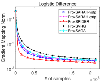
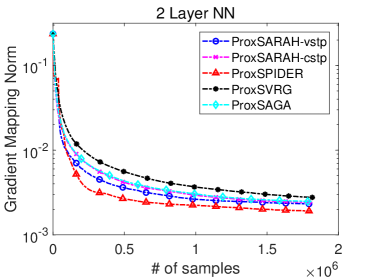
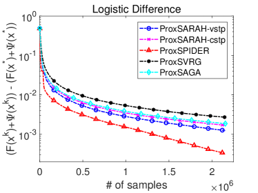
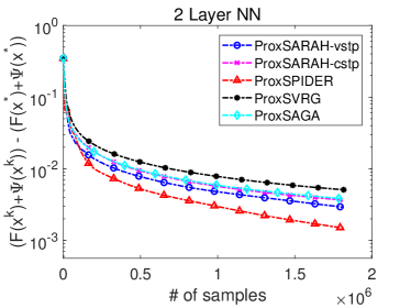
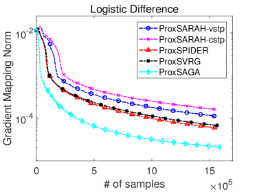
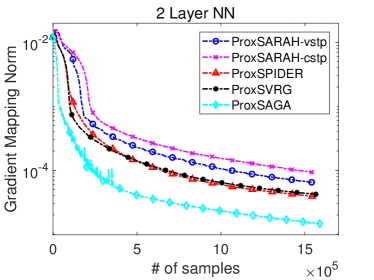
where $\{(a_{i},b_{i})\}_{i=1}^{N}$ are $N$ labeled examples with feature vectors $a_{i}\in\mathbf{R}^{d}$ and binary labels $y_{i}\in\{-1,,+1\}$. Specifically, we consider two different loss functions: the logistic difference loss $\ell_{ld}(t,b)=\log\big{(}1+e^{-bt}\big{)}-\log\big{(}1+e^{-bt-1}\big{)}$, and the 2 layer neural network loss $\ell_{nn}(t,b)=\big{(}1-\frac{1}{1+e^{-bt}}\big{)}^{2}$. For the $\ell_{1}$-norm penalty, we set $\beta=1/N$.

This is a standard one-level finite-sum problem, corresponding to the case of $m=1$ in (2). We compare the ProxSPIDER method (Algorithm 2) with the ProxSARAH algorithm [26]. ProxSARAH can be implemented with two schemes: for the variable stepsize scheme (Theorem 5, [26]) we use the name ProxSARAH-vstp; for the constant stepsize scheme (Theorem 6, [26]) we call it ProxSARAH-cstp. We also include the SVRG and SAGA estimator with normalized stepsize rule as described in Section 3.3 and 3.4 respectivley, which we call ProxSVRG and ProxSAGA.

Figure 1: Experiments on sparse binary classification on mnist dataset, $\beta=1/12691$.

The parameter setting (batch size, epoch length, etc.) of ProxSARAH-vstp and ProxSARAH-cstp are made to be consistent with the ProxSARAH-A-v1 and ProxSARAH-v1 in [26] where each mini-batch consists of only 1 sample, this is the parameter setting that yields the best empirical performance in [26]. For ProxSPIDER, we set both the batchsize and epoch length to be $\big{\lceil}\sqrt{N}\big{\rceil}$. For ProxSVRG and ProxSAGA, we set the batchsize to be $\big{\lceil}N^{\frac{2}{3}}\big{\rceil}$, the epoch length to be $\big{\lceil}N^{\frac{1}{3}}\big{\rceil}$. Finally, for ProxSPIDER, ProxSVRG and ProxSAGA, we use a variable sequence $\epsilon_{k}$ as in NPAG (Algorithm 1 and set $\epsilon_{k}=10/\sqrt{k}$.

First, we compare these methods over the mnist data sets. To fit the binary classification problems, we extract the data of two arbitrary digits, which are 1 and 9 in our experiments. This subset of mnist consists $N=12691$ data points. For the ProxSARAH-vstp and ProxSARAH-cstp, the parameter to be tuned is the estimator of the Lipschtiz constant $L$. The smaller $L$ is, the larger the stepsize is. For the ProxSPIDER, ProxSVRG and ProxSAGA, the parameter to be tuned is the stepsize $\eta$, which corresponds to $1/L$ in this experiment. We choose $L$ among $\{0.01,0.1,1,10\}$ and it turns out that $L=1$ works best for ProxSARAH-vstp and ProxSARAH-cstp for both loss functions. We choose $\eta$ among $\{0.1,1,10,100\}$ and it turns out that $\eta=1$ works best for ProxSIDER, ProxSVRG and ProxSAGA. These choices are consistent with the relationship $\eta=1/L$.

Figure 1 shows the norm of the gradient mapping and objective value gap of different methods. For all the compared methods, the curves are averaged over 20 runs of the algorithm. It can be seen that these different methods have similar performance, with ProxSVRG and ProxSAGA slightly worse and ProxSPIDER slightly better than other methods. In theory ProxSARAH and ProxSPIDER have the same sampling complexity, and the empirical results are consistent with the theory. Since the plots are very similar for the norm of gradient mapping and the objective value gap, we will only present plots of the gradient mapping norms for the rest of the experiments.

We also conduct our experiment on the rcv1.binary dataset, which is a medium sized dataset with $N=20242$ data points and each data point has $d=47236$ features. The parameters are chosen in a similar way to the experiments on mnist dataset. In particular, $L=0.01$ works best for ProxSARAH-vstp and ProxSARAH-cstp for both loss functions and $\eta=100$ works best for ProxSIDER, ProxSVRG and ProxSAGA (again we have $\eta=1/L$). Figure 2 shows the results of comparison. In this particular case, ProxSAGA perform the best despite a worse sample complexity in theory.

Figure 2: Experiments on sparse binary classification on rcv1 dataset, $\beta=1/20242$.

5.2 Sparse portfolio selection problem

In this section, we present the numerical results for a risk-averse portfolio optimization problems, which is a common benchmark example used in many stochastic composite optimization methds ($e.g.$, [16, 41, 42, 21]). Consider the scenario where $d$ assets can be invested during the time periods $\{1,...,N\}.$ We denote the per unit payoff vector at time $i$ by $r_{i}:=[r_{i,1},...,r_{i,d}]^{T}$, with $r_{i,j}$ being the per unit payoff of asset $j$ at time period $i$. Let $x\in\mathbf{R}^{d}$ be the decision variable, where the $j$-th component $x_{j}$ represents the amount of investment to asset $j$ throughout the $N$ time period, for $j=1,...,d.$

In the portfolio optimization problems, our aim is to maximize the average payoff over $N$ periods. However, a penalty is imposed on the variance of the payoff across the $N$ periods, which accounts for the risk of the investment. In addition, we also apply an $\ell_{1}$ penalty to impose sparsity on the portfolio $x$, which gives the following formulation:

$$\mathop{\textrm{maximize}}_{x\in\mathbf{R}^{d}}\mathbf{E}\big{[}\langle r_{\xi},x\rangle\big{]}-\lambda\mathbf{Var}(\langle r_{\xi},x\rangle)-\beta\|x\|_{1},$$

where the random variable $\xi$ follows the uniform distribution over $\{1,...,N\}$. Using the identity that $\mathbf{Var}(X)=\mathbf{E}[X^{2}]-\mathbf{E}[X]^{2}$, the problem can be reformulated as

$$\mathop{\textrm{minimize}}_{x\in\mathbf{R}^{d}}\mathbf{E}\big{[}\lambda\cdot\langle r_{\xi},x\rangle^{2}-\langle r_{\xi},x\rangle\big{]}-\lambda\cdot\mathbf{E}\big{[}\langle r_{\xi},x\rangle\big{]}^{2}+\beta\|x\|_{1}.$$ (50)

If we set $f_{1,\xi}(x):\mathbf{R}^{d}\mapsto\mathbf{R}^{2}=[\langle r_{\xi},x\rangle\,\,\langle r_{\xi},x\rangle^{2}]^{T}$, $f_{2,\xi_{2}}(y,z):\mathbf{R}^{2}\mapsto\mathbf{R}\equiv-y-\lambda y^{2}+\lambda z$, and $\Psi(x)=\beta\|x\|_{1},$ then (50) becomes a special case of (1) with $m=2$.

In the experiments, we compare our method with the C-SAGA algorithm [41], the CIVR and CIVR-adp algorithms [42], and the VRSC-PG algorithm [16]. We test these algorithms with the real world portfolio datasets from Keneth R. French Data Library. The first dataset is named Industrial-38, which contains 38 industrial assets payoff over 2552 consecutive time periods; and the second dataset is named Industrial-49, and contains 49 industrial assets over 24400 consecutive time periods. For both datasets, we set $\lambda=0.2$ and $\beta=0.01$ in problem (50). All the curves are averaged over 20 runs of the methods and are plotted against the number of samples of the component function and gradient evaluations.

Figure 3: Numerical experiments on the sparse portfolio optimization problem.

Figure 4: Experiments on Industrial-38 datasets using different step size parameter $\eta$.

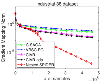
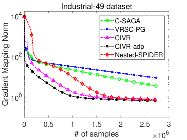
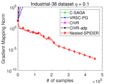
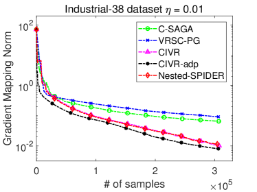
For these experiments, CIVR and Nested-SPIDER both take the batch size of $\lceil N^{1/2}\rceil$; CIVR-adp takes the adaptive batch size of $S_{k}=\lceil\min\{10k+1,N^{1/2}\}\rceil$; VRSC-PG and C-SAGA both take the batch size of $\lceil N^{2/3}\rceil$. For all these methods, their stepsizes $\eta$ are chosen as the best from $\{0.0001,0.001,0.01,0.1,1\}$ by experiments. In addition, we set $\epsilon_{k}=C/\sqrt{k}$ for Nested-SPIDER with $C$ chosen from $\{0.1,1,10,50\}$ by experiments. For the Industrial-38 dataset, $\eta=0.01$ works best for CIVR, CIVR-adp, C-SAGA and VRSC-PG, and $\eta=0.1$ and $C=1$ work best for Nested-SPIDER. For the Industrial-49 dataset, $\eta=0.0001$ works best for all five tested algorithms and $C=50$ works best for the Nested-SPIDER algorithm.

Figure 3 shows that for the Industrial-49 dataset, the CIVR-adp and CIVR perform the best. However, Nested-SPIDER quickly catches up with them after a slightly slower early stage, which is due to the relatively restrictive stepsizes caused by normalization (in early stages of the algorithm). On the contrary, Nested-SPIDER converges much faster than all other methods in the Industrial-38 dataset because the normalization step enables us to exploit a significantly larger stepsizes (in later stages of the algorithm), under which all the other methods diverge. In Figure 4, we show the following behavior of the Nested-SPIDER on Industrial-38. On the left, we set $\eta=0.1$ for all the algorithms and $C=1$ for Nested-SPIDER. All methods except for Nested-SPIDER diverge. On the right, we set $\eta=0.01$ for all the algorithms and $C=50$ for Nested-SPIDER. In this case, Nested-SPIDER behaves almost identical to CIVR.

6 Conclusion

We have proposed a normalized proximal approximate gradient (NPAG) method for solving multi-level composite stochastic optimization problems. The approximate gradients at each iteration are obtained via nested variance reduction using the SARAH/Spider estimator. In order to find an approximate stationary point where the expected norm of its gradient mapping is less than $\epsilon$, the total sample complexity of our method is $O(\epsilon^{-3})$ in the expectation case, and $O(N+\sqrt{N}\epsilon^{-2})$ in the finite-sum case where $N$ is the total number of functions across all composition levels. In addition, the dependence of the sample complexity on the number of composition levels is polynomial, rather than exponential as in previous work. Our results rely on a uniform Lipschitz condition on the composite mappings and functions, which is stronger than the mean-squared Lipschitz condition required for obtaining similar complexities for single-level stochastic optimization.

The NPAG method extends the Spider-SFO method [13] to the proximal setting and for solving multi-level composite stochastic optimization problems. In particular, requiring a uniform bound on the MSEs of the approximate gradients allows separate analysis of the optimization algorithm and variance reduction. In addition, the uniform bound on the step lengths at each iteration is the key to enable our analysis of nested variance reduction. More flexible rules for choosing the step sizes or step lengths have been developed to obtain similar sample complexities for single-level stochastic or finite-sum optimization problems, especially those used in the Spider-Boost [37] and Prox-SARAH [26] methods. It is likely that such step size rules may also be developed for multi-level problems, although their complexity analysis may become much more involved.

Appendix A Proof of Lemma 4.2

Proof.

Under Assumption 4.1.(a), it is straightforward to show that $f_{i}=\mathbf{E}_{\xi_{i}}f_{i,\xi_{i}}$ is $\ell_{i}$-Lipschitz and its gradient $f^{\prime}_{i}=\mathbf{E}_{\xi_{i}}f^{\prime}_{i,\xi_{i}}$ is $L_{i}$-Lipschitz. Recall the definitions $F_{i}=f_{i}\circ f_{i-1}\circ\cdots\circ f_{1}$ for $i=1,\ldots,m$. By the chain rule, we have

$$\|F^{\prime}(x)-F^{\prime}(y)\|$$

$$= \bigl{\|}[f_{1}^{\prime}(x)]^{T}\cdots[f_{m-1}^{\prime}(F_{m-2}(x))]^{T}f_{m}^{\prime}(F_{m-1}(x))$$

$$~{}-~{}[f_{1}^{\prime}(y)]^{T}\cdots[f_{m-1}^{\prime}(F_{m-2}(y))]^{T}f_{m}^{\prime}(F_{m-1}(y))\bigr{\|}$$

$$\leq \big{\|}[f_{1}^{\prime}(x)]^{T}\!\!\cdots[f_{m\!-\!1}^{\prime}(F_{m\!-\!2}(x))]^{T}\!f_{m}^{\prime}(F_{m\!-\!1}(x))-[f_{1}^{\prime}(y)]^{T}[f_{2}^{\prime}(F_{1}(x))]^{T}\!\!\cdots f_{m}^{\prime}(F_{m\!-\!1}(x))\big{\|}$$

$$+\cdots$$

$$+\big{\|}[f_{1}^{\prime}(y)]^{T}\!\!\cdots\![f_{m\!-\!1}^{\prime}(F_{m\!-\!2}(y))]^{T}\!f_{m}^{\prime}(F_{m\!-\!1}(x))-[f_{1}^{\prime}(y)]^{T}[f_{2}^{\prime}(F_{1}(y))]^{T}\!\!\cdots\!f_{m}^{\prime}(F_{m\!-\!1}(y))\big{\|}$$

$$\leq L_{1}\mathop{\textstyle\prod}_{r\neq 1}\ell_{r}\|x-y\|+L_{2}\mathop{\textstyle\prod}_{r\neq 2}\ell_{r}\|F_{1}(x)-F_{1}(y)\|+...+L_{m}\mathop{\textstyle\prod}_{r\neq m}\ell_{r}\|F_{m}(x)-F_{m}(y)\|.$$

On the other hand, we have for any $x$ and $y$ that

$$\|F_{i}(x)-F_{i}(y)\| = \|f_{i}(F_{i-1}(x))-f_{i}(F_{i-1}(y))\|$$

$$\leq \ell_{i}\|F_{i-1}(x)-F_{i-1}(y)\|\leq\mathop{\textstyle\prod}_{r=1}^{i}\ell_{r}\|x-y\|.$$

Therefore $F_{i}$ is $\ell_{F}$-Lipschitz with $\ell_{F}=\mathop{\textstyle\prod}_{i=1}^{m}\ell_{i}$. Substituting these Lipschitz constants into the bound of $\|F^{\prime}(x)-F^{\prime}(y)\|$ yields

$$\|F^{\prime}(x)-F^{\prime}(y)\|\leq\left(\sum_{i=1}^{m}L_{i}\biggl{(}\mathop{\textstyle\prod}_{r=1}^{i-1}\ell_{r}\biggr{)}^{2}\cdot\biggl{(}\mathop{\textstyle\prod}_{r=i+1}^{m}\ell_{r}\biggr{)}\right)\|x-y\|,$$

which gives the expression of $L_{F}$ in (36). ∎

References

- [1] Zeyuan Allen-Zhu. Natasha: Faster non-convex stochastic optimization via strongly non-convex parameter. In Proceedings of the 34th International Conference on Machine Learning (ICML), volume 70 of Proceedings of Machine Learning Research, pages 89–97, Sydney, Australia, 2017.
- [2] Zeyuan Allen-Zhu. Natasha 2: Faster non-convex optimization than SGD. In Advances in Neural Information Processing Systems 31, pages 2675–2686. Curran Associates, Inc., 2018.
- [3] Zeyuan Allen-Zhu and Elad Hazan. Variance reduction for faster non-convex optimization. In Proceedings of the 33rd International Conference on Machine Learning, pages 699–707, 2016.
- [4] Zeyuan Allen-Zhu and Yang Yuan. Improved SVRG for non-strongly-convex or sum-of-non-convex objectives. In Proceedings of the 33rd International Conference on International Conference on Machine Learning (ICML), pages 1080–1089, 2016.
- [5] Amir Beck. First-Order Methods in Optimization. MOS-SIAM Series on Optimization. SIAM, 2017.
- [6] Jose Blanchet, Donald Goldfarb, Garud Iyengar, Fengpei Li, and Chaoxu Zhou. Unbiased simulation for optimizing stochastic function compositions. Preprint, arXiv:1711.07564, 2017.
- [7] Christoph Dann, Gerhard Neumann, and Jan Peters. Policy evaluation with temporal differences: a survey and comparison. Journal of Machine Learning Research, 15(1):809–883, 2014.
- [8] Aaron Defazio, Francis Bach, and Simon Lacoste-Julien. SAGA: A fast incremental gradient method with support for non-strongly convex composite objectives. In Advances in Neural Information Processing Systems 27, pages 1646–1654, 2014.
- [9] Ofer Dekel, Ran Gilad-Bachrach, Ohad Shamir, and Lin Xiao. Optimal distributed online prediction using mini-batches. Jorunal of Machine Learning Research, 13:165–202, 2012.
- [10] Darinka Dentcheva, Spiridon Penev, and Andrzej Ruszczyński. Statistical estimation of composite risk functionals and risk optimization problems. Annals of the Institute of Statistical Mathematics, 69(4):737–760, 2017.
- [11] Dmitriy Drusvyatskiy and Adrian S. Lewis. Error bounds, quadratic growth, and linear convergence of proximal methods. Mathematics of Operations Research, 43(3):919–948, 2018.
- [12] Y. Ermoliev. Methods of Stochastic Programming. Monographs in Optimization and OR. Nauka, Moscow, 1976.
- [13] Cong Fang, Chris Junchi Li, Zhouchen Lin, and Tong Zhang. Spider: Near-optimal non-convex optimization via stochastic path-integrated differential estimator. In Advances in Neural Information Processing Systems 31, pages 689–699. Curran Associates, Inc., 2018.
- [14] Saeed Ghadimi and Guanghui Lan. Stochastic first- and zeroth-order methods for nonconvex stochastic programming. SIAM Journal on Optimization, 23(4):2341–2368, 2013.
- [15] Saeed Ghadimi, Andrzej Ruszczyński, and Mengdi Wang. A single time-scale stochastic approximation method for nested stochastic optimization. Preprint, arXiv:1812.01094, 2018.
- [16] Zhouyuan Huo, Bin Gu, Ji Jiu, and Heng Huang. Accelerated method for stochastic composition optimization with nonsmooth regularization. In Proceedings of the 32nd AAAI Conference on Artificial Intelligence, pages 3287–3294, 2018.
- [17] A. N. Iusem, A. Jofré, R. I. Oliveira, and P. Phompson. Extragradient method with variance reduction for stochastic variational inequalities. SIAM Journal on Optimization, 27(2):686–724, 2017.
- [18] Rie Johnson and Tong Zhang. Accelerating stochastic gradient descent using predictive variance reduction. In Advances in Neural Information Processing Systems 26, pages 315–323, 2013.
- [19] J. Koshal, A. Nedić, and U. B. Shanbhag. Regularized iterative stochastic approximation methods for stochastic variational inequality problems. IEEE Transactions on Automatic Control, 58(3):594–609, 2013.
- [20] Xiangru Lian, Mengdi Wang, and Ji Liu. Finite-sum composition optimization via variance reduced gradient descent. In Proceedings of the 20th International Conference on Artificial Intelligence and Statistics (AISTATS), pages 1159–1167, 2017.
- [21] Tianyi Lin, Chenyou Fan, Mengdi Wang, and Michael I Jordan. Improved oracle complexity for stochastic compositional variance reduced gradient. Preprint, arXiv:1806.00458, 2018.
- [22] Yurii Nesterov. Gradient methods for minimizing composite functions. Mathematical Programming, 140(1):125–161, 2013.
- [23] Yurii Nesterov. Lectures on Convex Optimization. Springer, 2nd edition, 2018.
- [24] Lam M. Nguyen, Jie Liu, Katya Scheinberg, and Martin Takáč. SARAH: A novel method for machine learning problems using stochastic recursive gradient. In Proceedings of the 34th International Conference on Machine Learning (ICML), volume 70 of PMLR, pages 2613–2621, 2017.
- [25] Lam M. Nguyen, Marten van Dijk, Dzung T. Phan, Phuong Ha Nguyen, Tsui-Wei Weng, and Jayant R. Kalagnanam. Finite-sum smooth optimization with SARAH. arXiv:1901.07648, 2019.
- [26] Nhan H. Pham, Lam M. Nguyen, Dzung T. Phan, and Quoc Tran-Dinh. ProxSARAH: An efficient algorithmic framework for stochastic composite nonconvex optimization. Preprint, arXiv:1902.05679, 2019.
- [27] Sashank J. Reddi, Ahmed Hefny, Suvrit Sra, Barnabas Poczos, and Alex Smola. Stochastic variance reduction for nonconvex optimization. In Proceedings of The 33rd International Conference on Machine Learning, volume 48 of Proceedings of Machine Learning Research, pages 314–323, New York, New York, USA, 2016.
- [28] Sashank J Reddi, Suvrit Sra, Barnabás Póczos, and Alex Smola. Fast incremental method for smooth nonconvex optimization. In 2016 IEEE 55th Conference on Decision and Control (CDC), pages 1971–1977. IEEE, 2016.
- [29] Sashank J Reddi, Suvrit Sra, Barnabás Póczos, and Alexander J Smola. Proximal stochastic methods for nonsmooth nonconvex finite-sum optimization. In Advances in Neural Information Processing Systems 29, pages 1145–1153, 2016.
- [30] R. Tyrrell Rockafellar. Convex Analysis. Princeton University Press, 1970.
- [31] R. Tyrrell Rockafellar. Coherent approaches to risk in optimization under uncertainty. INFORMS TutORials in Operations Research, 2007.
- [32] Nicolas L. Roux, Mark Schmidt, and Francis R. Bach. A stochastic gradient method with an exponential convergence _rate for finite training sets. In Advances in Neural Information Processing Systems 25, pages 2663–2671. Curran Associates, Inc., 2012.
- [33] Andrzej Ruszczyński. Advances in risk-averse optimization. INFORMS TutORials in Operation Research, 2013.
- [34] Richard S Sutton and Andrew G Barto. Reinforcement Learning: An Introduction. MIT Press, Cambridge, MA, 1998.
- [35] Mengdi Wang, Ethan X Fang, and Han Liu. Stochastic compositional gradient descent: algorithms for minimizing compositions of expected-value functions. Mathematical Programming, 161(1-2):419–449, 2017.
- [36] Mengdi Wang, Ji Liu, and Ethan Fang. Accelerating stochastic composition optimization. Journal of Machine Learning Research, 18(105):1–23, 2017.
- [37] Zhe Wang, Kaiyi Ji, Yi Zhou, Yingbin Liang, and Vahid Tarokh. SpiderBoost: A class of faster variance-reduced algorithms for nonconvex optimization. Preprint, arXiv:1810.10690, 2018.
- [38] Lin Xiao and Tong Zhang. A proximal stochastic gradient method with progressive variance reduction. SIAM Journal on Optimization, 24(4):2057–2075, 2014.
- [39] Shuoguang Yang, Mengdi Wang, and Ethan X. Fang. Multilevel stochastic gradient methods for nested composition optimization. SIAM Journal on Optimization, 29(1):616–659, 2019.
- [40] Xiaoyong Yuan, Pan He, Qile Zhu, and Xiaolin Li. Adversarial examples: Attacks and defenses for deep learning. IEEE Transactions on Neural Networks and Learning Systems, 30(9):2805–2824, 2019.
- [41] Junyu Zhang and Lin Xiao. A composite randomized incremental gradient method. In Proceedings of the 36th International Conference on Machine Learning (ICML), number 97 in Proceedings of Machine Learning Research (PMLR), Long Beach, California, 2019.
- [42] Junyu Zhang and Lin Xiao. A stochastic composite gradient method with incremental variance reduction. In Advances in Neural Information Processing Systems 32, pages 9078–9088. Curran Associates, Inc., 2019.
- [43] Dongruo Zhou, Pan Xu, and Quanquan Gu. Stochastic nested variance reduced gradient descent for nonconvex optimization. In Advances in Neural Information Processing Systems 31, pages 3921–3932. Curran Associates, Inc., 2018.