CorNet: Generic 3D Corners for 6D Pose Estimation of
New Objects without Retraining

Abstract

We present a novel approach to the detection and 3D pose estimation of objects in color images. Its main contribution is that it does not require any training phases nor data for new objects, while state-of-the-art methods typically require hours of training time and hundreds of training registered images. Instead, our method relies only on the objects’ geometries. Our method focuses on objects with prominent corners, which covers a large number of industrial objects. We first learn to detect object corners of various shapes in images and also to predict their 3D poses, by using training images of a small set of objects. To detect a new object in a given image, we first identify its corners from its CAD model; we also detect the corners visible in the image and predict their 3D poses. We then introduce a RANSAC-like algorithm that robustly and efficiently detects and estimates the object’s 3D pose by matching its corners on the CAD model with their detected counterparts in the image. Because we also estimate the 3D poses of the corners in the image, detecting only 1 or 2 corners is sufficient to estimate the pose of the object, which makes the approach robust to occlusions. We finally rely on a final check that exploits the full 3D geometry of the objects, in case multiple objects have the same corner spatial arrangement. The advantages of our approach make it particularly attractive for industrial contexts, and we demonstrate our approach on the challenging T-LESS dataset.

1 Introduction

3D object detection and pose estimation are of primary importance for tasks such as robotic manipulation, virtual and augmented reality and they have been the focus of intense research in recent years, mostly due to the advent of Deep Learning based approaches and the possibility of using large datasets for training such methods. Methods relying on depth data acquired by depth cameras are robust [15, 9]. Unfortunately, active depth sensors are power hungry or sometimes it is not possible to use them.

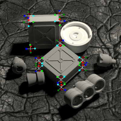
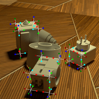
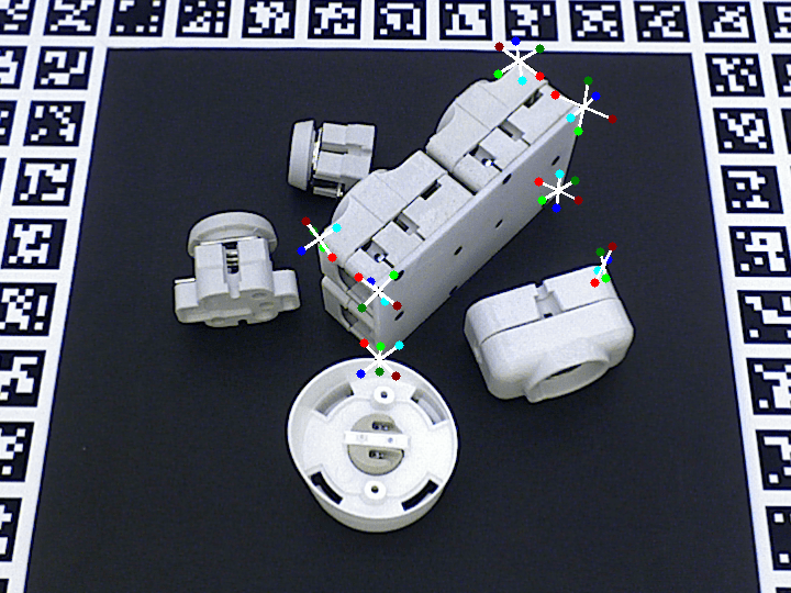
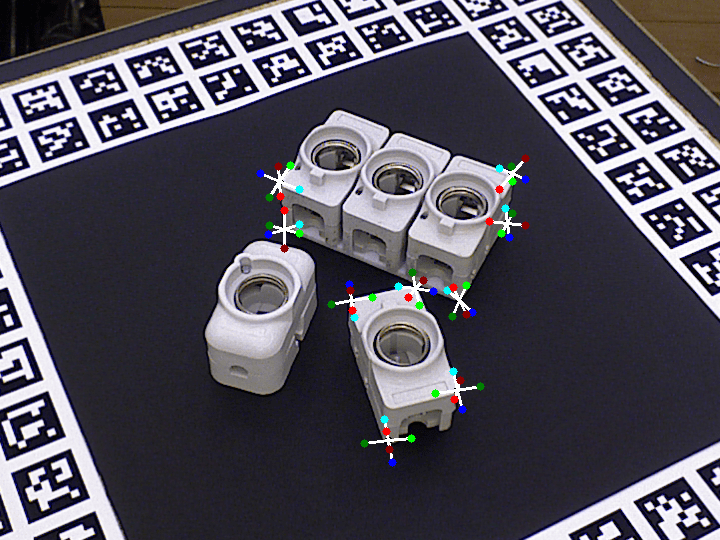
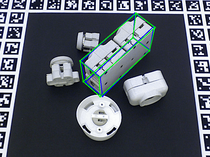
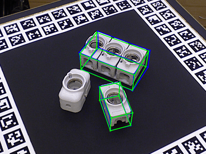
Figure 1: Given a small set of objects from the T-LESS dataset [17], we learn to detect corners of various appearances and shapes and to estimate their 3D poses using synthetic renderings (first row). Then, given only the CAD model of new objects with corners, we can detect these objects and estimate their 3D poses, without any new training phase (second and third rows). The green bounding boxes correspond to the ground truth poses and the blue bounding boxes to the poses estimated with our method.

It is therefore often desirable to rely on color images, and many methods to do so have been proposed recently [19, 25, 31, 18, 35, 24]. However, the success of these methods can be attributed to supervised Machine Learning approaches, and for each new object, these methods have to be retrained on many different images of this object. Even if domain transfer methods allow for training such methods with synthetic images [16, 19, 30] instead of real ones [2, 39, 10, 22, 33, 20, 26, 37] at least to some extent, such training sessions take time, and it is highly desirable to avoid them in practice.

In this paper, we propose a method that does not require additional learning nor training images for new objects: We consider a scenario where CAD models for the target objects exist, but not necessarily training images. This is often the case in industrial settings, where an object is built from its CAD model. We rely on corners which we learn to detect and estimate the 3D poses during an offline stage. Our approach focuses on industrial objects. Industrial objects are often made of similar parts, and corners are a dominant common part. Detecting these corners and determining their 3D poses is the basis for our approach. We follow a deep learning approach and train FasterRCNN on a small set of objects to detect corners and predict their 3D poses.

We use the representation of 3D poses introduced by [7]: The 3D pose of a corner is predicted in the form of a set of 2D reprojections of 3D virtual points. This is convenient for our purpose, since multiple corners can be easily combined to compute the object pose when using this representation. However, we need to take care of a challenge that arises with corners, and that was ignored in [7]: Because of its symmetries, the 3D pose of a corner is often ambiguous, and defined only up a set of rigid rotations. We therefore introduce a robust and efficient algorithm that considers the multiple possible 3D poses of the detected corners, to finally estimate the 3D poses of the new objects.

In the remainder of the paper, we review the state-of-the-art on 3D object pose estimation from images, describe our method, and evaluate it on the T-LESS dataset, which is made of very challenging objects and sequences.

2 Related Work

In this section, we first review recent work on 3D object detection and pose estimation from color images. We also review works on transfer learning for 3D pose estimation, as it is a common approach to decrease the number of real training images.

2.1 3D Object Detection and Pose Estimation from Color Images

Several recent works extend on deep architectures developed for 2D object detection by also predicting the 3D pose of objects. [19] trained the SSD architecture [21] to also predict the 3D rotations of the objects, and the depths of the objects. To improve robustness to partial occlusions, PoseCNN [35] segments the objects’ masks and predicts the objects’ poses in the form of a 3D translation and a 3D rotation. Also focusing on occlusion handling, PVNet [24] proposed a network that for each pixel regresses an offset to predefined keypoints. Deep-6DPose [8] relies on Mask-RCNN [14]. Yolo3D [31] relies on Yolo [27] and predicts the object poses in the form of the 2D projections of the corners of the 3D bounding boxes, instead of a 2D bounding box. [25] also used this representation to predict the 3D pose of objects, and shows how to deal with some of the ambiguities of the objects from T-Less—however it does not provide a general solution. Some methods [19, 16, 30] use synthetic training images generated from CAD models, but for each new model, they need to retrain their network, or a new one.

Somewhat related to our approach, [18, 4, 38, 24] first predict the 3D coordinates of the image locations lying on the objects, in the object coordinate system, and predict the 3D object pose through hypotheses sampling with preemptive RANSAC. Instead of predicting the 3D coordinates of 2D locations, [7] predicts the 2D projections of 3D virtual points attached to object parts. The advantage of this approach is its robustness to partial occlusions, as it is based on parts, and the fact that the detected parts can be used easily together to compute the 3D pose of the target object. In this paper, we rely on a similar representation of parts, but extends it to deal with ambiguities, and show how to use it to detect unknown objects without retraining.

All these works require extensive training sessions for new objects, which is what we avoid in our approach. Previous works, based on templates, also aim at avoiding such training sessions. For example, [15] proposes a descriptor for object templates, based on image and depth gradients. Deep Learning has also been applied to such approach, by learning to compute a descriptor from pairs or triplets of object images [34, 1, 36, 5]. Like ours, these approaches do not require re-training, as it only requires to compute the descriptors for images of the new objects. However, it requires many images from points of view sampled around the object. It may be possible to use synthetic images, but then, some domain transfer has to be performed. But the main drawback of this approach is the lack of robustness to partial occlusions, as the descriptor is computed for whole images of objects. It is also not clear how it would handle ambiguities, as it is based on metric learning on images. In fact, such approach has been demonstrated on the LineMod, which is made of relatively simple objects, and never on the T-Less dataset, which is much more challenging.

2.2 Transfer Learning for 3D Pose Estimation

Another approach to limit the number of real training images is to rely on synthetic images, which can be rendered when a CAD model is available as we assume here. This is a very popular approach, which requires domain transfer between synthetic and real images. Domain transfer between images from different datasets is a common problem in computer vision [12, 29, 6, 2, 39, 10, 22, 33, 20, 26, 37], and we focus here only on works related to 3D pose estimation.

Generative Adversarial Networks (GANs) [11] have been used to generate training images [3, 23, 2, 39, 10, 22, 33, 20, 26, 37], by making synthetic images closer to real images. However, they need to have access to target domain data and usually overfit to them and would not generalize well to new domains. Differently, [37] chose to make real depth images closer to clean synthetic depth images. It requires however careful augmentation to create realistic synthetic depth maps. Because synthetic depth maps are easier to render than color images, [26] proposes to learn a mapping between features for depth maps and features for color images using an RGB-D camera. Another interesting approach is domain randomization [32], which generates synthetic training images with random appearance, by varying the object textures and rendering parameters, to improve generalization. AAE [30] presents another domain randomization approach based on autoencoders to train pose estimation network from CAD models.

Even if these works allow to reduce the number of real images required for training, or to completely get rid of them, they still require a training session for new objects, which is what we avoid entirely with our approach.

3 Approach

We describe our approach in this section. We first describe how we learn to detect corners and predict their 3D poses. We then present our algorithm to estimate the 3D poses of new objects in an input image, from the corners detected in this image.

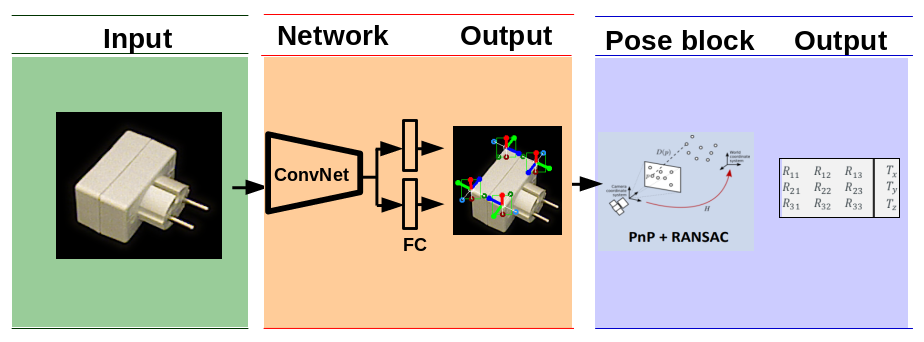
Figure 2: Overview of our approach. We modified FasterRCNN to detect generic corners in images and predict their 3D poses. Our pose estimation algorithm, which is an extension of RANSAC, estimates the 3D poses of full objects from these detections.

3.1 Corner Detection and 3D Pose Estimation

We use the representation of the 3D pose of a part introduced in [7] to represent the 3D pose of our corners. This representation is made of the 2D reprojections of a set of 3D control points. Its main advantage is that it is easy to combine the 3D poses of multiple parts to compute the 3D pose of the object by solving a P$n$P problem [13]. These control points are only “virtual”, in the sense they do not have to correspond to specific image features. As shown in Fig. 3, we consider seven 3D control points for each part, arranged to span 3 orthogonal directions and the center of the part, as in [7].

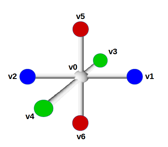
(a)	(b)

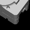
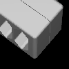
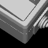
(c)

Figure 3: 3D pose representation of an object part from [7]. (a) Seven 3D control points arranged to span 3 orthogonal directions are assigned to each part. (b) Given an image patch of the part, [7] predicts the 2D reprojections of these control points, and computes the 3D pose of the objects from these 3D-2D correspondences. The first difference with [7] is that our corners are generic in the sense that they can correspond to corners of various shapes and appearances, as corners from different objects can actually be different (c), while [7] considers parts from object instances. This allows us to consider new objects without retraining. The other difference is that we need to handle the pose ambiguities of corners (due to their symmetries), which was not considered in [7]. This is done in our 3D pose estimation algorithm.

While [7] performed detection and pose prediction with two separate networks, we rely on the Faster-RCNN framework [28] as it is common practice now for various problems: We kept the original architecture to obtain region proposals that correspond to parts and added a specific branch to predict the 2D coordinates of each control point. This branch is implemented as a fully connected two-layer perceptron. The size of its output is $2\times N_{v}$, where $N_{v}$ is the number of control points for a detected corner, and with $N_{v}=7$ in practice. For training, we used the default hyperparameters used in [28] and the same loss function to predict the object class (corner vs background). We also added to the global loss term, a squared loss for training the predictions of the reprojections of the control points.

To train FasterRCNN, we used a small number of objects exhibiting different types of corners, shown in Fig. 3(c), and created synthetic images of these objects for training. Two examples of these images are shown on the first row of Fig. 1. These images are created by randomly placing the training objects in a simple scene made of a plane randomly textured, and randomly lighted. In practice, we noticed that we did not need to apply transfer learning to take care of the domain gap between our synthetic images and the real test images of T-LESS. This is probably due to the fact that we consider only local parts of the images, and because the test images of T-LESS are relatively noise-free. Given the CAD models of these objects we can select the control points in 3D and project them with the ground truth pose. In this way, we obtain the 2D ground truths reprojections of the control points needed to train the network.

3.2 Ambiguities between Corner Poses and How to Handle Them

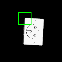
Figure 4: The same corner can look the same under different 3D poses. This implies that it is possible to predict the 3D pose of a corner only up to some rigid motions.

As shown in Fig. 4, many ambiguities may happen when trying to predict the 3D pose of a corner from its appearance. These ambiguities do not happen in the problems considered by [7], and are due to the symmetries of corners. If we ignore these ambiguities, we would consider only one pose among all the possible poses for each detected corner, which would result in missing new objects very often.

From the image of a corner, there are in general 3 possible 3D poses that correspond to this image, as shown in Fig. 5. Given one possible 3D pose ${\bf p}$, it is possible to generate the two other poses by applying rotations around the corner. In our case, since we represent the pose with the 2D reprojections of the virtual points, this can also be done by permuting properly the 2D reprojections. We therefore introduce 2 permutations $\Sigma_{1}$ and $\Sigma_{2}$ which operate on the 2D reprojections as depicted in Fig. 5. Given a pose predicted by FasterRCNN, we can generate the 2 other possible poses by applying $\Sigma_{1}$ and $\Sigma_{2}$. This is used in our pose estimation algorithm described in the next subsection.

Figure 5: Given the image of a corner, three arrangements of 3D virtual points are possible.

3.3 Pose Estimation Algorithm

We represent a new object to detect as a set $\mathcal{C}=\{\mathcal{C}_{1},..,\mathcal{C}_{N_{C}}\}$ of $N_{C}$ 3D corners. This can be done using only the CAD model of the object. Each corner is made of $N_{v}$ 3D virtual points: $\mathcal{C}_{i}=\{M_{i,1},..,M_{i,N_{v}}\}$ expressed in the object coordinate system.

From our FasterRCNN framework, given an input image, we obtain a set $\mathcal{D}=\{d_{1},\ldots,d_{N_{d}}\}$ of $N_{D}$ detected corners $d_{j}$. Each detected corner $d_{j}$ is made of $N_{v}$ predicted 2D reprojections: $d_{j}=[m_{j,1},\ldots,m_{j,N_{v}}]$.

The pseudocode for our detection and pose estimation algorithm is given as Alg. 1. To deal with the erroneous detected parts, we use the same strategy as RANSAC. By matching the detected corners $d_{j}$ with their 3D counterparts $\mathcal{C}_{i}$, it is possible to compute the 3D pose of the object using a PnP algorithm. Since each corner is represented by $N_{v}=7$ points, it is possible to compute the pose from a single match. As explained in Section 3.2, each detected corner can correspond to 3 possible arrangements of virtual points, and we apply $\Sigma_{1}$ and $\Sigma_{2}$ to the $m_{j,k}$ reprojections to generate the 3D possible poses for the detected corners.

In order to find the best pose among all these 3D possible poses, we compute a similarity score as the cross-correlation between the gradients of the image and the image gradients of the CAD model rendered under the 3D pose. We finally keep the pose with the largest similarity score as the estimated pose.

1:$\mathcal{C}\leftarrow\{C_{i}\}_{i}$, the set of 3D corners on the new object. Each 3D corner $C_{i}$ is made of 7 3D control points, expressed in the coordinate system of the new object.

2:$\mathcal{D}\leftarrow\{d_{j}\}_{j}$, the set of 2D detected corners in the input image. Each 2D corner $d_{j}$ is made of 7 2D image locations.

3:

4:procedure Pose_Estimation($\mathcal{C}$, $\mathcal{D}$)

5:     ${poses}\leftarrow[]$ $\triangleright$ Set of possible poses and their scores

6:     for $C\in\mathcal{C}$ do

7:         for $d\in\mathcal{D}$ do

8:             for $\Sigma\in\{I,\Sigma_{1},\Sigma_{2}\}$ do

9:                 $\text{corr}\leftarrow(C,\Sigma(d))$ $\triangleright$ 2D-3D correspondence

10:                 ${pose}\leftarrow\textsc{PnP}(\text{corr})$ $\triangleright$ 3D pose estimate

11:                 $nb_{\text{inliers}}\leftarrow\textsc{Compute\_Inliers}({pose},\mathcal{C},\mathcal{D})$

12:                 if $nb_{\text{inliers}}>\tau_{\text{inliers}}$ then

13:                     $\textsc{Refine}({pose},\mathcal{C},\mathcal{D})$ $\triangleright$ Compute pose using all the inliers

14:                     $s_{pose}\leftarrow\textsc{Score}({pose},\mathcal{C},\mathcal{D})$

15:                     Add $({pose},s_{pose})$ to ${poses}$                                             

16:     return ${pose}$ with best $s_{pose}$ in ${poses}$

17:

18:procedure Score(${pose}$, $\mathcal{C}$, $\mathcal{D}$)

19:    $s\leftarrow 0$

20:    $template\leftarrow ImageGradients(rendering(model,{pose})$

21:    $edges_{input}\leftarrow ImageGradients(input_{image})$

22:    $s\leftarrow Cross\_Correlation(edges_{input},template)$

23:    return $s$

Algorithm 1 Pose estimation algorithm

4 Evaluation

In this section, we present and discuss the results of our pose estimation algorithm. We first describe the metrics used in the literature and in this paper. Then, we show a quantitative analysis of object detection and pose estimation as well as qualitative results. All the results are computed on the challenging T-LESS dataset [17].

4.1 Metrics

To evaluate our method, we use the percentage of correctly predicted poses for each sequence and each object of interest, where a pose is considered correct based on the ADD metric. This metric is based on the average distance in 3D between the model points after applying the ground truth pose and the estimated one. A pose is considered correct if the distance is less than 10% of the object’s diameter.

4.2 Results

The complexity of the test scenes varies from several isolated objects on a clean background to very challenging ones with multiple instances of several objects with a high amount of occlusions and clutters. Only few previous works present results on the challenging T-LESS dataset [17]. To the best of our knowledge, the problem of pose estimation of new objects that have not been seen at training time has not been addressed yet.

In order to evaluate our method, we split the objects from T-LESS into two sets: One set of objects seen by the network during the training and one set of objects never seen and used for evaluation at testing time. More specifically, we train our network on corners extracted from Objects #6, #19, #25, #27 and #28 and test it on Objects #7, #8, #20, #26 and #29 on T-LESS test scenes #02, #03, #04, #06, #08, #10, #11, #12, #13, #14 and #15.

Scene: Obj	$AD\{D|I\}_{10\%}$	$AD\{D|I\}_{20\%}$	$AD\{D|I\}_{30\%}$	detection [$\%$]
02: 7	68.3	80.1	83.7	67.3
03: 8	57.9	72.5	78.7	76.3
04: 26	28.1	47.2	56.2	48.3
04: 8	21.2	53.0	68.2	35.7
06: 7	36.8	61.7	78.7	73.7
08: 20	10.0	40.4	56.1	34.1
10: 20	27.8	47.2	58.3	30.0
11: 8	58.8	74.9	85.3	74.3
12: 7	23.1	44.6	47.7	54.6
13: 20	26.6	57.3	69.0	52.9
15: 29	48.0	59.1	76.7	38.3
14: 20	10.0	24.6	31.6	44.0
Average	34.7($\pm$18.5)	55.2($\pm$15.2)	65.9($\pm$15.6)	52.5($\pm$16.2)

Table 1: Our quantitative results on T-Less test Scenes #02, #03, #04, #06, #08, #10, #11, #12, #13, #14, #15. Last column reports the detection accuracy. We consider the object to be detected if the $IoU$ between the rendering of the object with the pose estimate and with the ground truth is higher then $0.4$.

4.2.1 2D Detection

We first evaluate our method in terms of 2D detection. Even this task is challenging on the T-LESS dataset given our setting, as the objects are very similar to each others.

Most of previous works separate the detection task from the pose estimation. For example, in [25], the authors present a method that first detects objects through a segmentation approach and then use the corresponding crop of the image to estimate the pose. Some works only focus on pose estimation [30], and use the ground-truth crops of each objects of the scene to avoid the detection step.

In this work, we cannot access images of objects on which the pose estimation is done. Thus, it is not possible to train a separated object detection network or segmentation network to solve this problem. Our method returns directly the 3D poses of the objects. To evaluate the detection accuracy, we therefore use the 2D bounding boxes computed from the reprojections of the CAD models under the estimated 3D pose.

We report our detection accuracy in the last column of Table 1. The accuracy is measured in terms of Intersection over Union ($IoU$) between the rendering of the object with the estimated pose and the rendering of the object with the ground truth pose. An object is considered correctly detected in the frame if $IoU>0.4$. Our method succeeds an average of $52.5\%$ of good detection without any detection or segmentation priors.

4.2.2 3D Pose Estimation

We evaluate the pose estimation on images where the object of interest has been detected. For each object of our experiments, we compute the ADD metric presented above. Table 1 reports the scores for three percentages of object diameters. For symmetrical objects, we report the ADI metric instead of ADD. The object 3D orientation and translation along the x-and y-axes are typically well estimated. Most of the translation error is along the z-axis, as it is usually the case of other algorithms for 3D pose estimation from color images.

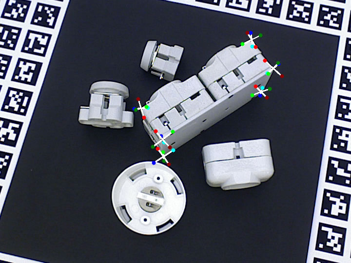
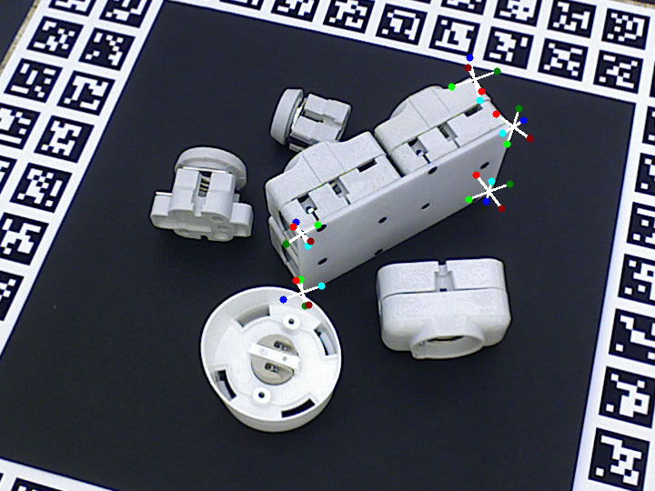
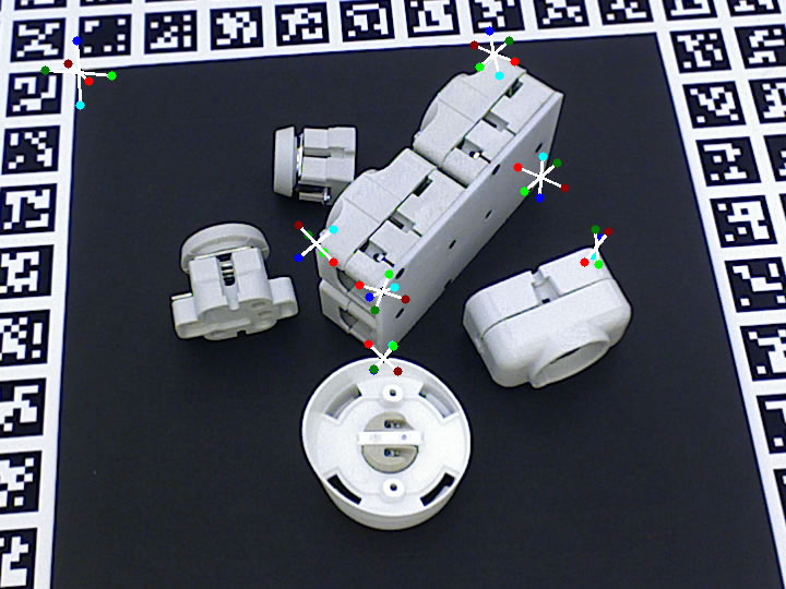
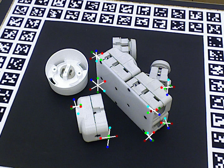
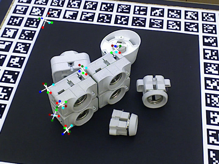
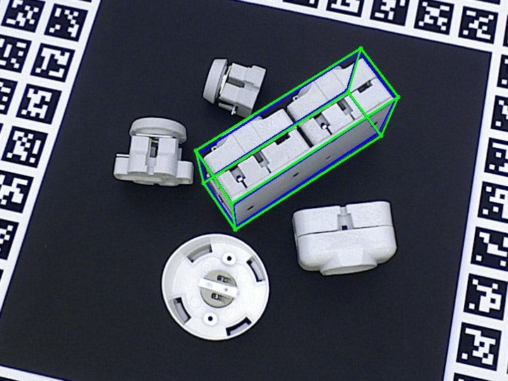
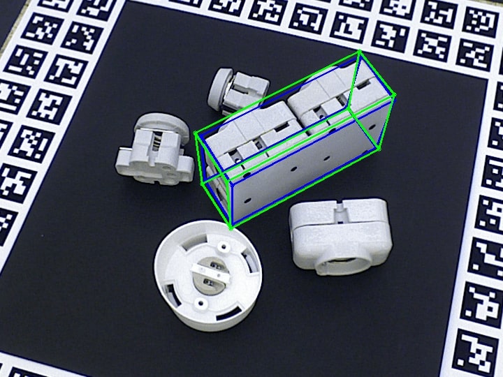
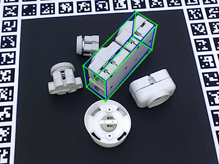
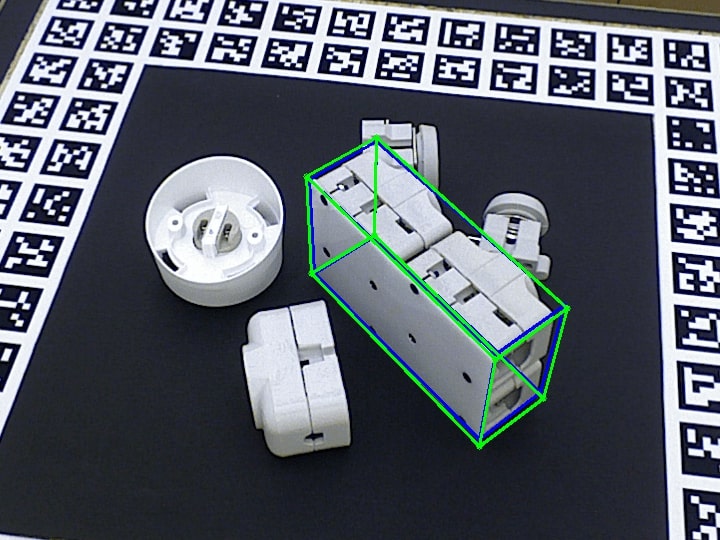
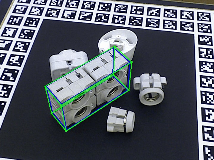
Figure 6: Some qualitative results on Object #8 in Scene #03 of the T-LESS dataset. First row: 2D detection results. Second row: 3D Pose Estimation results. Green and blue bounding boxes are the ground truth and estimated poses respectively.

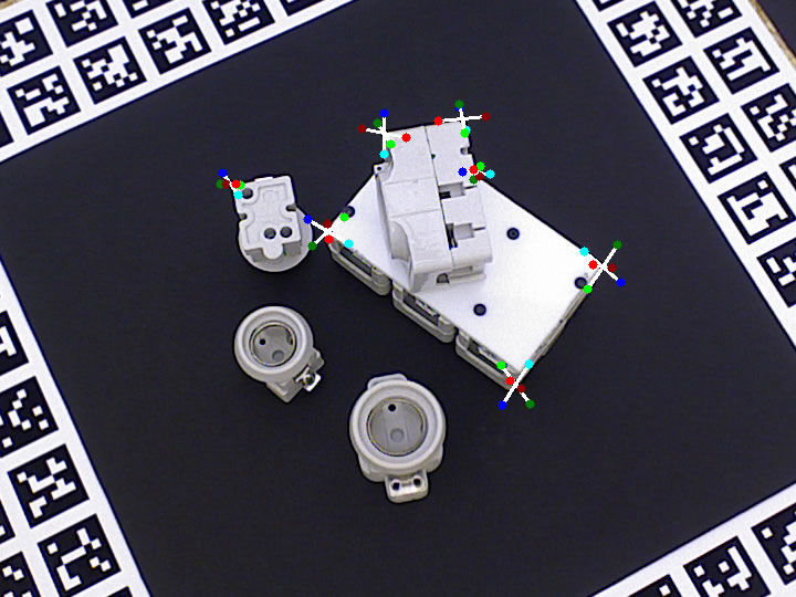
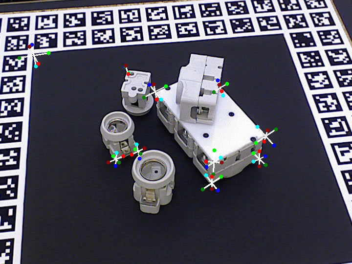
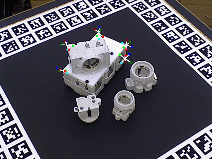
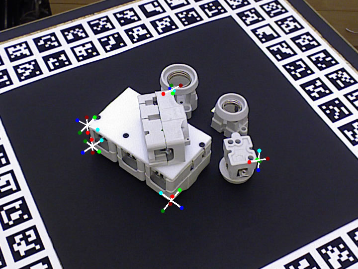
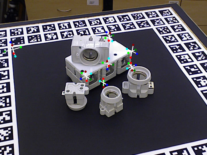
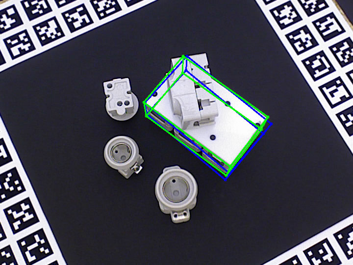
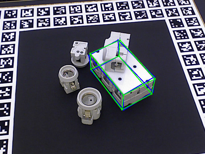
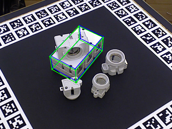
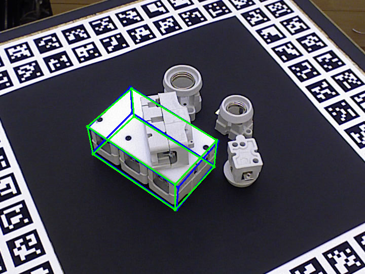
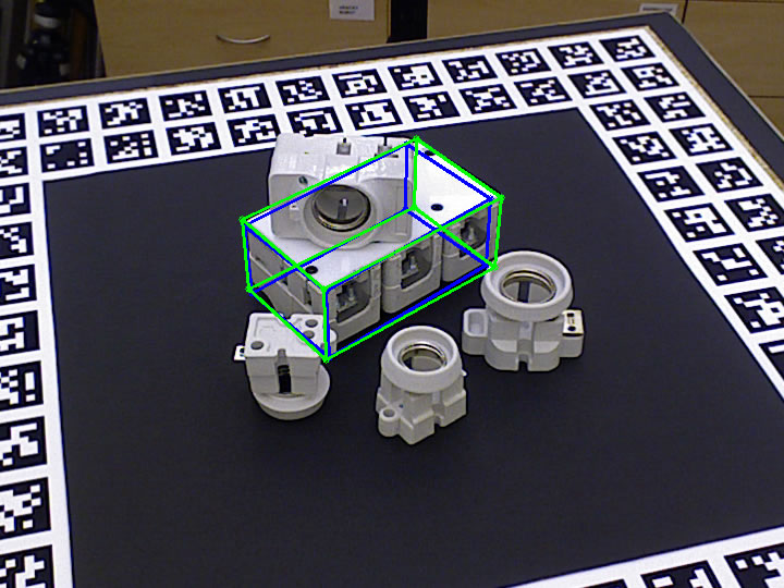
Figure 7: Some qualitative results on Object #7 in Scene #06 of the T-LESS dataset.

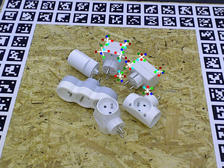
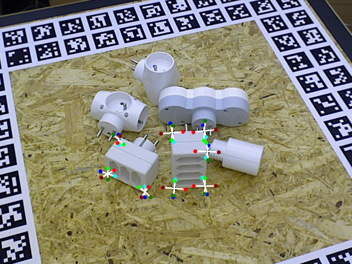
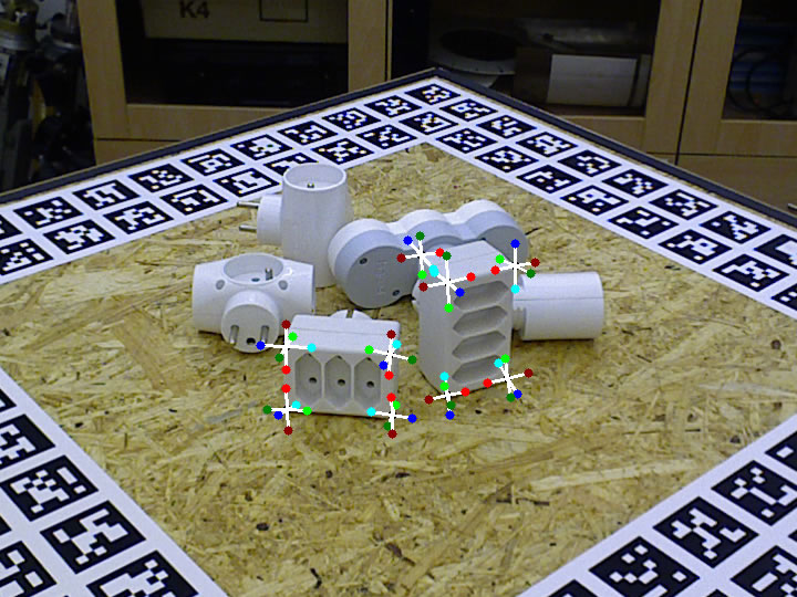
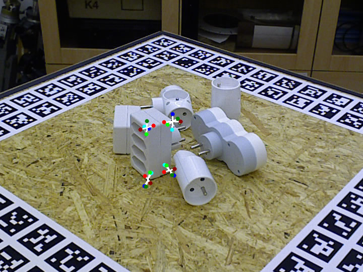
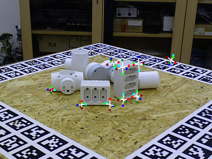
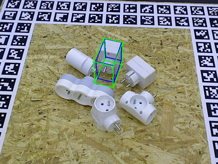
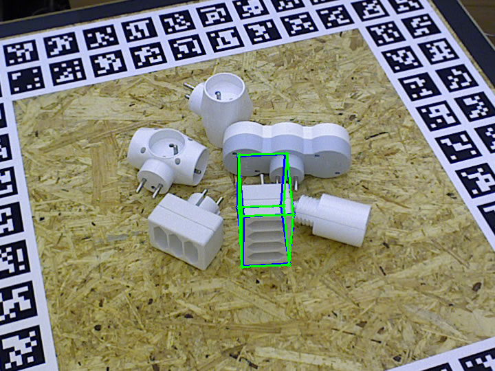
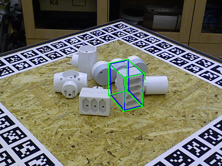
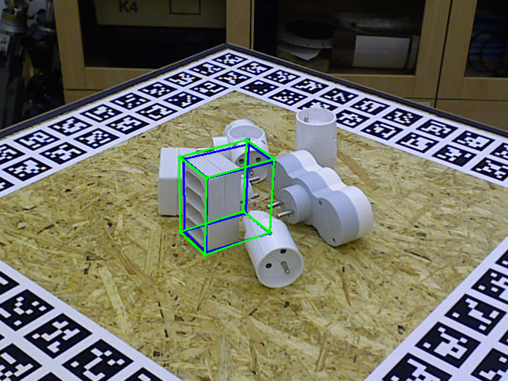
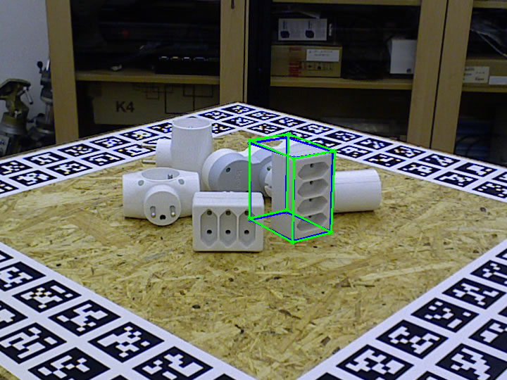
Figure 8: Some qualitative results on Object #20 in Scene #10 of the T-LESS dataset.

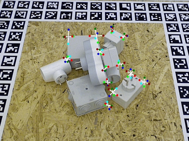
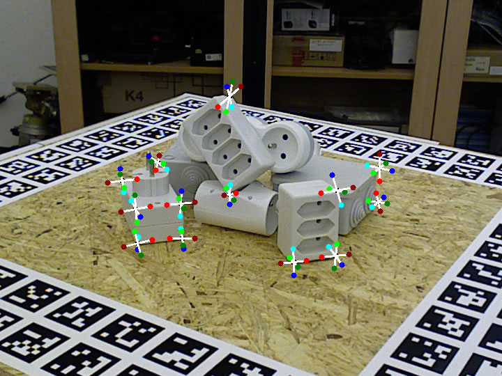
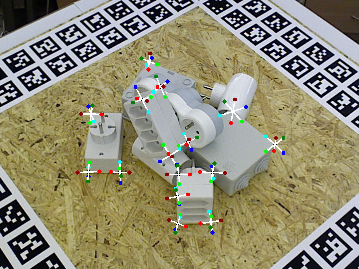
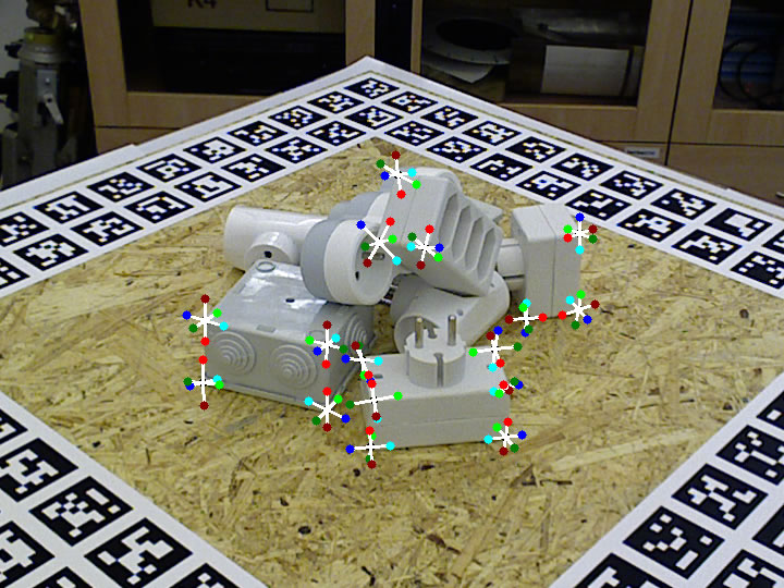
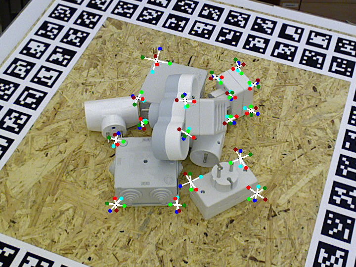
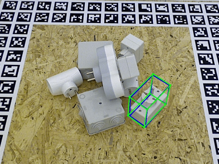
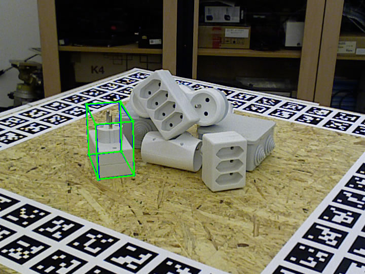
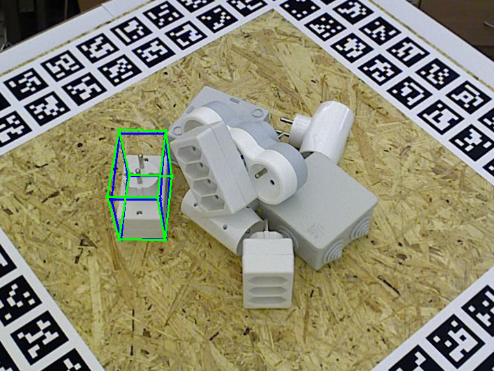
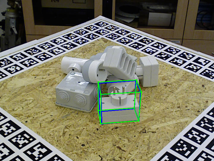
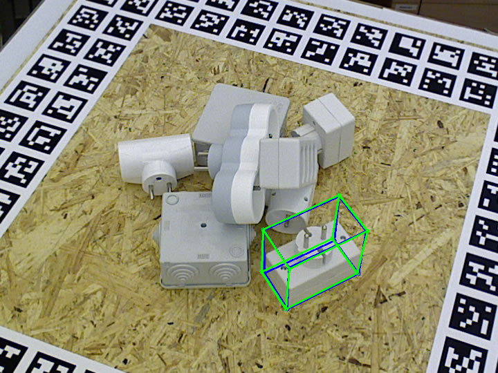
Figure 9: Some qualitative results on Object #20 in Scene #13 of the T-LESS dataset.

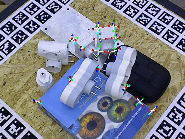
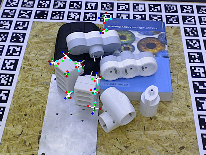
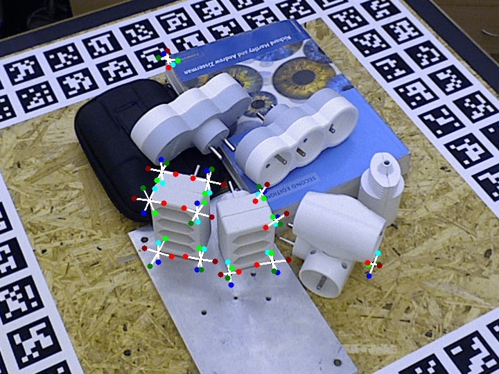
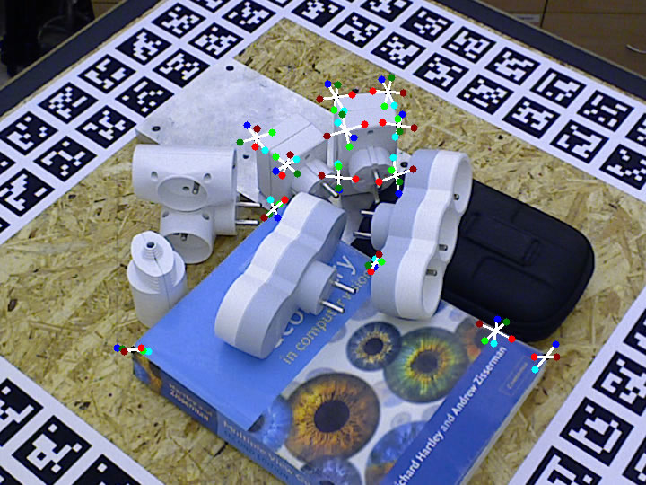
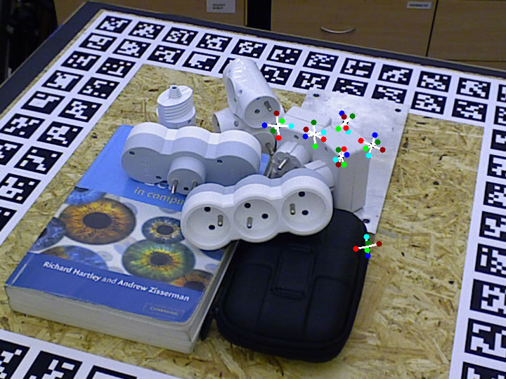
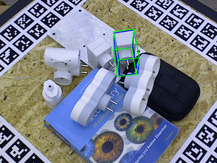
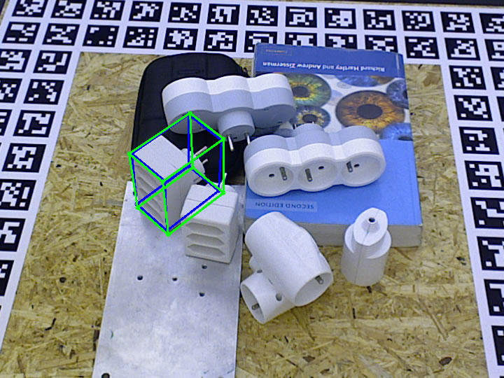
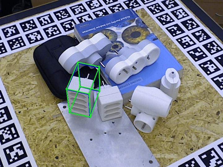
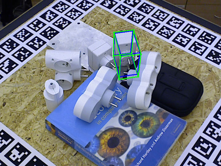
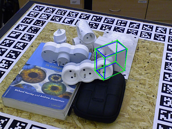
Figure 10: Some qualitative results on Object #20 in Scene #14 of the T-LESS dataset.

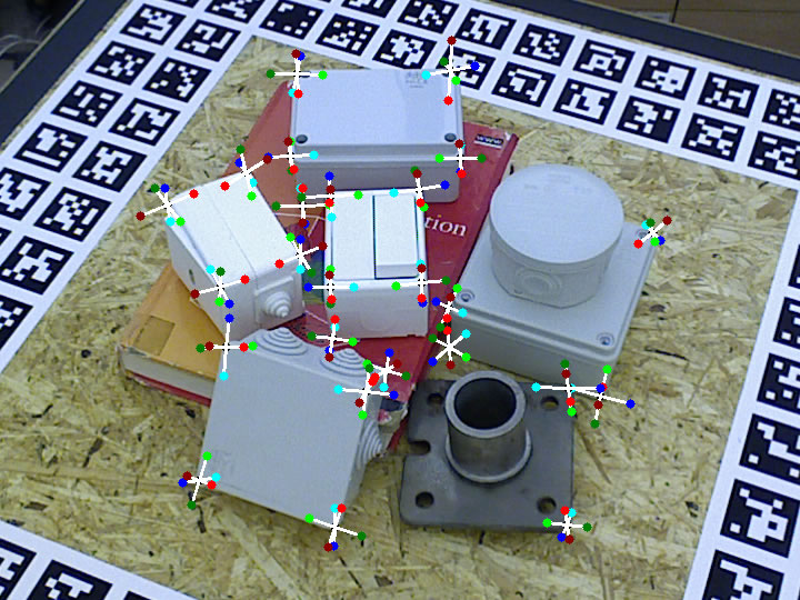
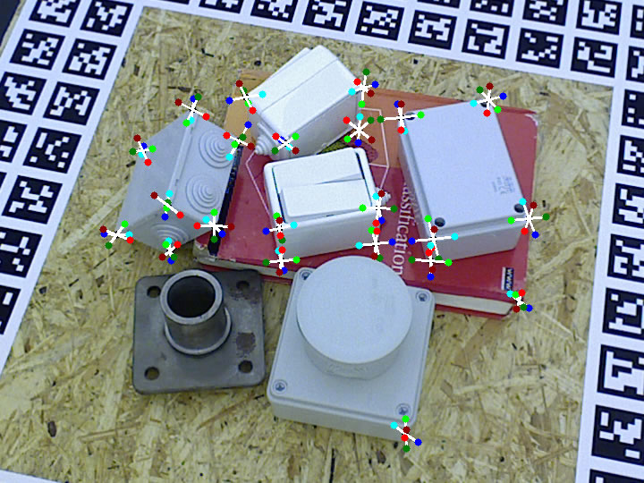
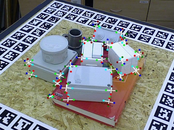
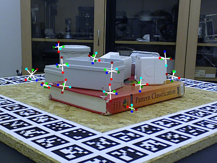
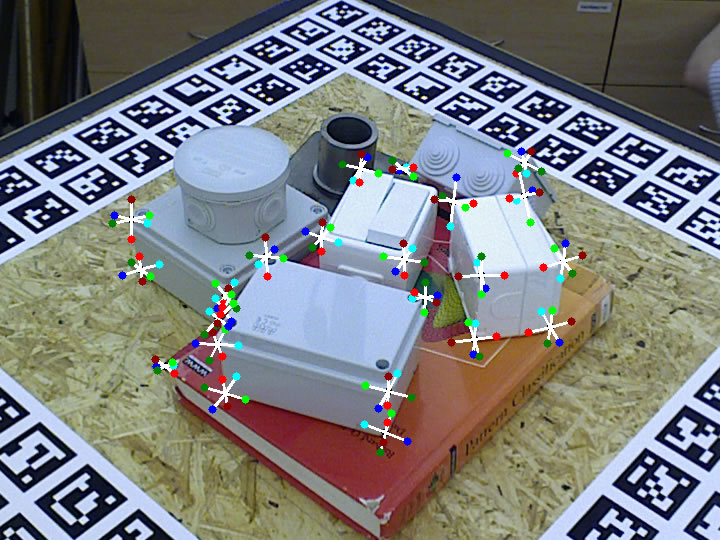
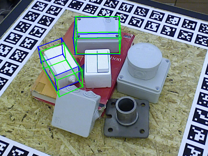
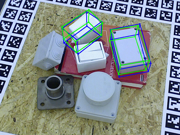
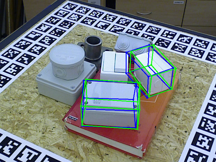
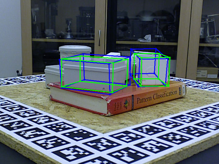
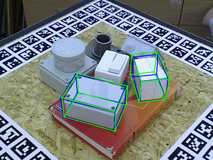
Figure 11: Some qualitative results on Object #26 and Object #29 in Scene #15 of the T-LESS dataset.

4.2.3 Qualitative results

To conclude the evaluation of our method, we present several qualitative results obtained on the tested scenes of the T-LESS dataset in Figs 6-11. Each top row show the results of the corners detection part while each bottom row shows the estimated 3D poses. Green boxes are ground truth 3D bounding boxes while blue boxes are bounding boxes we predicted using our pose estimation pipeline. Some scenes are very challenging. Here, the background is highly textured compared to the objects and the scenes are crowded with unwanted and close objects. Moreover, objects seen by our network during training appear near the objects on which we wanted to test our algorithm. Despite that, we can see that our method succeeds in estimating the pose correctly. Moreover, Figs. 7 and 10 show that detecting corners of the objects is a good direction when dealing with ”crowded” scenes where partial occlusions often occur.

4.3 Computation Times

We implemented our method on an Intel Xeon CPU E5-2609 v4 1.70GHz desktop with a GPU Quadro P5000. Our current implementation takes 300ms for the 3D part detection and 2s for the pose estimation, where most of the time is spent in rendering and cross-correlation. We believe this part could be significantly optimized.

5 Conclusion

We introduced a novel approach to the detection and 3D pose estimation of industrial objects in color images that only requires the CAD models of the objects, and no retraining is needed for new objects. We showed that estimating the 3D poses of the corners makes our method able to solve typical ambiguities that raise with industrial objects. A natural extension of our method would be to consider other types of parts, such as edges or quadric surfaces.

References

- [1] V. Balntas, A. Doumanoglou, C. Sahin, J. Sock, R. Kouskouridas, and T.-K. Kim. Pose Guided RGBD Feature Learning for 3D Object Pose Estimation. In International Conference on Computer Vision, 2017.
- [2] K. Bousmalis, N. Silberman, D. Dohan, D. Erhan, and D. Krishnan. Unsupervised Pixel-Level Domain Adaptation with Generative Adversarial Networks. In Conference on Computer Vision and Pattern Recognition, 2017.
- [3] K. Bousmalis, G. Trigeorgis, N. Silberman, D. Krishnan, and D. Erhan. Domain Separation Networks. In Advances in Neural Information Processing Systems, pages 343–351, 2016.
- [4] E. Brachmann, F. Michel, A. Krull, M. M. Yang, S. Gumhold, and C. Rother. Uncertainty-Driven 6D Pose Estimation of Objects and Scenes from a Single RGB Image. In Conference on Computer Vision and Pattern Recognition, 2016.
- [5] M. Bui, S. Zakharov, S. Albarqouni, S. Ilic, and N. Navab. When Regression Meets Manifold Learning for Object Recognition and Pose Estimation. In International Conference on Robotics and Automation, 2018.
- [6] G. Cai, Y. Wang, M. Zhou, and L. He. Unsupervised Domain Adaptation with Adversarial Residual Transform Networks. In arXiv Preprint, 2018.
- [7] A. Crivellaro, M. Rad, Y. Verdie, K. M. Yi, P. Fua, and V. Lepetit. Robust 3D Object Tracking from Monocular Images Using Stable Parts. IEEE Transactions on Pattern Analysis and Machine Intelligence, 2018.
- [8] T. Do, M. Cai, T. Pham, and I. Reid. Deep-6DPose: Recovering 6D Object Pose from a Single RGB Image. In arXiv Preprint, 2018.
- [9] B. Drost, M. Ulrich, N. Navab, and S. Ilic. Model Globally, Match Locally: Efficient and Robust 3D Object Recognition. In Conference on Computer Vision and Pattern Recognition, 2010.
- [10] Y. Ganin, E. Ustinova, H. Ajakan, P. Germain, H. Larochelle, F. Laviolette, M. Marchand, and V. Lempitsky. Domain-Adversarial Training of Neural Networks. Journal of Machine Learning Research, 2016.
- [11] I. J. Goodfellow, J. Pouget-Abadie, M. Mirza, B. Xu, D. Warde-Farley, S. Ozair, A. Courville, and Y. Bengio. Generative Adversarial Nets. In Advances in Neural Information Processing Systems, 2014.
- [12] S. Gupta, J. Hoffman, and J. Malik. Cross Modal Distillation for Supervision Transfer. In Conference on Computer Vision and Pattern Recognition, 2016.
- [13] R. Hartley and A. Zisserman. Multiple View Geometry in Computer Vision. Cambridge University Press, 2000.
- [14] K. He, G. Gkioxari, P. Dollar, and R. Girshick. Mask R-CNN. In International Conference on Computer Vision, 2017.
- [15] S. Hinterstoisser, C. Cagniart, S. Ilic, P. Sturm, N. Navab, P. Fua, and V. Lepetit. Gradient Response Maps for Real-Time Detection of Textureless Objects. IEEE Transactions on Pattern Analysis and Machine Intelligence, 2012.
- [16] S. Hinterstoisser, V. Lepetit, P. Wohlhart, and K. Konolige. On Pre-Trained Image Features and Synthetic Images for Deep Learning. In European Conference on Computer Vision Workshops, 2018.
- [17] T. Hodan, P. Haluza, S. Obdrzalek, J. Matas, M. Lourakis, and X. Zabulis. T-LESS: An RGB-D Dataset for 6D Pose Estimation of Texture-less Objects. In IEEE Winter Conference on Applications of Computer Vision, 2017.
- [18] O. H. Jafari, S. K. Mustikovela, K. Pertsch, E. Brachmann, and C. Rother. IPose: Instance-Aware 6D Pose Estimation of Partly Occluded Objects. CoRR, abs/1712.01924, 2017.
- [19] W. Kehl, F. Manhardt, F. Tombari, S. Ilic, and N. Navab. SSD-6D: Making RGB-Based 3D Detection and 6D Pose Estimation Great Again. In International Conference on Computer Vision, 2017.
- [20] H.-Y. Lee, H.-Y. Tseng, J.-B. Huang, M. Singh, and M.-H. Yang. Diverse Image-To-Image Translation via Disentangled Representations. In European Conference on Computer Vision, 2018.
- [21] W. Liu, D. Anguelov, D. Erhan, C. Szegedy, S. E. Reed, C.-Y. Fu, and A. C. Berg. SSD: Single Shot MultiBox Detector. In European Conference on Computer Vision, 2016.
- [22] M. Long, Y. Cao, J. Wang, and M. I. Jordan. Learning Transferable Features with Deep Adaptation Networks. In International Conference on Machine Learning, 2015.
- [23] F. Müller, F. Bernard, O. Sotnychenko, D. Mehta, S. Sridhar, D. Casas, and C. Theobalt. Ganerated Hands for Real-Time 3D Hand Tracking from Monocular RGB. In Conference on Computer Vision and Pattern Recognition, 2018.
- [24] S. Peng, Y. Liu, Q. Huang, H. Bao, and X. Zhou. Pvnet: Pixel-Wise Voting Network for 6DoF Pose Estimation. CoRR, abs/1812.11788, 2018.
- [25] M. Rad and V. Lepetit. BB8: A Scalable, Accurate, Robust to Partial Occlusion Method for Predicting the 3D Poses of Challenging Objects Without Using Depth. In International Conference on Computer Vision, 2017.
- [26] M. Rad, M. Oberweger, and V. Lepetit. Domain Transfer for 3D Pose Estimation from Color Images Without Manual Annotations. In Asian Conference on Computer Vision, 2018.
- [27] J. Redmon, S. Divvala, R. Girshick, and A. Farhadi. You Only Look Once: Unified, Real-Time Object Detection. In Conference on Computer Vision and Pattern Recognition, 2016.
- [28] S. Ren, K. He, R. Girshick, and J. Sun. Faster R-CNN: Towards Real-Time Object Detection with Region Proposal Networks. In Advances in Neural Information Processing Systems, 2015.
- [29] A. Rozantsev, M. Salzmann, and P. Fua. Beyond Sharing Weights for Deep Domain Adaptation. In Conference on Computer Vision and Pattern Recognition, 2017.
- [30] M. Sundermeyer, Z. Marton, M. Durner, M. Brucker, and R. Triebel. Implicit 3D Orientation Learning for 6D Object Detection from RGB Images. In European Conference on Computer Vision, 2018.
- [31] B. Tekin, S. N. Sinha, and P. Fua. Real-Time Seamless Single Shot 6D Object Pose Prediction. In Conference on Computer Vision and Pattern Recognition, 2018.
- [32] J. Tobin, R. Fong, A. Ray, J. Schneider, W. Zaremba, and P. Abbeel. Domain Randomization for Transferring Deep Neural Networks from Simulation to the Real World. In International Conference on Intelligent Robots and Systems, 2017.
- [33] E. Tzeng, J. Hoffman, T. Darrell, and K. Saenko. Simultaneous Deep Transfer Across Domains and Tasks. In International Conference on Computer Vision, 2015.
- [34] P. Wohlhart and V. Lepetit. Learning Descriptors for Object Recognition and 3D Pose Estimation. In Conference on Computer Vision and Pattern Recognition, 2015.
- [35] Y. Xiang, T. Schmidt, V. Narayanan, and D. Fox. PoseCNN: A Convolutional Neural Network for 6D Object Pose Estimation in Cluttered Scenes. Robotics: Science and Systems Conference, 2018.
- [36] S. Zakharov, W. Kehl, B. Planche, A. Hutter, and S. Ilic. 3D Object Instance Recognition and Pose Estimation Using Triplet Loss with Dynamic Margin. In International Conference on Intelligent Robots and Systems, 2017.
- [37] S. Zakharov, B. Planche, Z. Wu, A. Hutter, H. Kosch, and S. Ilic. Keep It Unreal: Bridging the Realism Gap for 2.5D Recognition with Geometry Priors Only. In International Conference on 3D Vision, 2018.
- [38] S. Zakharov, I. Shugurov, and S. Ilic. DPOD: Dense 6D Pose Object Detector and Refiner. In International Conference on Computer Vision, 2019.
- [39] J.-Y. Zhu, T. Park, P. Isola, and A. A. Efros. Unpaired Image-To-Image Translation Using Cycle-Consistent Adversarial Networks. In International Conference on Computer Vision, 2017.