Runge-Kutta and Networks

Abstract.

We categorify the RK family of numerical integration methods (explicit and implicit). Namely we prove that if a pair of ODEs are related by an affine map then the corresponding discrete time dynamical systems are also related by the map. We show that in practice this works well when the pairs of related ODEs come from the coupled cell networks formalism and, more generally, from fibrations of networks of manifolds.

In theory there is no difference between theory and practice. In practice, there is.

Attributed to various people

1. Introduction

The goal of the paper is to study the compatibility of the RK family of numerical integration methods with maps of dynamical systems. Our initial motivation was to understand why the fourth order explicit Runge-Kutta method (RK4) preserves polydiagonals in coupled cell networks even when these invariant subsystems (the polydiagonals) are exponentially unstable.

Coupled cell networks, which is an interesting class of continuous time dynamical systems, were introduced by Golubitsky, Stewart, Pivato and Török [4, 8]. They have been intensely studied by many mathematicians for a number of years. The polydiagonals of coupled cell networks are invariant subsystems that ultimately arise from the combinatorics of the networks in question. The framework of coupled cell networks has been generalized by the two of us [2, 3]. We showed that the combinatorics of the networks leads not only to invariant subsystems but more generally to maps between dynamical systems. Recall that maps between continuous time dynamical systems are maps between their phase spaces that send the trajectories of the first system to the trajectories of the second (see Definition 2.1 and subsequent remarks). Again we could see in examples that maps of continuous time dynamical systems were compatible with the discretizations provided by RK4.

The formalism of [3] has been generalized further to networks of open systems, see [6]. In particular, while the formalism [3] produces maps of dynamical systems that are essentially linear the formalism of [6] can produce pairs of dynamical systems related by truly nonlinear maps. The main theoretical result of the paper can be now formulated as follows. See Theorems 3.1 and 4.4 below for more precise formulations.

Theorem.  Let $X:\mathbb{R}^{n}\to\mathbb{R}^{n}$ and $Y:\mathbb{R}^{m}\to\mathbb{R}^{m}$ be a pair of maps defining the ODEs $\dot{x}=X(x)$ and $\dot{y}=Y(y)$. Let $L:\mathbb{R}^{n}\to\mathbb{R}^{m}$ be a linear map and $p\in\mathbb{R}^{m}$ a vector. Suppose

$$Y(Lx+p)=L(X(x))$$

for all $x\in\mathbb{R}^{n}$. Let $D_{X}:\mathbb{R}^{n}\to\mathbb{R}^{n}$, $D_{Y}:\mathbb{R}^{m}\to\mathbb{R}^{m}$ denote a pair of discrete time dynamical system produced by a Runge-Kutta method (explicit or implicit). Then

$$D_{y}Y\,(Lx+p)=L(D_{X}(x))+p$$

for all $x\in\mathbb{R}^{n}$.

Equivalently, if a map of dynamical systems $f:(X,\mathbb{R}^{n})\to(Y,\mathbb{R}^{m})$ is affine (i.e., $f(x)=Lx+p$ for some linear map $L:\mathbb{R}^{n}\to\mathbb{R}^{m}$) then $f$ sends a trajectory $\{x_{n}=(D_{X})^{n}(x_{0})\}_{n=1}^{\infty}$ of the discretized system $D_{X}$ to the trajectory $\{y_{n}=(D_{Y})^{n}(f(x_{0}))\}_{n=1}^{\infty}$ of the discretized system $D_{Y}$.

In the case of coupled cell networks $\mathbb{R}^{n}=\mathbb{R}^{n_{1}}\times\mathbb{R}^{n_{2}}\times\cdots\times\mathbb{R}^{n_{r}}$, $\mathbb{R}^{m}=(\mathbb{R}^{n_{1}})^{k_{1}}\times(\mathbb{R}^{n_{2}})^{k_{2}}\times\cdots\times(\mathbb{R}^{n_{r}})^{k_{r}}$ for some $n_{1},\ldots,n_{r}$, $k_{1},\ldots,k_{r}$ and the map

$$f:\mathbb{R}^{n_{1}}\times\mathbb{R}^{n_{2}}\times\cdots\times\mathbb{R}^{n_{r}}\to(\mathbb{R}^{n_{1}})^{k_{1}}\times(\mathbb{R}^{n_{2}})^{k_{2}}\times\cdots\times(\mathbb{R}^{n_{r}})^{k_{r}}$$

is of the form

$$f(x_{1},\ldots x_{r})=(\underbrace{(x_{1},\ldots,x_{1})}_{k_{1}},\ldots,\underbrace{(x_{r},\ldots,x_{r})}_{k_{r}}).$$

Thus our theorem proves that polydiagonals in coupled cell networks are preserved by any numerical method in the RK family. We give an example to show that this works in practice even if the polydiagonal (that is, the invariant subsystem $f(\mathbb{R}^{n})$) is exponentially unstable. We admit that at the first glance this may seem “obvious” for explicit methods given the form of the map $f$. After all, $f$ is just duplicating certain groups of coordinates. We hope that upon further reflection the reader will see that this is not completely obvious even in the case of explicity methods. Recall that an explict RK method require composing two or more nonlinear maps, taking a linear combinations of the composites, composing again and so on. It requires an argument why a repeated application of these operations preserves duplication of coordinates.

Organization of the paper

In section 2 we recall some of the relevant background material. In section 3 we prove our main theorem for explict RK methods. In section 4 we extend the result to implicit RK methods. Section 5 is taken up with examples. There we show that explicity fourth order Runge-Kutta (RK4) works well for preserving polydiagonals and affine polydiagonals. We then illustrate a difference between theory and practice by an example of a linear map of dynamical systems that in practice does not preserve the discretizations. The issue is likely to be the roundoff errors. Finally we give an example of an invariant parabola in $\mathbb{R}^{2}$ which is not preserved by RK4. We agree that this should not be surprising since non-geometric numerical methods are not known for their ability to preserve nonlinear invariant submanifolds.

2. Background

We start with the key definition, which is standard in differential geometry.

Definition 2.1.

Let $f:N\to M$ be a differentiable map between two manifolds. A vector field $X$ on $N$ is $f$-related to the vector field $Y$ on $M$ if

(2.2) $$df_{x}(X(x))=Y(f(x))$$

for all $x\in N$. Here and elsewhere $df_{x}:T_{x}N\to T_{f(x)}M$ denotes the differential of the map $f$.

Remark 2.3.

In the case where $N=\mathbb{R}^{n}$ and $M=\mathbb{R}^{m}$ the vector field $X$ on $N$ is usually identified with a map $X:\mathbb{R}^{n}\to\mathbb{R}^{n}$, and similarly $Y$ is identified with a map $Y:\mathbb{R}^{m}\to\mathbb{R}^{m}$. The equation (2.2) then reduces to

$$df(x)\,X(x)=Y(f(x))$$

where $df(x)$ is the Jacobian matrix of the map $f$.

Remark 2.4.

A simple application of the uniqueness of solutions of ODEs and of the chain rule shows that if a vector field $X$ on a manifold $N$ is $f:N\to M$ related to a vector field $Y$ on a manifold $M$ then for any integral curve $\gamma(t)$ of $X$, $f(\gamma(t))$ is an integral curve of $Y$. See for example [10].

Remark 2.5.

It is common to refer to a pair $(N,X)$ where $N$ is a manifold and $X$ is a vector field on $N$ as a continuous time dynamical system. A map of dynamical systems from a system $(N,X)$ to a system $(M,Y)$ is a differntiable map $f:N\to M$ so that $X$ is $f$-related to $Y$. Continuous time dynamical systems and their maps form a category, see for example [6]. One may may interpret the main results of the paper as an attempt to construct a class of functors from a category of continuous time systems to the category of discrete time systems using numerical integration methods. The attempt succeeds in the case where the objects of the source category are Euclidean (i.e., coordinate) vector spaces, the morphisms are affine maps and the functors are constructed using the RK integration methods.

We now turn to numerical methods.

Definition 2.6.

Consider a vector field $X:\mathbb{R}^{n}\to\mathbb{R}^{n}$. Choose $s\in\mathbb{N}$, $\{a_{ij}\}_{i,j=1}^{s}$, and $\{b_{i}\}_{i=1}^{s}$. The Runge-Kutta method with matrix $a_{ij}$, weights $b_{i}$, and stepsize $h$, denoted $D_{X}^{(A,b,h)}$, is defined as follows (see  [9, (12.51), pages 351—352]): For $i=1,\dots,s$, we set

$$k_{X,i}(x):=X\left(x+h\sum_{j=1}^{s}a_{i,j}k_{X,j}(x)\right),$$

and then

$$D_{X}^{(A,b,h)}(x):=x+h\sum_{i=1}^{s}b_{i}k_{X,i}(x).$$

We say that the method is explicit if $a_{ij}=0$ whenever $i\leq j$. Otherwise the method is implicit.

Remark 2.7.

In an explicit RK method for a vector field $X$

$$k_{X,1}(x) := X(x),$$

$$k_{X,2}(x) := X(x+ha_{2,1}k_{X,1}(x)),$$

$$k_{X,3}(x) := X(x+h(a_{3,1}k_{X,1}(x))+a_{3,2}k_{X,2}(x)))),$$

$$\vdots$$

$$k_{X,i}(x) := X(x+h(a_{i,1}k_{X,1}(x)+\cdots+a_{i,i-1}k_{X,i-1}(x)))$$

$$\vdots$$

Once a Runge-Kutta method is fixed, we numerically integrate the ODE

(2.8) $$\dot{x}=X(x),x(0)=x_{0}$$

by the following iterative scheme:

$$x_{n+1}=D_{X}^{(A,b,h)}(x_{n}),\qquad\textrm{ for all }n\geq 0.$$

There is a large theory of the accuracy, efficiency, convergence, and consistency of such methods, which we do not address here. See, for example, [9, 5]. Under certain well-understood conditions, the solution (integral curve) $x(t)$ of (2.8) will be well-approximated by $x_{\lfloor(t/h)\rfloor}$ for all $t\geq 0$.

Example 2.1.

The fourth order Runge-Kutta method (RK4) is defined by the following data:

$$A=\left(\begin{array}[]{cccc}0&0&0&0\\ 1/2&0&0&0\\ 0&1/2&0&0\\ 0&0&1&0\end{array}\right),\quad b=(1/6,1/3,1/3,1/6)^{T}.$$

Note that RK4 is explicit.

3. Explicit RK methods

In this section we prove

Theorem 3.1.

Let $X:\mathbb{R}^{n}\to\mathbb{R}^{n}$ and $Y:\mathbb{R}^{m}\to\mathbb{R}^{m}$ be two vector fields, $L:\mathbb{R}^{n}\to\mathbb{R}^{m}$ a linear map and $p\in\mathbb{R}^{m}$, such that

(3.2) $$LX(x)=Y(Lx+p)\qquad\textrm{ for all }x\in\mathbb{R}^{n}.$$

Then for any choice of a vector $b$ and a matrix $(a_{i,j})$ in Definition 2.6 that gives an explicit RK method (i.e., $a_{ij}=0$ for $i\leq j$), we have

(3.3) $$LD_{X}^{(A,b,h)}(x)+p=D_{Y}^{(A,b,h)}(Lx+p).$$

Remark 3.4.

Let $X$, $Y$, $f(x)=Lx+p$, $D_{X}^{(A,b,h)}$ and $D_{Y}^{(A,b,h)}$ be as above. Pick $x_{0}\in\mathbb{R}^{n}$. Set $y_{0}:=f(x_{0})=Lx_{0}+p$. Define recursively

$$x_{n+1}:=DX^{(A,b,h)}(x_{n})\qquad\textrm{and}\qquad y_{n+1}:=DY^{(A,b,h)}(y_{n}).$$

An induction argument based on Theorem 3.1 implies that

$$y_{n}=f(x_{n})$$

for all $n$.

Our proof of Theorem 3.1 is based on a lemma.

Lemma 3.5.

Fix $q\geq 0$. Let $f:\mathbb{R}^{n}\to\mathbb{R}^{m}$, $f(x)=Lx+p$ be an affine map as in Theorem 3.1. Let $f_{0},f_{1},\dots,f_{q}:\mathbb{R}^{n}\to\mathbb{R}^{n}$ and $g_{0},g_{1},\dots,g_{q}:\mathbb{R}^{m}\to\mathbb{R}^{m}$ be two collections of maps where

$$g_{k}(Lx+p)=Lf_{k}(x)\qquad\textrm{for all }0\leq k\leq q.$$

Fix $\gamma_{1},\dots,\gamma_{q}\in\mathbb{R}$ and define the functions $\varphi:\mathbb{R}^{n}\to\mathbb{R}^{n}$ and $\psi:\mathbb{R}^{m}\to\mathbb{R}^{m}$ by

$$\varphi(x) :=f_{0}\left(x+\sum_{i=1}^{q}\gamma_{i}f_{i}(x)\right),$$

$$\psi(y) :=g_{0}\left(y+\sum_{i=1}^{q}\gamma_{i}g_{i}(y)\right).$$

Then

$$\psi(Lx+p)=L\varphi(x).$$

Proof.

The proof is a computation:

$$\psi(Lx+p) =g_{0}\left(Lx+p+\sum_{i=1}^{q}\gamma_{i}g_{i}(Lx+p)\right)$$

$$=g_{0}\left(Lx+p+\sum_{i=1}^{q}\gamma_{i}Lf_{i}(x)\right)$$

$$=g_{0}\left(L\left(x+\sum_{i=1}^{q}\gamma_{i}f_{i}(x)\right)+p\right)$$

$$=Lf_{0}\left(x+\sum_{i=1}^{q}\gamma_{i}f_{i}(x)\right)=L\varphi(x).$$

∎

Proof of Theorem 3.1.

We first prove by induction that

(3.6) $$k_{Y,i}(Lx+p)=Lk_{X,i}(x)$$

for all $i=1,\dots,s$. Since $k_{X,1}(x)=X(x)$ and $k_{Y,1}(x)=Y(x)$, the equation (3.6) holds for $i=1$ by assumption: see (3.2). Now assume that (3.6) holds for $j=1,\dots,i-1$. Then we compute:

$$k_{Y,i}(Lx+p) =Y\left((Lx+p)+h\sum_{j=1}^{i-1}a_{i,j}k_{Y,j}(Lx+p)\right)$$

$$=Y\left(Lx+p+h\sum_{j=1}^{i-1}a_{i,j}L\big{(}k_{X,j}(x)\big{)}\right)$$ by inductive assumption

$$=Y\left(L\left(x+h\sum_{j=1}^{i-1}a_{i,j}k_{X,j}(x)\right)+p\right)$$ by Lemma 3.5

$$=LX\left(x+h\sum_{j=1}^{i-1}a_{i,j}k_{X,j}(x)\right) =Lk_{X,i}(x).$$

Finally

$$D_{Y}^{(A,b,h)}(Lx+p) =(Lx+p)+h\sum_{j=1}^{s}b_{j}k_{Y,j}(Lx+p)=(Lx+p)+h\sum_{j=1}^{s}b_{j}L\big{(}k_{X,j}(x)\big{)}$$

$$=L\left(x+h\sum_{j=1}^{s}b_{j}k_{X,j}(x)\right)+p=LD_{X}^{(A,b)}(x)+p,$$

and we are done. ∎

4. Implicit RK methods

We now consider implicit Runge–Kutta methods. Recall the defining equation for the functions $k_{X,i}$ in Definition 2.6:

(4.1) $$k_{X,i}(x)=X\left(x+h\sum_{j=1}^{s}a_{i,j}k_{X,j}(x)\right).$$

Unless the numbers $a_{i,j}=0$ for all $i\leq j$ (3.6) is a system of nonlinear “algebraic” equations. In general there no easy way to solve this system of equations and obtain a formula for $k_{X,i}(x)$ in terms of $k_{X,1}$, …, $k_{X,i-1}$. One solution to the problem is to choose a small enough step $h$ so that the contraction mapping principle applies to the appropriately defined map. Then one chooses a starting point and iterates. See for example [5, Chapter 6].

Definition 4.2.

We define an implicit Runge-Kutta method with $q$-step iterative solution as follows: Choose $s,A,b,h$ as in Definition 2.6. Choose a positive integer $q$ and fix a point $x\in\mathbb{R}^{n}$. Define a map

$$\underline{X}:(\mathbb{R}^{n})^{s}\to(\mathbb{R}^{n})^{s}$$

by

(4.3) $$\underline{X}(\xi_{1},\ldots,\xi_{s})=\left(X\left(x+h\sum_{j=1}^{s}a_{1,j}\xi_{j}\right),\ldots,X\left(x+h\sum_{j=1}^{s}a_{s,j}\xi_{j}\right)\right)$$

for all $\boldsymbol{\xi}=(\xi_{1},\ldots,\xi_{s})\in(\mathbb{R}^{n})^{s}$.Choose $\boldsymbol{\xi}^{(0)}=(X(x),\ldots,X(x))$. Define $\boldsymbol{\xi}^{(k+1)}\in(\mathbb{R}^{n})^{s}$ recursively by $\boldsymbol{\xi}^{(k+1)}:=\underline{X}(\boldsymbol{\xi}^{(k)})$ for $k=0,\ldots,q-1$. Now define

$$D_{X}^{(A,b,h,q)}(x):=x+h\sum_{i=1}^{s}b_{i}\xi_{i}^{(q)}.$$

We are now in position to state the second main result of the paper.

Theorem 4.4.

Let $L:\mathbb{R}^{n}\to\mathbb{R}^{m}$ a linear map, $p\in\mathbb{R}^{m}$ a point and let $X:\mathbb{R}^{n}\to\mathbb{R}^{n}$ and $Y:\mathbb{R}^{m}\to\mathbb{R}^{m}$ be two vector fields such that

(3.2) $$LX(x)=Y(Lx+p)\qquad\textrm{ for all }x\in\mathbb{R}^{n}.$$

Define $D_{X}^{(A,b,h,q)}(x)$, $D_{Y}^{(A,b,h,q)}(y)$ as above in Definition 4.2. Then for any choice of the parameters $A,b,h$ and $q$ and for any $x\in\mathbb{R}^{n}$

(3.3) $$LD_{X}^{(A,b,h,q)}(x)+p=D_{Y}^{(A,b,h,q)}(Lx+p).$$

Proof.

By definition $D_{X}^{(A,b,h,q)}(x):=x+h\sum_{i=1}^{s}b_{i}\xi_{i}^{(q)}$ where $\boldsymbol{\xi}^{(q)}$ is defined recursively by

$$\boldsymbol{\xi}^{(0)}=(X(x),\ldots,X(x))\qquad\textrm{and}\qquad\boldsymbol{\xi}^{(k+1)}:=\underline{X}(\boldsymbol{\xi}^{(k)})\textrm{ for }k=0,\ldots,q-1;$$

and $\underline{X}:(\mathbb{R}^{n})^{s}\to(\mathbb{R}^{n})^{s}$ is given by (4.3). Define $\underline{Y}:(\mathbb{R}^{m})^{s}\to(\mathbb{R}^{n})^{s}$ by changing what needs to be changed in (4.3). In particular $x$ is replaced by $Lx+p$. Let

$$\boldsymbol{\eta}^{(0)}=(Y(Lx+p),\ldots,Y(Lx+p))=(\overbrace{L\times\cdots\times L}^{s})\,(\boldsymbol{\xi}^{(0)})\in(\mathbb{R}^{m})^{s}$$

and define $\boldsymbol{\eta}^{(q)}$ recursively by

$$\boldsymbol{\eta}^{(k+1)}:=\underline{Y}(\boldsymbol{\eta}^{(k)})\quad\textrm{ for }k=0,\ldots,q-1.$$

It is easy to show by induction that

$$\boldsymbol{\eta}^{(k)}=(\overbrace{L\times\cdots\times L}^{s})\,(\boldsymbol{\xi}^{(k)})$$

for $k=1,\ldots,q$. Here is a proof of the inductive step:

$$\boldsymbol{\eta}^{(k+1)} =\left(Y\left(y+h\sum_{j=1}^{s}a_{1,j}\eta^{(k)}_{j}\right),\ldots,Y\left(y+h\sum_{j=1}^{s}a_{s,j}\eta^{(k)}_{j}\right)\right)$$

$$=\left(Y\left(Lx+p+h\sum_{j=1}^{s}a_{1,j}L\xi^{(k)}_{j}\right),\ldots,Y\left(Lx+p+h\sum_{j=1}^{s}a_{s,j}L\xi^{(k)}_{j}\right)\right)$$

$$=\left(Y\left(L\left(x+h\sum_{j=1}^{s}a_{1,j}\xi^{(k)}_{j}\right)+p\right),\ldots,Y\left(L\left(x+h\sum_{j=1}^{s}a_{s,j}\xi^{(k)}_{j}\right)+p\right)\right)$$

$$=\left(LX\left(x+h\sum_{j=1}^{s}a_{1,j}\xi^{(k)}_{j}\right),\ldots,Lx\left(L(x+h\sum_{j=1}^{s}a_{s,j}\xi^{(k)}_{j}\right)\right)$$

$$=\left(L\xi^{(k+1)}_{1},\ldots,L\xi^{(k+1)}_{s}\right)=(\overbrace{L\times\cdots\times L}^{s})\,(\boldsymbol{\xi}^{(k+1)}).$$

In particular

$$\left(\eta^{(q)}_{1},\ldots,\eta^{(q)}_{s}\right)=\left(L\xi^{(q)}_{1},\ldots,L\xi^{(q)}_{s}\right).$$

Finally

$$D_{Y}^{(A,b,h,q)}(Lx+p) =(Lx+p)+h\sum_{i=1}^{s}b_{i}\eta_{i}^{(q)}=(Lx+p)+h\sum_{i=1}^{s}b_{i}L\xi_{i}^{(q)}$$

$$=L\left(x+h\sum_{i=1}^{s}b_{i}\xi_{i}^{(q)}\right)+p=LD_{X}^{(A,b,h,q)}(x)+p.$$

∎

5. Examples

We present several examples illustrating the results of the theorems above. In many of the examples listed below, we want to check whether or not the vector fields are related in the sense defined in the introduction. As such, one of the quantities that we plot is the scalar quantity $\left\|{D_{Y}\circ f-f\circ D_{X}}\right\|_{1}$, where the subscript denotes that we are taking the $\ell^{1}$ norm of the vector. This quantity is identically zero if the vector fields $X$ and $Y$ are $f$-related.

Example 5.1.

Consider the vector field

(5.1) $$Y:\mathbb{R}^{2}\to\mathbb{R}^{2},\qquad Y\begin{pmatrix}x_{1}\\ x_{2}\end{pmatrix}=\begin{pmatrix}-x_{1}-2x_{2}+(x_{1}-x_{2})x_{1}^{3}\\ -2x_{1}-x_{2}\end{pmatrix}.$$

It is easy to see that $\Delta=\{x_{1}=x_{2}\}$ is an invariant submanifold of the vector field $Y$, since $Y\begin{pmatrix}x\\ x\end{pmatrix}=-3\begin{pmatrix}x\\ x\end{pmatrix}$. The linearization of $Y$ at the origin (in fact, along any point on the diagonal $\{x_{1}=x_{2}\}$) is the matrix $\begin{pmatrix}-1&-2\\ -2&-1\end{pmatrix}$. It follows that the diagonal $\Delta$ is an unstable submanifold of $Y$. Nonetheless, the diagonal is preserved by numerical integration.

Now for any vector field $Y$ on a manifold $M$ and an invariant submanifold $\Sigma$ of $Y$ the inclusion $f:\Sigma\hookrightarrow M$ relates the restriction $X=Y|_{\Sigma}$ and $Y$. In the case of the example before us, the inclusion $L:\Delta\to\mathbb{R}^{2}$ of the invariant submanifold is $L(u)=(u,u)$ and $X(u)=-3u$. Since the map $L$ is linear Theorem 3.1 applies. Figure 1 graphically illustrates Theorem 3.1 for this pair of systems: it shows that $LD_{X}^{(A,b,h)}(x)=D_{Y}^{(A,b,h)}(Lx)$, which by extension demonstrates the invariance of the diagonal. The left figure shows a phase portrait of system 5.1 while the right figure shows agreement of numerical integration.

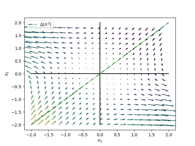
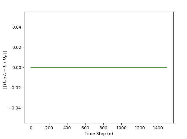
Figure 1. Numerics for system (5.1). The left figure shows a phase portrait of system 5.1 while the right figure shows agreement of numerical integration.

Example 5.2.

This example shows that affine invariant submanifolds also are preserved in practice. We consider the vector field

(5.2) $$Y:\mathbb{R}^{2}\to\mathbb{R}^{2},\qquad Y\begin{pmatrix}x_{1}\\ x_{2}\end{pmatrix}=\begin{pmatrix}-x_{1}-2x_{2}+1\\ -2x_{1}-x_{2}\end{pmatrix}.$$

The map

$$f:\mathbb{R}\to\mathbb{R}^{2},\qquad f(u)=(u,u+1)$$

is of the form $f(u)=Lu+(0,1)$ where $L:\mathbb{R}\to\mathbb{R}^{2}$ is the linear map $L(u)=(u,u)$. The affine map $f$ relates the vector field $X(u)=-3u-1$ and $Y$:

$$Y(f(u))=Y(u,u+1)=(-3u-1,-3u-1)=Df(u)\,\,X(u).$$

Thus the affine submanifold $\{x_{2}=x_{1}+1\}$ is an invariant submanifold of $X$. A simulation shows that Runge-Kutta preserves this “offset” diagonal.

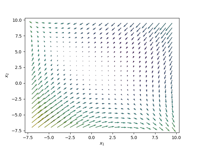
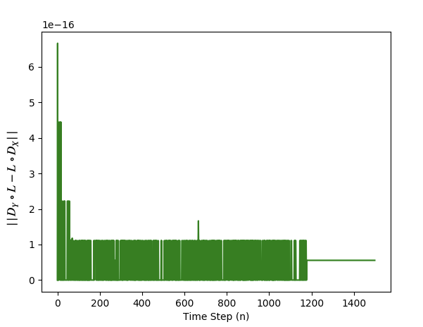
Figure 2. Numerics for system 5.2. The left figure shows a phase portrait of system 5.1 while the right figure shows agreement of numerical integration.

Example 5.3.

In this example we consider a pair of related vector fields produced by the networks of manifolds formalism of [3]. Suppose we choose any three functions $w_{1}:\mathbb{R}\to\mathbb{R}$, $w_{2}:\mathbb{R}^{3}\to\mathbb{R}$ and $w_{3}:\mathbb{R}^{2}\to\mathbb{R}$. Define a vector field $X:\mathbb{R}^{3}\to\mathbb{R}^{3}$ by

$$X(x_{1},x_{2},x_{3})=(w_{1}(x_{1}),w_{2}(x_{2},x_{1},x_{1}),w_{3}(x_{3},x_{2})).$$

Define a vector field $Y:\mathbb{R}^{3}\to\mathbb{R}^{3}$ by

$$Y(y_{1},y_{2},y_{3})=(w_{1}(y_{1}),w_{1}(y_{2}),w_{2}(y_{3},y_{1},y_{2})).$$

The first vector field comes from the network

(5.3)

and the second from the network

(5.4) $$\lx@xy@svg{\hbox{\raise 0.0pt\hbox{\kern 35.39702pt\hbox{{\hbox{\kern-35.39702pt\raise 0.0pt\hbox{\hbox{\kern 0.0pt\raise-3.22223pt\hbox{$\textstyle{1\,\bullet}$}}}}}{\hbox{\kern 25.9526pt\raise 0.0pt\hbox{\hbox{\kern 0.0pt\raise-2.22223pt\hbox{$\textstyle{\bullet}$}}}}}{\hbox{\kern 22.9526pt\raise 8.53578pt\hbox{\hbox{\kern 3.0pt\raise-3.22223pt\hbox{$\textstyle{2}$}}}}}{\hbox{\kern 78.4134pt\raise 0.0pt\hbox{\hbox{\kern 0.0pt\raise-3.22223pt\hbox{$\textstyle{\bullet\,3}$}}}}}\ignorespaces\ignorespaces\ignorespaces\ignorespaces\ignorespaces\ignorespaces\ignorespaces\ignorespaces\ignorespaces{}{}{}{{}{}{}{}{}{}{}{}{}{}{}{}}{}\ignorespaces\ignorespaces\hbox{\hbox{\kern 0.0pt\raise 0.0pt\hbox{{}{}{{}}{{}{}{}}{}}}}\ignorespaces{}\ignorespaces{}{}{}{{}{}{}{}{}{}{}{}{}{}{}{}{}{}{}{}{}}{\hbox{\kern 25.95193pt\raise 2.01668pt\hbox{\hbox{\kern 0.0pt\raise 0.0pt\hbox{\lx@xy@tip{1}\lx@xy@tip{-1}}}}}}\ignorespaces\ignorespaces\hbox{\hbox{\kern 0.0pt\raise 0.0pt\hbox{{}{}{}{{}}{{}{}{}\lx@xy@spline@}{}}}}\ignorespaces{}\ignorespaces\hbox{\hbox{\kern 0.0pt\raise 0.0pt\hbox{{}{}{{}}{{}{}{}}{}}}}\ignorespaces{}\ignorespaces\ignorespaces\ignorespaces\ignorespaces\ignorespaces\ignorespaces\ignorespaces\ignorespaces\ignorespaces\ignorespaces{}{}{}{{}{}{}{}{}{}{}{}{}{}{}{}}{}\ignorespaces\ignorespaces\hbox{\hbox{\kern 0.0pt\raise 0.0pt\hbox{{}{}{{}}{{}{}{}}{}}}}\ignorespaces{}\ignorespaces{}{}{}{{}{}{}{}{}{}{}{}{}{}{}{}{}{}{}{}{}}{\hbox{\kern 25.95193pt\raise-2.01668pt\hbox{\hbox{\kern 0.0pt\raise 0.0pt\hbox{\lx@xy@tip{1}\lx@xy@tip{-1}}}}}}\ignorespaces\ignorespaces\hbox{\hbox{\kern 0.0pt\raise 0.0pt\hbox{{}{}{}{{}}{{}{}{}\lx@xy@spline@}{}}}}\ignorespaces{}\ignorespaces\hbox{\hbox{\kern 0.0pt\raise 0.0pt\hbox{{}{}{{}}{{}{}{}}{}}}}\ignorespaces{}\ignorespaces\ignorespaces\ignorespaces\ignorespaces\ignorespaces\ignorespaces\ignorespaces\ignorespaces{}\ignorespaces{\hbox{\lx@xy@droprule}}\ignorespaces{\hbox{\kern 78.4134pt\raise 0.0pt\hbox{\hbox{\kern 0.0pt\raise 0.0pt\hbox{\lx@xy@tip{1}\lx@xy@tip{-1}}}}}}\ignorespaces{\hbox{\lx@xy@droprule}}{\hbox{\lx@xy@droprule}}\ignorespaces}}}}\quad. \textstyle{1\,\bullet} \textstyle{\bullet} \textstyle{2} \textstyle{\bullet\,3} \textstyle{1\,\bullet} \textstyle{\bullet} \textstyle{2} \textstyle{\bullet\,3}$$

There is a map of networs from the first to the second. Out of this map of networks the machinary of [3] produces the function

$$f:\mathbb{R}^{3}\to\mathbb{R}^{3},\qquad f(x_{1},x_{2},x_{3})=(x_{1},x_{1},x_{2})$$

with the property that

(5.5) $$Y\circ f=df\circ X.$$

It is also easy to check directly that (5.5) holds. Figure 3 shows that the $1$-norm of the difference $D_{Y}\circ f-f\circ D_{X}$ stays identically zero throughout the simulation. In this simulation, we take $w_{1}(x)=x$, $w_{2}(y,x_{1},x_{2})=\frac{\sin(x_{1})\cdot x_{2}}{y}$, and $w_{3}(z,y)=y\cdot z$.

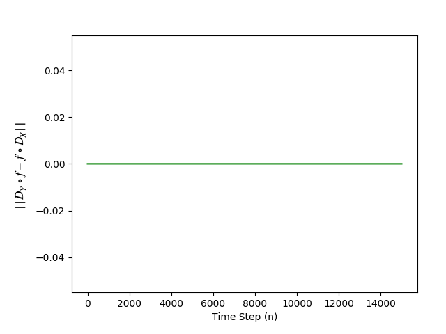
Figure 3. Relatedness for example 5.3

Example 5.4.

Recall that in the coupled cell network formalism of Golubitsky, Stewart and their collaborators all the invariant submanifolds are vector subspaces and their inclusions are, of course, linear. The formalism developed in [2, 3] is more general. There the maps between dynamical systems are projections followed by diagonal embeddings. In the case where the phase spaces are coordinate vector spaces all the maps are again linear. Consequently as we proved in Theorem 3.1 explicit RK methods work well for these types of networks.

The approach of [3] is generalized in [6] in several directions. In particular maps between dynamical systems constructed in [6] need not be linear. Consider the map

$$f:\mathbb{R}\to\mathbb{R}^{2},\qquad f(x)=(x^{2},x).$$

We claim that for any function $g:\mathbb{R}^{2}\to\mathbb{R}$ there are vector fields $X:\mathbb{R}\to\mathbb{R}$ and $Y:\mathbb{R}^{2}\to\mathbb{R}^{2}$ which are $f$-related. Indeed let

$$X(x)=xg(x^{2},x^{2})$$

and let

$$Y(y_{1},y_{2})=(2y_{1}g(y_{1},y_{2}^{2}),y_{2}g(y_{2}^{2},y_{1})).$$

Then

$$Y(f(x))=Y(x^{2},x)=(2x^{2}g(x^{2},x^{2}),xg(x^{2},x^{2})),$$

$$Tf_{x}=(2x,1)$$

and

$$Tf_{x}X(x)=(2x^{2}g(x^{2},x^{2}),xg(x^{2},x^{2}))=Y(f(x))$$

for all $x\in\mathbb{R}$. It follows that the parabola

$$P:=\{(x_{1},x_{2})\in\mathbb{R}^{2}\mid x_{2}^{2}=x_{1}\},$$

the image of $f$, is an invariant submanifold of the vector field $Y$. We present two simulations demonstrating that the parabola is not preserved under numerics, the first where $g(x,y)=0.999+\sin(x+y)+\frac{1}{x+y}$, and the second where $g(x,y)\equiv 1$:

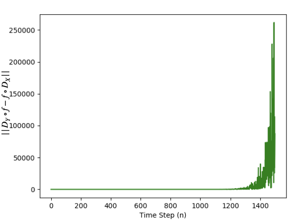
(a) $g(x,y)=0.999+\sin(x+y)+\frac{1}{x+y}$

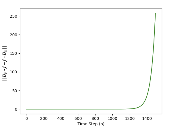
(b) $g(x,y)\equiv 1$

Figure 4. Non-invariance of parabola

Example 5.5.

Now we present an instance of theorem 3.1 with a nontrivial linear map $A:\mathbb{R}^{2}\rightarrow\mathbb{R}^{2}$, given by $A=\begin{pmatrix}1&-1\\ 1&1\end{pmatrix}$. Let $X=\begin{pmatrix}0&-1\\ 1&0\end{pmatrix}$ and $Y=\begin{pmatrix}1&0\\ 0&-1\end{pmatrix}$ be linear vector fields on $\mathbb{R}^{2}$. A quick calculation shows that $Y\circ A=A\circ X$, and hence that $(X,Y)$ are $A$-related. Theorem 3.1 tells us that numerics should agree, and they would with infinite precision numerics. However, while we see numerical agreement for many time steps, it appears that errors begin to arise after many more.

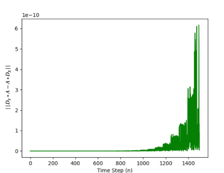
Figure 5. Relatedness for example 5.5

References

- [1] H.D. Brown, Near Algebras, PhD thesis, Ohio State Univ., 1966.
- [2] L. DeVille and E. Lerman, Modular dynamical systems on networks, J. Eur. Math. Soc. 17 (2015), no. 12, 2977–3013. arXiv:1303.3907 [math.DS]
- [3] L. DeVille and E. Lerman, Dynamics on networks of manifolds, SIGMA 11 (2015), Paper 022, 21 pp. arXiv:1208.1513 [math.DS]
- [4] M. Golubitsky, I. Stewart and A. Török, Patterns of synchrony in coupled cell networks with multiple arrows. SIAM J. Appl. Dyn. Syst., 4(1):78–100 (electronic), 2005.
- [5] A. Iserles, A first course in the numerical analysis of differential equations, Cambridge Texts in Applied Mathematics, Cambridge University Press, Cambridge, 1996. MR 1384977
- [6] E. Lerman, Networks of open systems, J. Geom. Phys. 130 (2018), 81–112; arXiv:1705.04814 [math.OC]
- [7] R.I. McLachlan, R.I. and G.R.W. Quispel, Geometric integrators for ODEs. Journal of Physics A: Mathematical and General ,39 (2006), p.5251-5285.
- [8] I. Stewart, M. Golubitsky and M. Pivato, Symmetry groupoids and patterns of synchrony in coupled cell networks, SIAM Journal on Applied Dynamical Systems 2 (2003), no. 4, 609–646.
- [9] Endre Süli and David F. Mayers, An introduction to numerical analysis, Cambridge University Press, Cambridge, 2003. MR 2006500
- [10] F.W. Warner, Foundations of differentiable manifolds and Lie groups, Springer-Verlag, New York Berlin Heidelberg Tokyo, 1983.