smooth	gradient dominated
distributed zero-order (nonconvex)	Alg. 1, this paper ($2$-point + DGD)	$\quad O\!\left(\!\sqrt{\dfrac{d}{m}}\log m\!\right)$	$O\!\left(\dfrac{d}{m}\right)$
	Alg. 2, this paper ($2d$-point + gradient tracking)	$O\!\left(\dfrac{d}{m}\right)$	$O\!\left(\!\left[1-c\big{(}1-\rho^{2}\big{)}^{2}\left(\dfrac{\mu}{L}\right)^{\frac{4}{3}}\right]^{m/d}\right)$
	ZONE [hajinezhad2019zone]	$O\left(\dfrac{\gamma(d)}{\sqrt{M}}\right)$	—
distributed first-order	DGD	$O\!\left(\dfrac{\log t}{\sqrt{t}}\right)$ [chen2012fast, zeng2018nonconvex] (convex)	$O\!\left(\dfrac{1}{t}\right)$ [olshevsky2019non] (strongly convex)
		$O\!\left(\!\dfrac{1}{\sqrt{T}}\!\right)$ [lian2017can] (nonconvex)
	2.3cmgradient
tracking	$O\!\left(\dfrac{1}{t}\right)$ [scutari2019distributed] (nonconvex)	$O\!\left(\!\left[1\!-\!c(1\!-\!\rho)^{2}\!\left(\dfrac{\mu}{L}\right)^{\!\frac{3}{2}}\right]^{\!t}\right)$ [nedic2017achieving] (strongly convex)
centralized zero-order	2.7cm[nesterov2017random]
($2$-point estimator)	$O\!\left(\dfrac{d}{m}\right)$ (nonconvex)	$O\!\left(\!\left[1\!-\!\dfrac{c}{d}\dfrac{\mu}{L}\right]^{m}\right)$ (strongly convex)
Note: The table summarizes best known convergence rates for deterministic nonconvex unconstrained optimization with 1) smooth,
Note: 2) gradient dominated objectives. The convex counterparts are listed if results for nonconvex cases have not been established.
Note: $m$ denotes the number of function value queries, $t$ denotes the number of iterations, $d$ denotes the dimension of the decision
Note: variable, $c$’s represent numerical constants that can be different for different algorithms.
Note: $M$ denotes the total number of function value queries and $T$ denotes the total number of iterations provided before the
Note: optimization procedure. The rates in [hajinezhad2019zone] and [lian2017can] assume constant step sizes chosen based on $M$ or $T$.
Note: The listed convergence rates are the ergodic rates of $\|\nabla f\|^{2}$ for the smooth case, and the objective error rates for the
Note: gradient dominated case, respectively.
Note: The rates provided in [hajinezhad2019zone] do not include explicit dependence on $d$; we use $\gamma(d)$ to denote this dependence.
Note: The cited results in this table may apply to more general settings (e.g., stochastic gradients [lian2017can, olshevsky2019non]).
Note: We do not include algorithms with Nesterov-type acceleration in this comparison.

Distributed multi-agent optimization lies at the core of a wide range of applications, and a large body of literature has been contributed to distributed multi-agent optimization algorithms. One line of research combines (sub)gradient-based methods with a consensus/averaging scheme, where each iteration of a local agent consists of one or multiple consensus steps and a local gradient evaluation step. It has been shown that, for convex functions, the convergence rates of distributed gradient-based algorithms can match or nearly match those of centralized gradient-based algorithms. Specifically, [nedic2009distributed, chen2012fast] proposed and analyzed consensus-based decentralized gradient descent (DGD) algorithms with $O(\log t/\sqrt{t})$ convergence for nonsmooth convex functions; [shi2015extra, nedic2017achieving, qu2018harnessing] employed the gradient tracking scheme and showed that the DGD with gradient tracking achieves $O(1/t)$ convergence for smooth convex functions and linear convergence for strongly convex functions; [qu2019accelerated] employed Nesterov’s gradient descent method and showed $O(1/t^{1.4-\epsilon})$ convergence for smooth convex functions and improved linear convergence for strongly convex functions where $\epsilon$ is an arbitrarily small positive number. Besides convergence rates, some works have additional focuses such as time-varying/directed graphs [nedic2014distributed], uncoordinated step sizes [xu2015augmented], stochastic (sub)gradient [ram2010distributed], etc.

While distributed convex optimization has broad applicability, nonconvex problems also appear in important applications such as distributed learning [omidshafiei2017deep], robotic networks [charrow2014cooperative], operation of wind farms [marden2013model], etc. Several works have considered nonconvex multi-agent optimization and developed various distributed gradient-based methods to converge to stationary points with convergence rate analysis, e.g., [di2016next, lian2017can, zeng2018nonconvex, scutari2019distributed]. We notice that for smooth functions, either convex or nonconvex, in general DGD with gradient-tracking converges faster than the method without gradient tracking, and its convergence rate has the same big-O dependence on the number of iterations as the centralized vanilla gradient descent method (See Table LABEL:tab:main_results).

Further, there has been increasing interest in zero-order optimization, where one does not have access to the gradient of the objective. Such situations can occur, for example, when only black-box procedures are available for computing the values of the functional characteristics of the problem, or when resource limitations restrict the use of fast or automatic differentiation techniques. Many existing works [kiefer1952stochastic, flaxman2005online, bach2016highly, nesterov2017random, duchi2015optimal] on zero-order optimization are based on constructing gradient estimators using finitely many function evaluations, e.g., gradient estimator based on Kiefer-Wolfowitz scheme[kiefer1952stochastic] by using $2d$-point function evaluations where $d$ is the dimension of the problem. However, this estimator does not scale up well with high-dimensional problems. [flaxman2005online] proposed and analyzed a single-point gradient estimator, and [bach2016highly] further studied the convergence rate for highly smooth objectives. [nesterov2017random] proposed two-point gradient estimators and showed that the convergence rates of the resulting algorithms are comparable to their first-order counterpart (See Table I). For instance, gradient descent with two-point gradient estimators converges with a rate of $O(d/m)$ where $m$ denotes the number of function value queries. [duchi2015optimal] and [shamir2017optimal] showed that two-point gradient estimators achieve the optimal rate $O(\sqrt{d/m})$ of stochastic zero-order convex optimization.

Some recent works have started to combine zero-order and distributed optimization methods [hajinezhad2019zone, sahu2018distributed, yu2019distributed]. For example, [hajinezhad2019zone] proposed the ZONE algorithm for stochastic nonconvex problems based on the method of multipliers. [sahu2018distributed] proposed a distributed zero-order algorithm over random networks and established its convergence for strongly convex objectives. [yu2019distributed] considered distributed zero-order methods for constrained convex optimization. However, there are still many questions remaining to be studied in distributed zero-order optimization. In particular, how do zero-order and distributed methods affect the performance of each other, and could their fundamental structural properties be kept when combining the two? For instance, it would be ideal if we could combine both $2$-point zero-order methods with DGD with gradient tracking and maintain the nice properties for both methods, leading to an “optimal” distributed zero-order algorithm if possible. This is unclear a prior, and indeed, as we shall show later, $2$-point gradient estimator and DGD with gradient tracking do not reconcile with each other well.

Contributions.

Motivated by the above observations, we propose two distributed zero-order algorithms: Algorithm 1 is based on the $2$-point estimator and DGD; Algorithm 2 is based on the $2d$-point gradient estimator and DGD with gradient tracking. We analyze the performance of the two algorithms for deterministic nonconvex optimization, and compare their convergence rates with their distributed first-order and centralized zero-order counterparts. The convergence rates of the two algorithms are summarized in Table LABEL:tab:main_results. Specifically, it can be seen that the rates of Algorithm 1 are comparable with the first-order decentralized gradient descent but are inferior to the centralized zero-order method; the rates of Algorithm 2 are comparable with the centralized zero-order method and the first-order DGD with gradient tracking. On the other hand, Algorithm 1 uses the $2$-point gradient estimator that requires only $2$ function value queries, while Algorithm 2 employs the $2d$-gradient estimator whose computation involves $2d$ function value queries, indicating that Algorithm 1 could be favored for high-dimensional problems even though its convergence is slower asymptotically, while Algorithm 2 could handle problems of relatively low dimensions better with faster convergence. These results shed light on how zero-order evaluations affect distributed optimization and how the presence of network structure affects zero-order algorithms. Different problems and different computation requirements would favor different integration of zero-order methods and distributed methods.

Compared to existing literature on distributed zero-order optimization, our Algorithm 1 is similar to the algorithms proposed in [sahu2018distributed, yu2019distributed], but our analysis assumes nonconvex objectives and also considers gradient dominated functions. While [hajinezhad2019zone] analyzed the performance of the ZONE algorithm for unconstrained nonconvex problems, we shall see that our Algorithm 1 achieves comparable convergence behavior with ZONE-M, and Algorithm 2 converges faster than ZONE-M in the deterministic setting due to the use of the gradient tracking technique. A more detailed comparison will be given in Section 3.4.

Notation.

We denote the $\ell_{2}$-norm of vectors and matrices by $\|\cdot\|$. The standard basis of $\mathbb{R}^{d}$ will be denoted by $\{e_{k}\}_{k=1}^{d}$. We let $\mathbf{1}_{n}\in\mathbb{R}^{n}$ denote the vector of all ones. We let $\mathbb{B}_{d}$ denote the closed unit ball in $\mathbb{R}^{d}$, and let $\mathbb{S}_{d-1}\coloneqq\{x\in\mathbb{R}^{d}:\|x\|=1\}$ denote the unit sphere. The uniform distributions over $\mathbb{B}_{d}$ and $\mathbb{S}_{d-1}$ will be denoted by $\mathcal{U}(\mathbb{B}_{d})$ and $\mathcal{U}(\mathbb{S}_{d-1})$. $I_{d}$ denotes the $d\times d$ identity matrix. For two matrices $A=[a_{ij}]\in\mathbb{R}^{p\times q}$ and $B=[b_{ij}]\in\mathbb{R}^{r\times s}$, their tensor product $A\otimes B$ is A⊗B = [a11B ⋯a1qB ⋮⋱⋮ap1B ⋯apqB ] ∈R^pr×qs.

2 Formulation and Algorithms

2.1 Problem Formulation

Let $\mathcal{N}=\{1,2,\ldots,n\}$ be the set of agents. Suppose the agents are connected by a communication network, whose topology is represented by an undirected, connected graph $\mathcal{G}=(\mathcal{N},\mathcal{E})$ where the edges in $\mathcal{E}$ represent communication links.

Each agent $i$ is associated with a local objective function $f_{i}:\mathbb{R}^{d}\rightarrow\mathbb{R}$. The goal of the agents is to collaboratively solve the optimization problem

$$\min_{x\in\mathbb{R}^{d}}\ \ f(x)\coloneqq\frac{1}{n}\sum_{i=1}^{n}f_{i}(x).$$ (1)

We assume that at each time step, agent $i$ can only query the function values of $f_{i}$ at finitely many points, and can only communicate with its neighbors. Similar to [nesterov2017random] and other works on zero-order optimization, we assume a deterministic setting where the queries of the function values are noise-free and error-free. The analysis of the deterministic setting will provide a baseline for extension to stochastic optimization which we leave as future work.

The following definitions will be useful later in the paper.

Definition 1.

1. A function $f:\mathbb{R}^{d}\rightarrow\mathbb{R}$ is said to be $L$-smooth if $f$ is continuously differentiable and satisfies ∥∇f(x)-∇f(y)∥≤L∥x-y∥,   ∀x,y∈R^d.

2. A function $f:\mathbb{R}^{d}\rightarrow\mathbb{R}$ is said to be $G$-Lipschitz if |f(x)-f(y)|≤G∥x-y∥   ∀x,y∈R^d.

3. A function $f:\mathbb{R}^{d}\rightarrow\mathbb{R}$ is said to be $\mu$-gradient dominated if $f$ is differentiable, has a global minimizer $x^{\ast}$, and 2μ(f(x)-f(x^∗)) ≤∥∇f(x)∥^2   ∀x∈R^d.

The notion of gradient domination is also known as Polyak-Łojasiewicz (PL) inequality, first introduced by [polyak1963gradient] and [lojasiewicz1963topological]. It can be viewed as a nonconvex analogy of strong convexity, as the centralized vanilla gradient descent achieves linear convergence for gradient dominated objective functions. The gradient domination condition has been frequently discussed in nonconvex optimization [polyak1963gradient, karimi2016linear]. Also, nonconvex but gradient dominated objective functions appear in many applications, e.g., linear quadratic control problems [fazel2018global] and deep linear neural networks [shamir2018exponential].

2.2 Preliminaries on Zero-Order and Distributed Optimization

We present some preliminaries to motivate our algorithm development.

Zero-order optimization based on gradient estimation. In zero-order optimization, one tries to minimize a function with the limitation that only function values at finitely many points may be obtained. One basic approach of designing zero-order optimization algorithms is to construct gradient estimators from zero-order information and substitute them for the true gradients. Here we introduce two types of zero-order gradient estimators for the noiseless setting:

1. The $2d$-point gradient estimator is given by

   $$\mathsf{G}^{(2d)}_{f}(x;u)=\sum_{k=1}^{d}\frac{f(x+ue_{k})-f(x-ue_{k})}{2u}e_{k},$$ (2)

   where $u$ is some given positive number. Basically, it approximates the gradient $\nabla f(x)$ by taking finite differences along $d$ orthogonal directions, and can be viewed as a noise-free version of the classical Kiefer-Wolfowitz type method [kiefer1952stochastic]. Given an $L$-smooth function $f:\mathbb{R}^{d}\rightarrow\mathbb{R}$, it can be shown that

   $$\|\mathsf{G}^{(2d)}_{f}(x;u)-\nabla f(x)\|\leq\mfrac{1}{2}uL\sqrt{d}$$

   for any $x\in\mathbb{R}^{d}$. The right-hand side decreases to zero as $u\rightarrow 0$. In other words, $\mathsf{G}^{(2d)}_{f}(x;u)$ can be arbitrarily close to $\nabla f(x)$ (as long as the finite differences can be evaluated accurately). One drawback of this estimator is that it requires $2d$ zero-order queries, which may not be computationally efficient for high-dimensional problems.

2. The $2$-point gradient estimator is given by

   $$\mathsf{G}^{(2)}_{f}(x;u,z)\coloneqq d\cdot\frac{f(x+uz)-f(x-uz)}{2u}z,$$ (3)

   where $z\in\mathbb{R}^{d}$ is a random vector that is sampled from the distribution $\mathcal{U}(\mathbb{S}_{d-1})$, and $u>0$ is a given positive number. The following proposition indicates that when $z$ is uniformly sampled from the sphere $\mathbb{S}_{d-1}$, the expectation of $\mathsf{G}^{(2)}_{f}(x;u,z)$ is the gradient of a “locally averaged” version of $f$.

   Proposition 1 ([flaxman2005online]).

   Suppose $f:\mathbb{R}^{d}\rightarrow\mathbb{R}$ is $L$-smooth. Then for any $u>0$ and $x\in\mathbb{R}^{d}$, E_z∼U(S_d-1) ​[G^(2)_f(x;u,z)] =∇f^u(x), where $f^{u}(x)\coloneqq\mathbb{E}_{y\sim\mathcal{U}(\mathbb{B}_{d})}\left[f(x+uy)\right]$.

   It has been shown in [nesterov2017random] that if we substitute $\mathsf{G}^{(2)}_{f}(x;u,z)$ for the gradient in the gradient descent algorithm, we have 1t∑_τ=0^t-1∥∇f(x_τ)∥^2 =O​(dm) for nonconvex smooth objectives, and f(x_τ)-f^∗= O​(​[1-c μ/Ld]^​m) for smooth and strongly convex objectives, where $x_{\tau}$ denotes the $\tau$’th iterate and $m$ denotes the number of zero-order queries in $t$ iterations (see Table LABEL:tab:main_results). These rates are comparable to the rates of the (centralized) vanilla gradient descent method, i.e., $O(1/t)$ for nonconvex smooth objectives and linear convergence for smooth and strongly convex objectives.

Distributed optimization. In this paper, we mainly focus on consensus-based algorithms for distributed optimization, where each agent maintains a local copy of the global variables, and weighs its neighbors’ information to updates its own local variable. Specifically, for a time-invariant and bidirectional communication network, we introduce a consensus matrix $W=[W_{ij}]\in\mathbb{R}^{n\times n}$ that satisfies the following assumption:

Assumption 1.

1. $W$ is a doubly stochastic matrix.

2. $W_{ii}>0$ for all $i\in\mathcal{N}$, and for two distinct agents $i$ and $j$, $W_{ij}>0$ if and only if $(i,j)\in\mathcal{E}$.

When Assumption 1 is satisfied, we have [qu2018harnessing]

$$\rho\coloneqq\left\|W-n^{-1}\mathbf{1}_{n}\mathbf{1}_{n}^{\top}\right\|<1.$$ (4)

We present two consensus-based algorithms that will serve as the basis for designing distributed zero-order algorithms.

1. The decentralized gradient descent (DGD) algorithm [nedic2009distributed, chen2012fast] is given by the following iterations:

   $$x^{i}(t)=\sum_{j=1}^{n}W_{ij}x^{j}(t-1)-\eta_{t}\nabla f_{i}(x^{i}(t-1)),$$ (5)

   where $x^{i}(t)\in\mathbb{R}^{d}$ denotes the local copy of the decision variable for the $i$’th agent, and $\eta_{t}$ is the step size. It has been shown that DGD in general converges more slowly than the centralized gradient descent algorithm [chen2012fast, qu2018harnessing] for smooth functions. This is because the local gradient $\nabla f_{i}$ does not vanish at the stationary point, and a diminishing step size $\eta_{t}$ is necessary, which slows down the convergence.

2. The DGD gradient tracking method incorporates additional local variables $s^{i}(t)$ to track the global gradient $\nabla f=\frac{1}{n}\sum_{i}\nabla f_{i}$: si(t)=∑j=1nWijsj(t​-​1) + ∇fi(xi(t​-​1))-∇fi(xi(t​-​2)), xi(t)=∑j=1nWijxj(t​-​1)-ηtsi(t), where we set $s^{i}(0)=\nabla f_{i}(x^{i}(0))$ for each $i$. Since gradient tracking has been proposed, it has attracted much attention and inspired many recent studies [xu2015augmented, di2016next, nedic2017achieving, qu2018harnessing, scutari2019distributed], as it can accelerate the convergence for smooth objectives compared to DGD. Here we provide a high level explanation of how gradient tracking works: For smooth functions, when $x^{i}(t)$ approaches consensus, $\nabla f_{i}(x^{i}(t))$ will not change much because of the smoothness, and therefore the local variables $s^{i}(t)$ will eventually reach a consensus; on the other hand, by induction it can be shown that 1n∑_i=1^n s^i(t) =1n∑_i=1^n ∇f_i(x^i(t)). Therefore, the sequence $(s^{i}(t))_{t\in\mathbb{N}}$ will eventually converge to the global gradient, and a constant stepsize $\eta_{t}=\eta$ is allowed, leading to comparable convergence rates as the centralized gradient methods. See [qu2018harnessing, Section III and Section IV.B] for more discussion.

2.3 Our Algorithms

Following the previous discussions, it would be ideal if we can combine the $2$-point gradient estimator and the DGD with gradient tracking and maintain a convergence rate comparable to the centralized vanilla gradient descent method. However, it turns out that such combination does not lead to the desired convergence rate. This is mainly because gradient tracking requires increasingly accurate local gradient information as one approaches the stationary point to achieve faster convergence compared to DGD, whereas the $2$-point gradient estimator can produce a variance that does not decrease to zero even if the radius $u$ decreases to zero; a more detailed explanation will be provided in Section 3.3.

We propose the following two distributed zero-order algorithms for the problem (1):

for $t=1,2,3,\ldots$ do

       foreach $i\in\mathcal{N}$ do

1. Generate $z^{i}(t)\sim\mathcal{U}(\mathbb{S}_{d-1})$ independently from $(z^{i}(\tau))_{\tau=1}^{t-1}$ and $(z^{j}(\tau))_{\tau=1}^{t}$ for $j\neq i$.

Update $x^{i}(t)$ by

$$g^{i}(t) =\mathsf{G}_{f_{i}}^{(2)}(x^{i}(t-1);u_{t},z^{i}(t)),$$ (6)

$$x^{i}(t) =\sum_{j=1}^{n}W_{ij}(x^{j}(t-1)-\eta_{t}g^{j}(t)).$$ (7)

             end foreach

            

             end for

Algorithm 1 2-point gradient estimator without global gradient tracking

Set $s^{i}(0)=g^{i}(0)=0$ for each $i\in\mathcal{N}$.

for $t=1,2,3,\ldots$ do

       foreach $i\in\mathcal{N}$ do

            

1. Update $s^{i}(t)$ by

   $$g^{i}(t) =\mathsf{G}^{(2d)}_{f_{i}}(x^{i}(t-1);u_{t}),$$ (8)

   $$s^{i}(t) =\!\sum_{j=1}^{n}W_{ij}\!\left(s^{j}(t\!-\!1)\!+\!g^{j}(t)\!-\!g^{j}(t\!-\!1)\right)\!.$$ (9)

2. Update $x^{i}(t)$ by

   $$x^{i}(t)=\sum_{j=1}^{n}W_{ij}(x^{j}(t-1)-\eta s^{j}(t)).\phantom{XXX}$$ (10)

             end foreach

            

             end for

Algorithm 2 $2d$-point gradient estimator with global gradient tracking

1. Algorithm 1 employs the $2$-point gradient estimator (3), and adopts the consensus procedure of the DGD algorithm that only involves averaging over the local decision variables.

2. Algorithm 2 employs the $2d$-point gradient estimator (2), and adopts the consensus procedure of the gradient tracking method where the auxiliary variable $s^{i}(t)$ is introduced to track the global gradient $\nabla f=\frac{1}{n}\sum_{i}\nabla f_{i}$. We shall see in Theorems 3 and 4 that $s^{i}(t)$ converges to the gradient of the global objective function as $t\rightarrow\infty$ under mild conditions.

3 Main Results

In this section we present the convergence results of our algorithms. The proofs are postponed to the Appendix.

3.1 Convergence of Algorithm 1

Let $x^{i}(t)$ denote the sequence generated by Algorithm 1 with a positive, non-increasing sequence of step sizes $\eta_{t}$. Denote ¯x(t)≔1n∑_i=1^n x^i(t),   R_0≔1n∑_i=1^n∥x^i(0)-¯x(0)∥^2.

We first analyze the case with general nonconvex smooth objective functions.

Theorem 1.

Assume that each local objective function $f_{i}$ is uniformly $G$-Lipschitz and $L$-smooth for some positive constants $G$ and $L$, and that $f^{\ast}\coloneqq\inf_{x\in\mathbb{R}^{d}}f(x)>-\infty$.

1. Suppose $\eta_{1}L\leq 1/4$, $\sum_{t=1}^{\infty}\eta_{t}=+\infty$, $\sum_{t=1}^{\infty}\eta_{t}^{2}<+\infty$, and $\sum_{t=1}^{\infty}\eta_{t}u_{t}^{2}<+\infty$. Then almost surely, $\|x^{i}(t)-\bar{x}(t)\|$ converges to zero for all $i\in\mathcal{N}$, $\nabla f(\bar{x}(t))$ converges to zero, and $\lim_{t\rightarrow\infty}f(\bar{x}(t))$ exists.

2. Suppose that

   $$\eta_{t}=\frac{\alpha_{\eta}}{4L\sqrt{d}}\cdot\frac{1}{\sqrt{t}},\qquad u_{t}\leq\frac{\alpha_{u}G}{L\sqrt{d}}\cdot\frac{1}{t^{\gamma/2-1/4}}$$

   with $\alpha_{\eta}\in(0,1]$, $\alpha_{u}\geq 0$ and $\gamma>1$. Then almost surely, $\|x^{i}(t)-\bar{x}(t)\|$ converges to zero for all $i$, and $\liminf_{t\rightarrow\infty}\|\nabla f(\bar{x}(t))\|=0$. Furthermore, we have

   $$\frac{\sum_{\tau=0}^{t-1}\!\eta_{\tau+1}\mathbb{E}\!\left[\|\nabla f(\bar{x}(\tau))\|^{2}\right]}{\sum_{\tau=0}^{t-1}\eta_{\tau+1}}\leq \sqrt{\frac{d}{t}}\Bigg{[}\frac{\alpha_{\eta}G^{2}}{3n^{2}}\ln(2t\!+\!1)\!+\!\frac{8L(f(\bar{x}(0))\!\!-\!\!f^{\ast})}{\alpha_{\eta}}\!+\!\frac{6R_{0}L^{2}}{(1\!-\!\rho^{2})\sqrt{d}}$$ (11)

   $$\qquad\qquad+\frac{9\alpha_{\eta}^{2}\kappa^{2}\rho^{2}G^{2}}{4(1\!-\!\rho^{2})^{2}\sqrt{d}}+\frac{9\alpha_{u}^{2}\gamma G^{2}}{4(\gamma\!-\!1)}\Bigg{]}+o\!\left(\!\frac{1}{\sqrt{t}}\!\right),$$

   where $\kappa$ is some positive numerical constant, and

   $$\frac{1}{n}\sum_{i=1}^{n}\mathbb{E}\!\left[\|x^{i}(t)-\bar{x}(t)\|^{2}\right]\leq\frac{\alpha_{\eta}^{2}\kappa^{2}\rho^{2}}{4(1-\rho^{2})^{2}}\frac{G^{2}/L^{2}}{t}+o(t^{-1}).$$ (12)

Remark 1.

Note that in (11), we use the squared norm of the gradient to assess the sub-optimality of the iterates, and characterize the convergence by ergodic rates. This type of convergence rate bound is common for local methods of unconstrained nonconvex problems where we do not aim for global optimal solutions [ghadimi2013stochastic, nesterov2017random].

Remark 2.

Each iteration of Algorithm 1 requires $2$ queries of function values. Thus the convergence rate (11) can also be interpreted as $O(\sqrt{d/m}\log m)$ where $m$ denotes the number of function value queries. Characterizing convergence rate in terms of the number of function value queries $m$ and the dimension $d$ is conventional for zero-order optimization. In scenarios where zero-order methods are applied, the computation of the function values is usually one of the most time-consuming procedures. In addition, it is also of interest to characterize how the convergence scales with the dimension $d$.

The next theorem shows that for a gradient dominated global objective, a better convergence rate can be achieved.

Theorem 2.

Assume that each local objective function $f_{i}$ is uniformly $L$-smooth for some $L>0$. Furthermore, assume that $\inf_{x\in\mathbb{R}^{d}}f_{i}(x)=f_{i}^{\ast}>-\infty$ for each $i$, and that the global objective function $f$ is $\mu$-gradient dominated and has a minimum value denoted by $f^{\ast}$. Suppose

$$\eta_{t}=\frac{2\alpha_{\eta}}{\mu(t+t_{0})},\quad u_{t}\leq\frac{\alpha_{u}}{\sqrt{t+t_{0}}}$$

for some $\alpha_{\eta}>1$ and $\alpha_{u}>0$, where t_0≥2αηLμ(1​-​ρ2) ​( 32Ld3μ+ 9ρ) -1. Then, using Algorithm 1, we have

$$\mathbb{E}\!\left[f(\bar{x}(t))\!-\!f^{\ast}\right]\leq\ \!\left(\!\frac{32\alpha_{\eta}^{2}L^{2}\Delta}{\mu^{2}}+\frac{6\alpha_{\eta}\alpha_{u}^{2}L^{2}}{\mu}\!\right)\!\frac{d}{t}+o(t^{-1}),$$ (13)

$$\frac{1}{n}\!\sum_{i=1}^{n}\!\mathbb{E}\!\left[\|x^{i}(t)\!-\!\bar{x}(t)\|^{2}\right]\leq\ \frac{32\alpha_{\eta}^{2}\rho^{2}L\Delta}{\mu^{2}(1-\rho^{2})}\!\left(\frac{4d}{3}+\frac{6\rho^{2}}{1\!-\!\rho^{2}}\right)\!\frac{1}{t^{2}}+o(t^{-2}),$$ (14)

where $\Delta\coloneqq f^{\ast}-\frac{1}{n}\sum_{i=1}^{n}f^{\ast}_{i}$.

Remark 3.

The convergence rate (13) can also be described as $\mathbb{E}[f(\bar{x}(t))-f^{\ast}]=O(d/m)$, where $m$ is the number of function value queries.

Table LABEL:tab:main_results shows that, while Algorithm 1 employs a randomized 2-point zero-order estimator of $\nabla f_{i}$, its convergence rates are comparable with the decentralized gradient descent (DGD) algorithm [lian2017can, nedic2016stochastic]. However, its convergence rates are inferior to its centralized zero-order counterpart in [nesterov2017random].

3.2 Convergence of Algorithm 2

Let $(x^{i}(t),s^{i}(t))$ denote the sequence generated by Algorithm 2 with a constant step size $\eta$. Denote ¯x(t) ≔1n∑_i=1^n x^i(t),     R_0 ≔1n∑_i=1^n​ (​ ηρ22L∥∇f_i(x^i(0))∥^2 ​+​∥x^i(0)-¯x(0)∥^2 ​) +ηρ2u12Ld4. We first analyze the case where the local objectives are nonconvex and smooth.

Theorem 3.

Assume that each local objective function $f_{i}$ is uniformly $L$-smooth for some positive constant $L$, and that $f^{\ast}\coloneqq\inf_{x\in\mathbb{R}^{d}}f(x)>-\infty$. Suppose ηL≤min{ 16, (1-ρ2)24ρ2(3+4ρ2)},  R_u≔d∑_t=1^∞u_t^2 <+∞, and that $u_{t}$ is non-increasing. Then $\lim_{t\rightarrow\infty}f(\bar{x}(t))$ exists,

$$\frac{1}{t}\sum_{\tau=0}^{t-1}\|\nabla f(\bar{x}(\tau))\|^{2}\leq \frac{1}{t}\left[\frac{3.2(f(\bar{x}(0))-f^{\ast})}{\eta}+\frac{12.8L^{2}R_{0}}{1-\rho^{2}}+2.4R_{u}L^{2}\right],$$ (15)

and

$$\frac{1}{t}\sum_{\tau=0}^{t-1}\frac{1}{n}\sum_{i=1}^{n}\|x^{i}(\tau)-\bar{x}(\tau)\|^{2}\leq\ \frac{1}{t}\!\left[1.6\eta(f(\bar{x}(0))-f^{\ast})+\frac{3.2R_{0}}{1-\rho^{2}}+0.35R_{u}\right],$$ (16)

$$\frac{1}{t}\!\sum_{\tau=1}^{t}\!\frac{1}{n}\!\sum_{i=1}^{n}\!\|s^{i}(\tau)\!-\!\nabla f(\bar{x}(\tau\!\!-\!\!1))\|^{2}\leq\ \frac{1}{t}\!\left[9.6L(f(\bar{x}(0))-f^{\ast})+\frac{19.2LR_{0}}{\eta(1-\rho^{2})}+\frac{2.35}{\eta}LR_{u}\right].$$ (17)

Remark 4.

Theorem 3 shows that Algorithm 2 achieves a convergence rate of $O(1/t)$ in terms of the averaged squared norm of $\nabla f(\bar{x}(t))$, and has a consensus rate of $O(1/t)$ for the averages of the squared consensus error $\|x^{i}(t)\!-\!\bar{x}(t)\|^{2}$ and the squared gradient tracking error $\|s^{i}(t)\!-\!\nabla f(\bar{x}(t\!-\!1))\|^{2}$. They match the rates for distributed nonconvex optimization with gradient tracking [scutari2019distributed]. On the other hand, since each iteration requires $2d$ queries of function values, we get a $O(d/m)$ rate in terms of the number of function value queries $m$. This matches the convergence rate of centralized zero-order algorithms without Nesterov-type acceleration [nesterov2017random].

Now we proceed to the situation with a gradient dominated global objective.

Theorem 4.

Assume that each local objective function $f_{i}$ is uniformly $L$-smooth for some positive constant $L$, and that the global objective function $f$ is $\mu$-gradient dominated and achieves it global minimum at $x^{\ast}$. Suppose the step size $\eta$ satisfies

$$\eta L=\alpha\cdot\left(\frac{\mu}{L}\right)^{\frac{1}{3}}\frac{(1-\rho^{2})^{2}}{14}$$ (18)

for some $\alpha\in(0,1]$, and $(u_{t})_{t\geq 1}$ is non-increasing. Let λ≔1-α(1-ρ25)^2 (μL)^43. Then

$$f(\bar{x}(t))-f(x^{\ast})\leq O(\lambda^{t})+5(1-\rho^{2})Ld\sum_{\tau=0}^{t-1}\lambda^{\tau}u^{2}_{t-\tau},$$ (19)

$$\frac{1}{n}\sum_{i=1}^{n}\|x^{i}(t)\!-\!\bar{x}(t)\|^{2}\leq O(\lambda^{t})+\frac{3\eta Ld}{1\!-\!\rho^{2}}\sum_{\tau=0}^{t-1}\lambda^{\tau}u^{2}_{t-\tau},$$ (20)

$$\frac{1}{n}\sum_{i=1}^{n}\|s^{i}(t)\!-\!\nabla f(\bar{x}(t\!-\!1))\|^{2}\leq O(\lambda^{t})+\frac{18L^{2}d}{1\!-\!\rho^{2}}\sum_{\tau=0}^{t-1}\lambda^{\tau}u_{t\!-\!\tau}^{2}.$$ (21)

Remark 5.

If we use an exponentially decreasing sequence $u_{t}\propto\tilde{\lambda}^{t/2}$ with $\tilde{\lambda}<\lambda$, then both the objective error $f(\bar{x}(t))-f(x^{\ast})$ and the consensus errors $\|x^{i}(t)-\bar{x}(t)\|^{2}$ and $\|s^{i}(t)-\nabla f(\bar{x}(t-1))\|^{2}$ achieve linear convergence rate $O(\lambda^{t})$, or $O(\lambda^{m/d})$ in terms of the number of function value queries. In addition, we notice that the decaying factor $\lambda$ given by Theorem 4 has a better dependence on $\mu/L$ than in [nedic2017achieving] for convex problems. We point out that this is not a result of using zero-order techniques, but rather a more refined analysis of the gradient tracking procedure.

Remark 6.

Note that the conditions on the step sizes in Theorems 2, 3 and 4 depend on $\rho$, a measure of the connectivity of the network. In order to choose step sizes to satisfy theses conditions in the distributed setting, one possible approach is as follows: Assuming that each agent knows an upper bound $\overline{n}$ on the total number of agents, by [olshevsky2017linear, Lemma 2], if one chooses $W$ to be the lazy Metropolis matrix, then $\rho\leq 1-1/(71\overline{n}^{2})$, based on which the agents can then derive their step sizes according to the conditions in the theorems. We also note that some existing works (e.g., [li2019decentralized]) attempt to get rid of the dependence of step sizes on the graph topology, and whether those techniques can be applied in our work is beyond the scope of this paper but is an interesting future direction.

3.3 Comparison of the Two Algorithms

We see from the above results that Algorithm 2 converges faster than Algorithm 1 asymptotically as $m\rightarrow\infty$ in theory. However, each iteration of Algorithm 2 makes progress only after $2d$ queries of function values, which could be an issue if $d$ is very large. On the contrary, each iteration of Algorithm 1 only requires $2$ function value queries, meaning that progress can be made relatively immediately without exploring all the $d$ dimensions. This observation suggests that, when neglecting communication delays, Algorithm 1 is more favorable for high-dimensional problems, whereas Algorithm 2 could handle problems of relatively low dimensions better with faster convergence.

We emphasize that there still exists a trade-off between the convergence rate and the ability to handle high-dimensional problems even if one combines the $2$-point gradient estimator (2) with the gradient tracking method as

$$g^{i}(t) =\mathsf{G}^{(2)}_{f_{i}}(x^{i}(t-1);u_{t},z^{i}(t)),\ \ z^{i}(t)\sim\mathcal{U}(\mathbb{S}_{d-1}),$$ (22)

$$s^{i}(t) =\sum_{j=1}^{n}W_{ij}\!\left(s^{j}(t\!-\!1)+g^{j}(t)-g^{j}(t\!-\!1)\right).$$

$$x^{i}(t) =\sum_{j=1}^{n}W_{ij}(x^{j}(t-1)-\eta s^{j}(t)).$$

Theoretical analysis suggests that, in order for $s^{i}(t)$ to reach a consensus in the sense that $\mathbb{E}\!\left[\|s^{i}(t)\!-\!s^{j}(t)\|^{2}\right]\!$ converges to $0$, we need lim_t→∞E ​[ ∥g^i(t)-g^i(t-1)∥^2]→0. On the other hand, we have the following lemma regarding the variance of the $2$-point gradient estimator $\mathsf{G}^{(2)}_{f}(x;u,z)$.

Lemma 1.

Let $f:\mathbb{R}^{d}\rightarrow\mathbb{R}$ be an arbitrary $L$-smooth function. Then lim_u→0^+E_z ​[ ∥G^(2)_f(x;u,z)∥^2 ] =(d-1)∥∇f(x)∥^2, where $z\sim\mathcal{U}(\mathbb{S}_{d-1})$.

Proof.

Notice that for any $z\in\mathbb{S}_{d-1}$ and $u\in(0,1]$, we have |f(x​+​uz)-f(x​-​uz)2u| ≤sup_y∈B_d ∥∇f(x+y)∥. Therefore limu→0Ez​[∥G(2)f(x;u,z)∥2]=d2Ez​ [|limu→0f(x​+​uz) ​-​ f(x​-​uz)2u|2]​​= d2Ez​ [|∇f(x)⊤z |2]=d2∇f(x)⊤Ez​ [zz⊤]∇f(x) = d∥∇f(x)∥2, where in the second step we exchanged the order of limit and expectation by the bounded convergence theorem, and in the last step we used $d\,\mathbb{E}_{z}\!\left[zz^{\top}\right]=I_{d}$ for $z\sim\mathcal{U}(\mathbb{S}_{d-1})$. Then, noticing that $\nabla f^{u}(x)\rightarrow\nabla f(x)$ as $u\rightarrow 0$, we get limu→0Ez​[∥G(2)f(x;u,z) -∇fu(x)∥2]=limu→0(Ez​[∥G(2)f(x;u,z)∥2]-∥∇fu(x)∥2)=(d-1)∥∇f(x)∥2, which completes the proof. ∎

Lemma 1 suggests that, each gradient estimator $\mathsf{G}^{(2)}_{f_{i}}(x^{i}(t-1);u_{t},z^{i}(t))$ in (22) will produce a non-vanishing variance approximately equal to $(d-1)\,\mathbb{E}\!\left[\|\nabla f_{i}(x^{i}(t-1))\|^{2}\right]$ even if we let $u\rightarrow 0$ as $x^{i}(t)$ approaches a stationary point. Consequently, $\mathbb{E}\!\left[\|g^{i}(t)-g^{i}(t-1)\|^{2}\right]$ is not guaranteed to converge to zero as $t\rightarrow\infty$. The non-vanishing variance will then be reflected in $s^{i}(t)$ that tracks the global gradient, and consequently the overall convergence will be slowed down. We refer to [nedic2017achieving, qu2018harnessing, pu2018distributed] for related analysis, and to Section 4 for a numerical example.

3.4 Comparison with Existing Algorithms

In this subsection, we provide a detailed comparison with existing literature on distributed zero-order optimization, specifically [hajinezhad2019zone, sahu2018distributed, yu2019distributed].

1. References [sahu2018distributed, yu2019distributed] discuss convex problems, while [hajinezhad2019zone] and our work focus on nonconvex problems.

2. In terms of the assumptions on the noisy function queries, [yu2019distributed] and our work consider a noise-free case. [hajinezhad2019zone] considers stochastic queries but assumes two function values can be obtained for a single random sample. [sahu2018distributed] assumes independent additive noise on each function value query. We expect that our Algorithm 1 can be generalized to the setting adopted in [hajinezhad2019zone] with heavier mathematics. Extensions to general stochastic cases remain our ongoing work.

3. In terms of the approach to reach consensus among agents, our algorithms are similar to [sahu2018distributed, yu2019distributed], where some weighted average of the neighbors’ local variables is utilized, while [hajinezhad2019zone] uses the method of multipliers to design their algorithms. We also mention that, our Algorithm 2 employs the gradient tracking technique, which, to our best knowledge, has not been discussed in existing literature on distributed zero-order optimization yet.

4. Regarding the convergence rates for nonconvex optimization, [hajinezhad2019zone] proved that its proposed ZONE algorithm achieves $O(1/{T})$ rate if each iteration also employs $O(T)$ function value queries, where $T$ is the number of iterations planned in advance. Therefore in terms of the number of function value queries $M$, its convergence rate is in fact $O(1/{\sqrt{M}})$, which is roughly comparable with Algorithm 1 and slower than Algorithm 2 in our paper. Also, [hajinezhad2019zone] did not discuss the dependence on the problem dimension $d$. Moreover, our algorithms only require constant numbers ($2$ or $2d$) of function value queries which is more appealing for practical implementation when $T$ is set to be very large for achieving sufficiently accurate solutions.

4 Numerical Examples

We consider a multi-agent nonconvex optimization problem formulated as

$$\min_{x\in\mathbb{R}^{d}} \frac{1}{n}\sum_{i=1}^{n}f_{i}(x),$$ (23)

$$f_{i}(x)= \frac{a_{i}}{1+\exp(-\xi_{i}^{\top}x\!-\!\nu_{i})}+b_{i}\ln(1+\|x\|^{2}),$$

where $a_{i},b_{i},\nu_{i}\in\mathbb{R}$ and $\xi_{i}\in\mathbb{R}^{d}$ for each $i=1,\ldots,N$.

For the numerical example, we set the dimension to be $d=64$ and the number of agents to be $n=50$. The parameters $a_{i}$, $\nu_{i}$ and each entry of $\xi_{i}$ are randomly generated from the standard Gaussian distribution, and $(b_{1},\ldots,b_{n})$ is generated from the distribution $\mathcal{N}\big{(}\mathbf{1}_{n},I_{n}-\frac{1}{n}\mathbf{1}_{n}\mathbf{1}_{n}^{\top}\big{)}$ so that $\frac{1}{n}\sum_{i}b_{i}=1$. The graph $\mathcal{G}=(\mathcal{N},\mathcal{E})$ is generated by uniformly randomly sampling $n$ points on $\mathbb{S}_{2}$, and then connecting pairs of points with spherical distances less than $\pi/4$. The Metropolis-Hastings weights [xiao2005scheme] are employed for constructing $W$.

We compare the following algorithms on the problem (23):

1. Algorithm 1 with $\eta_{t}=0.02/\sqrt{t}$ and $u_{t}=4/\sqrt{t}$;

2. Algorithm 2 with $\eta=0.02$ and $u_{t}=4/t^{3/4}$;

3. ZONE-M [hajinezhad2019zone], where we test two setups $J=1$, $\rho_{t}=4\sqrt{t}$, $u_{t}=4/\sqrt{t}$ and $J=100$, $\rho_{t}=0.4\sqrt{t}$, $u_{t}=4/\sqrt{t}$;

4. $2$-point gradient estimator combined with gradient tracking [see (22)] with $\eta=2\times 10^{-4}$ and $u_{t}=4/t^{3/4}$.

All algorithms start from the same initial points, which are randomly generated from the distribution $\mathcal{N}(0,\frac{25}{d}I_{d})$ for each agent.

4.1 Comparison of Algorithm 1 and Algorithm 2

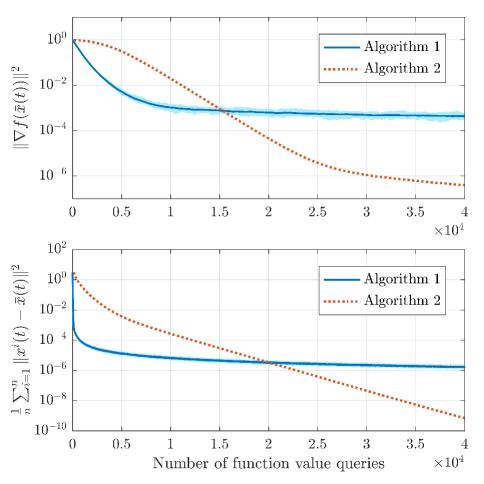
Figure 1: Convergence of Algorithm 1 and Algorithm 2. For Algorithm 1, the light blue shaded areas represent the results for $50$ random instances, and the dark blue curves represent their average.

Figure 1 shows the convergence behavior of Algorithm 1 and Algorithm 2, where the top figure illustrates the squared norm of the gradient at $\bar{x}(t)$, and the bottom figure illustrates the consensus error $\frac{1}{n}\sum_{i=1}^{n}\|x^{i}(t)-\bar{x}(t)\|^{2}$. The horizontal axis has been normalized as the number of function value queries $m$. We can see that Algorithm 1 converges faster during the initial stage, but then slows down and converges at a relatively stable sublinear rate. The convergence of Algorithm 2 is relatively slow initially, but then becomes faster as $m\gtrsim 0.5\times 10^{4}$, and when $m\gtrsim 2\times 10^{4}$, Algorithm 2 achieves smaller squared gradient norm and consensus error compared to Algorithm 1; the convergence slows down as $m$ exceeds $2.5\times 10^{4}$ but is still faster than Algorithm 1. Further investigation of the simulation results suggests that the speed-up of Algorithm 2 within $0.5\times 10^{4}\lesssim m\lesssim 2.5\times 10^{4}$ is due to $\bar{x}(t)$ becoming sufficiently close to a local optimal, around which the objective function is locally strongly convex; the slow-down after $m$ exceeds $2.5\times 10^{4}$ is caused by the zero-order gradient estimation error that becomes dominant, and can be postponed or avoided if we let $u_{t}$ decrease more aggressively.

From these results, it can be seen that, if the total number of function value queries is limited by, say $m\lesssim 1.5\times 10^{4}$, then Algorithm 1 might be favorable compared to Algorithm 2 despite slower asymptotic convergence rate, while if more function value queries are allowed, then Algorithm 2 could be favored. We observe that this is related with the discussion in Section 3.3.

4.2 Comparison with Other Algorithms

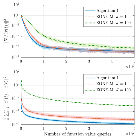
Figure 2: Convergence of Algorithm 1 and ZONE-M with $J=1$ and $J=100$. For each algorithm, the light shaded areas represent the results for $50$ random instances, and the dark curves represent their average.

Figure 2 compares the convergence of Algorithm 1 and the two setups of ZONE-M, including the curves for the squared norm of the gradient $\|\nabla f(\bar{x}(t))\|^{2}$ and the consensus error $\frac{1}{n}\sum_{i=1}^{n}\|x^{i}(t)-\bar{x}(t)\|^{2}$. The horizontal axis has been normalized as the number of function value queries $m$. It can be seen that Algorithm 1 and ZONE-M with $\rho_{t}\propto\sqrt{t},J=1$ have similar convergence behavior. For ZONE-M with $\rho_{t}\propto\sqrt{t}$ and $J=100$, while the convergence of $\|\nabla f(\bar{x}(t))\|^{2}$ is comparable with Algorithm 1 and ZONE-M with $J=1$, the consensus error decreases much slower, as ZONE-M with $J=100$ conducts much fewer consensus averaging steps per function value query compared to Algorithm 1 and ZONE-M with $J=1$.

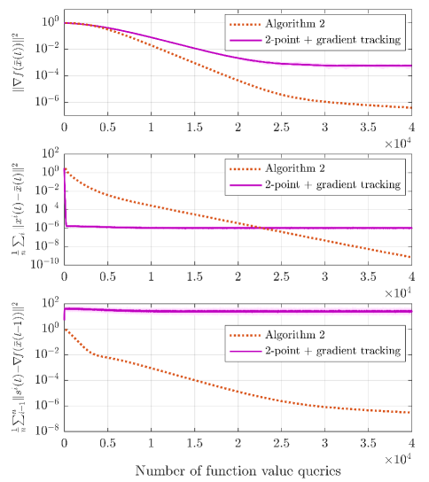
Figure 3: Convergence of Algorithm 2 and $2$-point estimator combined with gradient tracking. For $2$-point estimator combined with gradient tracking, the light pink shaded areas represent the results for $50$ random instances, and the dark purple curves represent their average.

Figure 3 compares the convergence of Algorithm 2 and the $2$-point estimator combined with gradient tracking (22), including the curves for the squared norm of the gradient $\|\nabla f(\bar{x}(t))\|^{2}$, the consensus error $\frac{1}{n}\sum_{i=1}^{n}\|x^{i}(t)-\bar{x}(t)\|^{2}$ and also the gradient tracking error $\frac{1}{n}\sum_{i=1}^{n}\|s^{i}(t)-\nabla f(\bar{x}(t\!-\!1))\|^{2}$. It’s straightforward to see that Algorithm 2 has better asymptotic convergence behavior than the $2$-point estimator combined with gradient tracking. Moreover, for the $2$-point estimator combined with gradient tracking, the gradient tracking error does not converge to zero but remains at a constant level, indicating that the gradient tracking technique is ineffective in this case. These observations are in accordance with our theoretical discussion in Section 3.3.

5 Conclusion

We proposed two distribtued zero-order algorithms for nonconvex multi-agent optimization, established theoretical results on their convergence rates, and showed that they achieve comparable performance with their distributed gradient-based or centralized zero-order counterparts. We also provided a brief discussion on how the dimension of the problem will affect their performance in practice. There are many lines of future work, such as 1) introducing noise or errors when evaluating $f_{i}(x)$, 2) investigating how to escape from saddle-point for distributed zero-order methods, 3) extension to nonsmooth problems, 4) investigating whether the step sizes can be independent of the network topology, 5) studying time-varying graphs, and 6) investigating the fundamental gap between centralized methods and distributed methods, especially for high-dimensional problems.

Appendix A Auxiliary Results for Convergence Analysis

Recall that $W\in\mathbb{R}^{n\times n}$ is a consensus matrix that satisfies Assumption 1 in the main text, and ρ:= ∥W-n^-11_n1_n^⊤∥<1. The following lemma is a standard result in consensus optimization.

Lemma 2.

For any $x^{1},\ldots,x^{n}\in\mathbb{R}^{d}$, we have ∥(W⊗I_d)(x-1_n⊗¯x)∥ ≤ρ∥x-1_n⊗¯x∥, where we denote x=[x1⋮xn],   ¯x=1n∑_i=1^n x^i.

The following lemma provides a useful property of smooth functions.

Lemma 3.

Suppose $f:\mathbb{R}^{p}\rightarrow\mathbb{R}$ is $L$-smooth and $\inf_{x\in\mathbb{R}^{p}}f(x)=f^{\ast}>-\infty$. Then ∥∇f(x)∥^2≤2L(f(x)-f^∗).

Proof.

The $L$-smoothness of $f$ implies f^∗≤f(x-L^-1∇f(x)) ≤f(x)-12L∥∇f(x)∥^2. ∎

For a $\mu$-gradient dominated and $L$-smooth function, we can see from Lemma 3 that $\mu\leq L$.

The following lemma will be used to establish convergence of the proposed algorithms.

Lemma 4 ([robbins1971convergence]).

Let $(\Omega,\mathcal{F},\mathbb{P})$ be a probability space and $(\mathcal{F}_{t})_{t\in\mathbb{N}}$ be a filtration. Let $U(t),\xi(t)$ and $\zeta(t)$ be nonnegative $\mathcal{F}_{t}$-measurable random variables for $t\in\mathbb{N}$ such that E​[U(t+1)|F_t] ≤U(t)+ξ(t)-ζ(t),  ∀t=0,1,2,… Then almost surely on the event $\{\sum_{t=0}^{\infty}\xi(t)<+\infty\}$, $U(t)$ converges to a random variable and $\sum_{t=0}^{\infty}\zeta(t)<+\infty$.

As a special case, let $U_{t}$, $\xi_{t}$ and $\zeta_{t}$ be (deterministic) nonnegative sequences for $t\in\mathbb{N}$ such that U_t+1 ≤U_t+ξ_t-ζ_t, with $\sum_{t=0}^{\infty}\xi_{t}<+\infty$. Then $U_{t}$ converges and $\sum_{t=0}^{\infty}\zeta_{t}<+\infty$.

We will extensively use the following properties of the distribution $\mathcal{U}(\mathbb{S}_{d-1})$:

$$\mathbb{E}_{z\sim\mathcal{U}(\mathbb{S}_{d-1})}\!\left[d\cdot\langle g,z\rangle z\right]=g,\qquad\mathbb{E}_{z\sim\mathcal{U}(\mathbb{S}_{d-1})}\!\left[d\cdot\langle g,z\rangle^{2}\right]=\|g\|^{2}$$ (24)

for any (deterministic) $g\in\mathbb{R}^{d}$.

The following results discuss the bias and the second moment of the $2$-point gradient estimator.

Lemma 5.

1. Let $u>0$ be arbitrary, and suppose $f:\mathbb{R}^{d}\rightarrow\mathbb{R}$ is differentiable. Then

   $$\mathbb{E}_{z\sim\mathcal{U}(\mathbb{S}_{d-1})}\!\!\left[\mathsf{G}^{(2)}_{f}(x;u,z)\right]=\nabla f^{u}(x).$$ (25)

   where $f^{u}(x):=\mathbb{E}_{y\sim\mathcal{U}(\mathbb{B}_{d})}\left[f(x+uy)\right]$. Moreover, if $f$ is $L$-smooth, then $f^{u}$ is also $L$-smooth.

2. Suppose $f:\mathbb{R}^{d}\rightarrow\mathbb{R}$ is $L$-Lipschitz, and let $u$ be positive. Then for any $x\in\mathbb{R}^{d}$ and $h\in\mathbb{R}^{d}$, we have

   $$\left|\frac{f(x+uh)-f(x-uh)}{2u}-\langle\nabla f(x),h\rangle\right|\leq\frac{1}{2}uL\|h\|^{2}.$$ (26)

   In addition,

   $$\|\nabla f(x)-\nabla f^{u}(x)\|\leq uL.$$ (27)

3. [shamir2017optimal, Lemma 10] Suppose $f:\mathbb{R}^{d}\rightarrow\mathbb{R}$ is $G$-Lipschitz. Then for any $x\in\mathbb{R}^{d}$ and $u>0$,

   $$\mathbb{E}_{z\sim\mathcal{U}(\mathbb{S}_{d-1})}\!\!\left[\left\|\mathsf{G}^{(2)}_{f}(x;u,z)\right\|^{2}\right]\leq\kappa^{2}G^{2}d$$ (28)

   where $\kappa>0$ is some numerical constant.

4. Suppose $f:\mathbb{R}^{d}\rightarrow\mathbb{R}$ is $L$-smooth. Then for any $x\in\mathbb{R}^{d}$ and $u>0$,

   $$\mathbb{E}_{z\sim\mathcal{U}(\mathbb{S}_{d-1})}\!\!\left[\left\|\mathsf{G}^{(2)}_{f}(x;u,z)\right\|^{2}\right]\leq\frac{4d}{3}\|\nabla f(x)\|^{2}+u^{2}L^{2}d^{2}.$$ (29)

Proof.

1. The equality (25) follows from [flaxman2005online, Lemma 1] and the fact that the distribution $\mathcal{U}(\mathbb{S}_{d-1})$ has zero mean. When $f$ is $L$-smooth, we have ∥∇fu(x1)- ∇fu(x2)∥= ∥1∫Bddy∫Bd(∇f(x1+uy) -∇f(x2+uy) )dy∥≤1∫Bddy∫Bd∥∇f(x1+uy)-∇f(x2+uy)∥ dy ≤L ∥x1-x2∥ for any $x_{1},x_{2}\in\mathbb{R}^{d}$.

2. We have |f(x+uh)-f(x-uh)2u-⟨∇f(x),h⟩|= |12u∫-11⟨∇f(x+ush),uh⟩ ds -⟨∇f(x),h⟩|=12|∫-11⟨∇f(x+ush)-∇f(x),h⟩ ds|≤12∫-11Lu|s|∥h∥2ds =12uL∥h∥2, and ∥∇f(x)-∇fu(x)∥=∥1∫Bddy∫Bd(∇f(x)-∇f(x+uy)) dy ∥≤uL∫Bddy∫Bd∥y∥ dy ≤uL.

3. We have Ez∼U(Sd-1)​[∥Gf(2)(x;u,z)∥2]=Ez∼U(Sd-1)​[∥d​(​f(x​+​uz)-f(x​-​uz)2u-⟨∇f(x),z⟩​)​ z +d⟨∇f(x),z⟩z ∥2]≤(1​+​3) Ez∼U(Sd-1)​[d2|f(x ​+​ uz) ​-​ f(x ​-​ uz)2u-⟨∇f(x),z⟩|2​ ∥z∥2]​ +(​1​+​13)Ez∼U(Sd-1)​[∥d⟨∇f(x),z⟩z∥2]≤4d2⋅14u2L2+4d3∥∇f(x)∥2=4d3∥∇f(x)∥2+u2L2d2.

∎

We will also use the following inequalities:

$$\sum_{t=t_{1}}^{t_{2}}\frac{1}{t^{\epsilon}}\geq\int_{t_{1}}^{t_{2}+1}\frac{ds}{s^{\epsilon}}=\frac{(t_{2}+1)^{1-\epsilon}-t_{1}^{1-\epsilon}}{1-\epsilon},$$ (30)

and

$$\sum_{t=t_{1}}^{t_{2}}\frac{1}{t^{\epsilon}}\leq\left\{\begin{aligned} &1+\int_{3/2}^{t_{2}+1/2}\frac{ds}{s^{\epsilon}}=1+\frac{(t_{2}+1/2)^{1-\epsilon}-(3/2)^{1-\epsilon}}{1-\epsilon},&\quad&t_{1}=1,\\ &\int_{t_{1}-1/2}^{t_{2}+1/2}\frac{ds}{s^{\epsilon}}=\frac{(t_{2}+1/2)^{1-\epsilon}-(t_{1}-1/2)^{1-\epsilon}}{1-\epsilon},&\quad&t_{1}>1.\end{aligned}\right.$$ (31)

where $\epsilon>0$ and $\epsilon\neq 1$, and

$$\ln\frac{t_{2}+1}{t_{1}}=\int_{t_{1}}^{t_{2}+1}\frac{ds}{s}\leq\sum_{t=t_{1}}^{t_{2}}\frac{1}{t}\leq\int_{t_{1}-1/2}^{t_{2}+1/2}\frac{ds}{s}=\ln\frac{2t_{2}+1}{2t_{1}-1}.$$ (32)

Especially, when $\epsilon>1$, we have

$$\sum_{t=1}^{\infty}\frac{1}{t^{\epsilon}}\leq 1+\int_{3/2}^{\infty}\frac{ds}{s^{\epsilon}}=1+\frac{1}{(\epsilon-1)(3/2)^{\epsilon-1}}\leq\frac{\epsilon}{\epsilon-1}.$$ (33)

Finally, we note that

$$\sum_{\tau=0}^{t-1}\frac{\lambda^{\tau}}{(t-\tau)^{\epsilon}}=\frac{1}{(1-\lambda)t^{\epsilon}}+o(t^{-\epsilon})$$ (34)

for any $\lambda\in(0,1)$ and $\epsilon>0$.

Appendix B Proof of Theorem 1

Let $(\mathcal{F}_{t})_{t\in\mathbb{N}}$ be a filtration such that $(z^{i}(t),x^{i}(t))$ is $\mathcal{F}_{t}$-measurable for each $t\geq 1$. We denote x(t)=[x1(t) ⋮xn(t) ],  g(t)=[g1(t) ⋮gn(t) ],   ¯x(t)=1n∑_i=1^n x^i(t),  ¯g(t)=1n∑_i=1^n g^i(t), and $\delta(t)=f(\bar{x}(t))-f^{\ast}$, $e_{\mathrm{c}}(t)=\mathbb{E}\!\left[\|x(t)-\mathbf{1}_{n}\otimes\bar{x}(t)\|^{2}\right]$. We can see that the iterations of Algorithm 1 can be equivalently written as x(t)=(W⊗I_d)(x(t-1) -η_t g(t)),   ¯x(t)=¯x(t-1)-η