A New Method for Employing Feedback to Improve Coding Performance

Abstract

We introduce a novel mechanism, called timid/bold coding, by which feedback can be used to improve coding performance. For a certain class of DMCs, called compound-dispersion channels, we show that timid/bold coding allows for an improved second-order coding rate compared with coding without feedback. For DMCs that are not compound dispersion, we show that feedback does not improve the second-order coding rate. Thus we completely determine the class of DMCs for which feedback improves the second-order coding rate. An upper bound on the second-order coding rate is provided for compound-dispersion DMCs. We also show that feedback does not improve the second-order coding rate for very noisy DMCs. The main results are obtained by relating feedback codes to certain controlled diffusions.

I Introduction

Consider the canonical communication model consisting of a single encoder sending bits to a single decoder over a discrete memoryless channel (DMC). We assume the alphabets are finite, the channel law is completely known, and the transmission rate is fixed, i.e., the decoding of the entire message must occur at a prespecified time.

In practice, point-to-point communication links are usually paired with a feedback link from the decoder to the encoder, which can communicate messages in the reverse direction but can also be used to facilitate communication along the forward link. Although such feedback links are common in practice, it is not well understood theoretically how they can be most effectively used. We consider how unfettered use of a perfect feedback link can improve asymptotic coding performance across the forward channel. It is well-known that feedback does not improve the capacity of a DMC [1]. We shall consider how feedback can used to improve the more-refined second-order coding rate of the channel (see Def. 2 to follow).

A priori, it is not clear that feedback improves the second-order coding rate at all. Indeed, none of the mechanisms by which feedback is known to improve coding performance obtains for the setup under study. The channel has no memory, so feedback cannot be used to anticipate future channel disturbances (as in, e.g., [2]). The channel law is known, so feedback is not useful for learning the channel statistics (as in, e.g., [3]). The blocklength is fixed, so feedback does not allow the code to outwait unfavorable noise realizations (cf. [4]). There is no cost constraint, so the encoder cannot use feedback to opportunistically consume resources (cf. [5, 6]). Since the second-order coding rate focuses on a “high-rate” regime, the increase in the effective minimum distance of the code afforded by feedback is not useful (cf. [7]). Since the channel is point-to-point, none of the various ways that feedback can enable coordination in networks (e.g., [8]) can be applied. Indeed, a negative result is available showing that feedback does not increase the second-order coding rate for DMCs satisfying a certain symmetry condition [9, Theorem 15].

We introduce a novel mechanism by which feedback can improve coding performance for some DMCs, even when the coding is high-rate and fixed-blocklength and the channel is known and memoryless. The idea is the following. Suppose a player may flip one of two fair coins in each of $n$ rounds. If the player chooses to flip the first (resp. second) coin, then she wins $1 (resp. $2) with probability half and loses $1 (resp. $2) with probability half. We assume that each flip of each coin is independent of everything else and that the initial wealth is $w\sqrt{n}$ with $w>0$. The player wins the overall game if her wealth after $n$ rounds is positive. How should the player decide which coin to flip in a given round in order to maximize her chance of winning? If the player is required to choose her strategy before the start of the game, i.e., she is not allowed to update her choice after seeing the previous flips, one can verify that playing the first coin in all of the rounds is asymptotically her best strategy. Indeed, under this strategy the central limit theorem (CLT) implies that the probability of losing converges to $\Phi(-w)$, where $\Phi$ is the distribution of the standard Gaussian random variable. If she plays the second coin in all rounds, then this probability is $\Phi(-w/2)$, which is worse. If she timeshares the two coins, the probability will be in between. Essentially, because she is expecting to win, she minimizes the probability of losing by minimizing the variance of her wealth after round $n$. Conversely, if she starts with $w<0$, then she should play the second coin for all time. Since she is expecting to lose, she minimizes the probability of losing by maximizing the variance of her wealth after round $n$.

If the player can select the coin for each round using knowledge of the outcomes of the previous rounds, then she can do better by utilizing both coins. Consider, for simplicity, the scenario in which the player flips the first coin for the first $n/2$ rounds and then selects one coin to flip for all of the $n/2$ remaining rounds. A reasonable strategy is the following: if the wealth after the first half is positive, play “timid,” i.e., flip the coin that pays $\pm\$1$. Otherwise, play “bold,” i.e., flip the coin that pays $\pm\$2$. The justification is that if her wealth is positive after $n/2$ rounds, then the player is expecting to win, so she should minimize the variance of her wealth after round $n$. If her wealth is negative after round $n/2$, then she is expecting to lose, so she seeks to maximize the variance after $n$ rounds. Another view is that if her wealth is negative after round $n/2$, then she needs to have more wins than loses during the second half in order to win overall; she needs to be lucky. Quoting Cover-Thomas [10, p. 391]: “If luck is required to win, we might as well assume that we will be lucky and play accordingly.” Under the assumption that the player will have more wins than loses, playing the coin that pays $\pm\$2$ provides more wealth.

The connection to channel coding is provided by Lemmas 14 and 15 in the Appendix, which relate the design of feedback codes to the design of controllers for a particular controlled random walk. For channels with multiple capacity-achieving input distributions that give rise to information densities with different variances, which we call compound-dispersion channels (see Definition 1), the controlled random walk that arises through Lemmas 14 and 15 admits the timid/bold play mechanism described above, and this in turn yields feedback codes that asymptotically outperform the best non-feedback codes. In channel-coding terms, the idea is that, with compound-dispersion channels, the encoder can use codewords with symbols drawn from multiple input distributions such that the mean rate of information conveyance across the channel is the same under all of these distributions (namely, the Shannon capacity), but the variance is different. The encoder then monitors the progress of transmission via the feedback link and uses a “bold” input distribution when a decoding error is expected and a “timid” input distribution when it is not. We call this timid/bold coding.

Our course, it is desirable to update the strategy at each time during the block, instead of only at the halfway point. This, however, comes at the expense of more technical arguments. In particular, we use convergence results for Itô diffusion processes. An inspiration for this scheme is a result of McNamara on the optimal control of the diffusion coefficient of a diffusion process [11]. Consider the following stochastic differential equation (SDE):

$$\xi_{t}=\xi_{0}+\int_{0}^{t}\psi_{s}(\xi_{s})\,dB_{s}\$$

where $\xi_{0}$ is a constant, $0<\psi_{s}(x)\in[\psi_{\min},\psi_{\max}]$ for all $s$ and $x$, and $\{B_{t}\}$ is a Brownian motion. If the goal is to maximize ${P}\left({\xi}_{1}\geq 0\right)$ by choosing the function ${\psi}_{s}(\cdot)$, then McNamara shows that the bang-bang scheme

$${\psi}^{\text{opt}}(u)=\begin{cases}\psi_{\min}&u>0,\\ \psi_{\max}&u\leq 0.\end{cases}$$ (1)

is an optimal controller. If we view this as a gambling problem then, in words, the gambler should play maximally timid when she is expecting to win and maximally bold when she is expecting to lose.

McNamara [11] notes that animals have been observed to follow more-risky foraging strategies when near starvation and less-risky strategies when food reserves are high. Similar behavior is observed in sports, where, e.g., a hockey team will leave its goal unprotected in order to field an extra offensive player if it is losing late in the game. In the context of feedback communication, we show that timid/bold coding improves the second-order coding rate compared with the best non-feedback code for all compound-dispersion channels. We also show a matching converse result, namely that feedback does not improve the second-order coding rate of simple (i.e., non-compound) dispersion channels, improving upon [9, Theorem 15]. Thus, timid/bold coding provides a second-order coding rate improvement whenever such an improvement is possible. The converse is obtained by using the code modification technique of Fong and Tan [12] along with a “Berry-Esseen”-type martingale CLT and large deviations results for martingales. In particular, this settles the problem of determining whether feedback improves the second-order coding rate for a given DMC.

For compound-dispersion channels, it is not clear if timid/bold coding is an optimal feedback signaling scheme. To shed some light on this question, we provide the first nontrivial impossibility result for the second-order coding rate of feedback communication over DMCs. The technical challenge in proving such a result is that standard martingale central limit theorems do not provide useful bounds. Instead, we obtain the result using tools from stochastic calculus, namely, martingale embeddings, change-of-time methods, and McNamara’s solution to the above-mentioned SDE. The bound on the second-order coding rate that we obtain is functionally identical to the second-order coding rate achieved by timid/bold coding, although evaluated at different channel parameters. The two bounds coincide for some channels but not in general.

Finally, we show that feedback does not improve the second-order coding rate for a class of DMCs called very noisy channels (VNCs). Reiffen [13] introduced VNCs to model physical channels that operate at a very low signal-to-noise ratio. VNCs are useful for modeling channels in which a resource (such as power) is spread over many degrees of freedom (such as bandwidth) [15]. We show that DMCs behave as simple-dispersion channels in the very noisy limit, and that feedback does not improve the second-order rate in this asymptotic regime. However, since DMCs only satisfy the simple-dispersion property in the limit, our converse for simple-dispersion channels is not directly applicable. Hence, we use a different proof technique.

The balance of the paper is organized as follows. The next section describes the problem formulation more precisely and states all five of our results. The remaining five sections then provide the proofs of these five theorems in order. As described earlier, the Appendix provides two lemmas that relate the design of feedback codes to the design of controllers for controlled random walks. Although these lemmas have strong precedents in the literature, the connection between feedback signaling and controlled random walks seems to be novel.

II Notation, definitions and statement of the results

II-A Notation

$\mathbb{R},\mathbb{R}^{+}$, $\mathbb{R}^{-}$ and $\mathbb{R}_{+}$ denote the set of real, positive real, negative real and non-negative real numbers, respectively. $\mathbb{Z}^{+}$ denotes the set of positive integers. We assume the input alphabet, $\mathcal{X}$, and the output alphabet, $\mathcal{Y}$, of the channel are finite. For a finite set ${\cal A}$, ${\cal P}({\cal A})$ denotes the set of all probability measures on ${\cal A}$. Similarly, for two finite sets ${\cal A}$ and ${\cal B}$, ${\cal P}({\cal B}|{\cal A})$ denotes the set of all stochastic matrices from ${\cal A}$ to ${\cal B}$. Given any $P\in{\cal P}({\cal A})$ and $W\in{\cal P}({\cal B}|{\cal A})$, $P\circ W$ denotes the distribution

$$(P\circ W)(a,b)=P(a)W(b|a).$$

Given any $P\in{\cal P}({\cal A})$, ${\cal S}(P)\mathrel{\mathop{:}}=\{a\in{\cal A}\,:\,P(a)>0\}$. $\Phi(\cdot)$ and $\phi(\cdot)$ denote the CDF and PDF of the standard Gaussian random variable, respectively. ${\mathbf{1}}{\{\cdot\}}$ denotes the standard indicator function. For a random variable $Z$, $\|Z\|_{\infty}$ denotes its essential supremum (that is, the infimum of those numbers $z$ such that $P(Z\leq z)=1$. Boldface letters will denote vectors (e.g., $\mathbf{y}^{k}=[y_{1},\dots,y_{k}]$) and continuous-time process (e.g., $\mathbf{N}=(N_{t}:t\geq 0)$). We follow the notation of Csiszár and Körner [16] for standard information-theoretic quantities. See Karatzas and Shreve [17] for standard definitions and notations used in stochastic calculus. Unless otherwise stated, all logarithms and exponentiations are base $e$.

II-B Definitions

Given a DMC $W\in{\cal P}({\cal Y}|{\cal X})$, $C$ denotes the capacity of the channel, and

$$\Pi_{W}^{\ast}\mathrel{\mathop{:}}=\{Q\in{\cal P}({\cal X})\colon I(Q;W)=C(W)\}$$ (2)

denotes the set of capacity-achieving input distributions. There exists a distribution $q^{*}$ over $\mathcal{Y}$ such that for any $P\in\Pi_{W}^{\ast}$,

$$q^{*}(y)\mathrel{\mathop{:}}=\sum_{x\in{\cal X}}P(x)W(y|x).$$ (3)

and $q^{*}$ can be assumed to satisfy $q^{*}(y)>0$ for all $y\in\mathcal{Y}$ [18, Corollaries 1 and 2 to Theorem 4.5.1]. Define

$$\mathfrak{i}^{*}(X,Y)\mathrel{\mathop{:}}=\log\frac{W(Y|X)}{q^{*}(Y)},$$

$$\nu_{x}\mathrel{\mathop{:}}=\text{Var}[\mathfrak{i}^{*}(X,Y)|X=x],$$

$$V_{\min}\mathrel{\mathop{:}}=\min_{P\in\Pi_{W}^{\ast}}\sum_{x\in\mathcal{X}}P(x)\nu_{x},$$

$$V_{\max}\mathrel{\mathop{:}}=\max_{P\in\Pi_{W}^{\ast}}\sum_{x\in\mathcal{X}}P(x)\nu_{x},$$

$$\nu_{\text{min}}\mathrel{\mathop{:}}=\min_{x\in\mathcal{X}}\nu_{x},$$

$$\nu_{\text{max}}\mathrel{\mathop{:}}=\max_{x\in\mathcal{X}}\nu_{x},$$

$$\mathfrak{i}_{\text{max}}\mathrel{\mathop{:}}=\max_{x\in\mathcal{X},y\in\mathcal{Y}:W(y|x)>0}|\mathfrak{i}^{*}(x,y)|$$

Let $V_{\min}$ and $V_{\max}$ denote $V_{\varepsilon}$ for an arbitrary $\varepsilon\in(0,\frac{1}{2})$ and $\varepsilon\in[\frac{1}{2},1)$, respectively, for notational convenience.

Definition 1.

We will call a DMC with $V_{\min}>0$ simple-dispersion if $V_{\min}=V_{\max}$. Otherwise, it is called compound-dispersion.

Remark 1.

The set of compound-dispersion DMCs is not empty. As an example, consider $p\in(0,1)$ such that

$$h(p)+(1-p)\log 2=h(q),$$ (4)

for some $q\in(0,1/2)$, where $h(\cdot)$ denotes the binary entropy function, i.e., for any $r\in[0,1]$, $h(r)\mathrel{\mathop{:}}=-r\log r-(1-r)\log(1-r)$. Define ${\cal X}\mathrel{\mathop{:}}=\{0,1,2,3,4,5\}$, ${\cal Y}\mathrel{\mathop{:}}=\{0,1,2\}$ and $W\in{\cal P}({\cal Y}|{\cal X})$ as

$$W(y|x)\mathrel{\mathop{:}}=\left[\begin{array}[]{ccc}p&0.5(1-p)&0.5(1-p)\\ 0.5(1-p)&p&0.5(1-p)\\ 0.5(1-p)&0.5(1-p)&p\\ q&1-q&0\\ 0&q&1-q\\ 1-q&0&q\end{array}\right].$$ (5)

One can numerically verify that if $p=0.8$, then $q\approx 0.337$ satisfies (4) and the channel defined in (5) has $V_{\min}\approx 0.102$, which is attained by the uniform input distribution over the set of input symbols $\{3,4,5\}$, and $V_{\max}\approx 0.692$, which is attained by the uniform input distribution over the set of input symbols $\{0,1,2\}$. Note that for this channel $\nu_{\mathrm{min}}=V_{\min}$ and $\nu_{\mathrm{max}}=V_{\max}$. See Strassen [19, Sec. 5(ii)] for a similar example.   $\Diamond$

An $(n,R)$ code with ideal feedback for a DMC consists of an encoder $f$, which at the $k$th time instant ($1\leq k\leq n$) chooses an input $x_{k}=f(m,y_{1}\dots,y_{k-1})\in\mathcal{X}$, where $m\in\{1,\dots,\lceil\exp(nR)\rceil\}$ denotes the message to be transmitted, and a decoder $g$, which maps outputs $(y_{1},\dots,y_{n})$ to $\hat{m}\in\{1,\dots,\lceil\exp(nR)\rceil\}$. Given $\varepsilon\in(0,1)$, define

$$M_{\textnormal{fb}}^{\ast}(n,\varepsilon)\mathrel{\mathop{:}}=\max\left\{\lceil\exp({nR})\rceil\in\mathbb{R}_{+}\colon\bar{\textnormal{P}}_{\textnormal{e},\textnormal{fb}}(n,R)\leq\varepsilon\right\},$$ (6)

where $\bar{\textnormal{P}}_{\textnormal{e}}(n,R)$ denotes the minimum average error probability attainable by any $(n,R)$ code with feedback. Similarly,

$$M^{\ast}(n,\varepsilon)\mathrel{\mathop{:}}=\max\left\{\lceil\exp({nR})\rceil\in\mathbb{R}_{+}\colon\bar{\textnormal{P}}_{\textnormal{e}}(n,R)\leq\varepsilon\right\},$$ (7)

where $\bar{\textnormal{P}}_{\textnormal{e}}(n,R)$ denotes the minimum average error probability attainable by any $(n,R)$ code (without feedback).

Definition 2.

The second-order coding rate of a DMC $W\in\mathcal{P}(\mathcal{Y}|\mathcal{X})$ at the average error probability $\varepsilon$ is defined as

$$\liminf_{n\to\infty}\frac{\log M^{\ast}(n,\varepsilon)-nC}{\sqrt{n}}.$$ (8)

The second-order coding rate with feedback is defined analogously.

II-C Statement of results

Before we state our results, we recall the following result due to Strassen [19]. For any $W\in\mathcal{P}(\mathcal{Y}|\mathcal{X})$ and $\varepsilon\in(0,1)$, Strassen shows

$$\lim_{n\to\infty}\frac{\log M^{\ast}(n,\varepsilon)-nC}{\sqrt{n}}=\sqrt{V_{\varepsilon}}\Phi^{-1}(\varepsilon).$$ (9)

That is, the second-order coding rate without feedback is $\sqrt{V_{\varepsilon}}\Phi^{-1}(\varepsilon)$. Using timid/bold coding, we shall show that this can be strictly improved with feedback for any compound-dispersion channel, for any $0<\varepsilon<1$.

We begin with a preliminary result to this effect, which only holds for $0<\varepsilon<1/2$ and which does not provide as large of an improvement as the subsequent result, Theorem 13. The advantage is that its proof does not require any of the stochastic calculus used in the proofs that follow.

Theorem 1 (Coarse achievability for compound-dispersion channels).

Fix an arbitrary $\varepsilon\in(0,0.5)$ and consider a compound-dispersion channel $W$ with $V_{\min}>0$. Let $\beta=\sqrt{V_{\min}/V_{\max}}<1$. Then there exists $1<\alpha<1/(2\varepsilon)$ such that

$$f(\alpha)=\varepsilon(\alpha-1)-(1-\beta)\phi(2\sqrt{2}\Phi^{-1}(\alpha\varepsilon))\left(\frac{1}{\sqrt{2\pi}}-\phi(\sqrt{2}\Phi^{-1}(\alpha\varepsilon))\right)<0,$$ (10)

and for any such $\alpha$,

$$\liminf_{n\to\infty}\frac{\log M^{\ast}_{\textnormal{fb}}(n,\varepsilon)-nC}{\sqrt{n}} \geq\sqrt{V_{\varepsilon}}\Phi^{-1}(\alpha\varepsilon)$$ (11)

$$>\sqrt{V_{\varepsilon}}\Phi^{-1}(\varepsilon).$$ (12)

Proof:

Please see Section III. ∎

The proof proceeds by switching between timid and bold coding at most once, halfway through the transmission. The next result improves upon this by allowing for a potential switch between timid and bold coding after each time step.

Theorem 2 (Refined achievability for compound-dispersion channels).

Consider any $W\in{\cal P}({\cal Y}|{\cal X})$ with $0<V_{\min}$ and let $\beta\mathrel{\mathop{:}}=\sqrt{V_{\min}/V_{\max}}$.

$$\liminf_{n\to\infty}\frac{\log M^{\ast}_{\textnormal{fb}}(n,\varepsilon)-nC}{\sqrt{n}}\geq\begin{cases}\sqrt{V_{\min}}\Phi^{-1}\left(\frac{1}{2\beta}\varepsilon(1+\beta)\right),&\varepsilon\in\left(0,\frac{\beta}{1+\beta}\right],\\ \sqrt{V_{\max}}\Phi^{-1}\left(\frac{1}{2}[\varepsilon(1+\beta)+(1-\beta)]\right),&\varepsilon\in\left(\frac{\beta}{1+\beta},1\right).\end{cases}$$ (13)

Proof:

Please see Section IV. ∎

Note that the theorem applies to any DMC with $V_{\min}>0$, but if $\beta=1$ (i.e., the channel is simple dispersion), then (13) reduces to the achievability half of (9). The right-hand-side of (13) is shown in Fig. 1, alongside the second-order coding rate without feedback,

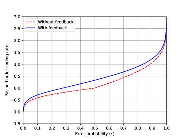
Figure 1: Second order coding rate with and without feedback for the channel in (5) with $p=0.8$. For this channel, the lower bound in Theorem 13 and the upper bound in Theorem 4 coincide, determining the second-order coding rate with feedback.

for the channel in (5) with $p=0.8$ and $q$ selected to satisfy (4). Note that the range of $\varepsilon$ over which one can approach the capacity from above, i.e., for which the second-order coding rate is positive, is enlarged by the presence of feedback. The right-hand-side of (13) is easily verified to exceed $\sqrt{V_{\varepsilon}}\Phi^{-1}(\varepsilon)$ for all $\varepsilon$ if the channel is compound-dispersion (i.e., $\beta<1$). The next result shows that if the channel is not compound-dispersion then feedback does not improve the second-order coding rate.

Theorem 3 (Feedback does not improve the second-order coding rate for simple-dispersion channels).

For any $W\in\mathcal{P}(\mathcal{Y}|\mathcal{X})$ with $0<V_{\text{min}}=V_{\text{max}}$ (i.e., simple-dispersion) and any $\varepsilon\in(0,1)$,

$$\limsup_{n\to\infty}\frac{\log M_{\textnormal{fb}}^{\ast}(n,\varepsilon)-nC}{\sqrt{n}}\leq\sqrt{V_{\min}}\Phi^{-1}\left(\varepsilon\right)=\sqrt{V_{\varepsilon}}\Phi^{-1}\left(\varepsilon\right)$$

Proof:

Please see Section V. ∎

The proof of Theorem 3 uses a method of making feedback codes “constant-composition,” which is inspired by Fong and Tan’s work on parallel Gaussian channels [12]. Fong and Tan have also noted that their techniques can be applied to DMCs to obtain something like Theorem 3 [21].

If the channel is compound dispersion, then feedback improves the second-order coding rate, and Theorem 13 (along with (9)) provides a lower bound on the size of the improvement. The next theorem provides a comparable upper bound.

Theorem 4 (Impossibility for compound-dispersion channels).

Consider any $W\in{\cal P}({\cal Y}|{\cal X})$ with $0<\nu_{\text{min}}$ and let $\lambda\mathrel{\mathop{:}}=\sqrt{\nu_{\text{min}}/\nu_{\text{max}}}$. Then

$$\limsup_{n\to\infty}\frac{\log M^{\ast}_{\textnormal{fb}}(n,\varepsilon)-nC}{\sqrt{n}}\leq\begin{cases}\sqrt{\nu_{\text{min}}}\Phi^{-1}\left(\frac{1}{2\lambda}\varepsilon(1+\lambda)\right),&\varepsilon\in\left(0,\frac{\lambda}{1+\lambda}\right],\\ \sqrt{\nu_{\text{max}}}\Phi^{-1}\left(\frac{1}{2}[\varepsilon(1+\lambda)+(1-\lambda)]\right),&\varepsilon\in\left(\frac{\lambda}{1+\lambda},1\right).\end{cases}$$ (14)

Proof:

Please see Section VI. ∎

The upper bound in Theorem 4 equals the achievability result in Theorem 13 but with $\nu_{\text{min}}$ and $\nu_{\text{max}}$ replacing $V_{\min}$ and $V_{\max}$, respectively. Thus the two results are similar in spirit. Both, in fact, use McNamara’s scheme in (1). However, the range of values that the diffusion coefficient can assume is larger for the upper bound ($[\sqrt{\nu_{\text{min}}},\sqrt{\nu_{\text{max}}}]$) than for the lower bound ($[\sqrt{V_{\min}},\sqrt{V_{\max}}]$). For the channel in (5), $\nu_{\text{max}}=V_{\max}$ and $\nu_{\text{min}}=V_{\min}$, so the upper and lower bound coincide and the second-order coding rate with feedback is determined (and is depicted in Fig. 1). The two bounds do not coincide in general, however.

Finally, we consider very noisy channels (VNCs). For our purposes, a very noisy channel is one of the form

$$W_{\zeta}(y|x)=\Gamma(y)\left(1+\zeta\lambda(x,y)\right),$$ (15)

where $\Gamma$ is a probability distribution on the output alphabet $\mathcal{Y}$ such that $\Gamma(y)>0$ for all $y$, $\lambda(x,y)$ satisfies

$$\sum_{y\in\mathcal{Y}}\Gamma(y)\lambda(x,y)=0$$ (16)

for all $x\in\mathcal{X}$, and $\zeta$ is infinitesimally small. In the very noisy limit, i.e., as $\zeta$ tends to zero, $V_{\min}$ and $V_{\max}$ converge together and the channel behaves as one with simple dispersion. In light of Theorem 3, one therefore expects feedback not to improve the second-order coding rate in the very noisy limit. Since $V_{\min}$ and $V_{\max}$ are only equal in the limit (when suitably scaled), the result does not follow from Theorem 3, however. Since $\sqrt{\nu_{\text{min}}}$ and $\sqrt{\nu_{\text{max}}}$ do not necessarily converge together, the result does not follow from Theorem 4 either.

Theorem 5 (Feedback does not improve the second-order coding rate in the very noisy limit).

Consider a channel family $W_{\zeta}\in{\cal P}({\cal Y}|{\cal X})$ of the form $W_{\zeta}(y|x)=\Gamma(y)\left(1+\zeta\lambda(x,y)\right),$ with $\Gamma\in{\cal P}({\cal Y})$. Let $C_{\zeta}$, $V_{\text{min},\zeta}$, $V_{\text{max},\zeta}$, and $\log M^{\ast}_{\textnormal{fb},\zeta}(n,\varepsilon)$ denote $C$, $V_{\min}$, $V_{\max}$, and $M^{\ast}_{\textnormal{fb}}(n,\varepsilon)$, respectively, for the channel $W_{\zeta}\in{\cal P}({\cal Y}|{\cal X})$. If

$$\max_{P\in\mathcal{P}(\mathcal{X})}\frac{1}{2}\sum_{y\in\mathcal{Y}}\Gamma(y)\Bigg{(}\left.\sum_{x\in\mathcal{X}}P(x)\lambda^{2}(x,y)-\left(\sum_{x\in\mathcal{X}}P(x)\lambda(x,y)\right)^{2}\right)>0,$$

which ensures that $C_{\zeta}>0$ for all sufficiently small $\zeta$, then

$$\limsup_{\zeta\to 0}\limsup_{n\to\infty}\frac{\log M^{\ast}_{\textnormal{fb},\zeta}(n,\varepsilon)-nC_{\zeta}}{\sqrt{nV_{\text{min},\zeta}}}\leq\Phi^{-1}(\varepsilon), \quad\varepsilon\in\left(0,\frac{1}{2}\right]$$

$$\limsup_{\zeta\to 0}\limsup_{n\to\infty}\frac{\log M^{\ast}_{\textnormal{fb},\zeta}(n,\varepsilon)-nC_{\zeta}}{\sqrt{nV_{\text{max},\zeta}}}\leq\Phi^{-1}(\varepsilon), \quad\varepsilon\in\left(\frac{1}{2},1\right).$$

Proof:

Please see Section VII. ∎

One can also show that feedback does not improve the high-rate error exponent or moderate deviations performance of VNCs [22]. Note that very noisy channels are unusual in that their reliability function is known at all rates [18, 23].

The next five sections contain the proofs of Theorems 1 through 5, respectively.

III Proof of Theorem 1

Note that $f(\cdot)$ is continuous on $[1,\infty)$ and $f(1)<0$. Hence there exists $1<\alpha<1/(2\varepsilon)$ with $f(\alpha)<0$ and we fix any such $\alpha$ in what follows. Define

$$\nu=\sqrt{2}\Phi^{-1}(\alpha\varepsilon)<0.$$ (17)

We shall use Lemma 14 in the Appendix. Note that we only require that (130) holds with the limit superior taken along the even integers. Accordingly, suppose that $n$ is even. Let $Q_{\max}$ denote a distribution on $\mathcal{P}(\mathcal{X})$ that attains $V_{\max}$, and define $Q_{\min}$ similarly. Select the controller $F$ as follows

$$F(x^{k},y^{k})=\begin{cases}Q_{\min}&\text{if $k\leq n/2$}\\ Q_{\min}&\text{if $k>n/2$ and $\log\frac{W(y^{n/2}|x^{n/2})}{q^{*}(y^{n/2})}>\frac{nC}{2}+\nu\sqrt{\frac{nV_{\min}}{2}}$}\\ Q_{\max}&\text{if $k>n/2$ and $\log\frac{W(y^{n/2}|x^{n/2})}{q^{*}(y^{n/2})}\leq\frac{nC}{2}+\nu\sqrt{\frac{nV_{\min}}{2}}$}.\end{cases}$$ (18)

Note that $FW=q^{*}\times q^{*}\times\cdots q^{*}$. For convenience we define

$$\Gamma_{n}=(F\circ W)\left(\sum_{k=1}^{n}\log\frac{W(Y_{k}|X_{k})}{q^{*}(Y_{k})}\leq nC+\sqrt{nV_{\min}}\Phi^{-1}(\alpha\varepsilon)\right).$$ (19)

Let $\underline{G}_{n}$ denote the CDF of $\frac{1}{\sqrt{(n/2)V_{\min}}}\sum_{i=1}^{n/2}\left[\log\frac{W(Y_{i}|X_{i})}{q^{\ast}(Y_{i})}-C\right]$ when $\left\{\log\frac{W(Y_{i}|X_{i})}{q^{\ast}(Y_{i})}\right\}_{i=1}^{n/2}$ are i.i.d. with distribution $Q_{\min}\circ W$. Similarly, let $\overline{G}_{n}$ denote the distribution of $\frac{1}{\sqrt{(n/2)V_{\min}}}\sum_{i=1}^{n/2}\left[\log\frac{W(Y_{i}|X_{i})}{q^{\ast}(Y_{i})}-C\right]$ when $\left\{\log\frac{W(Y_{i}|X_{i})}{q^{\ast}(Y_{i})}\right\}_{i=1}^{n/2}$ are i.i.d. with distribution $Q_{\max}\circ W$. We have

$$\Gamma_{n} =\int\limits_{\nu}^{\infty}\underline{G}_{n}\left(\nu-x\right)d\underline{G}_{n}(x)+\int\limits_{-\infty}^{\nu}\overline{G}_{n}\left(\nu-x\right)d\underline{G}_{n}(x)$$

$$=\underline{G}_{2n}\left(\Phi^{-1}(\alpha\varepsilon)\right)-\int\limits_{-\infty}^{\nu}\left[\underline{G}_{n}\left(\nu-x\right)-\overline{G}_{n}\left(\nu-x\right)\right]d\underline{G}_{n}(x).$$ (20)

From the Berry-Esseen theorem [25, 26], along with a first-order Taylor series approximation, we deduce that

$$\underline{G}_{2n}\left(\Phi^{-1}(\alpha\varepsilon)\right)\leq\alpha\varepsilon+\frac{\underline{\kappa}}{2\sqrt{n}},$$ (21)

where $\underline{\kappa}\mathrel{\mathop{:}}=\mathbb{E}_{Q_{\min}\circ W}\left[\left|\log W(Y|X)/q^{\ast}(Y)-C\right|^{3}\right]/V_{\min}^{3/2}+1$. Another application of the Berry-Esseen theorem implies that for any $x\in\mathbb{R}$,

$$\left|\underline{G}_{n}\left(\nu-x\right)-\Phi\left(\nu-x\right)\right|\leq\frac{\underline{\kappa}}{\sqrt{2n}},$$ (22)

$$\left|\overline{G}_{n}\left(\nu-x\right)-\Phi\left(\beta\left[\nu-x\right]\right)\right|\leq\frac{\overline{\kappa}}{\sqrt{2n}},$$ (23)

where $\overline{\kappa}\mathrel{\mathop{:}}=\mathbb{E}_{Q_{\max}\circ W}\left[\left|\log W(Y|X)/q^{\ast}(Y)-C\right|^{3}\right]/V_{\max}^{3/2}+1$. Equations (22) and (23) imply that

$$\int\limits_{-\infty}^{\nu}\left[\underline{G}_{n}(\nu-x)-\overline{G}_{n}(\nu-x)\right]d\underline{G}_{n}(x) \geq\int\limits_{-\infty}^{\nu}\left[\Phi(\nu-x)-\Phi\left(\beta\left[\nu-x\right]\right)\right]d\underline{G}_{n}(x)-\frac{\underline{\kappa}+\overline{\kappa}}{\sqrt{2n}}$$ (24)

$$=\int\limits_{-\infty}^{\nu}\underline{G}_{n}(x)\left[\phi(\nu-x)-\beta\phi\left(\beta\left[\nu-x\right]\right)\right]dx-\frac{\underline{\kappa}+\overline{\kappa}}{\sqrt{2n}}$$ (25)

$$\geq\int\limits_{-\infty}^{\nu}\Phi(x)\left[\phi(\nu-x)-\beta\phi\left(\beta\left[\nu-x\right]\right)\right]dx-\frac{3\underline{\kappa}+\overline{\kappa}}{\sqrt{2n}}$$ (26)

$$=\int\limits_{-\infty}^{\nu}\phi(x)\left[\Phi(\nu-x)-\Phi(\beta[\nu-x])\right]dx-\frac{3\underline{\kappa}+\overline{\kappa}}{\sqrt{2n}},$$ (27)

where (25) and (27) follow from integration by parts and (26) follows from the Berry-Esseen theorem. We continue as follows

$$\int\limits_{-\infty}^{\nu}\phi(x)\left[\Phi(\nu-x)-\Phi(\beta[\nu-x])\right]dx =\int\limits_{0}^{\infty}\phi(\nu-z)\int\limits_{\beta z}^{z}\phi(\zeta)d\zeta dz$$ (28)

$$\geq(1-\beta)\int\limits_{0}^{\infty}\phi(\nu-z)z\phi(z)dz$$ (29)

$$\geq(1-\beta)\phi(2\nu)\int\limits_{0}^{-\nu}z\phi(z)dz$$ (30)

$$=(1-\beta)\phi(2\nu)\left(\frac{1}{\sqrt{2\pi}}-\phi(\nu)\right).$$ (31)

By plugging (31) into (27), and recalling (20) and (21), we deduce that

$$\Gamma_{n}\leq f(\alpha)+\varepsilon+\frac{4\underline{\kappa}+\overline{\kappa}}{\sqrt{2n}}.$$ (32)

Thus for all sufficiently large (and even) $n$, we have

$$\Gamma_{n}<\varepsilon.$$ (33)

So by Lemma 14,

$$\liminf_{n\rightarrow\infty}\frac{\log M^{\ast}_{\textnormal{fb}}(n,\varepsilon)-nC}{\sqrt{n}}\geq\sqrt{V_{\min}}\Phi^{-1}(\alpha\varepsilon).$$ (34)

∎

Remark 2.

Although Theorem 1 uses feedback only at a single epoch, it still provides a strict improvement over the best non-feedback code. It is possible to prove a version of Theorem 1 for large $\varepsilon$, but we shall not pursue this here because our aim with Theorem 1 is only to elucidate the idea behind timid/bold coding while avoiding the diffusion machinery used in our main achievability result, Theorem 13. Theorem 13 takes timid/bold coding to its natural limit by allowing the encoder to switch between timid and bold signaling schemes after each time-step.   $\Diamond$

IV Proof of Theorem 13

Following Øksendal (e.g., [27, Def. 7.1.1]), we define a one-dimensional, time-homogeneous Itô diffusion as follows.

Definition 3 (Itô diffusion).

A time-homogeneous Itô diffusion is a stochastic process $\mathbf{X}$ satisfying a stochastic differential equation of the form

$$X_{t}=x_{0}+\int\limits_{0}^{t}b(X_{s})\,ds+\int\limits_{0}^{t}\sigma(X_{s})\,dB_{s},$$ (35)

for some one-dimensional Brownian Motion $\mathbf{B}$ defined on the same sample space, where $b\colon\mathbb{R}\to\mathbb{R}$ and $\sigma\colon\mathbb{R}\to\mathbb{R}$ are measurable functions that satisfy

$$|b(x)-b(y)|+|\sigma(x)-\sigma(y)|\leq D|x-y|,\,\forall\,x,y\in\mathbb{R},$$ (36)

for some constant $D\in\mathbb{R}^{+}$.

Remark 3.

Since (36) ensures that the conditions in [27, Theorem 5.2.1] are satisfied, (35) has a unique solution.

IV-A A convergence result

Let $\{Z_{i,k}\}_{k=1}^{\infty}$, $i\in\{0,1\}$ denote i.i.d. sequences of bounded random variables, which are also independent of each other, such that for any $k\in\mathbb{Z}^{+}$,

$$\mathbb{E}[Z_{0,k}]=\mathbb{E}[Z_{1,k}] =0,$$ (37)

$$\mathbb{E}[Z_{1,k}^{2}] =1,$$ (38)

$$\mathbb{E}[Z_{0,k}^{2}] =\beta^{2},$$ (39)

with $\beta\in(0,1)$. Given any $\delta\in(0,1]$ and $x\in[0,\delta]$, define

$$\alpha_{\delta}(x)\mathrel{\mathop{:}}=\frac{1}{1-\beta^{2}}\left(\left[1-x\left(\frac{1-\beta}{\delta}\right)\right]^{2}-\beta^{2}\right).$$ (40)

Via direct computation, one can verify that

$$\alpha_{\delta}(x)\in[0,1],$$ (41)

for the given range of $\delta$ and $x$. Let $\mu_{i}$ denote the law of $Z_{i,1}$ for $i\in\{0,1\}$. Define the probability measure

$$\mu_{\delta,x}\mathrel{\mathop{:}}=(1-\alpha_{\delta}(x))\mu_{0}+\alpha_{\delta}(x)\mu_{1}.$$ (42)

For any $\varepsilon\in(0,1)$, define

$$s(\varepsilon)\mathrel{\mathop{:}}=\begin{cases}-\beta\Phi^{-1}\left(\frac{1}{2\beta}\varepsilon(1+\beta)\right),&\varepsilon\in(0,\frac{\beta}{1+\beta}],\\ -\Phi^{-1}\left(\frac{1}{2}[\varepsilon(1+\beta)+(1-\beta)]\right),&\varepsilon\in(\frac{\beta}{1+\beta},1).\end{cases}$$ (43)

For any $\varepsilon\in(0,1)$ and $n\in\mathbb{Z}^{+}$,

$$S_{0}^{\delta,\varepsilon,n} \mathrel{\mathop{:}}=s(\varepsilon)\sqrt{n},$$ (44)

$$S_{k+1}^{\delta,\varepsilon,n} \mathrel{\mathop{:}}=S_{k}^{\delta,\varepsilon,n}+{\mathbf{1}}\left\{S_{k}^{\delta,\varepsilon,n}\leq 0\right\}Z_{1,k+1}+{\mathbf{1}}\left\{S_{k}^{\delta,\varepsilon,n}>\delta\sqrt{n}\right\}Z_{0,k+1}+{\mathbf{1}}\left\{0<S_{k}^{\delta,\varepsilon,n}\leq\delta\sqrt{n}\right\}Z_{2,k+1},$$ (45)

for all $k\in\mathbb{Z}^{+}$, where $Z_{2,k+1}$ has distribution $\mu_{\delta,S_{k}^{\delta,\varepsilon,n}/\sqrt{n}}$ and is independent of $\{Z_{i,j}\}_{j=1}^{\infty}$, $i\in\{0,1\}$ and $\{Z_{2,j}\}_{j=1}^{k}.$

Proposition 1.

Consider any $\varepsilon\in(0,1)$. For any $\kappa\in\mathbb{R}^{+}$, there exist $\delta_{\textnormal{o}}\in(0,1)$ and $n_{\textnormal{o}}\in\mathbb{Z}^{+}$ such that for all $n\geq n_{\textnormal{o}}$,

$$\Pr\left(\frac{1}{\sqrt{n}}S_{n}^{\delta_{\textnormal{o}},\varepsilon,n}\leq 0\right)\leq\varepsilon+\kappa.$$ (46)

Proof:

Similar to [28, p. 43], we interpolate the discrete-time Markov process defined in (44) and (45) as follows

$$\xi^{\varepsilon,\delta,n}_{t}\mathrel{\mathop{:}}=\frac{1}{\sqrt{n}}S^{\delta,\varepsilon,n}_{[nt]},$$ (47)

for any $t\in\mathbb{R}_{+}$, where $[nt]$ denotes the integer part of $nt$. We prove the claim by investigating the limiting behavior of $\xi^{\varepsilon,\delta,n}_{t}$ as $\delta\to 0$ and $n\to\infty$. To this end, we use several stochastic processes, which are defined next.

For any $\delta\in(0,1]$, define $\sigma_{\delta}:\mathbb{R}\to\mathbb{R}$ as

$$\sigma_{\delta}(x)\mathrel{\mathop{:}}=\begin{cases}1,&x\leq 0,\\ 1-x\left(\frac{1-\beta}{\delta}\right),&0\leq x\leq\delta,\\ \beta,&x\geq\delta.\end{cases}$$ (48)

Clearly, $\sigma_{\delta}(\cdot)$ is Lipschitz continuous, positive and bounded. For any $\varepsilon\in(0,1)$, we use (48) to define an Itô diffusion $\xi^{\varepsilon,\delta}_{t}$ that is the solution of the following stochastic differential equation:

$$\xi^{\varepsilon,\delta}_{t}=\xi^{\varepsilon,\delta}_{0}+\int\limits_{0}^{t}\sigma_{\delta}(\xi^{\varepsilon,\delta}_{s})\,dB_{s},$$ (49)

with $\xi^{\varepsilon,\delta}_{0}\mathrel{\mathop{:}}=s(\varepsilon)$. Further, define $\bar{\sigma}:\mathbb{R}\to\mathbb{R}$ with

$$\bar{\sigma}(x)\mathrel{\mathop{:}}={\mathbf{1}}\{x\leq 0\}+\beta{\mathbf{1}}\{x>0\},$$ (50)

and let $\xi^{\varepsilon,0}_{t}$ be the solution of the following stochastic differential equation

$$\xi^{\varepsilon,0}_{t}=\xi^{\varepsilon,0}_{0}+\int\limits_{0}^{t}\bar{\sigma}(\xi^{\varepsilon,0}_{s})\,dB_{s},$$ (51)

with $\xi^{\varepsilon,0}_{0}\mathrel{\mathop{:}}=s(\varepsilon)$. Existence of a (weak) solution of (51) can be verified by using [29, Theorem 23.1]. Further, an expression for the transition probabilities of the Markov process $\xi^{\varepsilon,0}_{t}$, denoted by $P_{t}(x,y)$, is known [30],

$$P_{t}(x,y)=\frac{1}{\sqrt{2\pi t}}\begin{cases}\frac{1}{\beta}\exp\left(-(x-y)^{2}/2\beta^{2}t\right)-\frac{(\beta-1)}{\beta(\beta+1)}\exp\left({-(x+y)^{2}/2\beta^{2}t}\right),&(x,y)\in\mathbb{R}^{+}\times\mathbb{R}^{+},\\ \frac{2\beta}{(\beta+1)}\exp\left({-(x-\beta y)^{2}/2\beta^{2}t}\right),&(x,y)\in\mathbb{R}^{+}\times\mathbb{R}^{-},\\ \frac{2}{\beta(\beta+1)}\exp\left({-(\beta x-y)^{2}/2\beta^{2}t}\right),&(x,y)\in\mathbb{R}^{-}\times\mathbb{R}^{+},\\ \exp\left({-(x-y)^{2}/2t}\right)+\frac{(\beta-1)}{(\beta+1)}\exp\left({-(x+y)^{2}/2t}\right),&(x,y)\in\mathbb{R}^{-}\times\mathbb{R}^{-}.\end{cases}$$ (52)

In Lemmas 53 and 2 to follow, the mode of convergence is the weak convergence of probability measures in the space of right-continuous functions with left limits defined on $[0,1]$, i.e., $D[0,1]$, endowed with the Skorohod topology (e.g., [31, Section 12]).

Lemma 1.

$$\boldsymbol{\xi}^{\varepsilon,\delta}\xrightarrow{w.}\boldsymbol{\xi}^{\varepsilon,0},\textnormal{ as }\delta\to 0.$$ (53)

Proof:

The claim follows from a convergence result due to Kulinich [32, Theorem 2]. To verify the conditions of this theorem for our case, we note that the function $f_{\delta}$ in [32, p. 856] can be taken to be $f_{\delta}(x)=x$, either by direct calculation or by noticing the fact that the Itô diffusion $\xi^{\varepsilon,\delta}_{t}$ is in its natural scale. The condition regarding $f^{\prime}_{\delta}(\cdot)\sigma_{\delta}(\cdot)$ is satisfied, since

$$\beta\leq f^{\prime}_{\delta}(x)\sigma_{\delta}(x)\leq 1,$$ (54)

for all $\delta\in(0,1]$ and $x\in\mathbb{R}$. Further, the condition

$$\lim_{K\to\infty}\lim_{\delta\to 0}\Pr(|f_{\delta}(\xi^{\varepsilon,\delta}_{0})|>K)=0,$$ (55)

is also clearly satisfied since

$$f_{\delta}(\xi^{\varepsilon,\delta}_{0})=s(\varepsilon)\in\mathbb{R}.$$ (56)

Finally, the condition regarding the function $G_{\delta}$, which is defined in [32, p. 857], can be verified to hold for our case, since for any $x\in\mathbb{R}$, we have

$$\lim_{\delta\to 0}G_{\delta}(x) =\lim_{\delta\to 0}\int\limits_{0}^{x}\frac{\,du}{\sigma^{2}_{\delta}(u)}$$ (57)

$$=\frac{x}{\bar{\sigma}^{2}(x)},$$ (58)

via direct calculation. Hence, we can apply [32, Theorem 2] to deduce the assertion, since the generalized diffusion used in this theorem, which is defined in [32, Eq. (3)], reduces to $\xi^{0}_{t}$ in our case. ∎

Lemma 2.

For any $\delta\in(0,1]$,

$$\boldsymbol{\xi}^{\varepsilon,\delta,n}\xrightarrow{w.}\boldsymbol{\xi}^{\varepsilon,\delta}\textnormal{ as }n\to\infty.$$ (59)

Proof:

The claim follows from a convergence result of Kushner [28, Theorem 1]. Specifically, we apply this theorem with the Markov chain

$$\left\{\frac{1}{\sqrt{n}}S_{k}^{\delta,\varepsilon,n}\right\}_{k=0}^{\infty},$$ (60)

$\mathcal{F}_{k,n}$ denoting the sigma-algebra generated by $\frac{S_{i}^{\delta,\varepsilon,n}}{\sqrt{n}}$ for all $i\leq k$, and the sequence of positive real numbers $\delta t_{i}^{n}=\frac{1}{n}$. The definition of $S_{k}^{\delta,\varepsilon,n}$, along with (48) and elementary algebra, ensures that for any $n\in\mathbb{Z}^{+}$, we have

$$\mathbb{E}\left[\left(S_{k+1}^{\delta,\varepsilon,n}-S_{k}^{\delta,\varepsilon,n}\right)^{2}\bigg{|}\mathcal{F}_{k,n}\right]=\sigma^{2}_{\delta}\left(\frac{S_{k}^{\delta,\varepsilon,n}}{\sqrt{n}}\right)\textnormal{ (a.s.)},$$ (61)

for all $t\in\mathbb{R}_{+}$ and $k\in\{0,\ldots,[nt]\}$, and hence the condition in [28, Eq. (1)] is satisfied. The proof will be complete if we can verify that the six assumptions of Kushner [28, pg. 42] are satisfied for our case. Indeed, except (A4) and (A6), these assumptions trivially hold with the aforementioned choices. (A6) is evidently true since $\xi^{\varepsilon,\delta}_{t}$ is the unique (strong) solution of (49), whereas (A6) only requires (49) to possess a unique weak solution (e.g., [27, Chapter 5.3]). To verify (A4), let $K\in\mathbb{R}^{+}$ be a constant such that

$$\max\{|Z_{0,1}|,|Z_{1,1}|\}\leq K\textnormal{ (a.s.)},$$ (62)

whose existence is ensured by the boundedness of the random variables. From the definition of $S_{k}^{\delta,\varepsilon,n}$, one can verify that for any $t\in\mathbb{R}^{+}$,

$$0 \leq\mathbb{E}\left[\sum_{k=0}^{[nt]}\left|\frac{S_{k+1}^{\delta,\varepsilon,n}-S_{k}^{\delta,\varepsilon,n}}{\sqrt{n}}\right|^{3}\right]$$ (63)

$$\leq\frac{1}{n^{3/2}}K^{3}([nt]+1)\to 0,\textnormal{ as }n\to\infty.$$ (64)

Evidently, (64) implies (A4) and hence we can apply [28, Theorem 1] to infer the assertion. ∎

In order to conclude the proof, it suffices to note that

$$\lim_{\delta\to 0}\Pr(\xi^{\varepsilon,\delta}_{1}\leq 0) =\Pr(\xi^{\varepsilon,0}_{1}\leq 0),$$ (65)

$$\lim_{n\to\infty}\Pr(\xi^{\varepsilon,\delta,n}_{1}\leq 0) =\Pr(\xi^{\varepsilon,\delta}_{1}\leq 0),\,\forall\,\delta\in(0,1],$$ (66)

$$\Pr(\xi^{\varepsilon,0}_{1}\leq 0) =\varepsilon,$$ (67)

where (65) and (66) follow from Lemmas 53 and 2, respectively, along with [31, Theorem 12.5], whereas (67) follows from an elementary calculation by using (52). ∎

IV-B Proof of Theorem 13

Fix any $\varepsilon\in(0,1)$. If $\beta=1$ then the result is implied by (9). Otherwise, assume that

$$\beta=\sqrt{\frac{V_{\min}}{V_{\max}}}\in(0,1).$$ (68)

Choose some $0<\kappa<\frac{\varepsilon}{2}$ that also satisfies

$$\kappa\leq\frac{\left[\varepsilon-\frac{\beta}{1+\beta}\right]}{4}$$ (69)

if $\varepsilon>\frac{\beta}{1+\beta}$. Define $r:(0,1)\mapsto\mathbb{R}$ as

$$r(a)\mathrel{\mathop{:}}=\begin{cases}\sqrt{V_{\min}}\Phi^{-1}\left(\frac{a(1+\beta)}{2\beta}\right),&0<a\leq\frac{\beta}{1+\beta},\\ \sqrt{V_{\max}}\Phi^{-1}\left(\frac{a(1+\beta)+(1-\beta)}{2}\right),&\frac{\beta}{1+\beta}<a<1.\end{cases}$$ (70)

Using $r(\cdot)$, define

$$R_{n}(\cdot)\mathrel{\mathop{:}}=C+\frac{r(\cdot)}{\sqrt{n}}.$$ (71)

Again we shall use Lemma 14 in the Appendix. To this end, define the controller $F_{\ell}$ via

$$F_{\ell}(x^{k-1},y^{k-1})=\begin{cases}Q_{\max},&\sum\limits_{j=1}^{k-1}\left[\log\frac{W(y_{j}|x_{j})}{q^{\ast}(y_{j})}-C\right]\leq\sqrt{n}r(\varepsilon-\kappa),\\ Q_{\min},&\sum\limits_{j=1}^{k-1}\left[\log\frac{W(y_{j}|x_{j})}{q^{\ast}(y_{j})}-C\right]>\sqrt{n}r(\varepsilon-\kappa)+\frac{1}{\ell}\sqrt{nV_{\max}},\\ \alpha_{\ell,k}Q_{\max}+(1-\alpha_{\ell,k})Q_{\min},&\textnormal{else},\end{cases}$$ (72)

where

$$\alpha_{\ell,k}\mathrel{\mathop{:}}=\alpha_{1/\ell}\left(-\frac{r(\varepsilon-\kappa)}{\sqrt{V_{\max}}}+\frac{1}{\sqrt{nV_{\max}}}\sum_{j=1}^{k-1}\left[\log\frac{W(y_{j}|x_{j})}{q^{\ast}(y_{j})}-C\right]\right),$$ (73)

by using the function defined in (40) and with a slight abuse of notation, we let

$$\sum_{j=1}^{0}\left[\log\frac{W(y_{j}|x_{j})}{q^{\ast}(y_{j})}-C\right]=0.$$ (74)

By Proposition 46, there exists $\ell_{0}$ in $\mathbb{Z}^{+}$ and $n_{0}$ in $\mathbb{Z}^{+}$ such that if $n\geq n_{0}$ and $\ell\geq\ell_{0}$,

$$(F_{\ell}\circ W)\left(\frac{1}{\sqrt{n}}\sum_{k=1}^{n}\left(\log\frac{W(Y_{k}|X_{k})}{q^{*}(Y_{k})}-C\right)-r(\varepsilon-\kappa)\leq 0\right)\leq\varepsilon-\frac{\kappa}{2}.$$ (75)

Lemma 14 then implies that

$$\liminf_{n\rightarrow\infty}\frac{\log M_{\textnormal{fb}}^{\ast}(n,\varepsilon)-nC}{\sqrt{n}}\geq r(\varepsilon-\kappa).$$ (76)

Since $r(\cdot)$ is continuous and $\kappa>0$ is arbitrary, the result follows. ∎

V Proof of Theorem 3

Our approach will be to show that, for the code to have rate approaching capacity and error probability diminishing to zero, then, with high probability, the empirical distribution of $\mathbf{X}^{n}$ needs to be near the set of capacity-achieving input distributions. Since $V_{\min}=V_{\max}$, if the empirical distribution of $\mathbf{X}^{n}$ is nearly capacity-achieving, then the sum of the conditional variances of $\mathfrak{i}^{*}(X_{k},Y_{k})$ given the past is close to $nV_{\min}$ a.s., and a martingale central limit theorem[33] can be applied. We begin with a few definitions needed for the reduction to codes with empirically-capacity-achieving $\mathbf{X}^{n}$.

Definition 4.

The type of a sequence $\mathbf{x}^{n}$ is the distribution $P_{\mathbf{x}^{n}}$ on $\mathcal{X}$ defined as

$$P_{\mathbf{x}^{n}}(a)\mathrel{\mathop{:}}=\frac{1}{n}\sum_{k=1}^{n}\mathbf{1}\{x_{k}=a\}.$$

Definition 5.

For a sequence $\mathbf{x}^{n}\in\mathcal{X}^{n}$,

$$\phi_{W}(\mathbf{x}^{n})\mathrel{\mathop{:}}=\inf_{P\in\Pi^{\ast}_{W}}d_{\text{TV}}(P,P_{\mathbf{x}^{n}}),$$

where $d_{\text{TV}}(P,Q)$ denotes the total variation distance between distributions $P$ and $Q$.

Definition 6.

Let $\mathcal{T}^{n}$ denote the set of all probability distributions on $\mathcal{X}$ that are types of some length-$n$ sequence, and define

$$\mathcal{T}^{n}_{\gamma}\mathrel{\mathop{:}}=\left\{T\in\mathcal{T}^{n},\inf_{P\in\Pi^{\ast}_{W}}d_{\text{TV}}(P,T)>\gamma\right\},$$

$$\mathcal{T}^{c,n}_{\gamma}\mathrel{\mathop{:}}=\left\{T\in\mathcal{T}^{n},\inf_{P\in\Pi^{\ast}_{W}}d_{\text{TV}}(P,T)\leq\gamma\right\}.$$

Let $\mathbf{f}(m,\mathbf{y}^{i})\mathrel{\mathop{:}}=[f(m,\mathbf{y}^{0}),f(m,\mathbf{y}^{1}),\dots,f(m,\mathbf{y}^{i})]\in\mathcal{X}^{i+1}$ with the convention that both $\mathbf{y}^{0}$ and $\mathbf{f}(m,\mathbf{y}^{i})$ for $i\leq-1$ are empty strings.

Definition 7.

If $Q$ is a probability distribution on $\mathcal{X}$ and $A\subset\mathcal{X}$ is such that $Q(A)>0$, then $Q|_{A}$ is the probability measure

$$Q_{A}(x)=\begin{cases}\frac{Q(x)}{Q(A)}&\text{if $x\in A$}\\ 0&\text{otherwise}.\end{cases}$$ (77)

Definition 8.

Given a controller $F:(\mathcal{X}\times\mathcal{Y})^{*}\mapsto\mathcal{P}(\mathcal{X})$, the $(*,\gamma)$-modified controller $\tilde{F}$ is defined as follows. For $k<n$ and $x^{k}\in\mathcal{X}^{k}$, let

$$\mathcal{X}_{x^{k}}=\{x:(x^{k},x)\ \text{is a prefix of some $x^{n}\in\mathcal{T}^{c,n}_{\gamma}$}\}.$$ (78)

Fix some $x_{0}\in\mathcal{X}$ arbitrarily. Let $\tilde{F}(x^{k},y^{k})$ be a point-mass on $x_{0}$ if either $k\geq n$ or $k<n$ but $F(x^{k},y^{k})(\mathcal{X}_{x^{k}})=0$ (note that the latter includes the case in which $\mathcal{X}_{x^{k}}$ is empty). Otherwise, let

$$\tilde{F}(x^{k},y^{k})=F(x^{k},y^{k})|_{\mathcal{X}_{x^{k}}}.$$ (79)

Definition 9.

Given a controller $F:(\mathcal{X}\times\mathcal{Y})^{*}\mapsto\mathcal{P}(\mathcal{X})$, the $(T,\gamma)$-modified controller is defined as in the previous definition but with the type $T$ in place of $\mathcal{T}^{c,n}_{\gamma}$.

Lemma 15 in the Appendix states for any $\rho_{n}>0$

$$\log M_{\textnormal{fb}}^{\ast}(n,\varepsilon)\leq\sup_{F}\inf_{q}\left(\log\rho_{n}-\log\left(\left[1-\varepsilon-F\circ W\left(\log\frac{\prod_{k=1}^{n}W(Y_{k}|X_{k})}{q(\mathbf{Y}^{n})}\geq\log\rho_{n}\right)\right]^{+}\right)\right),$$ (80)

where $F$ is a controller: $F:(\mathcal{X}\times\mathcal{Y})^{\ast}\rightarrow\mathcal{P}(\mathcal{X})$. Let $P$ denote the distribution $F\circ W$. We will choose

$$q(\mathbf{y}^{n})=\frac{1}{2}\prod_{k=1}^{n}q^{\ast}(y_{k})+\frac{1}{2|\mathcal{T}^{n}_{\gamma}|}\sum_{T\in\mathcal{T}^{n}_{\gamma}}\prod_{k=1}^{n}q_{T}(y_{k}),$$ (81)

where

$$q_{T}(y)\mathrel{\mathop{:}}=\sum_{x\in\mathcal{X}}T(x)W(y|x).$$

This choice is inspired by an analogous choice by Fong and Tan [12, (37)], who in turn credit Hayashi [34].

Let $K_{W}\mathrel{\mathop{:}}=\max\left(2|\mathcal{X}|\nu_{\text{max}},\frac{8|\mathcal{X}|\nu_{\text{max}}}{V_{\min}}\right)$ and $\chi_{W}$ denote the constant in [33, Corollary to Theorem 2] when $\gamma$ in that result is taken to be $2\mathfrak{i}_{\text{max}}$ here. Fix $0<\gamma\leq\frac{V_{\min}}{4|\mathcal{X}|\nu_{\text{max}}}$, and define

$$\delta_{n} \mathrel{\mathop{:}}=\chi_{W}\cdot\left(\frac{\log n}{\sqrt{n}(V_{\min}-\gamma K_{W})^{3/2}}+\sqrt{\gamma K_{W}}\right),$$

$$r_{n} \mathrel{\mathop{:}}=\begin{cases}\sqrt{V_{\min}-\gamma K_{W}}\Phi^{-1}\left(\varepsilon+3\delta_{n}\right)+\frac{\log 2}{\sqrt{n}}&\varepsilon\in\left(0,\frac{1}{2}-3\delta_{n}\right],\\ \sqrt{V_{\min}+\gamma K_{W}}\Phi^{-1}\left(\varepsilon+3\delta_{n}\right)+\frac{\log 2}{\sqrt{n}}&\varepsilon\in\left(\frac{1}{2}-3\delta_{n},1\right),\\ \end{cases}$$ (82)

$$\rho_{n} \mathrel{\mathop{:}}=\exp(nC+\sqrt{n}r_{n}).$$

We now analyze the probability term in (80).

$$P\left(\log\frac{\prod_{k=1}^{n}W(Y_{k}|X_{k})}{q(\mathbf{Y}^{n})}\geq\log\rho_{n}\right) =P\left(\log\frac{\prod_{k=1}^{n}W(Y_{k}|X_{k})}{q(\mathbf{Y}^{n})}\geq\log\rho_{n}\bigcap\phi_{W}(\mathbf{X}^{n})\leq\gamma\right)$$

$$\quad+P\left(\log\frac{\prod_{k=1}^{n}W(Y_{k}|X_{k})}{q(\mathbf{Y}^{n})}\geq\log\rho_{n}\bigcap\phi_{W}(\mathbf{X}^{n})>\gamma\right)$$

$$=P\left(\log\frac{\prod_{k=1}^{n}W(Y_{k}|X_{k})}{q(\mathbf{Y}^{n})}\geq\log\rho_{n}\bigcap\phi_{W}(\mathbf{X}^{n})\leq\gamma\right)$$

$$\quad+\sum_{T\in\mathcal{T}^{n}_{\gamma}}P\left(\log\frac{\prod_{k=1}^{n}W(Y_{k}|X_{k})}{q(\mathbf{Y}^{n})}\geq\log\rho_{n}\bigcap P_{\mathbf{X}^{n}}=T\right).$$ (83)

We will now apply the code modification technique of Fong and Tan [12]. Let $P_{\ast}$ (resp. $P_{T}$) denote the distribution induced by the $(\ast,\gamma)$-modified (resp. $(T,\gamma)$-modified) code.

Lemma 3.

For an event $\mathcal{E}\in\sigma(\mathbf{X}^{n},\mathbf{Y}^{n})$

$$P\left(\mathcal{E}\bigcap\phi_{W}(\mathbf{X}^{n})\leq\gamma\right)\leq P_{\ast}(\mathcal{E}),$$

$$P\left(\mathcal{E}\bigcap P_{\mathbf{X}^{n}}=T\right)\leq P_{T}(\mathcal{E}).$$

Proof:

For any $(\mathbf{x}^{n},\mathbf{y}^{n})$ such that $\phi_{W}(\mathbf{x}^{n})\leq\gamma$,

$$P_{*}((\mathbf{x}^{n},\mathbf{y}^{n})) =\prod_{k=1}^{n}\tilde{F}(x_{k}|\mathbf{x}^{k-1},\mathbf{y}^{k-1})W(y_{k}|x_{k})$$ (84)

$$=\prod_{k=1}^{n}\frac{F(x_{k}|\mathbf{x}^{k-1},\mathbf{y}^{k-1})W(y_{k}|x_{k})}{F(\mathcal{X}_{x^{k-1}}|\mathbf{x}^{k-1},\mathbf{y}^{k-1})}$$ (85)

$$\geq\prod_{k=1}^{n}F(x_{k}|\mathbf{x}^{k-1},\mathbf{y}^{k-1})W(y_{k}|x_{k})$$ (86)

$$=P(\mathbf{x}^{n},\mathbf{y}^{n}).$$ (87)

The proof of the second part is analogous. ∎

Application of the above lemma to (83) yields

$$P\left(\log\frac{\prod_{k=1}^{n}W(Y_{k}|X_{k})}{q(\mathbf{Y}^{n})}\geq\log\rho_{n}\right) \leq P_{\ast}\left(\log\frac{\prod_{k=1}^{n}W(Y_{k}|X_{k})}{q(\mathbf{Y}^{n})}\geq\log\rho_{n}\right)$$

$$\quad+\sum_{T\in\mathcal{T}^{n}_{\gamma}}P_{T}\left(\log\frac{\prod_{k=1}^{n}W(Y_{k}|X_{k})}{q(\mathbf{Y}^{n})}\geq\log\rho_{n}\right).$$ (88)

We will now upper bound the first term on the right-hand side of the above equation using a martingale central limit theorem. Let $\mathcal{F}_{k}=\sigma(M,Y_{1},\dots,Y_{k})$, and

$$Z_{k} \mathrel{\mathop{:}}=\mathfrak{i}^{*}(X_{k},Y_{k})-\mathbb{E}_{\ast}[\mathfrak{i}^{*}(X_{k},Y_{k})|\mathcal{F}_{k-1}],$$ (89)

$$S_{k} \mathrel{\mathop{:}}=\sum_{j=1}^{k}Z_{j}.$$

$$P_{\ast}\left(\log\frac{\prod_{k=1}^{n}W(Y_{k}|X_{k})}{q(\mathbf{Y}^{n})}\geq\log\rho_{n}\right) \overset{(a)}{\leq}P_{\ast}\left(\log\frac{\prod_{k=1}^{n}W(Y_{k}|X_{k})}{1/2\prod_{k=1}^{n}q^{\ast}(Y_{k})}\geq\log\rho_{n}\right)$$

$$=P_{\ast}\left(\sum_{k=1}^{n}\left(\log\frac{W(Y_{k}|X_{k})}{q^{\ast}(Y_{k})}-C\right)\geq\sqrt{n}r_{n}-\log 2\right)$$

$$\overset{(b)}{=}P_{\ast}\left(\sum_{k=1}^{n}\left(\mathfrak{i}^{*}(X_{k},Y_{k})-\mathbb{E}_{\ast}[\mathfrak{i}^{*}(X_{k},Y_{k})|\mathcal{F}_{k-1}]\right)\geq\sqrt{n}r_{n}-\log 2\right)$$

$$=P_{\ast}\left(\sum_{k=1}^{n}Z_{k}\geq\sqrt{n}r_{n}-\log 2\right),$$ (90)

where in (a), we have used the definition of $q(\mathbf{Y}^{n})$ in (81), and
in (b), we have used the fact that $\mathbb{E}_{\ast}[\mathfrak{i}^{*}(X_{k},Y_{k})|X_{k}]$ $=\sum_{y\in\mathcal{Y}}W(y|X_{k})\log\frac{W(y|X_{k})}{Q^{*}(Y_{k})}\leq C$ [18, Theorem 4.5.1].

Lemma 4.

Let $\mathcal{G}_{k}=\sigma(S_{1},\dots,S_{k})$ for $1\leq k\leq n$, with $\mathcal{G}_{0}$ being the trivial $\sigma$-algebra. Then with $K_{W}=\max\left(2|\mathcal{X}|\nu_{\text{max}},\frac{8|\mathcal{X}|\nu_{\text{max}}}{V_{\min}}\right)$,

$$V_{\min}-\gamma K_{W}\leq\frac{1}{n}\sum_{k=1}^{n}\mathbb{E}_{\ast}[Z^{2}_{k}|\mathcal{G}_{k-1}]\leq V_{\min}+\gamma K_{W},\quad P_{\ast}\text{-}\text{a.s.}$$

$$\left\|\frac{\sum_{k=1}^{n}\mathbb{E}_{\ast}[Z^{2}_{k}|\mathcal{G}_{k-1}]}{\sum_{k=1}^{n}\mathbb{E}_{\ast}[Z^{2}_{k}]}-1\right\|_{\infty}\leq\gamma K_{W},\quad P_{\ast}\text{-}\text{a.s.}$$

Proof:

The following chain of equalities holds $P_{\ast}\text{-}\text{a.s.}$,

$$\frac{1}{n}\sum_{k=1}^{n}\mathbb{E}_{\ast}[Z^{2}_{k}|\mathcal{F}_{k-1}] =\frac{1}{n}\sum_{k=1}^{n}\mathbb{E}_{\ast}[Z^{2}_{k}|X_{k}]$$

$$=\frac{1}{n}\sum_{k=1}^{n}\text{Var}[\mathfrak{i}(X_{k},Y_{k})|X_{k}]$$

$$=\frac{1}{n}\sum_{k=1}^{n}\sum_{x\in\mathcal{X}}\mathbf{1}\{X_{k}=x\}\nu_{x}$$

$$=\sum_{x\in\mathcal{X}}P_{\mathbf{X}^{n}}(x)\nu_{x}.$$

Since $\phi_{W}(\mathbf{X}^{n})\leq\gamma$, there exists a $\tilde{P}\in\Pi_{W}^{\ast}$ such that $d_{\text{TV}}(\tilde{P},P_{\mathbf{X}^{n}})\leq 2\gamma$. Thus we have for each $x\in\mathcal{X}$

$$|\tilde{P}(x)-P_{\mathbf{X}^{n}}(x)|\leq d_{\text{TV}}(\tilde{P},P_{\mathbf{X}^{n}})\leq 2\gamma.$$

Thus

$$\frac{1}{n}\sum_{k=1}^{n}\mathbb{E}_{\ast}[Z^{2}_{k}|\mathcal{F}_{k-1}] =\sum_{x\in\mathcal{X}}P_{\mathbf{X}^{n}}(x)\nu_{x}$$

$$\leq\sum_{x\in\mathcal{X}}\left(\tilde{P}(x)+2\gamma\right)\nu_{x}$$

$$=\sum_{x\in\mathcal{X}}\tilde{P}(x)\nu_{x}+2\gamma\sum_{x\in\mathcal{X}}\nu_{x}$$

$$\leq V_{\min}+2\gamma|\mathcal{X}|\nu_{\text{max}},$$

where the last step follows since for any $\tilde{P}\in\Pi_{W}^{\ast}$, $\sum_{x\in\mathcal{X}}\tilde{P}(x)\nu_{x}=V_{\min}$.

Similarly

$$\frac{1}{n}\sum_{k=1}^{n}\mathbb{E}_{\ast}[Z^{2}_{k}|\mathcal{F}_{k-1}] \geq V_{\min}-2\gamma|\mathcal{X}|\nu_{\text{max}}.$$

Since $\mathcal{G}_{k-1}\subseteq\mathcal{F}_{k-1}$, taking the conditional expectation with respect to $\mathcal{G}_{k-1}$, we get,

$$V_{\min}-2\gamma|\mathcal{X}|\nu_{\text{max}}\leq\frac{1}{n}\sum_{k=1}^{n}\mathbb{E}_{\ast}[Z^{2}_{k}|\mathcal{G}_{k-1}]\leq V_{\min}+2\gamma|\mathcal{X}|\nu_{\text{max}}$$

To prove the second part, we note that $P_{\ast}\text{-}\text{a.s.}$,

$$\left|\frac{\sum_{k=1}^{n}\mathbb{E}_{\ast}[Z^{2}_{k}|\mathcal{G}_{k-1}]}{\sum_{k=1}^{n}\mathbb{E}_{\ast}[Z^{2}_{k}]}-1\right| \leq\left|\frac{V_{\min}+2\gamma|\mathcal{X}|\nu_{\text{max}}}{V_{\min}-2\gamma|\mathcal{X}|\nu_{\text{max}}}-1\right|$$

$$=\frac{4\gamma|\mathcal{X}|\nu_{\text{max}}}{V_{\min}-2\gamma|\mathcal{X}|\nu_{\text{max}}}$$

$$\leq\frac{8\gamma|\mathcal{X}|\nu_{\text{max}}}{V_{\min}},$$

provided $\gamma\leq\frac{V_{\min}}{4|\mathcal{X}|\nu_{\text{max}}}$.

The statement of the lemma now follows since $K_{W}=\max\left(2|\mathcal{X}|\nu_{\text{max}},\frac{8|\mathcal{X}|\nu_{\text{max}}}{V_{\min}}\right)$. ∎

Continuing the chain of expressions in (90),

$$P_{\ast}\left(\log\frac{\prod_{k=1}^{n}W(Y_{k}|X_{k})}{q(\mathbf{Y}^{n})}\geq\log\rho_{n}\right) \overset{}{\leq}P_{\ast}\left(\sum_{k=1}^{n}Z_{k}\geq\sqrt{n}r_{n}-\log 2\right),$$

$$\overset{(a)}{\leq}P_{\ast}\left(\frac{1}{\sqrt{\sum_{k=1}^{n}\mathbb{E}_{\ast}[Z^{2}_{k}]}}\sum_{k=1}^{n}Z_{k}\geq\Phi^{-1}(\varepsilon+3\delta_{n})\right)$$

$$\overset{(b)}{\leq}1-\varepsilon-3\delta_{n}+\chi_{W}\cdot\left(\frac{n\log n}{\left(\sum_{k=1}^{n}\mathbb{E}_{\ast}[Z^{2}_{k}]\right)^{3/2}}+\left\|\frac{\sum_{k=1}^{n}\mathbb{E}_{\ast}[Z^{2}_{k}|\mathcal{G}_{k-1}]}{\sum_{k=1}^{n}\mathbb{E}_{\ast}[Z^{2}_{k}]}-1\right\|_{\infty}^{1/2}\right)$$

$$\overset{(c)}{\leq}1-\varepsilon-3\delta_{n}+\chi_{W}\cdot\left(\frac{\log n}{\sqrt{n}(V_{\min}-\gamma K_{W})^{3/2}}+\sqrt{\gamma K_{W}}\right)$$

$$=1-\varepsilon-2\delta_{n},$$ (91)

where, for (a) we have used $n(V_{\min}-\gamma K_{W})\leq\sum_{k=1}^{n}\mathbb{E}_{\ast}[Z^{2}_{k}]\leq n(V_{\min}+\gamma K_{W})$ from Lemma 4,
for (b), we have used the martingale central limit theorem [33, Corollary to Theorem 2], taking the constant as $\chi_{W}$ (which only depends upon $\mathfrak{i}_{\text{max}}$ since $|Z_{k}|\leq 2\mathfrak{i}_{\text{max}}$ a.s.),
for (c), we have used Lemma 4.

Moving to the second term in (88), and noting that $q(\mathbf{Y}^{n})\geq\frac{1}{2|\mathcal{T}_{\gamma}^{n}|}\prod_{k=1}^{n}q_{T}(Y_{k})$, we get

$$\sum_{T\in\mathcal{T}^{n}_{\gamma}}P_{T}\left(\log\frac{\prod_{k=1}^{n}W(Y_{k}|X_{k})}{q(\mathbf{Y}^{n})}\geq\log\rho_{n}\right) \leq\sum_{T\in\mathcal{T}^{n}_{\gamma}}P_{T}\left(\log\frac{\prod_{k=1}^{n}W(Y_{k}|X_{k})}{\frac{1}{2|\mathcal{T}_{\gamma}^{n}|}\prod_{k=1}^{n}q_{T}(Y_{k})}\geq\log\rho_{n}\right)$$

$$=\sum_{T\in\mathcal{T}^{n}_{\gamma}}P_{T}\left(\sum_{k=1}^{n}\log\frac{W(Y_{k}|X_{k})}{q_{T}(Y_{k})}\geq\log\rho_{n}-\log 2|\mathcal{T}_{\gamma}^{n}|\right).$$

Consider

$$\sum_{k=1}^{n}\mathbb{E}_{T}\left[\log\frac{W(Y_{k}|X_{k})}{q_{T}(Y_{k})}\middle|\mathcal{F}_{k-1}\right] =\sum_{x\in\mathcal{X}}\sum_{k=1}^{n}\mathbb{E}_{T}\left[\log\frac{W(Y_{k}|X_{k})}{q_{T}(Y_{k})}\middle|X_{k}=x\right]\mathbf{1}\{X_{k}=x\}$$

$$=\sum_{x\in\mathcal{X}}\sum_{k=1}^{n}\sum_{y\in\mathcal{Y}}W(y|x)\log\frac{W(y|x)}{q_{T}(y)}\mathbf{1}\{X_{k}=x\}$$

$$=n\sum_{x\in\mathcal{X}}T(x)\sum_{y\in\mathcal{Y}}W(y|x)\log\frac{W(y|x)}{q_{T}(y)}$$

$$=nI(T;W).$$

Recall that for any $P\in\Pi_{W}^{*}$ and $T\in\mathcal{T}^{n}_{\gamma}$, $d_{\text{TV}}(P,T)>\gamma>0$, hence $I(T;W)<C$. Let $K_{T}\mathrel{\mathop{:}}=C-I(T;W)>0$, and $\tilde{i}_{\text{max},T}\mathrel{\mathop{:}}=\max_{x,y:W(y|x)q_{T}(y)>0}\left|\log\frac{W(y|x)}{q_{T}(y)}\right|$.

We now show that $\tilde{i}_{\text{max},T}\leq 2\log n$ $P_{T}$-a.s., for all sufficiently large $n$. Let $W_{\min}\mathrel{\mathop{:}}=\min_{x,y:W(y|x)>0}W(y|x)$ and $q_{T,\min}\mathrel{\mathop{:}}=\min_{q_{T}(y)>0}q_{T}(y)$. Then

$$q_{T,\min}\mathrel{\mathop{:}}=\min_{q_{T}(y)>0}\sum_{x}T(x)W(y|x)\geq\min_{x,y:W(y|x)>0}W(y|x)\min_{x:T(x)>0}T(x) =\frac{W_{\min}}{n},$$

where the last equality follows since $T$ is the type of a sequence. Thus

$$\tilde{i}_{\text{max},T} =\max_{x,y:W(y|x)q_{T}(y)>0}\left|\log\frac{W(y|x)}{q_{T}(y)}\right|$$

$$\leq\max_{x,y:W(y|x)q_{T}(y)>0}|\log W(y|x)|+\max_{y:q_{T}(y)>0}|\log{q_{T}(y)}|$$

$$\leq|\log W_{\min}|+\left|\log\frac{W_{\min}}{n}\right|$$

$$=\log\frac{n}{W_{\min}^{2}}$$

$$\leq 2\log n$$

for all sufficiently large $n$.

Defining $\tilde{Z_{k}}\mathrel{\mathop{:}}=\log\frac{W(Y_{k}|X_{k})}{q_{T}(Y_{k})}-E_{T}\left[\log\frac{W(Y_{k}|X_{k})}{q_{T}(Y_{k})}\middle|\mathcal{F}_{k-1}\right]$, we have

$$\sum_{T\in\mathcal{T}^{n}_{\gamma}}P_{T}\left(\sum_{k=1}^{n}\log\frac{W(Y_{k}|X_{k})}{q_{T}(Y_{k})}\geq\log\rho_{n}-\log 2|\mathcal{T}_{\gamma}^{n}|\right)$$

$$=\sum_{T\in\mathcal{T}^{n}_{\gamma}}P_{T}\left(\sum_{k=1}^{n}\left(\log\frac{W(Y_{k}|X_{k})}{q_{T}(Y_{k})}-E_{T}\left[\log\frac{W(Y_{k}|X_{k})}{q_{T}(Y_{k})}\middle|F_{k-1}\right]\right)\geq nK_{T}+\sqrt{n}r_{n}-\log 2|\mathcal{T}_{\gamma}^{n}|\right)$$

$$=\sum_{T\in\mathcal{T}^{n}_{\gamma}}P_{T}\left(\sum_{k=1}^{n}\tilde{Z}_{k}\geq nK_{T}+\sqrt{n}r_{n}-\log 2|\mathcal{T}_{\gamma}^{n}|\right)$$

$$\overset{(a)}{\leq}\sum_{T\in\mathcal{T}^{n}_{\gamma}}P_{T}\left(\sum_{k=1}^{n}\tilde{Z}_{k}\geq nK_{T}+\sqrt{n}r_{n}-|\mathcal{X}|\log 2(n+1)\right)$$

$$\overset{(b)}{\leq}\sum_{T\in\mathcal{T}^{n}_{\gamma}}P_{T}\left(\sum_{k=1}^{n}\tilde{Z}_{k}\geq\frac{nK_{T}}{2}\right)$$

$$\overset{(c)}{\leq}\sum_{T\in\mathcal{T}^{n}_{\gamma}}\exp\left(-\frac{nK_{T}^{2}}{128\log^{2}n}\right)$$

$$\overset{(d)}{\leq}\sum_{T\in\mathcal{T}^{n}_{\gamma}}\exp\left(-\frac{nK}{\log^{2}n}\right)$$

$$=|\mathcal{T}_{\gamma}^{n}|\exp\left(-\frac{nK}{\log^{2}n}\right)$$

$$\leq(n+1)^{|\mathcal{X}|}\exp\left(-\frac{nK}{\log^{2}n}\right)$$

$$\overset{(e)}{\leq}\delta_{n},$$ (92)

where, (a) follows since $|\mathcal{T}_{\gamma}^{n}|\leq|\mathcal{T}^{n}|\leq(n+1)^{|\mathcal{X}|}$,
(b) follows since $\sqrt{n}r_{n}-|\mathcal{X}|\log 2(n+1)\geq-\frac{nK_{T}}{2}$ for all sufficiently large $n$,
(c) follows from Azuma’s inequality [35, (3.3), p. 61], and noting that $|\tilde{Z}_{k}|\leq 2\tilde{i}_{\text{max},T}\leq 4\log n$,
(d) follows from defining $K\mathrel{\mathop{:}}=\min_{T\in\mathcal{T}_{\gamma}^{n}}\frac{K_{T}^{2}}{128}$,
(e) holds for all sufficiently large $n$.

From (88), (91), and (92), we get

$$P\left(\log\frac{\prod_{k=1}^{n}W(Y_{k}|X_{k})}{q(\mathbf{Y}^{n})}\geq\log\rho_{n}\right)\leq 1-\varepsilon-\delta_{n}.$$

Plugging the above inequality in (80),

$$\log M_{\textnormal{fb}}^{\ast}(n,\varepsilon)\leq\log\rho_{n}-\log\delta_{n},$$

i.e.,

$$\frac{\log M_{\textnormal{fb}}^{\ast}(n,\varepsilon)-nC}{\sqrt{n}}\leq r_{n}-\frac{\log\delta_{n}}{\sqrt{n}}.$$ (93)

Using the definition of $r_{n}$ in (82) and taking the limit

$$\limsup_{n\to\infty}\frac{\log M_{\textnormal{fb}}^{\ast}(n,\varepsilon)-nC}{\sqrt{n}}\leq\begin{cases}\sqrt{V_{\min}-\gamma K_{W}}\Phi^{-1}\left(\varepsilon+\chi_{W}\sqrt{\gamma K_{W}}\right)&\varepsilon\in\left(0,\frac{1}{2}-\chi_{W}\sqrt{\gamma K_{W}}\right],\\ \sqrt{V_{\min}+\gamma K_{W}}\Phi^{-1}\left(\varepsilon+\chi_{W}\sqrt{\gamma K_{W}}\right)&\varepsilon\in\left(\frac{1}{2}-\chi_{W}\sqrt{\gamma K_{W}},1\right).\\ \end{cases}$$

Now taking $\gamma\to 0$ gives

$$\limsup_{n\to\infty}\frac{\log M_{\textnormal{fb}}^{\ast}(n,\varepsilon)-nC}{\sqrt{n}}\leq\sqrt{V_{\min}}\Phi^{-1}\left(\varepsilon\right),$$

proving the theorem. ∎

VI Proof of Theorem 4

We begin with a few definitions from stochastic calculus. Throughout we assume that the filtration under consideration is right-continuous and complete (via e.g. [29, Lemma 7.8, p. 124]).

Definition 10.

A process $\mathbf{N}$ is called a local martingale with respect to a filtration $(\mathcal{F}_{t}:t\geq 0)$ if $N_{t}$ is $\mathcal{F}_{t}$-measurable for each $t$ and there exists an increasing sequence of stopping times $T_{n}$, such that $T_{n}\to\infty$ and the stopped and shifted processes $\mathbf{N}^{T_{n}}\mathrel{\mathop{:}}=(N_{\min\{t,T_{n}\}}-N_{0}:t\geq 0)$ are $(\mathcal{F}_{t}:t\geq 0)$-martingales for each $n$.

Definition 11.

The quadratic variation of a continuous local martingale $\mathbf{N}$ is an a.s. unique continuous process of locally finite variation, $[\mathbf{N}]$, such that $\mathbf{N}^{2}-[\mathbf{N}]$ is a local martingale. The existence and uniqueness of such process is guaranteed by [29, Theorem 17.5, p. 332].

Definition 12.

A stochastic process is said to be $\mathcal{F}_{t}$-predictable if it is measurable with respect to the $\sigma$-algebra generated by all left-continuous $\mathcal{F}_{t}$-adapted processes.

By taking $q(\mathbf{y}^{n})=\prod_{i=1}^{n}q^{\ast}(y_{i})$ in (143) in Lemma 15 in the Appendix (which is almost certainly a source of looseness in the bound), we get, for any $\rho_{n}>0$,

$$\log M_{\textnormal{fb}}^{\ast}(n,\varepsilon)\leq\sup_{F}\left(\log\rho_{n}-\log\left(\left[1-\varepsilon-P\left(\sum_{k=1}^{n}\mathfrak{i}^{*}(X_{k},Y_{k})\geq\log\rho_{n}\right)^{+}\right]\right)\right),$$ (94)

where the supremum is over controllers: $F:(\mathcal{X}\times\mathcal{Y})^{\ast}\rightarrow\mathcal{P}(\mathcal{X})$, and $P$ denotes the distribution $F\circ W$. We use (143) over (144)-(145) in Lemma 15 because it yields a finite-$n$ result ((117) to follow). Fix an arbitrary $\kappa>0$, let $K_{W}\mathrel{\mathop{:}}=16\mathfrak{i}_{\text{max}}^{2}\nu_{\text{max}}/\nu_{\text{min}}$, and define

$$\delta_{n} \mathrel{\mathop{:}}=\frac{K_{W}}{\kappa^{2}\sqrt{n}},$$ (95)

$$r_{n} \mathrel{\mathop{:}}=\begin{cases}\sqrt{\nu_{\text{min}}}\Phi^{-1}\left(\frac{(1+\lambda)}{2\lambda}\left(\varepsilon+2\delta_{n}\right)\right)+\kappa,&0<\varepsilon\leq\frac{\lambda}{1+\lambda}-2\delta_{n}\\ \sqrt{\nu_{\text{max}}}\Phi^{-1}\left(\frac{(\varepsilon+2\delta_{n})(1+\lambda)+(1-\lambda)}{2}\right)+\kappa,&\frac{\lambda}{1+\lambda}-2\delta_{n}<\varepsilon<1.\end{cases}$$ (96)

$$\rho_{n} \mathrel{\mathop{:}}=\exp(nC+\sqrt{n}r_{n}).$$ (97)

The proof will consist of the following steps:

1. We will define a martingale sequence $(S_{k},1\leq k\leq n)$ such that $P\left(\sum_{k=1}^{n}\mathfrak{i}^{*}(X_{k},Y_{k})\geq\log\rho_{n}\right)\leq P(S_{n}\geq r_{n})$.

2. We will embed the martingale sequence $(S_{k},1\leq k\leq n)$ in a Brownian motion $\mathbf{B}$ such that $S_{k}=B_{T_{k}},1\leq k\leq n$, where $(T_{k},1\leq k\leq n)$ are stopping times.

3. We will construct a process $\psi_{t}\in[\sqrt{\nu_{\text{min}}},\sqrt{\nu_{\text{max}}}]$ and a Brownian motion $\mathbf{W}$ such that $\int_{0}^{1}\psi_{s}\,dW_{s}\approx B_{T_{n}}$.

4. Applying a theorem from stochastic calculus, we will “mimic” the above Itô process by a solution of a SDE $\hat{\boldsymbol{\xi}}$.

5. Using McNamara’s result on the optimal control of diffusion processes [11], we will upper bound the probability $P\left(\hat{\xi}_{1}\geq 0\right)$ which will yield an upper bound on $P\left(\int_{0}^{1}\psi_{s}\,dW_{s}\geq r_{n}\right)$.

Proceeding, define

$$\mathcal{F}_{k} \mathrel{\mathop{:}}=\sigma(M,Y_{1},\dots,Y_{k}),$$

$$Z_{k} \mathrel{\mathop{:}}=\frac{1}{\sqrt{n}}\left(\mathfrak{i}^{*}(X_{k},Y_{k})-\mathbb{E}[\mathfrak{i}^{*}(X_{k},Y_{k})|\mathcal{F}_{k-1}]\right)$$

$$S_{k} \mathrel{\mathop{:}}=\sum_{j=1}^{k}Z_{j},$$

$$\mathcal{G}_{k} \mathrel{\mathop{:}}=\sigma(S_{1},\dots,S_{k})$$

We note that

$$|Z_{k}|\leq\frac{2}{\sqrt{n}}\mathfrak{i}_{\text{max}}\quad P-\mathrm{a.s.}$$ (98)

Lemma 5.

The sequence $(S_{k},1\leq k\leq n)$ is a martingale with respect to the filtration $(\mathcal{G}_{k},1\leq k\leq n)$ such that

$$\mathbb{E}[Z^{2}_{k}|\mathcal{G}_{k-1}]\in\left[\frac{\nu_{\text{min}}}{n},\frac{\nu_{\text{max}}}{n}\right],$$ (99)

and

$$P\left(\sum_{k=1}^{n}\mathfrak{i}^{*}(X_{k},Y_{k})\geq\log\rho_{n}\right)\leq P(S_{n}\geq r_{n}).$$

Proof:

Since $\mathcal{G}_{k}\subseteq\mathcal{F}_{k}$ and

$$\mathbb{E}[Z_{k}|\mathcal{F}_{k-1}]=0,$$

taking the conditional expectation with respect to $\mathcal{G}_{k-1}$, we get

$$\mathbb{E}[Z_{k}|\mathcal{G}_{k-1}]=0.$$

Thus the sequence $(S_{k},1\leq k\leq n)$ is a martingale with respect to the filtration $(\mathcal{G}_{k},1\leq k\leq n)$. Moreover

$$\mathbb{E}[Z^{2}_{k}|\mathcal{F}_{k-1}]=\frac{1}{n}\sum_{x\in\mathcal{X}}\mathbf{1}\{X_{k}=x\}\nu_{x}\in\left[\frac{\nu_{\text{min}}}{n},\frac{\nu_{\text{max}}}{n}\right].$$ (100)

Once again taking the conditional expectation with respect to $\mathcal{G}_{k-1}$, we get

$$\mathbb{E}[Z^{2}_{k}|\mathcal{G}_{k-1}]\in\left[\frac{\nu_{\text{min}}}{n},\frac{\nu_{\text{max}}}{n}\right].$$ (101)

Now consider

$$P\left(\sum_{k=1}^{n}\mathfrak{i}^{*}(X_{k},Y_{k})\geq\log\rho_{n}\right) =P\left(\frac{1}{\sqrt{n}}\sum_{k=1}^{n}(\mathfrak{i}^{*}(X_{k},Y_{k})-C)\geq r_{n}\right)$$

$$\leq P\left(\frac{1}{\sqrt{n}}\sum_{k=1}^{n}\left(\mathfrak{i}^{*}(X_{k},Y_{k})-\mathbb{E}[\mathfrak{i}^{*}(X_{k},Y_{k})|\mathcal{F}_{k-1}]\right)\geq r_{n}\right)$$

$$=P(S_{n}\geq r_{n}),$$ (102)

where in the middle step we have used the fact that [18, Theorem 4.5.1]

$$\mathbb{E}[\mathfrak{i}^{*}(X_{k},Y_{k})|\mathcal{F}_{k-1}]=\mathbb{E}[\mathfrak{i}^{*}(X_{k},Y_{k})|X_{k}]=\sum_{y\in\mathcal{Y}}W(y|X_{k})\log\frac{W(y|X_{k})}{Q^{*}(Y_{k})}\leq C.$$

∎

Lemma 6.

There exists a Brownian motion $\mathbf{B}$, and a sequence of non-decreasing stopping times $T_{1},\dots,T_{n}$ such that

$$S_{k}=B_{T_{k}}\,\,\,\text{a.s.}\qquad k\in\{1,\dots,n\},$$

and if $\tilde{\mathcal{G}}_{k}=\sigma(S_{1},T_{1}\dots,S_{k},T_{k})$, and $\tau_{k}=T_{k}-T_{k-1}$ (with $T_{0}=0$), then

$$E[\tau_{k}|\tilde{\mathcal{G}}_{k-1}]=\mathbb{E}[Z_{k}^{2}|\mathcal{G}_{k-1}],$$ (103)

$$E[\tau_{k}^{2}|\tilde{\mathcal{G}}_{k-1}]\leq 4\mathbb{E}[Z_{k}^{4}|\mathcal{G}_{k-1}].$$ (104)

Proof:

The lemma is a straightforward application of [29, Theorem 14.16, p. 279] to the martingale sequence $(S_{k},1\leq k\leq n)$. ∎

Lemma 7.

There exists a filtration $\mathcal{H}_{t}$, an $\mathcal{H}_{t}$-predictable process $\boldsymbol{\psi}$, an $\mathcal{H}_{t}$ Brownian motion $\mathbf{W}$, and an $\mathcal{H}_{t}$-stopping time $T_{n}^{\ast}$ such that

1. $\sqrt{\nu}_{\text{min}}\leq\psi_{t}\leq\sqrt{\nu}_{\text{max}}$ a.s.

2. $\int_{0}^{T_{n}^{\ast}}\psi_{t}\,dW_{t}=B_{T_{n}}=S_{n}.$

3. $\mathbb{E}[(T_{n}^{\ast}-1)^{2}]\leq\frac{K_{W}^{(1)}}{n}$, where $K_{W}^{(1)}\mathrel{\mathop{:}}={64\mathfrak{i}_{\text{max}}^{4}}/{\nu_{\text{min}}^{2}}$.

Proof:

Define $\boldsymbol{\psi}$ as

$$\psi_{t}=\begin{cases}\sqrt{n\mathbb{E}[\tau_{1}|\tilde{\mathcal{G}}_{0}]}&\quad 0\leq t\leq\frac{\tau_{1}}{n\mathbb{E}[\tau_{1}|\tilde{\mathcal{G}}_{0}]}\\ \sqrt{n\mathbb{E}[\tau_{2}|\tilde{\mathcal{G}}_{1}]}&\quad\frac{\tau_{1}}{n\mathbb{E}[\tau_{1}|\tilde{\mathcal{G}}_{0}]}<t\leq\frac{\tau_{1}}{n\mathbb{E}[\tau_{1}|\tilde{\mathcal{G}}_{0}]}+\frac{\tau_{2}}{n\mathbb{E}[\tau_{2}|\tilde{\mathcal{G}}_{1}]}\\ \qquad\vdots&\quad\qquad\qquad\vdots\\ \sqrt{n\mathbb{E}[\tau_{n}|\tilde{\mathcal{G}}_{n-1}]}&\quad\sum_{j=1}^{n-1}\frac{\tau_{j}}{n\mathbb{E}[\tau_{j}|{\tilde{\mathcal{G}}}_{j-1}]}<t\leq\sum_{j=1}^{n}\frac{\tau_{j}}{n\mathbb{E}[\tau_{j}|\tilde{\mathcal{G}}_{j-1}]}\\ \sqrt{\nu}_{\text{min}}&\quad t>\sum_{j=1}^{n}\frac{\tau_{j}}{n\mathbb{E}[\tau_{j}|\tilde{\mathcal{G}}_{j-1}]}\end{cases}$$ (105)

Then, from the above definition, (103), and (99), it is clear that $\sqrt{\nu}_{\text{min}}\leq\psi_{t}\leq\sqrt{\nu}_{\text{max}}$ a.s.

We now employ the change-of-time method (see [36]). To illustrate the reason behind it, consider the stochastic integral

$$\tilde{\xi}_{t}=\int_{0}^{t}\tilde{\psi}_{s}\,d\tilde{W}_{s},$$

with $\tilde{\mathbf{W}}$ being a Brownian motion and $\tilde{\psi}_{s}\in[\nu_{\text{min}},\nu_{\text{max}}]$ being a predictable step process. Let $\tilde{A}_{t}\mathrel{\mathop{:}}=[\tilde{\xi}]_{t}=\int_{0}^{t}{\psi}^{2}_{s}\,ds$ [29, Lemma 17.10 and Theorem 18.3]. Moreover, $\tilde{\xi}_{t}=\tilde{B}_{\tilde{A}_{t}}$ for some Brownian motion $\tilde{\mathbf{B}}$ [29, Theorem 18.4, p. 352]. Let $\tilde{T}\mathrel{\mathop{:}}=\tilde{A}_{1}$, then

$$B_{\tilde{T}}=B_{\tilde{A}_{1}}=\tilde{\xi}_{1}=\int_{0}^{1}\tilde{\psi}_{s}\,d\tilde{W}_{s}.$$

Hence, if by choosing $\mathbb{\tilde{\xi}}$ properly, we could ensure that $\tilde{T}=T_{n}$ and $\tilde{\mathbf{B}}=\mathbf{B}$, then we would have proven a stronger version of the lemma (with $T_{n}^{\ast}=1$). However, proving this stronger result appears to be difficult, and hence we allow $T_{n}^{\ast}$ to be random. We continue with the proof of the lemma.

Let $A_{t}\mathrel{\mathop{:}}=\int_{0}^{t}\psi^{2}_{s}\,ds$. We note that $\mathbf{A}$ is continuous and strictly increasing, and we define the following time changed process $\mathbf{N}\mathrel{\mathop{:}}=\mathbf{B}\circ\mathbf{A}$, i.e.,

$$N_{t}=B_{A_{t}}=B_{\int_{0}^{t}\psi^{2}_{s}\,ds},$$

and

$$\mathcal{H}_{t}\mathrel{\mathop{:}}=\sigma({B}_{A_{s}},0\leq s\leq t).$$

Let

$$T_{k}^{\ast}=\sum_{j=1}^{k}\frac{\tau_{j}}{n\mathbb{E}[\tau_{j}|\tilde{\mathcal{G}}_{j-1}]},\quad 1\leq k\leq n,$$

then it follows that (see Figure 2)

$$A_{T_{k}^{\ast}}=\int_{0}^{T_{k}^{\ast}}\psi^{2}_{t}\,dt=\sum_{j=1}^{k}\tau_{j}=T_{k},\quad 1\leq k\leq n.$$

Hence, $T_{n}^{\ast}=A^{-1}_{T_{n}}$, where $A^{-1}_{t}(\omega)$ is the inverse of $A_{t}(\omega)$ for each $\omega$ in the given sample space. We can write

$$T_{n}=\inf\{t>0;A^{-1}_{t}>T_{n}^{\ast}\}$$

Noting that $A^{-1}_{t}$ is continuous and $T_{n}$ is a $\sigma({B}_{s},0\leq s\leq t)$-stopping time, applying [29, Proposition 7.9, p. 124], we conclude that $A^{-1}_{T_{k}}=T_{k}^{\ast}$ is an $\mathcal{H}_{t}$-stopping time for each $k$ (the role of process $X_{t}$ in [29, Proposition 7.9, p. 124] is played by $A^{-1}_{t}$ here).

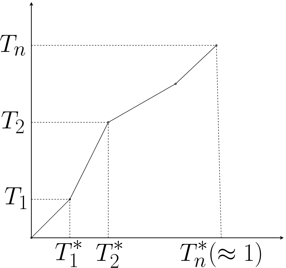
Figure 2: Plot of $A_{t}$ vs $t$ for a fixed $\omega$ in the sample space.

Now applying [29, Theorem 17.24, p. 344] we get that $\mathbf{N}$ is a continuous local martingale with respect to the filtration $\mathcal{H}_{t}$ with quadratic variation

$$[\mathbf{N}]=[\mathbf{B}]\circ\mathbf{A}=\mathbf{A},$$ (106)

since $[B]_{t}=t$ [29, Theorem 18.3, p. 352]. Now we follow the proof of [17, Theorem 4.2, p. 170]. Define $\mathbf{W}$ as

$$W_{t}=\int_{0}^{t}\frac{1}{{\psi_{s}}}\,dN_{s}.$$

Then $\mathbf{W}$ is a continuous local martingale with quadratic variation ([29, Lemma 17.10, p.335], noting that $1/\psi_{s}$ is a step process)

$$[W]_{t}=\int_{0}^{t}\frac{1}{{\psi^{2}_{s}}}\,d[N]_{s}=\int_{0}^{t}\frac{1}{{\psi^{2}_{s}}}\psi^{2}_{s}\,ds=t,$$

where we have used [29, Proposition 17.14, p. 338] for the middle equality. Hence $\mathbf{W}$ is a standard Brownian motion with respect to the filtration $\mathcal{H}_{t}$ [29, Theorem 18.3, p. 352].

Noting that there exists a (random) partition $0=t_{0}<t_{1},\dots,<t_{l}=t$ such that $\boldsymbol{\psi}$ is constant on $(t_{k},t_{k+1}]$ for $0\leq k\leq l-1$, we can write

$$\int_{0}^{t}\psi_{s}\,dW_{s}=\sum_{k=0}^{l-1}\psi_{t_{k}}(W_{t_{k+1}}-W_{t_{k}})=\sum_{k=0}^{l-1}\psi_{t_{k}}\frac{1}{\psi_{t_{k}}}(N_{t_{k+1}}-N_{t_{k}})=N_{t}.$$

Thus

$$\int_{0}^{T_{n}^{\ast}}\psi_{s}\,dW_{s}=N_{T_{n}^{\ast}}=B_{A_{T_{n}^{\ast}}}=B_{T_{n}}=S_{n}.$$ (107)

Since $T_{k}^{*}$ is an $\mathcal{H}_{t}$ stopping time for each $k$, $\psi$ is adapted to $\mathcal{H}_{t}$. Since is it left continuous, it is also predictable.

Now we bound $\mathbb{E}[(T_{n}^{\ast}-1)^{2}]$:

$$\mathbb{E}[(T_{n}^{\ast}-1)^{2}] =\mathbb{E}\left[\left(\sum_{j=1}^{n}\frac{\tau_{j}}{n\mathbb{E}[\tau_{j}|\tilde{\mathcal{G}}_{j-1}]}-1\right)^{2}\right]$$

$$=\mathbb{E}\left[\left(\sum_{j=1}^{n}\frac{\tau_{j}-\mathbb{E}[\tau_{j}|\tilde{\mathcal{G}}_{j-1}]}{n\mathbb{E}[\tau_{j}|\tilde{\mathcal{G}}_{j-1}]}\right)^{2}\right]$$

$$\overset{(a)}{\leq}\frac{1}{\nu_{\text{min}}^{2}}\mathbb{E}\left[\left(\sum_{j=1}^{n}{\tau_{j}-\mathbb{E}[\tau_{j}|\tilde{\mathcal{G}}_{j-1}]}\right)^{2}\right]$$

$$\overset{(b)}{=}\frac{1}{\nu_{\text{min}}^{2}}\mathbb{E}\left[\sum_{j=1}^{n}\left({\tau_{j}-\mathbb{E}[\tau_{j}|\tilde{\mathcal{G}}_{j-1}]}\right)^{2}\right]$$

$$\overset{(c)}{\leq}\frac{1}{\nu_{\text{min}}^{2}}\mathbb{E}\left[\sum_{j=1}^{n}\mathbb{E}[\tau^{2}_{j}|\tilde{\mathcal{G}}_{j-1}]\right]$$

$$\overset{(d)}{\leq}\frac{4}{\nu_{\text{min}}^{2}}\mathbb{E}\left[\sum_{j=1}^{n}\mathbb{E}[Z^{4}_{j}|\mathcal{G}_{j-1}]\right]$$

$$\overset{(e)}{\leq}\frac{4}{\nu_{\text{min}}^{2}}\mathbb{E}\left[\sum_{j=1}^{n}\frac{16\mathfrak{i}_{max}^{4}}{n^{2}}\right]$$

$$=\frac{64\mathfrak{i}_{\text{max}}^{4}}{n\nu_{\text{min}}^{2}}$$

$$\overset{(f)}{=}\frac{K_{W}^{(1)}}{n}.$$

Here, (a) follows from (101) and (103),
(b) follows from noting that the sequence $(\tau_{j}-\mathbb{E}[\tau_{j}|\tilde{\mathcal{G}}_{j-1}],1\leq j\leq n)$ is a martingale difference sequence with respect to the filtration $(\tilde{\mathcal{G}}_{j},1\leq j\leq n)$, making $(\sum_{j=1}^{k}\tau_{j}-\mathbb{E}[\tau_{j}|\tilde{\mathcal{G}}_{j-1}],1\leq k\leq n)$ a martingale and the orthogonal increment property of martingales [37, Theorem 5.4.6],
(c) follows from $\mathbb{E}[({\tau_{j}-\mathbb{E}[\tau_{j}|\tilde{\mathcal{G}}_{j-1}]})^{2}|\mathcal{G}_{j-1}]=\mathbb{E}[\tau^{2}_{j}|\tilde{\mathcal{G}}_{j-1}]-\left(\mathbb{E}[\tau_{j}|\tilde{\mathcal{G}}_{j-1}]\right)^{2}$,
(d) follows from (104),
(e) follows since $|Z_{j}|\leq\frac{2}{\sqrt{n}}\mathfrak{i}_{\text{max}}$ a.s. from (98),
(f) follows from defining $K_{W}^{(1)}\mathrel{\mathop{:}}={64\mathfrak{i}_{\text{max}}^{4}}/{\nu_{\text{min}}^{2}}$. ∎

Now define

$${\xi}_{t}\mathrel{\mathop{:}}=-(r_{n}-\kappa)+\int_{0}^{t}{\psi}_{s}\,d{W}_{s}.$$ (108)

We have the following lemma.

Lemma 8.

$$P\left(\int_{0}^{T_{n}^{\ast}}\psi_{s}\,dW_{s}\geq r_{n}\right)\leq P\left(\xi_{1}\geq 0\right)+\delta_{n}.$$

Proof:

$$P\left(\int_{0}^{T_{n}^{\ast}}\psi_{s}\,dW_{s}\geq r_{n}\right)=P\left(\int_{0}^{1}\psi_{s}\,dW_{s}+\theta_{n}\geq r_{n}\right),$$

where we have defined $\theta_{n}$ as

$$\theta_{n}\mathrel{\mathop{:}}=\int_{0}^{\infty}\mathbf{1}\{1<s\leq T_{n}^{\ast}\}\psi_{s}\,dW_{s}-\int_{0}^{\infty}\mathbf{1}\{T_{n}^{\ast}\leq s<1\}\psi_{s}\,dW_{s}.$$

The second moment of $\theta_{n}$ can be bounded as

$$\mathbb{E}[\theta_{n}^{2}] \overset{(a)}{\leq}2\mathbb{E}\left[\left(\int_{0}^{\infty}\mathbf{1}\{1<s\leq T_{n}^{\ast}\}\psi_{s}\,dW_{s}\right)^{2}\right]+2\mathbb{E}\left[\left(\int_{0}^{\infty}\mathbf{1}\{T_{n}^{\ast}\leq s<1\}\psi_{s}\,dW_{s}\right)^{2}\right]$$

$$\overset{(b)}{=}2\mathbb{E}\left[\int_{0}^{\infty}\mathbf{1}\{1<s\leq T_{n}^{\ast}\}\psi^{2}_{s}\,ds\right]+2\mathbb{E}\left[\int_{0}^{\infty}\mathbf{1}\{T_{n}^{\ast}\leq s<1\}\psi^{2}_{s}\,ds\right]$$

$$=2\mathbb{E}\left[\mathbf{1}\{1<T_{n}^{\ast}\}\int_{1}^{T_{n}^{\ast}}\psi^{2}_{s}\,ds\right]+2\mathbb{E}\left[\mathbf{1}\{T_{n}^{\ast}<1\}\int^{1}_{T_{n}^{\ast}}\psi^{2}_{s}\,ds\right]$$

$$\leq 2\nu_{\text{max}}\mathbb{E}[|T_{n}^{\ast}-1|]$$

$$\leq 2\nu_{\text{max}}\sqrt{\mathbb{E}[(T_{n}^{\ast}-1)^{2}]}$$

$$\overset{(c)}{\leq}\frac{K_{W}}{\sqrt{n}}.$$

Here, for (a) we have used the inequality $(a-b)^{2}\leq 2a^{2}+2b^{2}$,
for (b) we have used [17, Problem 2.18, p. 144],
for (c) we have used Lemma 7, and recalling $K_{W}=16\mathfrak{i}_{\text{max}}^{2}\nu_{\text{max}}/\nu_{\text{min}}=2\nu_{\text{max}}\sqrt{K_{W}^{(1)}}$.

Thus

$$P\left(\int_{0}^{T_{n}^{\ast}}\psi_{s}\,dW_{s}\geq r_{n}\right) =P\left(\int_{0}^{1}\psi_{s}\,dW_{s}+\theta_{n}\geq r_{n}\right)$$

$$=P\left(\int_{0}^{1}\psi_{s}\,dW_{s}+\theta_{n}\geq r_{n}\bigcap|\theta_{n}|\leq\kappa\right)+P\left(\int_{0}^{1}\psi_{s}\,dW_{s}+\theta_{n}\geq r_{n}\bigcap|\theta_{n}|>\kappa\right)$$

$$\leq P\left(\int_{0}^{1}\psi_{s}\,dW_{s}\geq r_{n}-\kappa\bigcap|\theta_{n}|\leq\kappa\right)+P\left(\int_{0}^{1}\psi_{s}\,dW_{s}+\theta_{n}\geq r_{n}\bigcap|\theta_{n}|>\kappa\right)$$

$$\leq P\left(\int_{0}^{1}\psi_{s}\,dW_{s}\geq r_{n}-\kappa\right)+P\left(|\theta_{n}|>\kappa\right)$$

$$\leq P\left(\int_{0}^{1}\psi_{s}\,dW_{s}\geq r_{n}-\kappa\right)+\frac{E[\theta_{n}^{2}]}{\kappa^{2}}$$

$$\leq P\left(\int_{0}^{1}\psi_{s}\,dW_{s}\geq r_{n}-\kappa\right)+\frac{K_{W}}{\kappa^{2}\sqrt{n}}$$

$$=P\left(\int_{0}^{1}\psi_{s}\,dW_{s}\geq r_{n}-\kappa\right)+\delta_{n}$$

$$=P\left(\xi_{1}\geq 0\right)+\delta_{n}.\qed$$

Now we apply [38, Corollary 3.7] (see also [39]). There exists a probability space with a measure $\hat{P}$ that supports a process $\hat{\boldsymbol{\xi}}$ and a Brownian motion $\hat{\mathbf{W}}$ such that

$$\hat{\xi}_{t} =-(r_{n}-\kappa)+\int_{0}^{t}\hat{\psi}_{s}(\hat{\xi}_{s})\,d\hat{W}_{s},$$ (109)

$$P\left(\xi_{t}\geq a\right) =\hat{P}\left(\hat{\xi}_{t}\geq a\right),\qquad a\in\mathbb{R},\,t\geq 0,$$ (110)

and $\hat{\psi}_{t}(\cdot)$ satisfies

$$\hat{\psi}^{2}_{t}(u)=\mathbb{E}[\psi^{2}_{t}|{\xi}_{t}=u]\qquad P\text{-}\text{a.s.},\,t\in\mathcal{N}^{c},$$

where $\mathcal{N}$ is a Lebsegue-null set. In particular, we can take $\hat{\psi}_{t}(u)=\sqrt{\mathbb{E}[\psi^{2}_{t}|{\xi}_{t}=u]}$ [40, Section 5.3].

Note that $\boldsymbol{\xi}$ in (108) is an Itô process, where, in general the drift coefficient $\boldsymbol{\psi}$ itself can be a stochastic process. The process $\boldsymbol{\hat{\xi}}$, on the other hand, has deterministic function $\boldsymbol{\hat{\psi}}(\cdot)$ as the drift coefficient and the same one-dimensional law as that of $\boldsymbol{\xi}$ for each $t$.

Since $\hat{\psi}_{t}\in[\sqrt{\nu_{\text{min}}},\sqrt{\nu_{\text{max}}}]$, (108) has a unique solution in distribution [40, Exercise 7.3.3] (see also the discussion after [38, Corollary 3.13]). Thus the setup in (109) is admissible as defined by McNamara in [11]. McNamara [11, Remark 8] shows that if the goal is to maximize $\hat{P}\left(\bar{\xi}_{1}\geq 0\right)$ where

$$\bar{\xi}_{t}=-(r_{n}-\kappa)+\int_{0}^{t}\bar{\psi}_{s}(\bar{\xi}_{s})\,d\hat{W}_{s},$$

by choosing the optimal diffusion coefficient $\bar{\psi}_{s}(\cdot)$, then such optimal diffusion control is given by

$$\bar{\psi}^{\text{opt}}(u)\mathrel{\mathop{:}}=\sqrt{\nu_{\text{min}}}\mathbf{1}\{u>0\}+\sqrt{\nu_{\text{max}}}\mathbf{1}\{u\leq 0\}.$$ (111)

Let the corresponding SDE be

$$\bar{\xi}_{t}^{\text{opt}}\mathrel{\mathop{:}}=-(r_{n}-\kappa)+\int_{0}^{t}\bar{\psi}^{\text{opt}}(\bar{\xi}_{s}^{\text{opt}})\,d\hat{W}_{s}.$$ (112)

Thus

$$\hat{P}\left(\hat{\xi}_{1}\geq 0\right)\leq\hat{P}\left(\bar{\xi}_{1}^{\text{opt}}\geq 0\right).$$ (113)

Using the distribution function of the solution to (111) and (112) (see (52)), we get

$$\hat{P}\left(\bar{\xi}_{1}^{\text{opt}}\geq 0\right)=1-\frac{2\lambda}{1+\lambda}\Phi\left(\frac{r_{n}-\kappa}{\sqrt{\nu_{\text{min}}}}\right),$$ (114)

when $r_{n}-\kappa\leq 0$, and

$$\hat{P}\left(\bar{\xi}_{1}^{\text{opt}}\geq 0\right)=\frac{2}{1+\lambda}-\frac{2}{1+\lambda}\Phi\left(\frac{r_{n}-\kappa}{\sqrt{\nu_{\text{max}}}}\right),$$ (115)

when $r_{n}-\kappa>0$. For our choice of $r_{n}$ in (96), we get

$$\hat{P}\left(\bar{\xi}_{1}^{\text{opt}}\geq 0\right)=1-\varepsilon-2\delta_{n}.$$ (116)

Summarizing the chain of inequalities so far, we have

$$P\left(\sum_{k=1}^{n}\mathfrak{i}^{*}(X_{k},Y_{k})\geq\log\rho_{n}\right) \leq P(S_{n}\geq r_{n})$$

$$=P\left(\int_{0}^{T_{n}^{\ast}}\psi_{s}\,dW_{s}\geq r_{n}\right)$$

$$\leq P\left(\xi_{1}\geq 0\right)+\delta_{n}$$

$$=\hat{P}\left(\hat{\xi}_{1}\geq 0\right)+\delta_{n}$$

$$\leq\hat{P}\left(\bar{\xi}^{\text{opt}}_{1}\geq 0\right)+\delta_{n}$$

$$=1-\varepsilon-\delta_{n}.$$

Thus from (94)

$$\log M_{\textnormal{fb}}^{\ast}(n,\varepsilon)\leq nC+\sqrt{n}r_{n}-\log\frac{K_{W}}{\kappa^{2}\sqrt{n}},$$ (117)

and hence

$$\frac{\log M_{\textnormal{fb}}^{\ast}(n,\varepsilon)-nC}{\sqrt{n}}\leq r_{n}-\frac{1}{\sqrt{n}}\log\frac{K_{W}}{\kappa^{2}\sqrt{n}}.$$

From the definition of $r_{n}$ in (96), and taking $n\to\infty$,

$$\limsup_{n\to\infty}\frac{\log M^{\ast}_{\textnormal{fb}}(n,\varepsilon)-nC}{\sqrt{n}}\leq\begin{cases}\sqrt{\nu_{\text{min}}}\Phi^{-1}\left(\frac{1}{2\lambda}\varepsilon(1+\lambda)\right)+\kappa,&\varepsilon\in(0,\frac{\lambda}{1+\lambda}],\\ \sqrt{\nu_{\text{max}}}\Phi^{-1}\left(\frac{1}{2}[\varepsilon(1+\lambda)+(1-\lambda)]\right)+\kappa,&\varepsilon\in(\frac{\lambda}{1+\lambda},1).\end{cases}$$

Since $\kappa$ is arbitrary, we may take $\kappa\to 0$ to prove the theorem. ∎

VII Very Noisy Channels

We first derive the scaling behavior of various channel parameters ($C_{\zeta}$, $V_{\min,\zeta}$, etc.) with respect to $\zeta$. Recall that the VNC is given by

$$W_{\zeta}(y|x)=\Gamma(y)\left(1+\zeta\lambda(x,y)\right),$$

where $\Gamma$ is a probability distribution on the output alphabet $\mathcal{Y}$, which we may assume, without loss of generality, has full support, $\lambda(x,y)$ satisfies

$$\sum_{y\in\mathcal{Y}}\Gamma(y)\lambda(x,y)=0$$ (118)

for all $x\in\mathcal{X}$, and $\zeta$ is infinitesimally small. Let

$$\lambda_{\text{max}}\mathrel{\mathop{:}}=\max_{x\in\mathcal{X},y\in\mathcal{Y}}|\lambda(x,y)|.$$

We will denote by $K(\Lambda)$ any non-negative constant which depends only on $(\lambda_{\text{max}},|\mathcal{X}|,|\mathcal{Y}|)$. The quantity represented by $K(\Lambda)$ will in general change from line to line in the derivation.

We will use the following approximation throughout the proof:

Lemma 9.

For all $u$ sufficiently close to zero,

$$|\log(1+u)-u|\leq u^{2},$$

$$\left|\log(1+u)-\left(u-\frac{u^{2}}{2}\right)\right|\leq u^{3}.$$

The following lemma gives the scaling of the capacity $C_{\zeta}$ of the above channel.

Lemma 10.

Let $C_{\zeta}$ denote the capacity of $W_{\zeta}$. Then, for all sufficiently small $\zeta$,

$$\left|C_{\zeta}-\zeta^{2}\mathbf{C}\right|\leq\zeta^{3}K(\Lambda).$$

where

$$\mathbf{C}\mathrel{\mathop{:}}=\max_{P\in\mathcal{P}(\mathcal{X})}\frac{1}{2}\sum_{y\in\mathcal{Y}}\Gamma(y)\Bigg{(}\left.\sum_{x\in\mathcal{X}}P(x)\lambda^{2}(x,y)-\left(\sum_{x\in\mathcal{X}}P(x)\lambda(x,y)\right)^{2}\right).$$ (119)

Proof:

Let $\lambda_{P}(y)=\sum_{x\in\mathcal{X}}P(x)\lambda(x,y)$. The channel capacity at $\zeta$ is given by

$$C_{\zeta} =\max_{P\in\mathcal{P}(\mathcal{X})}I(P;W_{\zeta})$$

$$=\max_{P\in\mathcal{P}(\mathcal{X})}\sum_{x\in\mathcal{X},y\in\mathcal{Y}}P(x)\Gamma(y)\left(1+\zeta\lambda(x,y)\right)\log\frac{1+\zeta\lambda(x,y)}{1+\zeta\lambda_{P}(y)}$$

$$\leq\max_{P\in\mathcal{P}(\mathcal{X})}\sum_{x\in\mathcal{X},y\in\mathcal{Y}}P(x)\Gamma(y)\left(1+\zeta\lambda(x,y)\right)\left(\zeta\lambda(x,y)-\frac{\zeta^{2}\lambda^{2}(x,y)}{2}-\zeta\lambda_{P}(y)+\frac{\zeta^{2}\lambda_{P}^{2}(y)}{2}\right)+\zeta^{3}K(\Lambda)$$

$$\overset{(a)}{\leq}\max_{P\in\mathcal{P}(\mathcal{X})}\sum_{y\in\mathcal{Y}}\Gamma(y)\left(\frac{\zeta^{2}}{2}\sum_{x\in\mathcal{X}}P(x)\lambda^{2}(x,y)-\frac{\zeta^{2}}{2}\lambda^{2}_{P}(y)\right)+\zeta^{3}K(\Lambda)$$

$$=\zeta^{2}\mathbf{C}+\zeta^{3}K(\Lambda).$$

Here for (a), we note that $\sum_{y\in\mathcal{Y}}\Gamma(y)\lambda(x,y)=0$, hence all the terms involving $\zeta$ disappear. The terms involving $\zeta^{3}$ have been absorbed in $\zeta^{3}K(\Lambda)$. Similarly, we can show $C_{\zeta}\geq\zeta^{2}\mathbf{C}-\zeta^{3}K(\Lambda)$. ∎

Let $q_{\zeta}^{\ast}$ denote the output distribution corresponding to a capacity-achieving input distribution $P_{\zeta}^{*}$, i.e.,

$$q_{\zeta}^{\ast}(y)=\Gamma(y)(1+\zeta\lambda^{*}_{\zeta}(y)),$$

where

$$\lambda^{*}_{\zeta}(y)\mathrel{\mathop{:}}=\sum_{x\in\mathcal{X}}P_{\zeta}^{*}(x)\lambda(x,y).$$

Here, we note that $|\lambda^{*}_{\zeta}(y)|\leq\lambda_{\text{max}}$, and

$$\sum_{y\in\mathcal{Y}}\Gamma(y)\lambda^{*}_{\zeta}(y)=0.$$ (120)

Also, since $q_{\zeta}^{\ast}$ is unique, $\lambda^{*}_{\zeta}$ is also unique. Define

$$\mathcal{X}_{\zeta}^{*}\mathrel{\mathop{:}}=\left\{x:\mathbb{E}[i^{*}(X,Y)|X=x]=C_{\zeta}\right\}.$$

For $x\notin\mathcal{X}_{\zeta}^{*}$, let

$$\rho_{\zeta,x}\mathrel{\mathop{:}}=C_{\zeta}-\mathbb{E}[i^{*}(X,Y)|X=x],$$

where we note that $\rho_{\zeta,x}>0$ [18, Theorem 4.5.1].

Define, for each $x\in\mathcal{X}$,

$$\nu_{x,\zeta}\mathrel{\mathop{:}}=\text{Var}\left[i^{*}(X,Y)|X=x\right].$$

Lemma 11.

For all sufficiently small $\zeta$, the conditional expectation and variance of $i^{*}(X,Y)$ satisfy, for each $x$,

$$\left|\mathbb{E}[i^{*}(X,Y)|X=x]-\zeta^{2}\Psi_{\zeta,x}\right|\leq\zeta^{3}K(\Lambda),$$

$$\left|\nu_{x,\zeta}-2\zeta^{2}\Psi_{\zeta,x}\right|\leq\zeta^{3}K(\Lambda),$$

where

$$\Psi_{\zeta,x}\mathrel{\mathop{:}}=\frac{1}{2}\sum_{y\in\mathcal{Y}}\Gamma(y)\left(\lambda(x,y)-\lambda^{*}_{\zeta}(y)\right)^{2}.$$

Hence for $x\in\mathcal{X}_{\zeta}^{*}$,

$$\left|\nu_{x,\zeta}-2C_{\zeta}\right|\leq\zeta^{3}K(\Lambda),$$

and for $x\notin\mathcal{X}_{\zeta}^{*}$,

$$\left|\nu_{x,\zeta}-2(C_{\zeta}-\rho_{\zeta,x})\right|\leq\zeta^{3}K(\Lambda).$$

Proof:

We first note that since $|\lambda^{*}_{\zeta}(y)|\leq\lambda_{\text{max}}$, we have $\Psi_{\zeta,x}\leq K(\Lambda)$. Now consider,

$$\mathbb{E}[i^{*}(X,Y)|X=x] =\sum_{y\in\mathcal{Y}}W_{\zeta}(y|x)\log\frac{W_{\zeta}(y|x)}{q^{\ast}_{\zeta}(y)}$$

$$=\sum_{y\in\mathcal{Y}}\Gamma(y)\left(1+\zeta\lambda(x,y)\right)\log\frac{1+\zeta\lambda(x,y)}{1+\zeta\lambda^{*}_{\zeta}(y)}$$

$$\leq\sum_{y\in\mathcal{Y}}\Gamma(y)\left(1+\zeta\lambda(x,y)\right)\left(\zeta\lambda(x,y)-\frac{\zeta^{2}\lambda^{2}(x,y)}{2}-\zeta\lambda^{*}_{\zeta}(y)+\frac{\zeta^{2}\lambda^{*2}_{\zeta}(y)}{2}\right)+\zeta^{3}K(\Lambda)$$

$$\overset{(a)}{\leq}\sum_{y\in\mathcal{Y}}\Gamma(y)\left(-\frac{\zeta^{2}\lambda^{2}(x,y)}{2}+\frac{\zeta^{2}\lambda^{*2}_{\zeta}(y)}{2}+\zeta^{2}\lambda^{2}(x,y)-\zeta^{2}\lambda(x,y)\lambda^{*}_{\zeta}(y)\right)+\zeta^{3}K(\Lambda)$$

$$=\frac{\zeta^{2}}{2}\sum_{y\in\mathcal{Y}}\Gamma(y)\left(\lambda(x,y)-\lambda^{*}_{\zeta}(y)\right)^{2}+\zeta^{3}K(\Lambda)$$

$$=\zeta^{2}\Psi_{\zeta,x}+\zeta^{3}K(\Lambda).$$

Here, (a) follows from (118), (120), and combining all terms involving $\zeta^{3}$ with $\zeta^{3}K(\Lambda)$.

Similarly, one can show that

$$\mathbb{E}[i^{*}(X,Y)|X=x]\geq\zeta^{2}\Psi_{\zeta,x}-\zeta^{3}K(\Lambda).$$

Using Taylor’s theorem one can show for all sufficiently small $\zeta$,

$$\left|\left(\log\frac{1+\zeta\lambda(x,y)}{1+\zeta\lambda^{*}_{\zeta}(y)}\right)^{2}-\zeta^{2}(\lambda(x,y)-\lambda^{*}_{\zeta}(y))^{2}\right|\leq\zeta^{3}K(\Lambda).$$

Thus,

$$\mathbb{E}\left[(i^{*}(X,Y))^{2}|X=x\right] =\sum_{y\in\mathcal{Y}}\Gamma(y)\left(1+\zeta\lambda(x,y)\right)\left(\log\frac{1+\zeta\lambda(x,y)}{1+\zeta\lambda^{*}_{\zeta}(y)}\right)^{2}$$

$$\leq\sum_{y\in\mathcal{Y}}\Gamma(y)\left(1+\zeta\lambda(x,y)\right)\left(\zeta^{2}(\lambda(x,y)-\lambda^{*}_{\zeta}(y))^{2}\right)+\zeta^{3}K(\Lambda)$$

$$\leq\zeta^{2}\sum_{y\in\mathcal{Y}}\Gamma(y)(\lambda(x,y)-\lambda^{*}_{\zeta}(y))^{2}+\zeta^{3}K(\Lambda)$$

$$=2\zeta^{2}\Psi_{\zeta,x}+\zeta^{3}K(\Lambda).$$

Hence,

$$\nu_{x,\zeta} =\text{Var}\left[i^{*}(X,Y)|X=x\right]$$

$$=\mathbb{E}\left[(i^{*}(X,Y))^{2}|X=x\right]-(\mathbb{E}[i^{*}(X,Y)|X=x])^{2}$$

$$\leq 2\zeta^{2}\Psi_{\zeta,x}+\zeta^{3}K(\Lambda).$$

Note that $\mathbb{E}[i^{*}(X,Y)|X=x]^{2}\leq\zeta^{4}K(\Lambda)$. This gives,

$$\nu_{x,\zeta} \geq 2\zeta^{2}\Psi_{\zeta,x}-\zeta^{3}K(\Lambda).$$

Since for $x\in\mathcal{X}_{\zeta}^{*}$, $\mathbb{E}\left[i^{*}(X,Y)|X=x\right]=C_{\zeta}$, for $x\in\mathcal{X}_{\zeta}^{*}$ we get

$$\left|\nu_{x,\zeta}-2C_{\zeta}\right|\leq\zeta^{3}K(\Lambda),$$

and for $x\notin\mathcal{X}_{\zeta}^{*}$,

$$\left|\nu_{x,\zeta}-2(C_{\zeta}-\rho_{\zeta,x})\right|\leq\zeta^{3}K(\Lambda).$$

∎

Recall that $V_{\text{min},\zeta}$ and $V_{\text{max},\zeta}$ are defined as

$$V_{\text{min},\zeta}\mathrel{\mathop{:}}=\min_{P\in\Pi_{W_{\zeta}}^{*}}\sum_{x\in\mathcal{X}}P(x)\nu_{x,\zeta},$$

$$V_{\text{max},\zeta}\mathrel{\mathop{:}}=\max_{P\in\Pi_{W_{\zeta}}^{*}}\sum_{x\in\mathcal{X}}P(x)\nu_{x,\zeta},$$

where $\Pi_{W_{\zeta}}^{*}$ is the set of capacity-achieving probability distributions.

Lemma 12.

For all sufficiently small $\zeta$, $V_{\text{min},\zeta}$ and $V_{\text{max},\zeta}$ satisfy

$$\left|V_{\text{min},\zeta}-2C_{\zeta}\right|\leq\zeta^{3}K(\Lambda),$$

$$\left|V_{\text{min},\zeta}-2\zeta^{2}\mathbf{C}\right|\leq\zeta^{3}K(\Lambda)$$

$$\left|V_{\text{max},\zeta}-2C_{\zeta}\right|\leq\zeta^{3}K(\Lambda),$$

$$\left|V_{\text{max},\zeta}-2\zeta^{2}\mathbf{C}\right|\leq\zeta^{3}K(\Lambda).$$

Proof:

Note that if $P\in\Pi_{W_{\zeta}}^{*}$, then the support of $P$ is contained in $\mathcal{X}_{\zeta}^{*}$. Thus from Lemma 11 we get $\left|V_{\text{min},\zeta}-2C_{\zeta}\right|\leq\zeta^{3}K(\Lambda)$. Moreover since from Lemma 10, $|C_{\zeta}-\zeta^{2}\mathbf{C}|\leq\zeta^{3}K(\Lambda)$, the inequality $\left|V_{\text{min},\zeta}-2\zeta^{2}\mathbf{C}\right|\leq\zeta^{3}K(\Lambda)$ follows. The second set of inequalities for $V_{\text{max},\zeta}$ can be deduced similarly. ∎

From Lemma 12, we can conclude that $V_{\text{max},\zeta}\approx V_{\text{min},\zeta}$. Thus taking a hint from Theorem 3, we expect that feedback will not improve the performance of VNCs with respect to the second order coding rate. However, since we have not shown that $V_{\text{max},\zeta}=V_{\text{min},\zeta}$, Theorem 3 cannot be directly applied here. Since $\nu_{x,\zeta}$ is not constant over $x$, even asymptotically, Theorem 4 cannot be applied either. Thus we prove the converse with a different strategy.

Since $\nu_{x,\zeta}\approx 2C_{\zeta}$ for $x\in\mathcal{X}_{\zeta}^{*}$, and for $x\notin\mathcal{X}_{\zeta}^{*}$, we have that $\nu_{x,\zeta}\lesssim 2C_{\zeta}$, to obtain the converse we will add non-negative random variables whenever the input $X_{k}\notin\mathcal{X}_{\zeta}^{*}$ to “equalize” the conditional variance. The following lemma shows the existence of such random variables with desirable properties so that we can apply martingale convergence results. This will yield a proper upper on bound on the maximum possible message set size for sufficiently small $\zeta$.

Lemma 13.

We can extend the given probability space to define a sequence of non-negative random variables $\{\xi_{k}\}_{k=1}^{n}$, such that with $Z_{k}=i^{*}(X_{k},Y_{k})+\xi_{k}-C_{\zeta}$, $\mathcal{F}_{k}=\sigma(Z_{1},\dots,Z_{k})$, and for all sufficiently small $\zeta$,

$$|Z_{k}|\leq 3\,\quad\mbox{a.s.},$$

$$\mathbb{E}[Z_{k}|\mathcal{F}_{k-1}]=0\quad\mbox{a.s.},$$

$$V_{\text{min},\zeta}-\zeta^{3}K(\Lambda)\leq\mathbb{E}[Z^{2}_{k}]\leq V_{\text{min},\zeta}+\zeta^{3}K(\Lambda),$$

$$V_{\text{max},\zeta}-\zeta^{3}K(\Lambda)\leq\mathbb{E}[Z^{2}_{k}]\leq V_{\text{max},\zeta}+\zeta^{3}K(\Lambda),$$

$$\left\|\frac{\sum_{k=1}^{n}\mathbb{E}[Z^{2}_{k}|\mathcal{F}_{k-1}]}{\sum_{k=1}^{n}\mathbb{E}[Z^{2}_{k}]}-1\right\|_{\infty}^{1/2}\leq\sqrt{\zeta}K(\Lambda).$$

Proof:

For each $x\notin\mathcal{X}_{\zeta}^{*}$, define $\{\xi_{x,k}\}_{k=1}^{n}$ to be a sequence of i.i.d. random variables, independent of all other random variables such that

$$P(\xi_{x,k}=\rho_{\zeta,x}+2)=1-P(\xi_{x,k}=0)=\frac{\rho_{\zeta,x}}{\rho_{\zeta,x}+2}.$$

The variance of the above random variable is

$$\text{Var}[\xi_{x,k}] =\mathbb{E}[(\xi_{x,k})^{2}]-\left(\mathbb{E}[\xi_{x,k}]\right)^{2}$$

$$=\frac{\rho_{\zeta,x}}{(\rho_{\zeta,x}+2)}(\rho_{\zeta,x}+2)^{2}-\left(\frac{\rho_{\zeta,x}}{(\rho_{\zeta,x}+2)}(\rho_{\zeta,x}+2)\right)^{2}$$

$$=2\rho_{\zeta,x}.$$

Let

$$\xi_{k}=\sum_{x\notin\mathcal{X}_{\zeta}^{*}}\xi_{x,k}\mathbf{1}\{X_{k}=x\}.$$

Then,

$$|Z_{k}| \leq|i^{*}(X_{k},Y_{k})|+\xi_{k}+C_{\zeta}$$

$$\leq|i^{*}(X_{k},Y_{k})|+\max_{x\notin\mathcal{X}_{\zeta}^{*}}\rho_{\zeta,x}+2+C_{\zeta}$$

$$\leq 3\quad\mbox{a.s.},$$

for all sufficiently small $\zeta$. Let $\mathcal{G}_{k}=\sigma(M,Y_{1},\xi_{1},\dots,Y_{k},\xi_{k})$. We note that $X_{k}$ is $\mathcal{G}_{k-1}$ measurable (since the message $M$ and past outputs $(Y_{1},\dots,Y_{k-1})$ determine the input $X_{k}$) and $\mathcal{F}_{k}\subseteq\mathcal{G}_{k}$. Thus,

$$\mathbb{E}[i^{*}(X_{k},Y_{k})|\mathcal{G}_{k-1}] =\mathbb{E}[i^{*}(X_{k},Y_{k})|X_{k}]$$

$$=C_{\zeta}-\rho_{\zeta,X_{k}}\mathbf{1}\{X_{k}\notin\mathcal{X}_{\zeta}^{*}\}.$$

Then,

$$\mathbb{E}[Z_{k}|\mathcal{G}_{k-1}] =C_{\zeta}-\rho_{\zeta,X_{k}}\mathbf{1}\{X_{k}\notin\mathcal{X}_{\zeta}^{*}\}+\rho_{\zeta,X_{k}}\mathbf{1}\{X_{k}\notin\mathcal{X}_{\zeta}^{*}\}-C_{\zeta}$$

$$=0.$$

Taking the conditional expectation with respect to $\mathcal{F}_{k-1}$, and since $\mathcal{F}_{k-1}\subseteq\mathcal{G}_{k-1}$,

$$\mathbb{E}[Z_{k}|\mathcal{F}_{k-1}]=0.$$

Also,

$$\mathbb{E}[Z^{2}_{k}|\mathcal{G}_{k-1}]= \text{Var}[Z_{k}|\mathcal{G}_{k-1}]$$

$$\overset{}{=} \text{Var}[i^{*}(X_{k},Y_{k})+\xi_{k}|\mathcal{G}_{k-1}]$$

$$\overset{(a)}{=} \text{Var}[i^{*}(X_{k},Y_{k})|\mathcal{G}_{k-1}]+\text{Var}[\xi_{k}|\mathcal{G}_{k-1}]$$

$$\overset{(b)}{\leq} \,2C_{\zeta}-2\rho_{\zeta,X_{k}}\mathbf{1}\{X_{k}\notin\mathcal{X}_{\zeta}^{*}\}+\zeta^{3}K(\Lambda)+2\rho_{\zeta,X_{k}}\mathbf{1}\{X_{k}\notin\mathcal{X}_{\zeta}^{*}\}$$

$$= \,2C_{\zeta}+\zeta^{3}K(\Lambda).$$ (121)

Here (a) follows since given $X_{k}$, $i^{*}(X_{k},Y_{k})$ and $\xi_{k}$ are conditionally independent, and
(b) follows from Lemma 11 and noting that $\text{Var}[\xi_{x,k}]=2\rho_{\zeta,x}$.

Similarly

$$\mathbb{E}[Z^{2}_{k}|\mathcal{G}_{k-1}]\geq 2C_{\zeta}-\zeta^{3}K(\Lambda).$$ (122)

Thus from Lemma 12, (121) and (122),

$$V_{\text{min},\zeta}-\zeta^{3}K(\Lambda)\leq\mathbb{E}[Z^{2}_{k}|\mathcal{G}_{k-1}]\leq V_{\text{min},\zeta}+\zeta^{3}K(\Lambda),$$

$$V_{\text{max},\zeta}-\zeta^{3}K(\Lambda)\leq\mathbb{E}[Z^{2}_{k}|\mathcal{G}_{k-1}]\leq V_{\text{max},\zeta}+\zeta^{3}K(\Lambda).$$

Once again taking the conditional expectation with respect to $\mathcal{F}_{k-1}$,

$$V_{\text{min},\zeta}-\zeta^{3}K(\Lambda)\leq\mathbb{E}[Z^{2}_{k}|\mathcal{F}_{k-1}]\leq V_{\text{min},\zeta}+\zeta^{3}K(\Lambda),$$ (123)

$$V_{\text{max},\zeta}-\zeta^{3}K(\Lambda)\leq\mathbb{E}[Z^{2}_{k}|\mathcal{F}_{k-1}]\leq V_{\text{max},\zeta}+\zeta^{3}K(\Lambda).$$

Now consider

$$\frac{\sum_{k=1}^{n}\mathbb{E}[Z^{2}_{k}|\mathcal{F}_{k-1}]}{\sum_{k=1}^{n}\mathbb{E}[Z^{2}_{k}]}-1 \leq\frac{V_{\text{min},\zeta}+\zeta^{3}K(\Lambda)}{V_{\text{min},\zeta}-\zeta^{3}K(\Lambda)}-1$$

$$=\frac{2\zeta^{3}K(\Lambda)}{V_{\text{min},\zeta}-\zeta^{3}K(\Lambda)}.$$

Here, we note that for the last equality to hold, the constants $K(\Lambda)$ appearing in the left and right terms of (123) should be equal. If they are not, we simply replace each by the maximum of the two constants. Similarly,

$$\frac{\sum_{k=1}^{n}\mathbb{E}[Z^{2}_{k}|\mathcal{F}_{k-1}]}{\sum_{k=1}^{n}\mathbb{E}[Z^{2}_{k}]}-1\geq-\frac{2\zeta^{3}K(\Lambda)}{V_{\text{min},\zeta}+\zeta^{3}K(\Lambda)}.$$

Thus,

$$\left\|\frac{\sum_{k=1}^{n}\mathbb{E}[Z^{2}_{k}|\mathcal{F}_{k-1}]}{\sum_{k=1}^{n}\mathbb{E}[Z^{2}_{k}]}-1\right\|_{\infty}^{1/2} \leq\left(\frac{2\zeta^{3}K(\Lambda)}{V_{\text{min},\zeta}-\zeta^{3}K(\Lambda)}\right)^{1/2}$$

$$\leq\sqrt{\zeta}K(\Lambda),$$

where the last inequality is due to Lemma 12. ∎

Now we give the proof of Theorem 5. Define

$$\kappa_{\zeta,n} \mathrel{\mathop{:}}=K(\Lambda)\left(\frac{\log(n)}{\zeta^{3}\sqrt{n}}+\sqrt{\zeta}\right)$$ (124)

$$r_{\zeta,n} \mathrel{\mathop{:}}=\begin{cases}\sqrt{\left(V_{\text{min},\zeta}-\zeta^{3}K(\Lambda)\right)}\Phi^{-1}(\varepsilon+\kappa_{\zeta,n}),&0<\varepsilon\leq\frac{1}{2}-\kappa_{\zeta,n}\\ \sqrt{\left(V_{\text{max},\zeta}+\zeta^{3}K(\Lambda)\right)}\Phi^{-1}(\varepsilon+\kappa_{\zeta,n}),&\frac{1}{2}-\kappa_{\zeta,n}<\varepsilon<1.\end{cases}$$ (125)

$$\rho_{\zeta,n} \mathrel{\mathop{:}}=\exp(nC_{\zeta}+\sqrt{n}r_{n}),$$ (126)

Now defining $\{\xi_{k}\}_{k=1}^{n}$ as a sequence of random variables as in Lemma 13, consider the following chain of inequalities:

$$P\left(\sum_{k=1}^{n}i^{*}(X_{k},Y_{k})\geq\log\rho_{\zeta,n}\right) \overset{(a)}{\leq}P\left(\sum_{k=1}^{n}i^{*}(X_{k},Y_{k})+\xi_{k}\geq\log\rho_{\zeta,n}\right)$$

$$\overset{(b)}{=}P\left(\sum_{k=1}^{n}Z_{k}\geq\sqrt{n}r_{\zeta,n}\right)$$

$$\overset{(c)}{\leq}P\left(\frac{1}{\sqrt{\sum_{k=1}^{n}\mathbb{E}[Z^{2}_{k}]}}\sum_{k=1}^{n}Z_{k}\geq\Phi^{-1}(\varepsilon+2\kappa_{\zeta,n})\right)$$

$$\overset{(d)}{\leq}1-\varepsilon-2\kappa_{\zeta,n}+\chi\cdot\left(\frac{n\log(n)}{\left(\sum_{k=1}^{n}\mathbb{E}[Z^{2}_{k}]\right)^{3/2}}+\left\|\frac{\sum_{k=1}^{n}\mathbb{E}[Z^{2}_{k}|\mathcal{F}_{k-1}]}{\sum_{k=1}^{n}\mathbb{E}[Z^{2}_{k}]}-1\right\|_{\infty}^{1/2}\right)$$

$$\overset{(e)}{\leq}1-\varepsilon-2\kappa_{\zeta,n}+\left(K(\Lambda)\frac{\log(n)}{\zeta^{3}\sqrt{n}}+K(\Lambda)\sqrt{\zeta}\right)$$

$$=1-\varepsilon-\kappa_{\zeta,n}.$$ (127)

Here, (a) follows since $\xi_{k}$ is a non-negative random variable,
(b) follows from setting $Z_{k}$ as in Lemma 13,
(c) follows since $n(V_{\text{min},\zeta}-\zeta^{3}K(\Lambda))\leq\sum_{k=1}^{n}\mathbb{E}[Z^{2}_{k}]\leq n(V_{\text{max},\zeta}+\zeta^{3}K(\Lambda))$ due to Lemma 13,
(d) follows from the martingale central limit theorem [33, Corollary to Theorem 2], and taking the constant as $\chi$ (which does not depend upon the channel or $n$), and
(e) follows from noting that $\left(\sum_{k=1}^{n}\mathbb{E}[Z^{2}_{k}]\right)^{3/2}\geq n\sqrt{n}(2\zeta^{2}\mathbf{C}-\zeta^{3}K(\Lambda))^{3/2}$, and then absorbing $\chi$ into $K(\Lambda)$.

Invoking Lemma 15 from the Appendix with $q_{\zeta}(\mathbf{y}^{n})=\prod_{i=1}^{n}q_{\zeta}^{\ast}(y_{i})$, we get

$$\log M^{\ast}_{\textnormal{fb},\zeta}(n,\varepsilon)\leq\log\rho_{\zeta,n}-\log\kappa_{\zeta,n}\leq nC_{\zeta}+\sqrt{n}r_{\zeta,n}-\log\kappa_{\zeta,n}.$$

If $0<\varepsilon<\frac{1}{2}$,

$$\limsup_{n\to\infty}\frac{\log M^{\ast}_{\textnormal{fb},\zeta}(n,\varepsilon)-nC_{\zeta}}{\sqrt{nV_{\text{min},\zeta}}}\leq\sqrt{1-\frac{\zeta^{3}K(\Lambda)}{V_{\text{min},\zeta}}}\Phi^{-1}(\varepsilon+K(\Lambda)\sqrt{\zeta}),$$

and hence,

$$\limsup_{\zeta\to 0}\limsup_{n\to\infty}\frac{\log M^{\ast}_{\textnormal{fb},\zeta}(n,\varepsilon)-nC_{\zeta}}{\sqrt{nV_{\text{min},\zeta}}}\leq\Phi^{-1}(\varepsilon).$$

Similarly, when $\frac{1}{2}\leq\varepsilon<1$,

$$\limsup_{\zeta\to 0}\limsup_{n\to\infty}\frac{\log M^{\ast}_{\textnormal{fb},\zeta}(n,\varepsilon)-nC_{\zeta}}{\sqrt{nV_{\text{max},\zeta}}}\leq\Phi^{-1}(\varepsilon).$$

Since $V_{\text{min},\zeta}/V_{\text{max},\zeta}\rightarrow 1$ as $\zeta\rightarrow 0$ by Lemma 12, the conclusion follows. ∎

As noted in the introduction, the problem of maximizing the second-order coding rate with feedback is related to the design of controlled random walks.

Definition 13.

A controller is a function $F:(\mathcal{X}\times\mathcal{Y})^{\ast}\rightarrow\mathcal{P}(\mathcal{X})$.

We shall sometimes write $F(\cdot|\mathbf{x}^{k},\mathbf{y}^{k})$ for $F(\mathbf{x}^{k},\mathbf{y}^{k})(\cdot)$. Given a controller $F$, let $F\circ W$ denote the distribution

$$(F\circ W)(\mathbf{x}^{n},\mathbf{y}^{n})=\prod_{k=1}^{n}F(x_{k}|\mathbf{x}^{k-1},\mathbf{y}^{k-1})W(y_{k}|x_{k})$$ (128)

and let $FW(\mathbf{y}^{n})$ denote the marginal over $\mathbf{Y}^{n}$ induced by $F\circ W$.

The following lemma shows that any controller gives rise to an achievable second-order coding rate. The idea is to use the controller to generate a random ensemble of feedback codes and then use a technique that dates back to Shannon [41] to bound the error probability of this ensemble.

Lemma 14 (Achievability).

For any controller $F$ and any $n$, $\theta$, and rate $R$,

$$\bar{\textnormal{P}}_{\textnormal{e},\textnormal{fb}}(n,R)\leq(F\circ W)\left(\frac{1}{n}\log\frac{W(\mathbf{Y}^{n}|\mathbf{X}^{n})}{FW(\mathbf{Y}^{n})}\leq R+\theta\right)+e^{-n\theta}.$$ (129)

Thus, if for some $\alpha$ and $\varepsilon$,

$$\limsup_{n\to\infty}\inf_{F}(F\circ W)\left(\sum_{k=1}^{n}\log\frac{W(Y_{k}|X_{k})}{(FW)(Y_{k}|\mathbf{Y}^{k-1})}\leq nC+\alpha\sqrt{n}\right)<\varepsilon,$$ (130)

then

$$\liminf_{n\to\infty}\frac{\log M^{\ast}_{\textnormal{fb}}(n,\varepsilon)-nC}{\sqrt{n}}\geq\alpha.$$ (131)

Proof:

We begin by showing (129). Consider a random code in which, for each message, the channel input at time $k$ when the past inputs are $\mathbf{x}^{k-1}$ and the past outputs are $\mathbf{y}^{k-1}$ is chosen according to $F(\cdot|\mathbf{x}^{k-1},\mathbf{y}^{k-1})$. That is, $f(m,\mathbf{y}^{k-1})$ is chosen randomly according to

$$F(\cdot|(f(m,\emptyset),f(m,y_{1}),\ldots,f(m,\mathbf{y}^{k-2})),\mathbf{y}^{k-1}).$$ (132)

Given $\mathbf{y}^{n}$, the decoder selects the message with the lowest index that achieves the minimum over $m$ of

$$\prod_{k=1}^{n}W(y_{k}|f(m,\mathbf{y}^{k-1})).$$ (133)

By the union bound and other standard steps, the ensemble average error probability of this code is upper bounded by

$$\sum_{\mathbf{x}^{n},\mathbf{y}^{n}}(F\circ W)(\mathbf{x}^{n},\mathbf{y}^{n}){\mathbf{1}}{\left\{\frac{1}{n}\log\frac{W(\mathbf{y}^{n}|\mathbf{x}^{n})}{FW(\mathbf{y}^{n})}\leq R+\theta\right\}}$$ (134)

$$\phantom{\sum}+e^{nR}\sum_{\mathbf{x}^{n},\mathbf{y}^{n}}(F\circ W)(\mathbf{x}^{n},\mathbf{y}^{n})\sum_{\tilde{\mathbf{x}}^{n}:W(\mathbf{y}^{n}|\tilde{\mathbf{x}}^{n})\geq W(\mathbf{y}^{n}|\mathbf{x}^{n})}\prod_{k=1}^{n}F(\tilde{x}_{k}|\tilde{\mathbf{x}}^{k-1},\mathbf{y}^{k-1}){\mathbf{1}}\left\{\frac{1}{n}\log\frac{W(\mathbf{y}^{n}|\mathbf{x}^{n})}{FW(\mathbf{y}^{n})}>R+\theta\right\}$$ (135)

$$\leq(F\circ W)\left(\frac{1}{n}\log\frac{W(\mathbf{Y}^{n}|\mathbf{X}^{n})}{FW(\mathbf{Y}^{n})}\leq R+\theta\right)$$ (136)

$$\phantom{\sum}+e^{nR}\sum_{\mathbf{y}^{n}}FW(\mathbf{y}^{n})\sum_{\tilde{\mathbf{x}}^{n}}\prod_{k=1}^{n}F(\tilde{x}_{k}|\tilde{\mathbf{x}}^{k-1},\mathbf{y}^{k-1}){\mathbf{1}}\left\{\frac{1}{n}\log\frac{W(\mathbf{y}^{n}|\tilde{\mathbf{x}}^{n})}{FW(\mathbf{y}^{n})}>R+\theta\right\}$$ (137)

$$\leq(F\circ W)\left(\frac{1}{n}\log\frac{W(\mathbf{Y}^{n}|\mathbf{X}^{n})}{FW(\mathbf{Y}^{n})}\leq R+\theta\right)$$ (138)

$$\phantom{\sum}+e^{nR}e^{-n(R+\theta)}\sum_{\tilde{\mathbf{x}}^{n}}\sum_{\mathbf{y}^{n}}\prod_{k=1}^{n}F(\tilde{x}_{k}|\tilde{\mathbf{x}}^{k-1},\mathbf{y}^{k-1})W(y_{k}|\tilde{x}_{k}),$$ (139)

which implies (129). Now suppose (130) holds and in (129), select $R=C+\alpha^{\prime}/\sqrt{n}$ and $\theta=n^{-\beta}$ for some $1/2<\beta<1$ and $\alpha^{\prime}<\alpha$. Then we have

$$\limsup_{n\rightarrow\infty}\bar{\textnormal{P}}_{\textnormal{e},\textnormal{fb}}\left(n,C+\frac{\alpha^{\prime}}{\sqrt{n}}\right)\leq\limsup_{n\rightarrow\infty}\inf_{F}(F\circ W)\left(\frac{1}{n}\log\frac{W(\mathbf{Y}^{n}|\mathbf{X}^{n})}{FW(\mathbf{Y}^{n})}\leq C+\frac{\alpha^{\prime}}{\sqrt{n}}+\frac{1}{n^{\beta}}\right).$$ (140)

Thus if (130) holds we have

$$\limsup_{n\rightarrow\infty}\bar{\textnormal{P}}_{\textnormal{e},\textnormal{fb}}\left(n,C+\frac{\alpha^{\prime}}{\sqrt{n}}\right)<\varepsilon,$$ (141)

since $\alpha^{\prime}<\alpha$. This implies that eventually,

$$\log M^{\ast}_{\textnormal{fb}}(n,\varepsilon)\geq nC+\alpha^{\prime}\sqrt{n}.$$ (142)

Since this holds for any $\alpha^{\prime}<\alpha$, (131) follows. ∎

The next result is used repeatedly in the paper as a starting point in proving converses. A similar inequality to (143) can be found in [12, (42)]. Observe that (144) and (145), which are a consequence of (143), are nearly a converse of (130) and (131) above.

Lemma 15 (Converse).

For any $\rho>0$ and $\varepsilon>0$

$$\log M_{\textnormal{fb}}^{\ast}(n,\varepsilon)\leq\sup_{F}\inf_{q\in\mathcal{P}(\mathcal{Y}^{n})}\left(\log\rho-\log\left[\left(1-\varepsilon-(F\circ W)\left(\sum_{k=1}^{n}\log\frac{W(Y_{k}|X_{k})}{q(Y_{k}|\mathbf{Y}^{k-1})}>\log\rho\right)\right)^{+}\right]\right).$$ (143)

In particular, if for some $\alpha$ and $\varepsilon$,

$$\liminf_{n\to\infty}\inf_{F}\sup_{q\in\mathcal{P}(\mathcal{Y}^{n})}(F\circ W)\left(\sum_{k=1}^{n}\log\frac{W(Y_{k}|X_{k})}{q(Y_{k}|\mathbf{Y}^{k-1})}\leq nC+\alpha\sqrt{n}\right)>\varepsilon,$$ (144)

then

$$\limsup_{n\to\infty}\frac{\log M^{\ast}_{\textnormal{fb}}(n,\varepsilon)-nC}{\sqrt{n}}\leq\alpha.$$ (145)

Proof:

Consider an $(n,R)$ feedback code $(f,g)$ with average error probability at most $\varepsilon$. We will denote this code by $\mathfrak{C}$ and its average error probability by $\varepsilon_{\mathfrak{C}}$. Define

$$M_{\textnormal{fb},\mathfrak{C}}^{\ast}(n)\mathrel{\mathop{:}}=\lceil\exp\left({nR}\right)\rceil.$$

Then

$$M_{\textnormal{fb}}^{\ast}(n,\varepsilon)=\sup_{\mathfrak{C}:\varepsilon_{\mathfrak{C}}\leq\varepsilon}M_{\textnormal{fb},\mathfrak{C}}^{\ast}(n).$$

The code $\mathfrak{C}$ induces a controller $F$ via

$$F(x_{k}|\mathbf{x}^{k-1},\mathbf{y}^{k-1})\mathrel{\mathop{:}}=\frac{1}{M_{\textnormal{fb},\mathfrak{C}}^{\ast}(n)}\sum_{m=1}^{M_{\textnormal{fb},\mathfrak{C}}^{\ast}(n)}\mathbf{1}\{f(m,\mathbf{y}^{k-1})=x_{k}\},$$

which, in fact, does not depend on $\mathbf{x}^{k-1}$. Now consider the problem of hypothesis testing where a random variable $U$ taking values in ${\cal U}$ can have probability measure $P$ or $Q$. Upon observing $U$, the goal is to declare either $U\sim P$ (hypothesis $H_{1}$) or $U\sim Q$ (hypothesis $H_{2}$). Let $\beta_{\alpha}(P,Q)$ denote the minimum attainable error probability under $Q$ when the error probability under $P$ does not exceed $1-\alpha$. Then the Neyman-Pearson lemma [42, Proposition II.D.1, p. 33] guarantees that there exists a (possibly randomized) test $T:{\cal U}\to\{0,1\}$ (where $0$ corresponds to the test selecting $Q$) such that

$$\sum_{u\in{\cal U}}P(u)T(1|u)\geq\alpha,\\ \sum_{u\in{\cal U}}Q(u)T(1|u)=\beta_{\alpha}(P,Q).$$

Then for any $\rho>0$

$$\alpha-\rho\beta_{\alpha}(P,Q) \leq\sum_{u\in{\cal U}}T(1|u)(P(u)-\rho Q(u))$$

$$\leq\sum_{u\in{\cal U}}T(1|u)(P(u)-\rho Q(u))\mathbf{1}\{P(u)>\rho Q(u)\}$$

$$=P\left(\frac{P(u)}{Q(u)}>\rho,T=1\right)-\rho Q\left(\frac{P(u)}{Q(u)}>\rho,T=1\right)$$

$$\leq P\left(\frac{P(u)}{Q(u)}>\rho\right).$$ (146)

Fix a $q\in\mathcal{P}(\mathcal{Y}^{n})$. Applying [20, Theorem 26] (with $Q_{Y|X}=q$, $\varepsilon^{\prime}=1-1/M_{\textnormal{fb},\mathfrak{C}}^{\ast}(n)$; the assertion there is without feedback but one can verify that it applies to the feedback case as well), we get

$$\beta_{1-{\varepsilon_{\mathfrak{C}}}}\left(F\circ W,F\circ q\right)\leq\frac{1}{M_{\textnormal{fb},\mathfrak{C}}^{\ast}(n)}.$$

Moreover, from (146)

$$\alpha\leq(F\circ W)\left(\frac{d(F\circ W)}{d(F\circ q)}>\rho\right)+\rho\beta_{\alpha}\left(F\circ W,F\circ q\right),$$

i.e.,

$$\beta_{1-{\varepsilon_{\mathfrak{C}}}}\left(F\circ W,F\circ q\right)\geq\frac{1}{\rho}\left(1-{\varepsilon_{\mathfrak{C}}}-(F\circ W)\left(\frac{d(F\circ W)}{d(F\circ q)}>\rho\right)\right)^{+}.$$

Thus

$$\log M_{\textnormal{fb},\mathfrak{C}}^{\ast}(n)\leq\log\rho-\log\left[\left(1-{\varepsilon_{\mathfrak{C}}}-(F\circ W)\left(\frac{d(F\circ W)}{d(F\circ q)}>\rho\right)\right)^{+}\right].$$

Using the fact that $\varepsilon_{\mathfrak{C}}\leq\varepsilon$ and that $q$ was arbitrary, we obtain

$$\log M_{\textnormal{fb},\mathfrak{C}}^{\ast}(n)\leq\inf_{q\in\mathcal{P}(\mathcal{Y}^{n})}\log\rho-\log\left[\left(1-{\varepsilon}-(F\circ W)\left(\frac{d(F\circ W)}{d(F\circ q)}>\rho\right)\right)^{+}\right].$$

Taking the supremum over all controllers $F$ and noting that

$$\frac{d(F\circ W)}{d(F\circ q)}=\prod_{k=1}^{n}\frac{W(y_{k}|x_{k})}{q(y_{k}|\mathbf{y}^{k-1})},$$

we get

$$\log M_{\textnormal{fb}}^{\ast}(n)\leq\sup_{F}\inf_{q\in\mathcal{P}(\mathcal{Y}^{n})}\left(\log\rho-\log\left[\left(1-\varepsilon-(F\circ W)\left(\sum_{k=1}^{n}\log\frac{W(Y_{k}|X_{k})}{q(Y_{k}|\mathbf{Y}^{k-1})}>\log\rho\right)\right)^{+}\right]\right).$$

This establishes (143). (145) follows directly from (143) and (144). ∎

References

[1]
C. E. Shannon, “The zero error capacity of a noisy channel,” IRE
Trans. Inf. Theory, vol. 2, pp. S8–S19, Sep. 1956.
[2]
Y.-H. Kim, “Feedback capacity of stationary Gaussian channels,”
IEEE Trans. Inf. Theory, vol. 56, no. 1, pp. 57–85, Jan. 2010.
[3]
A. Tchamkerten and İ. E. Telatar, “Variable length coding over an unknown
channel,” IEEE Trans. Inf. Theory, vol. 52, no. 5, pp. 2126–2145,
May 2006.
[4]
M. V. Burnashev, “Data transmission over a discrete channel with feedback.
random transmission time.” Probl. Pered. Inf., vol. 12, no. 4, pp.
10–30, 1976, in Russian.
[5]
J. Schalkwijk and T. Kailath, “A coding scheme for additive noise channels
with feedback–I: No bandwidth constraint,” IEEE Trans. Inf.
Theory, vol. 12, no. 2, pp. 172–182, Apr. 1966.
[6]
J. Schalkwijk, “A coding scheme for additive noise channels with
feedback–II: Band-limited signals,” IEEE Trans. Inf. Theory,
vol. 12, no. 2, pp. 183–189, Apr. 1966.
[7]
E. R. Berlekamp, “Block coding with noiseless feedback,” Ph.D. dissertation,
MIT, Cambridge, MA, 1964.
[8]
N. T. Gaarder and J. K. Wolf, “The capacity region of a multiple-access
discrete memoryless channel can increase with feedback,” IEEE Trans.
Inf. Theory, vol. 21, no. 1, pp. 100–102, Jan. 1975.
[9]
Y. Polyanskiy, H. V. Poor, and S. Verdú, “Feedback in the non-asymptotic
regime,” IEEE Trans. on Info. Theory, vol. 57, no. 8, pp. 4903–4925,
Aug 2011.
[10]
T. M. Cover and J. A. Thomas, Elements of Information Theory,
2nd ed. Wiley-Interscience, 2006.
[11]
J. M. McNamara, “Optimal control of the diffusion coefficient of a simple
diffusion process,” Mathematics of Operations Research, vol. 8,
no. 3, pp. 373–380, 1983.
[12]
S. L. Fong and V. Y. F. Tan, “A tight upper bound on the second-order coding
rate of the parallel Gaussian channel with feedback,” IEEE Trans. on
Info. Theory, vol. 63, no. 10, pp. 6474–6486, Oct 2017.
[13]
B. Reiffen, “A note on ‘very noisy channels’,” Information and
Control, vol. 6, no. 2, pp. 126 – 130, 1963.
[14]
E. E. Majani, “A model for the study of very noisy channels, and
applications,” Ph.D. dissertation, California Institute of Technology, 1987.
[15]
A. Lapidoth, İ. E. Telatar, and R. Urbanke, “On wide-band broadcast
channels,” IEEE Trans. on Info. Theory, vol. 49, no. 12, pp.
3250–3258, Dec 2003.
[16]
I. Csiszár and J. Körner, Information Theory: Coding Theorems for
Discrete Memoryless Systems. Cambridge University Press, 2011.
[17]
I. Karatzas and S. Shreve, Brownian Motion and Stochastic
Calculus. Springer-Verlag New York
Inc., 1988.
[18]
R. G. Gallager, Information Theory and Reliable Communication. New York, NY, USA: John Wiley & Sons, Inc.,
1968.
[19]
V. Strassen, “Asymptotische Abschatzungen in Shannon’s
Informationstheorie,” in Trans. Third Prague Conf Information
Theory, Prague, 1962, pp. 689–723.
[20]
Y. Polyanskiy, H. V. Poor, and S. Verdú, “Channel coding rate in the
finite blocklength regime,” IEEE Trans. on Info. Theory, vol. 56,
no. 5, pp. 2307–2359, May 2010.
[21]
S. L. Fong and V. Y. F. Tan, private communication, 2017.
[22]
N. V. Shende and A. B. Wagner, “On very noisy channels with feedback,” in
55th Annual Allerton Conference on Communication, Control, and
Computing, Oct 2017, pp. 1–8.
[23]
S. Lee and K. A. Winick, “Very noisy channels, reliability functions, and
exponentially optimum codes,” IEEE Trans. Inf. Theory, vol. 40,
no. 3, pp. 647–661, May 1994.
[24]
V. Y. Korolev and I. G. Shevtsova, “A new moment-type estimate of convergence
rate in the Lyapunov theorem,” Theory of Probability and its
Applications, vol. 55, no. 3, pp. 505–509, 2011.
[25]
A. C. Berry, “The accuracy of the Gaussian approximation to the sum of
independent variates,” Transactions of the American Mathematical
Society, vol. 49, no. 1, pp. 122–136, 1941.
[26]
C.-G. Esseen, “Fourier analysis of distribution functions. A mathematical
study of the Laplace-Gaussian law,” Acta Math., vol. 77, pp.
1–125, 1945.
[27]
B. Øksendal, Stochastic Differential Equations: An Introduction with
Applications, 5th ed. Springer-Verlag
Berlin Heidelberg, 1998.
[28]
H. J. Kushner, “On the weak convergence of interpolated Markov chains to a
diffusion,” The Annals of Probability, vol. 2, no. 1, pp. 40–50, 02
1974.
[29]
O. Kallenberg, Foundations of Modern Probability, 2nd ed. Springer-Verlag, New York, 2002.
[30]
G. L. Kulinich, “On the limit behaviour of the solution of a stochastic
diffusion equation,” Theory of Probability and its Applications,
vol. 12, no. 3, pp. 497–799, Jul. 1967.
[31]
P. Billingsley, Convergence of Probability Measures, 2nd ed. Wiley, 1999.
[32]
G. L. Kulinich, “On necessary and sufficient conditions for convergence of
solutions to one-dimensional stochastic diffusion equations with a nonregular
dependence of the coefficients on a parameter,” Theory of Probability
and its Applications, vol. 27, no. 4, pp. 856–862, 1983.
[33]
E. Bolthausen, “Exact convergence rates in some martingale central limit
theorems,” Ann. Probab., vol. 10, no. 3, pp. 672–688, 1982.
[34]
M. Hayashi, “Information spectrum approch to second-order coding rate in
channel coding,” IEEE Trans. on Info. Theory, vol. 55, no. 11, pp.
4947–4966, Nov 2009.
[35]
B. Bercu, B. Delyon, and E. Rio, Concentration Inequalities for Sums and
Martingales. Springer International
Publishing, 2015.
[36]
O. Barndorff-Nielsen and A. Shiryaev, Change of Time and Change of
Measure. World Scientific Publishing
Co. Pte. Ltd., 2010, vol. 13.
[37]
R. Durrett, Probability: Theory and Examples, 4th ed. Cambridge University Press, 2010.
[38]
G. Brunick and S. Shreve, “Mimicking an Itô process by a solution of
a stochastic differential equation,” The Annals of Applied
Probability, vol. 23, no. 4, pp. 1584–1628, Aug 2013.
[39]
I. Gyöngy, “Mimicking the one-dimensional marginal distributions of
processes having an Ito differential,” Probability Theory and
Related Fields, vol. 71, no. 4, pp. 501–516, Dec 1986.
[40]
D. Stroock and S. Varadhan, Multidimensional Diffusion Processes. Springer Berlin Heidelberg, 2007.
[41]
C. E. Shannon, “Certain results in coding theory for noisy channels,”
Information and Control, vol. 1, no. 1, pp. 6 – 25, 1957.
[42]
H. V. Poor, An Introduction to Signal Detection and Estimation,
2nd ed. Springer-Verlag, 1994.