Reduced dynamics for one and two dark soliton stripes
in the defocusing nonlinear Schrödinger equation: a variational approach

Abstract

We study the dynamics and pairwise interactions of dark soliton stripes in the two-dimensional defocusing nonlinear Schrödinger equation. By employing a variational approach we reduce the dynamics for dark soliton stripes to a set of coupled one-dimensional “filament” equations of motion for the position and velocity of the stripe. The method yields good qualitative agreement with the numerical results as regards the transverse instability of the stripes. We propose a phenomenological amendment that also significantly improves the quantitative agreement of the method with the computations. Subsequently, the method is extended for a pair of symmetric dark soliton stripes that include the mutual interactions between the filaments. The reduced equations of motion are compared with a recently proposed adiabatic invariant method and its corresponding findings and are found to provide a more adequate representation of the original full dynamics for a wide range of cases encompassing perturbations with long and short wavelengths, and combinations thereof.

I Introduction

In the past two decades, the study of coherent structures in the form of dark solitons has been a theme pervading a wide range of areas within Physics. Early examples were more focused on classical physics (including mechanical mech and electrical el lattices), nonlinear optical Kivshar-LutherDavies , as well as magnetic systems mf . More recently, however, there has been a host of additional systems including notably a wide variety of experiments in atomic Bose-Einstein condensates summarized, e.g., in Refs. djf ; SIAMbook , but also realizations in electromagnetic gv , hydrodynamic ww , acoustic chong , plasma plasma and exciton-polariton polar systems among others.

A major thrust within the subject has been offered by the extensive experimental accessibility to such nonlinear waves offered in the context of atomic (but also exciton-polariton) condensates. Here, there has been a variety of techniques of formation of the structures, including wave interference ourmarkus2 ; ourmarkus3 , phase imprinting becker and rapid dragging of laser beams through a trapped BEC engels . Additionally, the structures have offered a variety of intriguing insights in the dynamics through their potential dynamical instabilities (and their avoidance through suitable manipulation of length scales infrared ) which may lead to a variety of vortical (in 2D) and vortex line/ring structures (in 3D), as has also been documented experimentally watching ; jeff ; becker2 ; lamporesi . More recently extensions to multi-component settings have been pursued in the form of dark-bright and dark-dark solitonic states revip and even spinorial realizations of such structures have recently been identified bersano . At the same time, there has been a growing interest in applications including possibilities of atomic matter-wave interferometers in1 and proposals for the use of dark solitons as qubits in BECs qub .

The study of transverse (“snaking”) dynamical instabilities of dark solitons in higher dimensional settings has been a topic of extensive interest since early on kuzne , with much of the early work summarized in the review kidep . Recently, there has been a surge of further interest in the subject aipaper ; aipaper2 ; aipaper3 fueled by an adiabatic invariant (AI) based insight enabling the derivation of effective equations for the dark soliton stripes (in 2D) and planes (in 3D), but also the ability of this methodology to tackle ring (in 2D, but also in 3D in the form of spherical) solitons Kivshar-Yang . This methodology was not only seen to have the right long wavelength limit (a fundamental pre-requisite for such a theory). Additionally in many cases, including those of ring and spherical solitons, it provided with unprecedented accuracy and simplicity analytical approximations for the frequencies of vibration and destabilization of the coherent structures that were tested in both linearization (spectral) computations, as well as in the fully nonlinear dynamics of the system.

Nevertheless, there is reason to believe that the theory can be further improved. On the one hand, while the above AI methodology captures the correct long wavelength limit, it does not a priori capture the restabilization of perturbations of large wavenumbers (above a certain $k_{c}$). Moreover, as it stands, the theory is developed solely for the evolutionary dynamics of the center of the dark solitonic stripes (or planes), but does not arise as a coupled theory for the evolution of the center and the width (or velocity) of the structure. For these reasons, but also in order to obtain a theory with a definitive Lagrangian framework (avoiding the issue of identification of canonical variables and) enabling the systematic derivation of Euler-Lagrange equations of motion, we develop herein an alternative variational approach.

At the heart of our analysis lies a two-dimensional generalization of the classic work of Ref. Kivshar-Krolikowski considering the variational characterization of the dynamics of a dark soliton in 1D. Here, we endow the dark soliton stripe (DSS) with a center, a width and a speed that are transversely dependent (as in the recent AI work of Refs. aipaper ; aipaper2 ; aipaper3 ), yet we substitute the relevant ansatz of one or two stripes in the Lagrangian of the model. The subsequent derivation of the Euler-Lagrange equations of motion for two dynamical variables (e.g. position and velocity) constitutes the basis for our further analysis of the theory and its improved, as we will show, agreement with the full numerical results. We discuss some of the limitations of the method, such as its qualitative but not quantitative capture of the restabilization of large wavenumbers and offer relevant amendments that provide the optimal characterization, to our knowledge, of the motion of single and multiple dark solitonic stripes available to date. The manuscript is structured as follows. Section II describes the VA methodology and puts forwards the reduced equations of motion for a single DSS and for two (symmetrically displaced) interacting DSSs. Section IV is devoted to testing the validity of the VA approach and to compare its predictions against a previous filament technique based on adiabatic invariance (AI) aipaper ; aipaper2 ; aipaper3 . Finally, in Sec. V we summarize our results and give possible avenues for future research.

II Variational Approach for One Stripe

Our starting point will be the prototypical 2D NLS model Kivshar-LutherDavies ; SIAMbook :

$$\mathrm{i}u_{t}+\frac{1}{2}u_{xx}-\frac{\alpha}{2}u_{yy}-\left(|u|^{2}-u_{0}^{2}\right)u=0,$$ (1)

where $u_{0}$ is the magnitude of the background and $\alpha=\mp 1$ accounts for the elliptic and hyperbolic NLS cases. In our numerical results we will focus on the elliptic NLS case (i.e., $\alpha=-1$). Nonetheless, for genericity’s sake, we keep $\alpha$ in our analysis herein. In the 1D case ($\alpha=0$), the NLS admits the following exact traveling dark soliton solution:

$$u_{\rm 1D}\left(x,t\right)=\left[B\tanh\left(B\left(x-vt\right)\right)+\mathrm{i}A\right]e^{\mathrm{i}kx},$$ (2)

where $A^{2}+B^{2}=u_{0}^{2}-\frac{k^{2}}{2}$ and $A=v-k$. We recall that $k$ accounts for the velocity of the background while $v$ denotes the velocity of the dark soliton itself. To variationally follow the dark soliton as a quasi-1D stripe (or filament) in the 2D NLS (1), we consider the 2D extension $u_{\rm 2D}=u_{\rm 2D}(x,y,t)$ by allowing the position $X(y,t)$ of the dark soliton to be a function of $y$ and $t$ (in the spirit also of earlier works such as Refs. aipaper ; aipaper2 ; aipaper3 ), while keeping a stationary background ($k=0$), as follows:

$$u_{\rm 2D}=B\left(y,t\right)\tanh\left(D\left(y,t\right)\left(x-X\left(y,t\right)\right)\right)+\mathrm{i}A\left(y,t\right),$$ (3)

where we consider the inverse width of the DSS $D$ to be, in general, decoupled (in the dark soliton core) from the background level $B$. Nonetheless, we enforce $A^{2}+B^{2}=u_{0}^{2}=$constant to keep the DSS from affecting the tails at $x=\pm\infty$. Note that when $B=D$ and $v=X_{t}=A$, the DSS ansatz (3) reduces to the exact dark soliton (2) mounted on a stationary background ($k=0$).

The NLS (1) is derived from the renormalized (in the $x$-direction) Lagrangian:

$$L_{\rm 2D}=\int_{-\infty}^{\infty}L_{y}\,dy,$$ (4)

where the averaged (i.e., integrated) Lagrangian along the $x$-direction may be written as

$$L_{y} = \int_{-\infty}^{\infty}\left[\frac{\mathrm{i}}{2}\left(u^{*}u_{t}-uu_{t}^{*}\right)\left(1-\frac{u_{0}^{2}}{|u|^{2}}\right)\right.$$ (5)

$$\left.-\frac{1}{2}|u_{x}|^{2}+\frac{\alpha}{2}|u_{y}|^{2}-\frac{1}{2}\left(|u|^{2}-u_{0}^{2}\right)^{2}\right]dx.$$

We note that the term $\left(1-{u_{0}^{2}}/{|u|^{2}}\right)$ is introduced to renormalize the momentum while the term $|u|^{2}-u_{0}^{2}$ renormalizes the power. This renormalization in introduced so that the (1D) averaged Lagrangian $L_{y}$ converges when evaluated over the 1D dark soliton (2) Kivshar-Yang ; Kivshar-Krolikowski .

Let us now evaluate the 2D Lagrangian (4) over the ansatz (3) by assuming that the dark soliton moves locally and thus it does not affect the tails (background) in $A$ and $B$. Namely, we will use the following approximation for the $y$-derivative of the 2D ansatz (3):

$$u_{y} \approx B\left[D(x-X)\right]_{y}\operatorname{sech}^{2}\left(D(x-X)\right)$$ (6)

$$\approx B\left[D_{y}(x-X)-DX_{y}\right]\operatorname{sech}^{2}\left(D(x-X)\right).~{}~{}$$

Alternatively, the above approximation can be thought of assuming a generic traveling profile $u\approx f\left[D(t,y)(x-X(t,y))\right]$ that yields, using the chain rule, $u_{y}=u_{x}\left[\frac{D_{y}}{D}(x-X)-X_{y}\right]$. Finally, after evaluating the expression (6) we enforce that, due to the balance outside the dark soliton core region, $D=B$ and $A^{2}+B^{2}=u_{0}^{2}$ which leads to the simplified average Lagrangian:

$$L_{y} = 2X_{t}\left(-AB+u_{0}^{2}\arctan{\frac{B}{A}}\right)-\frac{4}{3}B^{3}$$ (7)

$$+\alpha\frac{\pi^{2}-6}{18B}B_{y}^{2}+\frac{2\alpha}{3}B^{3}X_{y}^{2}.$$

As per the Euler-Lagrange prescription, we now take variations in the variables $X$ and $B$ which yield, respectively:

$$B_{t} = -\alpha\frac{A}{3B^{2}}\left(B^{3}X_{y}\right)_{y},$$ (8)

and

$$\frac{\alpha}{9}(\pi^{2}-6)\left(\frac{B_{y}}{B}\right)_{y} = \frac{4B^{2}}{A}X_{t}-\alpha\frac{\pi^{2}-6}{18B^{2}}B_{y}^{2}$$ (9)

$$-4B^{2}+2\alpha B^{2}X_{y}^{2}.~{}~{}$$

These coupled partial differential equations (PDEs) represent the equations of motion for the 2D ansatz (3) in terms of the variables $A$, $B$, and $X$. Using the relation $A^{2}+B^{2}=u_{0}^{2}$, we can decouple and rewrite these coupled PDEs in terms of the variables $A$ and $X$:

$$A_{t} = \alpha\frac{B^{2}}{3}X_{yy}-\alpha AA_{y}X_{y},$$ (10)

$$X_{t} = A-\alpha\frac{\pi^{2}-6}{36B^{4}}A^{2}A_{yy}-\frac{\alpha}{2}AX_{y}^{2}$$ (11)

$$-\alpha\frac{\pi^{2}-6}{36B^{6}}AA_{y}^{2}\left(u_{0}^{2}+\frac{A^{2}}{2}\right),$$

where $B^{2}=u_{0}^{2}-A^{2}$.

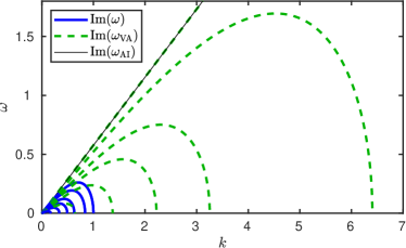
Figure 1: (Color online) Stability spectrum for the DSS. Depicted is the eigenfrequency $\omega$ as a function of the transverse wavenumber $k$ for $\mu=1$. The solid blue line depicts the unstable modes from full NLS numerics corresponding to the imaginary part of $\omega$. The VA prediction of Eq. (14) is depicted by the green dashed curves while the AI prediction (15) is depicted by the thin black line. The different curves represent different stripe velocities $\eta$ corresponding, from top to bottom, to $\eta=0$, 0.4, 0.6, 0.7, 0.8, and 0.9.

Let us now study the (linear) stability for the reduced VA PDE system of Eqs. (10) and (11). To this end, we linearize the system around the equilibrium configuration $A=\eta$ and $X=0$ by considering $A=\eta+a$ and $X=\eta t+\xi$ for $a,\xi\ll 1$ to find:

$$a_{t} = \alpha\frac{u_{0}^{2}-\eta^{2}}{3}\xi_{yy},$$ (12)

$$\xi_{t} = a-\frac{\alpha}{36}(\pi^{2}-6)\frac{\eta^{2}}{(u_{0}^{2}-\eta^{2})^{2}}a_{yy}.$$ (13)

Linear stability of plane waves $\left[a(y,t),\xi(y,t)\right]=\left[a_{0}e^{\mathrm{i}(ky-\omega t)},b_{0}e^{\mathrm{i}(ky-\omega t)}\right]$ the dispersion relation:

$$\omega^{2}=\frac{\eta^{2}-u_{0}^{2}}{3}k^{2}\left[1+\frac{\alpha}{36}(\pi^{2}-6)\frac{\eta^{2}}{(u_{0}^{2}-\eta^{2})^{2}}k^{2}\right].$$ (14)

As depicted in Fig. 1 (see green dashed curves), Eq. (14) describes a dispersion relation $\omega=\omega(k)$ that has qualitatively the correct shape when compared to the stability of the full (original) NLS model (1) (see solid curves), obtained numerically. However, we note that, despite having the correct trend, the dispersion curves fail to accurately capture quantitatively the actual growth rates and wavenumber cutoffs for stability (i.e., wavenumbers $k_{c}$ such that $\omega(k_{c})=0$). This qualitative shape improves on the previous reduced description for the dynamics of DSSs based on the AI assumption aipaper ; aipaper2 ; aipaper3 . The reduced AI PDE for DSSs yields, for $\eta=0$, the following (linear) dispersion relation aipaper3 :

$$\omega^{2}=-\frac{u_{0}^{2}}{3}k^{2},$$ (15)

which simply predicts a linear growth (see thin black line in Fig. 1) of the instability rates as the wavenumber increases. Therefore, inspired by the correct qualitative shape of the dispersion curves from the VA reduced model, we now propose a modification of the VA model so as to also quantitatively match more adequately the dispersion curves.

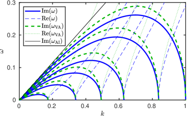
Figure 2: (Color online) Stability spectrum for the DSS. Depicted is the eigenfrequency $\omega$ as a function of the transverse wavenumber $k$ for $\mu=1$. Same notation and layout as in Fig. 1 where now the thick green dashed line corresponds to the improved VA prediction of Eq. (22). For completeness we also show the real part of the eigenfrequency for the full NLS system (thin blue dashed curves) and the improved VA (green dotted line).

In order to modify the VA approach to appropriately capture the correct instability growth rates, we choose to modify the reduced VA PDEs so to match the correct wavenumber cutoffs $k_{c}$. We thus amend our Lagrangian (7) by considering the phenomenological variant:

$$L_{y} = 2X_{t}\left(-AB+u_{0}^{2}\arctan{\frac{B}{A}}\right)-\frac{4}{3}B^{3}$$ (16)

$$+\alpha\frac{2B^{3}}{A^{2}h(B)}B_{y}^{2}+\frac{2\alpha}{3}B^{3}X_{y}^{2},$$

where we have introduced the function

$$h(B)=B^{2}-2+2\sqrt{B^{4}-B^{2}+1}$$ (17)

so as to match the wavenumber cutoffs $k_{c}$ obtained from an asymptotic approximation to the linear stability problem KT . With this modification, the improved equations of motion (for the elliptic case $\alpha=-1$) for a DSS yields:

$$A_{t} = -\frac{B^{2}}{3}X_{yy}+AA_{y}X_{y},$$ (18)

$$X_{t} = A+\frac{A}{2}X_{y}^{2}+\frac{A_{yy}}{h}+\frac{AA_{y}^{2}}{2B^{2}}\left[B\frac{h^{\prime}}{h^{2}}-\frac{1}{h}\right].$$ (19)

The corresponding linearization for this new reduced PDE model yields:

$$a_{t} = -\frac{u_{0}^{2}-\eta^{2}}{3}\xi_{yy},$$ (20)

$$\xi_{t} = a+\frac{1}{h(\sqrt{u_{0}^{2}-\eta^{2}})}a_{yy},$$ (21)

which in turn yields the linear dispersion

$$\omega^{2} = \frac{\eta^{2}-u_{0}^{2}}{3}k^{2}\left[1-\frac{k^{2}}{h(\sqrt{u_{0}^{2}-\eta^{2}})}\right].$$ (22)

By construction, Eq. (22) captures, as expected, the critical wave numbers $k_{c}^{2}={h(\sqrt{u_{0}^{2}-\eta^{2}})}$ where instability for $k<k_{c}$ changes to stability for $k>k_{c}$ for all values of the propagation velocity $A=\eta$, see Fig. 2. Furthermore, as it can be observed from Fig. 2, not only the critical cutoffs $k_{c}$ match, but the maximum growth rates are also well approximated with the improved VA equations. Therefore, we expect that the modified Lagrangian $(\ref{eq14})$, leading to the VA equations (18)-(19), is able to give a good description for the DSS dynamics for all wavenumbers. We will return to this point in Sec. IV, where we will present our numerical comparisons. This is in contrast with the AI approach aipaper ; aipaper2 ; aipaper3 which, by construction, is valid for small wavenumbers and should thus be expected to be more adequate there (as will be again seen in Sec. IV).

III Variational Approach for Two Stripes

In this section we develop a VA approach to follow the interaction of two DSSs akin to what was obtained using the AI approach in Ref. aipaper3 . Consider again the defocusing ($\alpha=-1$) 2D NLS Eq.(1), which, as mentioned before, may be derived from the renormalized (in the $x$-direction) Lagrangian (4)-(5), which we now split as follows:

$$L=\int_{-\infty}^{\infty}L_{y}\,dy=\int_{-\infty}^{\infty}\left(L_{1}+L_{2}+L_{3}\right)dy,$$ (23)

where

$$L_{1} = \frac{\mathrm{i}}{2}\int_{-\infty}^{\infty}\left(u^{*}u_{t}-uu_{t}^{*}\right)\left(1-\frac{u_{0}^{2}}{|u|^{2}}\right)dx,$$ (24)

$$L_{2} = -\frac{1}{2}\int_{-\infty}^{\infty}\left(|u_{x}|^{2}+\left(|u|^{2}-u_{0}^{2}\right)^{2}\right)dx,$$ (25)

$$L_{3} = -\frac{1}{2}\int_{-\infty}^{\infty}|u_{y}|^{2}dx.$$ (26)

In order to variationally follow the 1D two-dark soliton extension of Eq. (3) as two DSSs in 2D, we consider the following 2D symmetric extension by allowing each dark soliton to have its own position and keep a stationary background ($k=0$):

$$u\left(x,y,t\right) = B\left(y,t\right)T_{1}(y,t)T_{2}(y,t)+\mathrm{i}A\left(y,t\right),$$ (27)

where we use the following short-hand definitions:

$$T_{1}(y,t) \equiv \tanh z_{1}\left(y,t\right),$$

$$T_{2}(y,t) \equiv \tanh z_{2}\left(y,t\right),$$

$$z_{1}(y,t) \equiv B\left(y,t\right)\left(x-X_{1}\left(y,t\right)\right),$$

$$z_{2}(y,t) \equiv B\left(y,t\right)\left(x-X_{2}\left(y,t\right)\right),$$

$$S_{1}(y,t) \equiv \operatorname{sech}z_{1}\left(y,t\right),$$

$$S_{2}(y,t) \equiv \operatorname{sech}z_{2}\left(y,t\right),$$

where $X_{1}\left(y,t\right)$ and $X_{2}\left(y,t\right)$ are the spatio-temporal locations of the two DSSs with $X_{1}<X_{2}$. The two-DSS ansatz (27) has an overall background level $B$ and velocity $A$ ($A>0$ representing the two DSSs moving outwards and $A<0$ inwards) where, as for the one DSS case, the relation $A^{2}+B^{2}=u_{0}^{2}=$constant remains valid. It is important to mention here that a more elaborate two DSS ansatz with independent velocities for each dark soliton does not allow for a tractable VA approach (i.e., integrals that can be obtained in closed form in the Lagrangian). Therefore, we restrict our attention to the ansatz (27) that has the drawback of having a common (symmetric) velocity for both dark solitons so that a solution that is not symmetric, namely $\dot{X}_{2}\not=-\dot{X}_{1}$ will eventually tend to a symmetric one ($\dot{X}_{2}=-\dot{X}_{1}$) as time evolves (see Sec. IV for more details).

Let us now perform the VA approach using the two DSS ansatz (27). Letting $\Delta\equiv X_{2}-X_{1}>0$ (i.e., the two dark solitons do not overlap, nor change relative positions) and assuming $B\Delta\gg 1$ (i.e., the two dark solitons are relatively well separated), we have the following useful approximations:

$$T_{1}T_{2} \approx 1+T_{2}-T_{1}-L(x)e^{-2B\Delta},$$ (28)

$$T_{1}S_{2}^{2} \approx S_{2}^{2}-F(x)e^{-2B\Delta},$$ (29)

$$T_{2}S_{1}^{2} \approx -S_{1}^{2}+G(x)e^{-2B\Delta},$$ (30)

$$S_{1}^{2}S_{2}^{2} \approx H(x)e^{-2B\Delta},$$ (31)

where the precise form of the functions $L$, $F$, $G$ and $H$ is not particularly important at this stage as they all contribute to the same order ($e^{-2B\Delta}$) and will all be combined appropriately in the final, explicit results below [cf. Eq. (38) in what follows]. Using this information, we compute:

$$|u|^{2} = u_{0}^{2}-B^{2}\left(S_{1}^{2}+S_{2}^{2}-S_{1}^{2}S_{2}^{2}\right),$$ (32)

$$u_{x} = BD\left(S_{1}^{2}T_{2}+T_{1}S_{2}^{2}\right)$$

$$\frac{\mathrm{i}}{2}\left(u^{*}u_{t}-uu_{t}^{*}\right) = \frac{u_{0}^{2}}{A}B_{t}T_{1}T_{2}+AB\left(z_{2t}S_{2}^{2}-z_{1t}S_{1}^{2}\right)$$ (33)

$$+AB\left(z_{1t}g-z_{2t}f\right)e^{-2D\Delta}.$$

Using the above we can simplify the integrand of $L_{1}$ as:

$$\frac{\mathrm{i}}{2}\left(u^{*}u_{t}-uu_{t}^{*}\right)\left(1-\frac{u_{0}^{2}}{|u|^{2}}\right)$$

$$\approx -\frac{u_{0}^{2}}{A}B^{2}B_{t}\left(\frac{T_{1}T_{2}S_{1}^{2}}{u_{0}^{2}-B^{2}S_{1}^{2}}+\frac{T_{1}T_{2}S_{2}^{2}}{u_{0}^{2}-B^{2}S_{2}^{2}}\right)$$ (34)

$$-AB^{3}\left(z_{2t}\frac{S_{2}^{4}}{u_{0}^{2}-B^{2}S_{2}^{2}}-z_{1t}\frac{S_{1}^{4}}{u_{0}^{2}-B^{2}S_{1}^{2}}\right),$$

where the approximation,

$$\frac{S_{1}^{2}S_{2}^{2}-S_{1}^{2}-S_{2}^{2}}{\frac{u_{0}^{2}}{B^{2}}-S_{1}^{2}-S_{2}^{2}+S_{1}^{2}S_{2}^{2}}$$

$$\approx -\frac{S_{1}^{2}}{\frac{u_{0}^{2}}{B^{2}}-S_{1}^{2}}-\frac{S_{2}^{2}}{\frac{u_{0}^{2}}{B^{2}}-S_{2}^{2}}+R(x)e^{-2D\Delta},$$

has been used with $z_{1t}=\frac{D_{t}}{D}z_{1}-DX_{1t}$ and $z_{2t}=\frac{D_{t}}{D}z_{2}-DX_{2t}$. As it was the case for the functions $L$, $F$, $G$, and $H$ above, the precise form of the function $R$ is not relevant at this stage as it will be combined in the explicit Lagrangian given in Eq. (38) below. We thus get, upon integration,

$$L_{1} \approx 2\Delta_{t}f\left(B\right),$$ (35)

where

$$f\left(B\right)=-AB+u_{0}^{2}\arctan\frac{B}{A}.\\$$

On the other hand for the $L_{2}$ integral, using exact integrations yields:

$$L_{2}=-\frac{8}{3}B^{3}+g\left({B\Delta}\right)B^{3}\approx-\frac{8}{3}B^{3}+16B^{3}e^{-2B\Delta},$$ (36)

where

$$g\left(z\right)\equiv\frac{-16e^{2z}}{\left(e^{2z}\!-\!1\right)^{5}}\left[1+\left(9+12z\right)e^{2z}\!-\!\left(9-12z\right)e^{4z}\!-\!e^{6z}\right].$$

Finally, considering the transverse dependence of $u$, from Eq. (28), we rewrite (27) as $u=B\left[\tanh D(x-X_{2}(y,t))-\tanh D(x-X_{1}(y,t))+1\right]+\mathrm{i}A$. As in the single dark stripe case, assuming that $B$ and $A$ do not depend on $y$, directly but through the relations $D=B$ and $A^{2}+B^{2}=u_{0}^{2}$ for $D=D(y,t)$, yields:

$$u_{y} = B\left[\left(D(x-X_{2})\right)_{y}S_{2}^{2}-\left(D(x-X_{1})\right)_{y}S_{1}^{2}\right],$$

$$|u_{y}|^{2} = B^{2}\left[z_{2y}^{2}S_{2}^{4}+z_{1y}^{2}S_{1}^{4}-2z_{1y}z_{2y}S_{1}^{2}S_{2}^{2}\right].$$

Assuming small and slow displacements, we can safely neglect the cross terms $D_{y}X_{1y}$ and $D_{y}X_{2y}$ from $z_{1y}^{2}$, $z_{2y}^{2}$ and $z_{1y}z_{2y}$ and thus we obtain:

$$\frac{L_{3}}{B^{2}} \approx -\frac{B_{y}^{2}}{B^{3}}\frac{\pi^{2}-6}{9}-\frac{2}{3}B\left(X_{1y}^{2}+X_{2y}^{2}\right)$$ (37)

$$+X_{1y}X_{2y}B^{3}K\left(B\Delta\right),$$

where

$$K\left(z\right) \equiv 4\frac{z\coth z-1}{\sinh^{2}z}.$$

Now, recalling the introduction of the factor $h(B)$ in Eq. (17) to improve the agreement of the growth rates with the numerically observed ones, we finally obtain the effective Lagrangian:

$$L_{y} = 2\Delta_{t}f\left(B\right)-\frac{8}{3}B^{3}+g\left(B\Delta\right)B^{3}-\frac{4B^{3}B_{y}^{2}}{A^{2}h(B)}$$ (38)

$$-\frac{2}{3}B^{3}\left(X_{1y}^{2}+X_{2y}^{2}\right)+X_{1y}X_{2y}B^{3}K\left(B\Delta\right).~{}~{}~{}~{}$$

According to the Euler-Lagrange prescription, taking variations over $X_{1}$, $X_{2}$, and $B$ and recalling that $\Delta\equiv X_{2}-X_{1}$ and $A^{2}+B^{2}=u_{0}^{2}$, yields:

$$A_{t}\!\! = \!\!-\frac{1}{4}B^{3}g^{\prime}+\frac{1}{2}AA_{y}-\frac{1}{6}B^{2}\Delta_{yy}+\frac{1}{4B}AA_{y}K\Delta_{y}+\frac{1}{8}K^{\prime}AA_{y}\Delta\Delta_{y}-\frac{1}{8}K^{\prime}B^{2}\Delta_{y}^{2}-\frac{1}{8}BK\Delta_{yy}-\frac{1}{4}B^{3}K^{\prime}X_{1y}X_{2y},$$ (39)

$$X_{1t}\!\! = \!\!-A-\frac{BA}{4}X_{1}g^{\prime}+\frac{3}{8}Ag+\frac{AA_{y}^{2}}{2B^{2}h}\left(5-\frac{B}{h}h^{\prime}\right)-\frac{A_{yy}}{h}-\frac{A}{4}\left(X_{1y}^{2}+X_{2y}^{2}\right)-\frac{A}{4}X_{1y}X_{2y}X_{1}BK^{\prime}+\frac{3}{8}AKX_{1y}X_{2y},~{}~{}~{}~{}~{}~{}$$ (40)

$$X_{2t}\!\! = \!\!+A-\frac{BA}{4}X_{2}g^{\prime}-\frac{3}{8}Ag-\frac{AA_{y}^{2}}{2B^{2}h}\left(5-\frac{B}{h}h^{\prime}\right)+\frac{A_{yy}}{h}+\frac{A}{4}\left(X_{1y}^{2}+X_{2y}^{2}\right)-\frac{A}{4}X_{1y}X_{2y}X_{2}BK^{\prime}-\frac{3}{8}AKX_{1y}X_{2y}.~{}~{}~{}~{}~{}~{}$$ (41)

Equations (39)–(41) represent one of the main results of this work where the VA methodology has been employed to reduce the full dynamics of two interacting DSSs in two spatial dimensions to these three (1+1)D coupled PDEs. It is interesting to note that, if one starts with a symmetric initial configuration $X_{2}(y,t=0)=-X_{1}(y,t=0)$, given the symmetry of Eqs. (40) and (41), the dynamics preserves this symmetry at all times [i.e., $X_{2}(y,t)=-X_{1}(y,t)$ is an invariant manifold of the dynamics during the evolution] and hence the coupled PDEs can be reduced to solely the equations Eq. (40) for $X_{1}$ and Eq. (39) for $A$.

IV Numerical results

In this section we corroborate that the dynamical reduction, for a single DSS and for two interacting DSSs, obtained through the VA approach is indeed valid under a wide range of initial conditions. Moreover, we compare the VA results with the AI methodology put forward in Refs. aipaper ; aipaper2 ; aipaper3 and showcase where the two display similar results, as well as where the former represents a significant improvement over the latter. It is important to stress that, from now on, we use the improved VA model that includes the $h(B)$ term introduced in Eq. (17). Let us start by considering a single DSS. The DSS is always unstable (snaking instability) to transverse wavenumbers $k$ such that $0\leq k\leq k_{c}$ (see previous section). Therefore, if one considers a spatial domain $(x,y)\in[-L_{x},L_{x}]\times[-L_{y},L_{y}]$, with a DSS aligned in the $y$-direction (i.e., using the same notation as in the previous section), there will always be snaking instability provided that $L_{y}>\pi/k_{c}$. Conversely, if the domain is too small, unstable transverse modes do not “fit” inside the domain and thus the DSS is rendered stable (recall for instance how this property can be used to arrest the instability of DSSs in trapped BECs in Ref. infrared ).

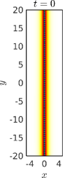
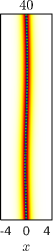
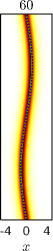
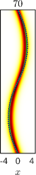
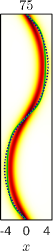
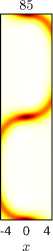
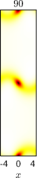
Figure 3: (Color online) Snaking dynamics of the DSS for $\mu=1$ perturbed by the first transverse mode of the computational box. The system is initialized with a stationary DSS perturbed with the $k=1$ transverse mode with amplitude 0.01. Namely, the initial location of the dark soliton at position $y$ is given by $X(y,t=0)=\varepsilon\,\sin(k\pi y/L_{y})$ with $\varepsilon=0.01$ and $k=1$. The modulus of the field, $|u(x,y,t)|$, is plotted in the $(x,y)$ plane at the times indicated. The AI prediction is depicted using the dark blue (black) dotted line while the corresponding improved VA prediction is depicted by the green (gray) solid line. The spatial domain is $(x,y)\in[-L_{x},L_{x}]\times[-L_{y},L_{y}]$ with $L_{x}=L_{y}=20$ (only the region $-5\leq x\leq 5$ is depicted) under a spatial discretization with $\tt{dx}=\tt{dy}=0.2$. See Supplemental Material movie-snake-1 for an animation depicting the corresponding dynamics SupMat .

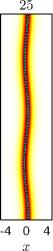
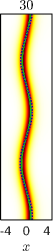
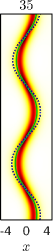
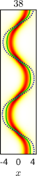
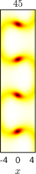
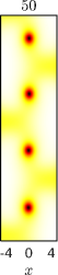
Figure 4: (Color online) Snaking dynamics of the DSS for $\mu=1$ perturbed by the second transverse mode. Same as in Fig. 3 but for $k=2$. See Supplemental Material movie-snake-2 for an animation depicting the corresponding dynamics SupMat .

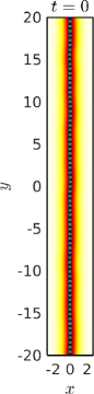
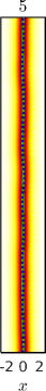
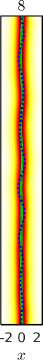
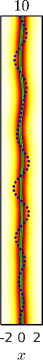
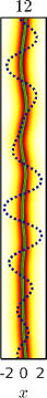
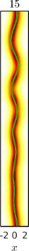
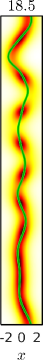
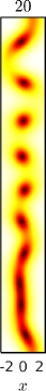
Figure 5: (Color online) Snaking dynamics of the DSS for $\mu=1$ perturbed by a linear combination of the first 10 modes. Same as in Fig. 3 but for a perturbation of the initial position of the dark soliton given by $X(y,t=0)=\sum_{j=1}^{10}\varepsilon_{j}\,\sin[k\pi(y+\varphi_{j})/L_{y}]$ with $\varepsilon_{j}=0.01$, $\varphi_{j}=(j-1)L_{y}\pi/5$, and $k=j$. See Supplemental Material movie-snake-1-10 for an animation depicting the corresponding dynamics SupMat .

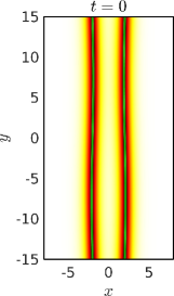
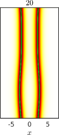
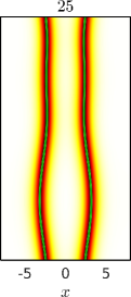
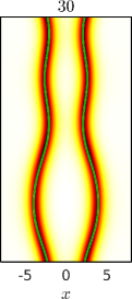
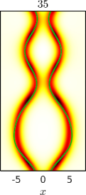
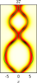
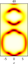
Figure 6: (Color online) Snaking dynamics of two DSSs for $\mu=1$ perturbed by the first transverse mode. The system is initialized with two DSSs at $x_{1}=-2=-x_{2}$ symmetrically perturbed with the $k=1$ transverse mode with amplitude 0.1. Namely, the initial location of each DSSs at position $y$ is given by $-X_{1}(y,t=0)=X_{2}(y,t=0)=x_{0}+\varepsilon\,\sin(k\pi y/L_{y})$ with $x_{0}=2$, $\varepsilon=0.1$ and $k=1$. The modulus of the field, $|u(x,y,t|$, is plotted in the $(x,y)$ plane at the times indicated. The prediction stemming from the improved VA reduced equations (39)–(41) is depicted by the green solid line. The spatial domain is $(x,y)\in[-L_{x},L_{x}]\times[-L_{y},L_{y}]$ with $L_{x}=20$ and $L_{y}=15$. See Supplemental Material movie-2snakes-1 for an animation depicting the corresponding dynamics SupMat .

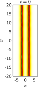
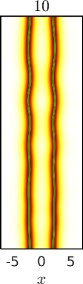
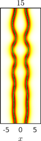
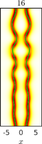
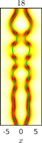
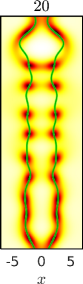
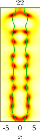
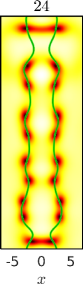
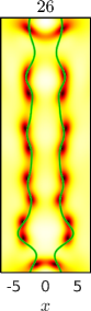
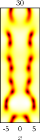
Figure 7: (Color online) Snaking dynamics of two DSSs for $\mu=1$ perturbed by a linear combination of the first 10 modes. Same as in Fig. 6 but for a perturbation of the initial position of the dark solitons given by $-X_{1}(y,t=0)=X_{2}(y,t=0)=x_{0}+\sum_{j=1}^{10}\varepsilon_{j}\,\sin[k\pi(y+\varphi_{j})/L_{y}]$ with $x_{0}=2$, $\varepsilon_{j}=0.01$, $\varphi_{j}=(j-1)L_{y}\pi/5$, and $k=j$. The spatial domain is $(x,y)\in[-L_{x},L_{x}]\times[-L_{y},L_{y}]$ with $L_{x}=L_{y}=20$. See Supplemental Material movie-2snakes-1-10 for an animation depicting the corresponding dynamics.

In order to test the validity of the improved VA approach, we performed a series of simulations for the dynamical evolution of a single DSS under different perturbations using second order finite differencing in space Caplan13a with fourth-order Runge-Kutta with periodic boundary condition along the $y$-direction and mod-squared Dirichlet (MSD) boundary conditions Caplan14 along the $x$-direction in order to avoid any undesired effects from the boundaries. The simulations depicted in Figs. 3–5 are aimed at controllably testing the dynamics of perturbations with different wavenumbers in the domain $L_{x}=L_{y}=20$. In particular, Fig. 3 depicts the dynamics ensuing from an initially stationary [$\eta=A(y,t=0)=0$] DSS that has been perturbed with the longest possible wavelength (satisfying the periodic boundary conditions in the $y$-direction). In addition to testing the VA reduced equations of motion, we also implement the AI methodology put forward in Refs. aipaper ; aipaper2 ; aipaper3 . As it can be seen from the figure, both the improved VA [see the thick green (gray) curves] and the AI [see the dark blue (black) dotted curves] methodologies give a reliable description of the snaking dynamics up to the point where the DSS loses its transverse dark-soliton-like profile as it nucleates vortices of alternate signs at the nodes of the perturbation mode. A few remarks are in order at this point. Firstly, neither the VA nor the AI methods were designed, by construction, to follow the stripe after losing its dark-soliton-like stripe shape. Thus, as DSSs tend to decay into vortex patterns, there will always be a point in time where the VA (or AI) basic assumptions will be violated (most notably the ansatz of a dark solitonic stripe being an accurate descriptor of the full 2D field) and thus the dynamical reduction will no longer be valid. On the other hand, as it can be noticed from Fig. 2, for low wavenumbers pertaining the case of Fig. 3, both VA and AI are able to appropriately predict the correct growth rate of perturbations. However, as one notices from Fig. 2, both VA and AI tend to slightly overestimate the growth rates. This is precisely what it is observed from Fig. Fig. 3 where both VA and AI reductions tend to slightly “run faster” in the dynamical destabilization. Note however, that the VA’s overestimation is slightly smaller than the one obtained through the AI. As we see next, this issue with the AI overestimation will become more acute for larger perturbation wavenumbers.

Figure 4 depicts a similar case as the one depicted in Fig. 3 but for the mode with the second largest wavelength. Again, both the improved VA and AI tend to slightly overestimate the growth rate of the perturbation with the VA approximation being better than the AI one. In order to test a more complex scenario where the essence of the improvement of the theory proposed in this work is most dramatically evident, we perturbed the stationary DSS with a combination of the first 10 modes. The results are depicted in Fig. 5. As it can be observed from the figure, the VA reduction does an excellent job at following the dynamical stabilization of the DSS. On the other hand, as we are now introducing larger wavenumbers, the AI is clearly less accurate (as we expected from its spectral predictions) and tends to considerably overestimate the growth rates. In fact, it can be noticed that the VA approximation is even able to track the full nonlinear dynamics of the DSS up to the point (and even, arguably, slightly beyond, considering e.g. the snapshot at $t=18.5$) where it has broken into a pattern including vortex-antivortex pairs. Furthermore, as the configuration contains larger wavenumbers, the instability sets in faster and, thus, the slight growth rate overestimation provided by the VA is now downplayed over the span of time before the DSS breaks into vortices. This highlights that in a typical scenario where several unstable modes are present, the improved VA will be an excellent reduced description of the full dynamics of single DSSs.

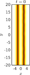
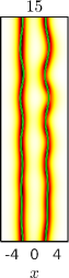
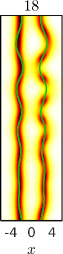
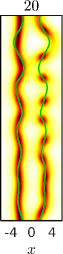
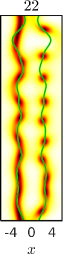
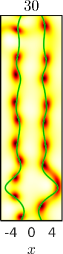
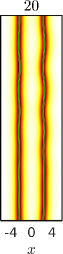
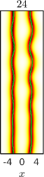
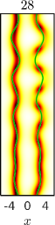
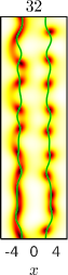
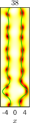
Figure 8: (Color online) Snaking dynamics of two DSSs for $\mu=1$ perturbed by a non-symmetric perturbation where only the right DSS is perturbed. Similar as in Fig. 7 but for an unperturbed left DSS given by $X_{1}(y,t=0)=-x_{0}$ and a right DSS perturbed by $X_{2}(y,t=0)=x_{0}+\sum_{j=1}^{10}\varepsilon_{j}\,\sin[k\pi(y+\varphi_{j})/L_{y}]$ with $x_{0}=2$, $\varphi_{j}=(j-1)L_{y}\pi/5$, and $k=j$ (i.e., same as in Fig. 7), where the perturbation strengths for the right DSS are: $\varepsilon_{j}=0.01$ (top series of panels) and $\varepsilon_{j}=0.001$ (bottom series of panels). Note that although the dynamics for both cases is very similar, the case with the weakest perturbation (see bottom panels) displays a perturbation growth at a slower time scale (contrast the difference in times between the two cases). Importantly also note the deviation induced by the asymmetry between the (by construction symmetric) VA and the full dynamics. See Supplemental Material movie-2snakes-0-0-1-10-A and movie-2snakes-0-0-1-10-B for animations depicting the corresponding dynamics.

We now proceed to test the improved VA prediction for the interaction of two DSSs. Similar to the one DSS case, let us probe both the long wavelength scenario and multiple, mixed mode case. Figure 6 depicts the evolution for two stationary (side-by-side) DSSs symmetrically perturbed by the longest possible wavelength in the provided domain. As the picture shows, the VA is able to track extremely well the DSS dynamics up to the point where the DSSs touch, reconnect, and split into patterns involving vortical structures. It is important to note that we have chosen a configuration where the interactions between the two stripes are quite not trivial. This can be noticed by the fact that the top portions of the DSSs (for $y\approx 8$) initially get closer to each other (due to the individual growth rates of the snaking instability for each DSS) and then repel each other ($t>20$) once the DSS proximity is such that the mutual dark soliton repulsion dominates the dynamics. A more compelling case can be made by testing the VA prediction for the two DSSs by starting with an initial condition containing a non-trivial combination of the first ten modes; see Fig. 7. As for the one DSS case presented in Fig. 5, the two DSS VA reduction is also able to adequately track the two DSSs even well after they break up into individual vortices; see in particular the snapshots between $t=18$ and $t=26$. It is relevant to mention that, as in single DSS case, two DSSs case may also be approximated by the AI methodology aipaper3 . However, one needs to keep in mind that the AI approach is valid for cases containing long wavelengths. Thus, for cases containing shorter wavelengths (larger wavenumbers), as it is particularly the case depicted in Fig. 7, the VA is a very good approximation while the AI will fail in a similar manner akin to the results presented in Fig. 5 for the single DSS.

Finally, for completeness, we briefly study the case where the perturbation on each of the two DSSs is not symmetric. In this case, due to the chosen ansatz (containing a shared velocity term between the two DSSs), the VA dynamics necessary leads, by construction, to a symmetric configuration. Therefore, in principle, one would not expect the VA to give a meaningful prediction for the two DSSs when perturbed asymmetrically. Nonetheless, we tested that for perturbations with small asymmetries the VA does indeed reasonably well at describing the evolution of the two DSSs, despite its obvious shortcoming in that the evolution of the full dynamics is no longer symmetric. As an example, we depict in Fig. 8 a couple of cases where the left DSS is left unperturbed $X_{1}(y,t=0)=-x_{0}$ while the right DSS is perturbed as in the previous numerical examples. In particular, Fig 8 depicts two case where the right soliton position is perturbed by a linear combination of the first ten modes with (weak) strengths of $0.01$ (top series of panels) and $0.001$ (bottom series of panels). As the figure shows, after some transient, the original NLS (1) dynamics evolves such that the left DSS develops undulations (exerted by the right DSS) that are in fact approximately symmetric with respect to the undulations of the right DSS. Therefore, it is not completely surprising that this behavior is, to some extent, followed by the VA as the results in Fig. 8 show.

V Conclusions

In the present work we deployed the VA methodology in order to provide an improved description of the transversely unstable dynamics of single and multiple (two symmetrically perturbed) DSSs in the defocusing two-dimensional nonlinear Schrödinger equation. The method consists of applying the VA to suitable ansätze that consist of one or two DSSs whose transverse position and velocity are functions of time and the transverse spatial variable. In this manner, we are able to reduce the original (2+1)D NLS into two coupled PDEs in (1+1)D for the dark soliton’s position and velocity. It is also important to highlight here that the standard VA is qualitatively adequate, yet quantitatively misses the spectral instability features of the single DSS. In view of that, we have proposed an amended variant of the VA which captures the critical wavenumbers $k_{c}$ of transverse restabilization (for different speeds) and consequently performs quantitatively better over the entire range of wavenumbers. Our numerical results indicate that for short wavenumbers the VA does a slightly better job at predicting the growth rates of perturbations compared to the adiabatic invariant technique developed in Refs. aipaper ; aipaper2 ; aipaper3 . However, it is for perturbations containing larger wavenumbers (including a non-trivial mix for short and long wavenumbers) that the advantage of the VA methodology is more apparent. Specifically, the reduced equations of motion obtained through the VA are able to closely track the dynamics for one and two interacting DSSs. In fact, the reduced VA methodology is not only successful in tracking the DSSs dynamics up to the point where the DSSs break up into vortices; surprisingly, it continues to adequately trace the position of the remnants of the former stripe even for times slightly beyond its destabilization and breakup into vortical structures. Our numerical results suggest that the reduced VA equations constitute a viable methodology for theoretically reducing [to a (1+1)D setting] and numerically closely tracking the dynamics of DSSs over a wide range of dynamical scenarios (i.e., containing a wide range of perturbations from short to long wavelengths ones).

It is worth mentioning that the VA methodology seems not to be tractable for a general two dark soliton ansatz. Therefore, in our presentation we focus on a more specific ansatz where the two dark solitons share velocities and are thus pushing to stay symmetric (each one being the mirror image of the other one). It would be interesting to generalize the results presented herein by a suitable, and tractable, VA (or other) methodology that would be able to successfully track two DSSs for arbitrary positions and velocities. This would allow to not only treat the general two DSSs case, but the general case of $N$ interacting stripes. Of course, there are other directions that are relevant to pursue as well, based on the program that has been recently developed at the level of the adiabatic invariant methodology. Some of them concern ring dark soliton structures, multi-component (e.g. dark-bright) solitonic patterns, as well as three-dimensional states such as planar or spherical solitons. From a theoretical perspective, understanding better how to justify an amendment like the one proposed herein from first principles (that significantly improves the quantitative tracking of the transversely unstable modes) is also an important challenge for future studies.

- (1) B. Denardo, B. Galvin, A. Greenfield, A. Larraza, S. Putterman, and W. Wright, Phys. Rev. Lett. 68, 1730 (1992).
- (2) P. Marquie, J. M. Bilbault, and M. Remoissenet, Phys. Rev. E 49, 828 (1994).
- (3) Yu. S. Kivshar and B. Luther-Davies, Phys. Rep. 298, 81–197 (1998).
- (4) M. Chen, M. A. Tsankov, J. M. Nash, and C. E. Patton, Phys. Rev. Lett. 70, 1707 (1993); B. A. Kalinikos, M. M. Scott, and C. E. Patton, Phys. Rev. Lett. 84, 4697 (2000).
- (5) D. J. Frantzeskakis, J. Phys. A: Math. Theor. 43, 213001 (2010).
- (6) P. G. Kevrekidis, D. J. Frantzeskakis, and R. Carretero-González, The defocusing nonlinear Schrödinger equation: from dark solitons and vortices to vortex rings (SIAM, Philadelphia, 2015).
- (7) A. B. Kozyrev and D. W. van der Weide, J. Phys. D: Appl. Phys. 41, 173001 (2008); Z. Wang, Y. Feng, B. Zhu, J. Zhao, and T. Jiang, J. Appl. Phys. 107, 094907 (2010); L. Q.English, S. G.Wheeler, Y. Shen, G. P.Veldes, N. Whitaker, P. G. Kevrekidis, and D. J.Frantzeskakis, Phys. Lett. A 375, 1242 (2011).
- (8) A. Chabchoub, O. Kimmoun, H. Branger, N. Hoffmann, D. Proment, M. Onorato, and N. Akhmediev, Phys. Rev. Lett. 110, 124101 (2013); A. Chabchoub, O. Kimmoun, H. Branger, C. Kharif, N. Hoffmann, M. Onorato, and N. Akhmediev, Phys. Rev. E 89, 011002(R) (2014).
- (9) C. Chong, F. Li, J. Yang, M. O. Williams, I. G. Kevrekidis, P. G. Kevrekidis, and C. Daraio Phys. Rev. E 89, 032924 (2014).
- (10) R. Heidemann, S. Zhdanov, R. Sütterlin, H. M. Thomas, and G. E. Morfill, Phys. Rev. Lett. 102, 135002 (2009).
- (11) K. G. Lagoudakis, T. Ostatnický, A. V. Kavokin, Y. G. Rubo, R. André, and B. Deveaud-Plédran, Science 326, 974 (2009); G. Grosso, G. Nardin, F. Morier-Genoud, Y. Léger, and B. Deveaud-Plédran, Phys. Rev. Lett. 107, 245301 (2011); V. Goblot, H. S. Nguyen, I. Carusotto, E. Galopin, A. Lemaitre, I. Sagnes, A. Amo, and J. Bloch, Phys. Rev. Lett. 117, 217401 (2016).
- (12) A. Weller, J. P. Ronzheimer, C. Gross, J. Esteve, M. K. Oberthaler, D. J. Frantzeskakis, G. Theocharis, and P. G. Kevrekidis, Phys. Rev. Lett. 101, 130401 (2008).
- (13) G. Theocharis, A. Weller, J. P. Ronzheimer, C. Gross, M. K. Oberthaler, P. G. Kevrekidis, and D. J. Frantzeskakis, Phys. Rev. A 81, 063604 (2010).
- (14) C. Becker, S. Stellmer, P. Soltan-Panahi, S. Dörscher, M. Baumert, E.-M. Richter, J. Kronjäger, K. Bongs, and K. Sengstock, Nature Phys. 4, 496–501 (2008).
- (15) P. Engels and C. Atherton, Phys. Rev. Lett. 99, 160405 (2007).
- (16) P. G. Kevrekidis, G. Theocharis, D. J. Frantzeskakis, and A. Trombettoni, Phys. Rev. A 70, 023602 (2004).
- (17) B. P. Anderson, P. C. Haljan, C. A. Regal, D. L. Feder, L. A. Collins, C. W. Clark, and E. A. Cornell, Phys. Rev. Lett. 86, 2926–2929 (2001).
- (18) I. Shomroni, E. Lahoud, S. Levy and J. Steinhauer, Nat. Phys. 5, 193-197 (2009).
- (19) C. Becker, K. Sengstock, P. Schmelcher, R. Carretero-González, and P. G. Kevrekidis, New J. Phys. 15, 113028 (2013).
- (20) S. Serafini, M. Barbiero, M. Debortoli, S. Donadello, F. Larcher, F. Dalfovo, G. Lamporesi, G. Ferrari, Phys. Rev. Lett. 115, 170402 (2015).
- (21) P. G. Kevrekidis and D. J. Frantzeskakis, Rev. in Phys. 1, 140 (2016).
- (22) T. M. Bersano, V. Gokhroo, M. A. Khamehchi, J. D’Ambroise, D. J. Frantzeskakis, P. Engels, and P. G. Kevrekidis Phys. Rev. Lett. 120, 063202 (2018).
- (23) A. Negretti and C. Henkel, J. Phys. B: At. Mol. Opt. Phys. 37, L385 (2004); A. Negretti, C. Henkel, and K. Mølmer, Phys. Rev. A 78, 023630 (2008).
- (24) M. I. Shaukat, E. V. Castro, and H. Terças, Phys. Rev. A 95, 053618 (2017).
- (25) E. A. Kuznetsov and S. K. Turitsyn, Zh. Eksp. Teor. Fiz. 94, 119–129 (1988) [Sov. Phys. JETP 67, 1583–1588 (1988)].
- (26) Yu. S. Kivshar and D. E. Pelinovsky, Phys. Rep. 331, 117–195 (2000).
- (27) P. G. Kevrekidis, Wenlong Wang, R. Carretero-González, and D. J. Frantzeskakis, Phys. Rev. Lett. 118, 244101 (2017).
- (28) P. G. Kevrekidis, Wenlong Wang, R. Carretero-González, and D. J. Frantzeskakis, Phys. Rev. A 97, 063604 (2018).
- (29) P. G. Kevrekidis, Wenlong Wang, G. Theocharis, D. J. Frantzeskakis, R. Carretero-González, and B. P. Anderson, Dynamics of interacting dark soliton stripes, In press, Phys. Rev. A 97, 063604 (2018).
- (30) Yu. S. Kivshar and X. Yang, Phys. Rev. E 49, 1657–1670 (1994); D. Neshev, A. Dreischuh, V. Kamenov, I. Stefanov, S. Dinev, W. Fliesser, and L. Windholz, Appl. Phys. B 64, 429 (1997); A. Dreischuh, D. Neshev, G. G. Paulus, F. Grasbon, and H. Walther, Phys. Rev. E 66, 066611 (2002).
- (31) Yu. S. Kivshar and W. Królikowski, Optics Comm. 114, 353–362 (1995).
- (32) E. A. Kuznetsov and S. K. Turitsyn. Sov. Phys. JETP 67, 1583–1588 (1988).
- (33) R. M. Caplan and R. Carretero-González. Appl. Num. Math. 71, 24–40 (2013).
- (34) R. M. Caplan and R. Carretero-González. SIAM J. on Sci. Comp. 36, A1–A19 (2014).
- (35) See Supplemental Material at http://link.aps.org/supplemental/xx.xxxx/PhysRevResearch.x.xxxxxx for movies showing the dynamics of the dark soliton stripes.