Port-Hamiltonian modeling of district heating networks

Abstract

This paper provides a first contribution to port-Hamiltonian modeling of district heating networks. By introducing a model hierarchy of flow equations on the network, this work aims at a thermodynamically consistent port-Hamiltonian embedding of the partial differential-algebraic systems. We show that a spatially discretized network model describing the advection of the internal energy density with respect to an underlying incompressible stationary Euler-type hydrodynamics can be considered as a parameter-dependent finite-dimensional port-Hamiltonian system. Moreover, we present an infinite-dimensional port-Hamiltonian formulation for a compressible instationary thermodynamic fluid flow in a pipe. Based on these first promising results, we raise open questions and point out research perspectives concerning structure-preserving discretization, model reduction, and optimization.

1 Introduction

A very important part of a successful energy transition is an increasing supply of renewable energies. However, the power supply through such energies is highly volatile. That is why a balancing of this volatility and more energy efficiency is needed. An important player in this context are district heating networks. They show a high potential to balance the fluctuating supply of renewable energies due to their ability to absorb more or less excess power while keeping the heat supply unchanged. A long-term objective is to strongly increase energy efficiency through the intelligent control of district heating networks. The basis for achieving this goal is the dynamic modeling of the district heating network itself, which is not available in the optimization tools currently used in industry. Such a dynamic modeling would allow for optimization of the fluctuating operating resources, e.g., waste incineration, electric power, or gas. However, as power and heating networks act on different time scales and since their descriptions lead to mathematical problems of high spatial dimension, their coupling for a dynamic simulation that is efficiently realizable involves various mathematical challenges. One possible remedy is a port-Hamiltonian modeling framework: Such an energy-based formulation brings the different scales on a single level, the port-Hamiltonian character is inherited during the coupling of individual systems, and in a port-Hamiltonian system the physical principles (stability, passivity, conservation of energy and momentum) are ideally encoded in the algebraic and geometric structures of the model. Deriving model hierarchies by using adequate Galerkin projection-based techniques for structure-preserving discretization as well as model reduction, and combining them with efficient adaptive optimization strategies opens up a new promising approach to complex application issues.

Against the background of this vision, this paper provides a first contribution to port-Hamiltonian modeling of district heating networks, illustrating the potential for optimization in a case study, and raising open research questions and challenges. Port-Hamiltonian (pH) systems have been elaborately studied in literature lately; see, e.g., BeaMXZ18 ; MehMW18 ; SchJ14 ; SchM18 and the references therein. The standard form appears as

$$\frac{\mathrm{d}{z}}{\mathrm{d}t}=(J-R)\nabla_{z}\mathcal{H}(z)+(B-P)u,\quad y=(B+P)^{T}\nabla_{z}\mathcal{H}(z)+(S+N)u$$ (1a)

with

$$W=W^{T}\geq 0,\quad W=\left[\begin{array}[]{cc}R&P\\ P^{T}&S\end{array}\right].$$ (1d)

The Hamiltonian $\mathcal{H}$ is an energy storage function, $J=-J^{T}$ is the structure matrix describing energy flux among energy storage elements, $R=R^{T}$ is the dissipation matrix, $B\pm P$ are port matrices for energy in- and output, and $S=S^{T}$, $N=-N^{T}$ are matrices associated with the direct feed-through from input $u$ to output $y$. The system satisfies a dissipation inequality, which is an immediate consequence of the positive (semi-)definiteness of the passivity matrix $W$ and also holds even when the coefficient matrices depend on the state $z$ or explicitly on time $t$, or when they are defined as linear operators on infinite-dimensional spaces. Including time-varying state constraints yields a port-Hamiltonian descriptor system of differential-algebraic equations BeaMXZ18 ; MehMW18 ; Sch13 . Port-Hamiltonian partial differential equations on networks (port-Hamiltonian PDAE) are topic in, e.g., a28:egger:2018 for linear damped wave equations or in c47:liljegren-sailer:2019 for nonlinear isothermal Euler equations. The adequate handling of thermal effects is a novelty of this work. Extending the work of BadMBM18 ; BadZ18 , we make use of a thermodynamically consistent generalization of the port-Hamiltonian framework in which the Hamiltonian is combined with an entropy function. The resulting dynamic system consists of a (reversible) Hamiltonian system and a generalized (dissipative) gradient system. Degeneracy conditions ensure that the flows of the two parts do not overlap. Respective pH-models in operator form can be found, e.g., for the Vlasov–Maxwell system in plasma physics in KraH17 ; KraKMS17 , for the Navier–Stokes equations for reactive flows in AltS17 or for finite strain thermoelastodynamics in BetS19 .

The paper is structured as follows. Starting with the description of a district heating network as a connected and directed graph in Sect. 2, we present models associated to the arcs for the pipelines, consumers, and the depot of the network operator that are coupled with respect to conservation of mass and energy as well as continuity of pressure at the network’s nodes. We especially introduce a hierarchy of pipe models ranging from the compressible instationary Navier–Stokes equations for a thermodynamic fluid flow to an advection equation for the internal energy density coupled with incompressible stationary Euler-like equations for the hydrodynamics. Focusing on the latter, we show that the associated spatially discretized network model can be embedded into a family of parameter-dependent standard port-Hamiltonian systems in Sect. 3 and numerically explore the network’s behavior in Sect. 4. In a study on operating the heating network with respect to the avoidance of power peaks in the feed-in, we particularly reveal the potential for optimization. In view of the other pipe models, a generalization of the port-Hamiltonian framework to cover the dissipative thermal effects is necessary. In Sect. 5 we develop an infinite-dimensional thermodynamically consistent port-Hamiltonian formulation for the one-dimensional partial differential equations of a compressible instationary turbulent pipe flow. From this, we raise open research questions and perspectives concerning structure-preserving discretization, model reduction, and optimization in Sect. 6.

2 Network modeling

Figure 1: A schematic district heating network: Foreflow arcs are plotted in solid black, backflow arcs in dashed black, consumers (households) in dotted blue, and the depot in dash-dotted red.

The district heating network is modeled by a connected and directed graph ${G}=({N},{A})$ with node set $N$ and arc set $A$. This graph consists of (i) a foreflow part, which provides the consumers with hot water; (ii) consumers, that obtain power via heat exchangers; (iii) a backflow part, which transports the cooled water back to the depot; and (iv) the depot, where the heating of the cooled water takes place; see Fig. 1 for a schematic illustration. The nodes ${N}={N}_{\text{ff}}\cup{N}_{\text{bf}}$ are the disjoint union of nodes ${N}_{\text{ff}}$ of the foreflow part and nodes ${N}_{\text{bf}}$ of the backflow part of the network. The arcs ${A}={A}_{\text{ff}}\cup{A}_{\text{bf}}\cup{A}_{\text{c}}\cup\{a_{\text{d}}\}$ are divided into foreflow arcs ${A}_{\text{ff}}$, backflow arcs ${A}_{\text{bf}}$, consumer arcs ${A}_{\text{c}}$, and the depot arc $a_{\text{d}}$ of the district heating network operator. The set of pipelines is thus given by ${A}_{\text{p}}={A}_{\text{ff}}\cup{A}_{\text{bf}}$.

In the following we introduce a model hierarchy for the flow in a single pipe (cf. Fig. 2) and afterward discuss the nodal coupling conditions for the network. Models for consumers (households) and the depot yield the closure conditions for the modeling of the network.

2.1 Model hierarchy for pipe flow

Let $a\in{A}_{\text{p}}$ be a pipe. Starting point for the modeling of the flow in a pipe are the cross-sectionally averaged one-dimensional instationary compressible Navier–Stokes equations for a thermodynamic fluid flow Schlichting06 . We assume that the pipe is cylindrically shaped, that it has constant circular cross-sections, and that the flow quantities are only varying along the cylinder axis. Consider $(x,t)\in(0,\ell)\times(t_{0},t_{\mathrm{end}}]\subseteq\mathbb{R}^{2}$ with pipe length $\ell$ as well as start and end time $t_{0}$, $t_{\text{end}}>0$. Mass density, velocity, and internal energy density, i.e., $\rho,v,e:(0,\ell)\times(t_{0},t_{\mathrm{end}}]\rightarrow\mathbb{R}$, are then described by the balance equations

$$\begin{split}0&=\partial_{t}\rho+\partial_{x}(\rho v),\\ 0&=\partial_{t}(\rho v)+\partial_{x}(\rho v^{2})+\partial_{x}p+\frac{\lambda}{2d}\rho|v|v+\rho g\partial_{x}h,\\ 0&=\partial_{t}e+\partial_{x}(ev)+p\partial_{x}v-\frac{\lambda}{2d}\rho|v|v^{2}+\frac{4k_{\mathrm{w}}}{d}(T-\vartheta).\end{split}$$ (2)

Pressure and temperature, i.e., $p,T:(0,\ell)\times(t_{0},t_{\mathrm{end}}]\rightarrow\mathbb{R}$, are determined by respective state equations. In the momentum balance the frictional forces with friction factor $\lambda$ and pipe diameter $d$ come from the three-dimensional surface conditions on the pipe walls, the outer forces arise from gravity with gravitational acceleration $g$ and pipe level $h$ (with constant pipe slope $\partial_{x}h$). The energy exchange with the outer surrounding is modeled in terms of the pipe’s heat transmission coefficient $k_{\mathrm{w}}$ and the outer ground temperature $\vartheta$. System (2) are (Euler-like) non-linear hyperbolic partial differential equations of first order for a turbulent pipe flow.

The hot water in the pipe is under such a high pressure that it does not turn into steam. Thus, the transition to the incompressible limit of (2) makes sense, yielding the following partial differential-algebraic system for velocity $v$ and internal energy density $e$, where the pressure $p$ acts as a Lagrange multiplier to the incompressibility constraint:

$$\begin{split}0&=\partial_{x}v,\\ 0&=\partial_{t}v+\frac{1}{\rho}\partial_{x}p+\frac{\lambda}{2d}|v|v+g\partial_{x}h,\\ 0&=\partial_{t}e+v\partial_{x}e-\frac{\lambda}{2d}\rho|v|v^{2}+\frac{4k_{\mathrm{w}}}{d}(T-\vartheta).\end{split}$$ (3)

The system is supplemented with state equations for density $\rho$ and temperature $T$. Note that the energy term due to friction is negligibly small in this case and can be omitted.

Since the hydrodynamic and thermal effects act on different time scales, System (3) may be simplified even further by setting $\partial_{t}v=0$, i.e.,

$$\begin{split}0&=\partial_{x}v,\\ 0&=\partial_{x}p+\frac{\lambda}{2d}\rho|v|v+\rho g\partial_{x}h,\\ 0&=\partial_{t}e+v\partial_{x}e+\frac{4k_{\mathrm{w}}}{d}(T-\vartheta),\end{split}$$ (4)

again supplemented with state equations for $\rho$, $T$. System (4) describes the heat transport in the pipe where flow velocity and pressure act as Lagrange multipliers to the stationary hydrodynamic equations. However, the flow field is not stationary at all because of the time-dependent closure (boundary) conditions (at households and the depot). In the presented model hierarchy one might even go a step further and ignore the term concerning the heat transition with the outer surrounding of the pipe, i.e., $4k_{\mathrm{w}}(T-\vartheta)/d=0$, when studying the overall network behavior caused by different operation of the depot; see Sect. 3 and Sect. 4.

Figure 2: Hierarchy of pipe flow models

State equations and material models

In the pressure and temperature regime being relevant for operating district heating networks, we model the material properties of water by polynomials depending exclusively on the internal energy density, and not on the pressure. The relations for temperature $T$, mass density $\rho$, and kinematic viscosity $\bar{\nu}$ summarized in Table 1 are based on a fitting of data taken from the NIST Chemistry WebBook nist16 . The relative error of the approximation is of order $O(10^{-3})$, which is slightly higher than the error $O($5\text{\times}{10}^{-4}$)$ we observe due to neglecting the pressure dependence. The quadratic state equation for the temperature allows a simple conversion between $e$ and $T$, which is necessary since closure conditions (households, depot) are usually stated in terms of $T$; cf. Sect. 2.3. Obviously, $e_{\star}(T_{\star})=0.5\,T_{2}^{-1}(-T_{1}+(T_{1}^{2}-4T_{2}(T_{0}-T_{\star}))^{1/2})$ holds for $T_{\star}(e_{\star})=\sum_{i=0}^{2}T_{i}e_{\star}^{i}$, $e_{\star}\geq 0$.

Table 1: Material properties of water as functions of the internal energy density $z(e)=z_{0}\,z_{\star}(e/e_{0})$, $z\in\{T,\rho,\bar{\nu}\}$, where $z_{\star}$ denotes the dimensionless quantity scaled with the reference value $z_{0}$; in particular $e_{\star}=e/e_{0}$ with $e_{0}=10^{9}\,$\mathrm{J}\text{\,}{\mathrm{m}}^{-3}$$. The stated relative errors of the underlying polynomial approximation hold in the regime $e\in[0.2,0.5]$ $\mathrm{GJ}\text{\,}{\mathrm{m}}^{-3}$ and $p\in[5,25]$ $\mathrm{bar}$, implying $T\in[50,130]$ $\mathrm{\SIUnitSymbolCelsius}$.

Reference	Material model	Rel. error
$T_{0}=1$ $\mathrm{\SIUnitSymbolCelsius}$	$T_{\star}(e_{\star})=59.2453\,e_{\star}^{2}+220.536\,e_{\star}+1.93729$	$1.2\text{\times}{10}^{-3}$
$\rho_{0}=10^{3}$ $\mathrm{kg}\text{\,}{\mathrm{m}}^{-3}$	$\rho_{\star}(e_{\star})=-0.208084\,e_{\star}^{2}-0.025576\,e_{\star}+1.00280$	$6.0\text{\times}{10}^{-4}$
$\bar{\nu}_{0}=10^{-6}$ ${\mathrm{m}}^{2}\text{\,}{\mathrm{s}}^{-1}$	$\bar{\nu}_{\star}(e_{\star})=11.9285\,e_{\star}^{4}-22.8079\,e_{\star}^{3}+17.6559\,e_{\star}^{2}-7.00355\,e_{\star}+1.42624$	$9.9\text{\times}{10}^{-4}$

Remark 1

Alternatively to the specific data-driven approach, the state equations can be certainly also deduced more rigorously from thermodynamic laws. A thermodynamic fluid flow described by (2) satisfies the entropy balance for $s:(0,\ell)\times(t_{0},t_{\mathrm{end}}]\rightarrow\mathbb{R}$, i.e.,

$$0=\partial_{t}s+\partial_{x}(sv)-\frac{\lambda}{2d}\frac{1}{T}\rho|v|v^{2}+\frac{4k_{\mathrm{w}}}{d}\frac{1}{T}(T-\vartheta).$$

Considering the entropy as a function of mass density and internal energy density, $s=s(\rho,e)$, yields the Gibbs identities which can be used as state equations for pressure $p$ and temperature $T$, i.e.,

$$\partial_{\rho}s=-(\rho T)^{-1}(e+p-Ts),\quad\partial_{e}s=T^{-1}.$$

Pipe-related models

The pipe flow is mainly driven in a turbulent regime, i.e., with Reynolds number $\mathrm{Re}>10^{3}$. Thus, the pipe friction factor $\lambda$ can be described by the Colebrook–White equation in terms of the Reynolds number $\mathrm{Re}$ and the ratio of pipe roughness and diameter $k_{\mathrm{r}}/d$,

$$\frac{1}{\sqrt{\lambda}}(v,e)=-2\,\log_{10}\left(\frac{2.52}{\mathrm{Re}(v,e)\,\sqrt{\lambda}(v,e)}+\frac{1}{3.71}\frac{k_{\mathrm{r}}}{d}\right),\quad\mathrm{Re}(v,e)=\frac{|v|\,d}{\bar{\nu}(e)}.$$

The model is used for technically rough pipes. Its limit behavior corresponds to the relation by Prandtl and Karman for a hydraulically smooth pipe, i.e., $1/{\sqrt{\lambda}}=2\log_{10}(\mathrm{Re}\sqrt{\lambda})-0.8$ for $k_{\mathrm{r}}/d\rightarrow 0$, and to the relation by Prandtl, Karman, and Nikuradse for a completely rough pipe, i.e., $1/{\sqrt{\lambda}}=1.14-2\log_{10}(k_{\mathrm{r}}/d)$ for $\mathrm{Re}\rightarrow\infty$, Shashi15 . The underlying root finding problem for $\lambda$ can be solved using the Lambert W-function; see clamond2009efficient . However, in view of the computational effort it can also be reasonable to consider a fixed constant Reynolds number for the pipe as further simplification.

The pipe quantities – length $\ell$, diameter $d$, slope $\partial_{x}h$, roughness $k_{\mathrm{r}}$, and heat transmission coefficient $k_{\mathrm{w}}$ – are assumed to be constant in the pipe model. Moreover, note that in this work we also consider the outer ground temperature $\vartheta$ as constant, which will play a role for our port-Hamiltonian formulation of (2) in Sect. 5 .

2.2 Nodal coupling conditions

For the network modeling it is convenient to use the following standard notation. Quantities related to an arc $a=(m,n)\in{A}$, $m,n\in{N}$, are marked with the subscript $a$, quantities associated to a node $n\in{N}$ with the subscript $n$. For a node $n\in{N}$, let $\delta^{\text{in}}_{n}$, $\delta^{\text{out}}_{n}$ be the sets of all topological ingoing and outgoing arcs, i.e.,

$$\delta^{\text{in}}_{n}=\{a\in{A}\colon\exists m\text{ with }a=(m,n)\},\quad\delta^{\text{out}}_{n}=\{a\in{A}\colon\exists m\text{ with }a=(n,m)\},$$

and let $\mathcal{I}_{n}(t)$, $\mathcal{O}_{n}(t)$, $t\in[t_{0},t_{\text{end}}]$, be the sets of all flow-specific ingoing and outgoing arcs,

$$\mathcal{I}_{n}(t) =\{a\in\delta^{\text{in}}_{n}\colon q_{a}(\ell_{a},t)\geq 0\}\cup\{a\in\delta^{\text{out}}_{n}\colon q_{a}(0,t)\leq 0\},$$

$$\mathcal{O}_{n}(t) =\{a\in\delta^{\text{in}}_{n}\colon q_{a}(\ell_{a},t)<0\}\cup\{a\in\delta^{\text{out}}_{n}\colon q_{a}(0,t)>0\};$$

see, e.g., Geissler_et_al:2015 ; Geissler_et_al:2018 ; Hante_Schmidt:2019 where a similar notation is used in the context of gas networks. Note that the sets $\mathcal{I}_{n}(t)$, $\mathcal{O}_{n}(t)$ depend on the flow $q_{a}$, $a\in A$, in the network, which is not known a priori.

The coupling conditions we require for the network ensure the conservation of mass and energy as well as the continuity of pressure at every node $n\in{N}$ and for all time $t\in[t_{0},t_{\text{end}}]$, i.e.,

$$\sum_{a\in\delta^{\text{in}}_{n}}q_{a}(\ell_{a},t) =\sum_{a\in\delta^{\text{out}}_{n}}q_{a}(0,t),$$ (5a)

$$\sum_{a\in\delta^{\text{in}}_{n}}\hat{q}_{a}(\ell_{a},t)e_{a}(\ell_{a},t) =\sum_{a\in\delta^{\text{out}}_{n}}\hat{q}_{a}(0,t)e_{a}(0,t), \,e_{a}(0,t)=e_{n}(t),\,\,\,\,a\in\mathcal{O}_{n}(t),$$ (5b)

$$p_{a}(\ell_{a},t) =p_{n}(t),\,\,\,a\in\delta^{\text{in}}_{n}, p_{a}(0,t)=p_{n}(t),\,\,\,a\in\delta^{\text{out}}_{n}.$$ (5c)

Here, $q_{a}$ and $\hat{q}_{a}$ denote the mass flow and the volumetric flow in pipe $a$, respectively. They scale with the mass density, i.e., $q_{a}=\rho_{a}v_{a}\varsigma_{a}$ and $\hat{q}_{a}=q_{a}/\rho_{a}$, where $\varsigma_{a}=d^{2}_{a}\pi/4$ is the cross-sectional area of the pipe. In case of incompressibility, it holds that $\hat{q}_{a}(x,t)=\hat{q}_{a}(t)$ is constant along the pipe. The functions $e_{n}$ and $p_{n}$ are auxiliary variables describing internal energy density and pressure at node $n$. Note that the second condition in (5b), namely that the out-flowing energy densities are identical in all (flow-specific outgoing) pipes, rests upon the assumption of instant mixing of the in-flowing energy densities.

2.3 Households, depot, and operational constraints

The network modeling is closed by models for the consumers (households) and the depot of the network operator. Quantities associated to the arc $a$ at node $n$ are indicated by the subscript ${a:n}$.

For the consumer at $a=(m,n)\in{A}_{\text{c}}$, where the nodes $m$ and $n$ belong to the foreflow and backflow part of the network, respectively (cf. Fig. 1), the following conditions are posed for $t\in[t_{0},t_{\text{end}}]$,

$$P_{a}(t) =\hat{q}_{a}(t)\Delta e_{a}(t), v_{a}(t) \geq 0, \Delta e_{a}(t) =e_{a:m}(t)-e_{a:n}(t),$$ (6a)

$$T_{a:n}(t) =T^{\text{bf}}, T_{a:m}(t) \in[T^{\text{ff}}_{-},T^{\text{ff}}_{+}], T_{a:m}(t)-T_{a:n}(t) \leq\Delta T^{\text{c}},$$ (6b)

$$p_{a:n}(t) \in[p^{\text{bf}}_{-},p^{\text{bf}}_{+}], p_{a:m}(t) \in[p^{\text{ff}}_{-},p^{\text{ff}}_{+}], p_{a:m}(t)-p_{a:n}(t) \in[\Delta p^{\text{c}}_{-},\Delta p^{\text{c}}_{+}].$$ (6c)

The prescribed power consumption $P_{a}$ of the household is realized by the product of the energy density difference at the arc and the volumetric flow in (6a). Moreover, the underlying flow velocity has a pre-specified direction. The consumer’s outflow temperature is set to be equal to the contractually agreed temperature $T^{\text{bf}}$. Moreover, the operational constraints ensure a certain temperature range at each consumption point and define a maximal temperature difference between foreflow and backflow part of the consumers. In addition, minimal and maximal values for the pressure level at both backflow and foreflow part of the consumer arcs are prescribed. Finally, the pressure difference between foreflow and backflow part is bounded.

The depot $a_{\text{d}}=(m,n)$ for operating the district heating network is modeled by the following conditions for $t\in[t_{0},t_{\text{end}}]$:

$$e_{a_{\text{d}}:n}(t) =u^{\text{e}}(t),\quad T_{a_{\text{d}}:n}(t)\leq T^{\text{net}},\hskip 62.59596ptv_{a_{\text{d}}}(t)\geq 0,$$ (7a)

$$p_{a_{\text{d}}:m}(t) =u^{\text{p}}(t),\quad p_{a_{\text{d}}:n}(t)=p_{a_{\text{d}}:m}(t)+u^{\Delta\text{p}}(t).$$ (7b)

Here, $u^{\text{p}}$ prescribes the so-called stagnation pressure of the network and $u^{\Delta\text{p}}$ is the realized pressure increase at the depot. The energy density injected at the depot to the foreflow part of the network is denoted by $u^{\text{e}}$. The resulting temperature is bounded above by $T^{\text{net}}$, which also acts as temperature limit for all network nodes.

In addition to the operational constraints in (6) and (7), the pressure in all network nodes is bounded, i.e., $p_{n}(t)\leq p^{\text{net}}$ for $n\in{N}$ and $t\in[t_{0},t_{\text{end}}]$.

3 Port-Hamiltonian formulation of a semi-discrete network model

In this section we present a spatially semi-discrete model variant for the district heating network and discuss its formulation in the port-Hamiltonian context. Making use of the different hydrodynamic and thermal time scales, a finite volume upwind discretization yields a port-Hamiltonian descriptor system for the internal energy density, in which the solenoidal flow field acts as a time-varying parameter.

We describe the network by means of the following partial differential-algebraic system for $t\in[t_{0},t_{\text{end}}]$,

$$\partial_{t}e_{a} =-v_{a}\partial_{x}e_{a}, a\in{A}_{\text{p}},$$ (8a)

$$e_{a}(0,t) =e_{n}(t), a\in\mathcal{O}_{n}(t),\qquad\sum_{a\in\delta^{\text{in}}_{n}}\hat{q}_{a}e_{a}(\ell_{a},t)=\sum_{a\in\delta^{\text{out}}_{n}}\hat{q}_{a}e_{a}(0,t),\quad n\in{N},$$ (8b)

$$e_{a:n}(t) =e^{\text{bf}}, a\in{A}_{\text{c}},$$ (8c)

$$e_{a:n}(t) =u^{\text{e}}(t), a=a_{\text{d}},$$ (8d)

$$g(e,v,p) =0.$$ (8e)

This system results from the incompressible pipe model in (4) and neglecting the cooling term in the energy balance (i.e., $k_{\mathrm{w}}=0$). Here, the condition on the backflow temperature for the consumers is expressed in terms of the internal energy density, cf., $e^{\text{bf}}=e(T^{\text{bf}})$ in (8c). In the formulation we use the separation of thermal and hydrodynamic effects and state the temporal advection of the internal energy density with respect to the algebraic equations covering the hydrodynamics. So, $g(e,v,p)=0$ in (8e) contains the hydrodynamic pipe equations, the pressure continuity at the nodes (5c), the condition on the households’ power consumption (6a), the pressure conditions at the depot (7b), and the conservation of volume

$$\sum_{b\in\delta^{\text{in}}_{n}}\hat{q}_{b}(t)=\sum_{a\in\delta^{\text{out}}_{n}}\hat{q}_{a}(t),\quad n\in{N}.$$ (9)

Considering the volume balance (9) instead of the mass balance (5a) is very convenient in the incompressible setting, since the velocity field and hence the induced volumetric flow are constant along a pipe. Moreover, this description naturally fits the numerical method of finite volumes.

For the spatial discretization of the hyperbolic-like system (8) we apply a classical finite volume upwind scheme leveque_numerical_2008 . Let $\alpha\in{A}_{\text{p}}$, $\alpha\in\mathcal{O}_{n}(t_{0})$, $n\in{N}$, and consider an equidistant mesh of cell size $\Delta x_{\alpha}$, then

$$\frac{\mathrm{d}}{\mathrm{d}t}e_{\alpha,\beta} =-\frac{v_{\alpha}}{\Delta x_{\alpha}}(e_{\alpha,\beta}-e_{\alpha,\beta-1}),\quad\beta\in V_{\alpha},$$

$$e_{\alpha,0} =e_{n},\quad e_{n}=\frac{\sum_{b\in\mathcal{I}_{n}}\hat{q}_{b}\,e_{b,|V_{b}|}}{\sum_{a\in\mathcal{O}_{n}}\hat{q}_{a}},$$

where $e_{\alpha,\beta}$ denotes the internal energy density with respect to the finite volume cell $\beta$ of pipe $\alpha$ with cell index set $V_{\alpha}$. For the first cell ($\beta=1$) we make use of the quantity at the node that results from (8b). We summarize the unknown energy densities in a vector $e=(e_{1},...,e_{\kappa})^{T}$, $e_{f(\alpha,\beta)}=e_{\alpha,\beta}$ by ordering pipe- and cell-wise according to the mapping $f(\alpha,\beta)=\beta+\sum_{k=1}^{\alpha-1}|V_{k}|$, $\alpha\in{A}_{\text{p}}$, $\beta\in V_{\alpha}$, in particular $\kappa=\sum_{\alpha\in{A}_{\text{p}}}|V_{\alpha}|$. Then, a semi-discrete version of the network model (8) is given by the following descriptor system

$$\frac{\mathrm{d}}{\mathrm{d}t}e=A(v)\,e+B(v)\,u,\quad y=Ce,$$ (10)

$$\text{subject to }v=G(e).$$

The system matrices $A(w)\in\mathbb{R}^{\kappa\times\kappa}$ and $B(w)\in\mathbb{R}^{\kappa\times 2}$ can be interpreted as parameter-dependent quantities, where the (vector-valued) parameter $w$ represents a spatially discretized solenoidal volume-preserving velocity field. So,

$$A_{f(\alpha,\beta),f(\mu,\sigma)}(w)=\partial\frac{\mathrm{d}}{\mathrm{d}t}e_{\alpha,\beta}(w)/{\partial e_{\mu,\sigma}}$$

holds. The special velocity field belonging to the hydrodynamic network equations (8e) is formally stated as $v=G(e)$. We assume a setting in which $v$ is time-continuous. In (10) the input $u$ consists of the energy densities $u^{\text{e}}$ injected at the depot into the foreflow part and $e^{\text{bf}}$ returning from the consumers into the backflow part of the network, $u=(u^{\text{e}},e^{\text{bf}})^{T}\in\mathbb{R}^{2}$. The output $y$ typically refers to energy densities in pipes supplying the consumers, implying $C\in\mathbb{R}^{c\times\kappa}$.

Theorem 3.1

Let $w$ be a (spatially discretized) solenoidal volume-preserving time-continuous velocity field. Then, the semi-discrete network model (10) can be embedded into a family of parameter-dependent port-Hamiltonian systems

$$\frac{\mathrm{d}}{\mathrm{d}t}e=(J(w)-R(w))Qe+\tilde{B}(w)\tilde{u},\quad\tilde{y}=\tilde{B}^{T}(w)Qe,$$ (11)

with $\tilde{u}=(u^{T},0,\dotsc,0)^{T}\in\mathbb{R}^{2+c}$ which contains the original outputs as subset.

Remark 2

Theorem 3.1 implies that there exists an energy matrix $Q$ such that

$$QA(w)+A^{T}(w)Q\leq 0$$ (12)

for all solenoidal volume-preserving velocity fields $w$. Thus, the Hamiltonian $\mathcal{H}(e)=e^{T}Qe$ is a Lyapunov function for the parameter-dependent system antoul_approx . The energy matrix $Q$ can be particularly constructed as a diagonal matrix with positive entries, i.e., $Q_{f(\alpha,\beta),f(\alpha,\beta)}=\varsigma_{\alpha}\,\Delta x_{\alpha}$ for $\alpha\in{A}_{\text{p}}$, $\beta\in V_{\alpha}$, where $\varsigma_{\alpha}\,\Delta x_{\alpha}$ is the volume of each discretization cell in pipe $\alpha$.

Note that a change of the flow direction, which might occur in case of cycles, yields a structural modification of the system matrix $A(w)$, but does not affect the stability of the system. However, it might cause a discontinuity in the velocity field such that (10), or (11) respectively, only allows for a weak solution.

Proof (of Theorem 3.1)

Let the positive definite diagonal matrix $Q\in\mathbb{R}^{\kappa\times\kappa}$ with $Q_{f(\alpha,\beta),f(\alpha,\beta)}=\varsigma_{\alpha}\,\Delta x_{\alpha}>0$ be given. Then, we define the matrices $J$ and $R$ by

$$J(w)=\frac{1}{2}(A(w)Q^{-1}-(A(w)Q^{-1})^{T}),\quad R(w)=-\frac{1}{2}(A(w)Q^{-1}+(A(w)Q^{-1})^{T}).$$

Obviously, $A(w)=(J(w)-R(w))Q$ holds. The properties $J=-J^{T}$ and $R=R^{T}$ of port-Hamiltonian system matrices are satisfied by construction for any parameter $w$. The positive semi-definiteness of $R$ follows from the Lyapunov inequality (12). Considering

$$L(w)=QA(w)+A^{T}(w)Q,\quad L_{f(\alpha,\beta),f(\alpha,\beta)}(w)=-2Q_{f(\alpha,\beta),f(\alpha,\beta)}\frac{w_{\alpha}}{\Delta x_{\alpha}}=-2\hat{q}_{\alpha}\leq 0,$$

the volume-preservation of $w$ ensures that the symmetric matrix $L(w)$ is weakly diagonal dominant. Hence, $L(w)$ is negative semi-definite, yielding

$$x^{T}R(w)x=-\frac{1}{2}(Q^{-1}x)^{T}\,L(w)\,(Q^{-1}x)\geq 0\quad\text{for all}\quad x\in\mathbb{R}^{\kappa}.$$

Here, $R(w)$ acts as the passivity matrix since the system has no feed-through term. The port matrix $\tilde{B}(w)\in\mathbb{R}^{\kappa\times 2+c}$ defined by

$$\tilde{B}(w)=[B(w),\,\,(CQ^{-1})^{T}]$$

ensures that the outputs of the network model are contained in the output set of the port-Hamiltonian system, i.e., $\tilde{B}^{T}(w)Q=[B^{T}(w)Q,\,\,C]^{T}$. Finally note that the parameter-dependent port-Hamiltonian system matrices $J(w)$, $R(w)$, and $\tilde{B}(w)$ are continuous in time due to the given time-regularity of the parameter $w$.

Remark 3

We point out that applying the stated framework to the other pipe models presented in Sect. 2.1 is non-trivial. Already the consideration of the cooling term in the energy balance, cf. pipe model (4), which acts dissipative requires a generalization of the port-Hamiltonian description. We refer to Sect. 5 for an infinite-dimensional port-Hamiltonian formulation of the compressible thermodynamic pipe flow (2).

4 Numerical study on network operation

In this section we demonstrate the potential for optimization of district heating networks. Operating the network according to certain exogenously given temporal profiles for the internal energy densities injected at the depot may lead to high amplitudes in the feed-in power. The avoidance of such power peaks in the feed-in prevents that using additional energy sources, such as gas storages, is required for covering the heating demand of the consumers. This is environmental friendly, while saving resources and operational costs.

In the numerical case study we employ a real-world district heating network supplying different streets by means of the port-Hamiltonian semi-discrete network model (10). For the time integration we use an implicit midpoint rule with constant time step $\Delta t$. The topology of the network and the data of the pipelines come from the Technische Werke Ludwigshafen AG; see Fig. 3 and Table 2. For the presented simulation, a time horizon of $50\text{\,}\mathrm{h}$ is studied. The consumption behavior of the households is modeled by standardized profiles used in the operation of district heating networks SLP_BGW for a mean environmental temperature of $3\text{\,}\mathrm{\SIUnitSymbolCelsius}$. The total consumption of all households is $108\text{\,}\mathrm{kW}$ on temporal average and rises up to a maximum of $160\text{\,}\mathrm{kW}$. Given the internal energy density $u^{\text{e}}$ injected at the depot as input, the feed-in power can be considered as the response of the network system, i.e.,

$$P_{\text{in}}=(u^{\text{e}}-e_{a_{\text{d}}:m})\sum_{a\in{A}_{\text{c}}}\hat{q}_{a}.$$

Note that due to the neglect of cooling in (8), $e_{a_{\text{d}}:m}=e(T^{\text{bf}})$ holds, where the backflow temperature at the consumers is fixed here to $T^{\text{bf}}=$60\text{\,}\mathrm{\SIUnitSymbolCelsius}$$.

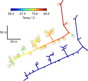
Figure 3: Real-world heating network supplying several streets. The network consists of the foreflow part (top) and the backflow part (bottom), where the households are indicated by circles. The topology has been provided by Technische Werke Ludwigshafen AG, Germany. The color plot visualizes a simulated temperature distribution for a certain time $t^{\star}$, where $T(u^{\text{e}}(t^{\star}))=$84\text{\,}\mathrm{\SIUnitSymbolCelsius}$$. The backflow temperature is constant at $T^{\text{bf}}=$60\text{\,}\mathrm{\SIUnitSymbolCelsius}$$ due to the use of the network model (8) where cooling effects are neglected.

Table 2: Graph-associated outline data for the street network in Fig. 3. The total pipe length of the foreflow part is $835.5\text{\,}\mathrm{m}$ and of the backflow part $837.0\text{\,}\mathrm{m}$.

Pipes $|{A}_{\text{p}}|$	Consumers $|{A}_{\text{c}}|$	Depot	Arcs $|{A}|$	Nodes $|{N}|$	Loops
162	32	1	195	162	2

The traveling time of the heated water from the depot to the consumers (households) allows to choose from different injection profiles, when covering the aggregated heating demand in the network. Figure 4 shows the injected temperature $T(u^{\text{e}})$ and the corresponding feed-in power for two different input profiles. Supplying an almost constant energy density $u^{\text{e}}$ over time yields pronounced power peaks (dashed-dotted red curves). These undesired peaks can be avoided when using an input that is varying in time with respect to the expected consumer demands. For the illustrated improved input, the feed-in power is bounded by $\bar{P}_{\text{in}}=$134\text{\,}\mathrm{kW}$$ (dashed green curves). This promising result asks for a rigorous optimal control of the network in further studies.

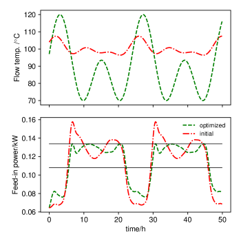
Figure 4: Flow temperature at depot $T(u^{\text{e}})$ (top) and corresponding feed-in power (bottom) over time for two different injection profiles marked in dashed-dotted red and dashed green, $\Delta t=$5\text{\,}\mathrm{min}$$. The upper solid, black line indicates the power threshold $\bar{P}$, the lower one the mean feed-in power over time.

5 Port-Hamiltonian formulation of compressible thermodynamic pipe flow

The adequate handling of thermal effects requires the generalization of the port-Hamiltonian framework by combing the Hamiltonian with an entropy function. In this section we embed the partial differential model (2) for a compressible thermodynamic turbulent pipe flow into the GENERIC-formalism, which has lately been studied in BadMBM18 ; BadZ18 , and present an infinite-dimensional thermodynamically consistent port-Hamiltonian description.

The thermodynamic pipe flow model (2) can be reformulated as a generalized (non-linear) port-Hamiltonian system in operator form for $z=(\rho,M,e)^{T}$, $M=(\rho v)$,

$$\frac{\mathrm{d}z}{\mathrm{d}t} =\left(\mathcal{J}(z)-\mathcal{R}(z)\right)\frac{\delta\mathcal{E}(z)}{\delta z}+\mathcal{B}(z)u(z)\quad \text{in }\mathcal{D}_{z}^{*},$$ (13)

$$y(z) =\mathcal{B}^{*}(z)\frac{\delta\mathcal{E}(z)}{\delta z}\quad \text{in }\mathcal{D}_{u}^{*},$$

where $\mathcal{Z}=\{z\in\mathcal{D}_{z}\,|\,\rho\geq\delta\text{ with }\delta>0\text{ almost everywhere}\}\subset\mathcal{D}_{z}$ denotes the state space with the Sobolev space $\mathcal{D}_{z}=W^{1,3}((0,\ell);\mathbb{R}^{3})$ being a reflexiv Banach space. For $z\in\mathcal{Z}$ the operators $\mathcal{J}(z)[\cdot]$, $\mathcal{R}(z)[\cdot]:\mathcal{D}_{z}\rightarrow\mathcal{D}_{z}^{*}$ are linear and continuous, moreover $\mathcal{J}(z)$ is skew-adjoint and $\mathcal{R}(z)$ is self-adjoint semi-elliptic, i.e., $\langle\varphi,\mathcal{J}(z)\psi\rangle=-\langle\psi,\mathcal{J}(z)\varphi\rangle$ and $\langle\varphi,\mathcal{R}(z)\psi\rangle=\langle\psi,\mathcal{R}(z)\varphi\rangle\geq 0$ for all $\varphi,\psi\in\mathcal{D}_{z}$. The system theoretic input is given by $u(z)\in\mathcal{D}_{u}=L^{q}(\{0,\ell\})$ with linear continuous operator $\mathcal{B}(z)[\cdot]:\mathcal{D}_{u}\rightarrow\mathcal{D}_{z}^{*}$ and dual space $\mathcal{D}_{u}^{*}=L^{p}(\{0,\ell\})$, ${1}/{q}+{1}/{p}=1$. The system theoretic output is denoted by $y(z)$. The form of the energy functional $\mathcal{E}$ and the port-Hamiltonian operators $\mathcal{J}(z)$, $\mathcal{R}(z)$ and $\mathcal{B}(z)[\cdot]$ are derived as follows.

Remark 4

We assume that all relevant mathematical statements hold for an arbitrary but fixed time parameter $t\in(t_{0},t_{\text{end}}]$. The function spaces $\mathcal{D}_{z}$ and $\mathcal{D}_{u}$ associated with the spatial evolution are chosen in an ad-hoc manner, i.e., we assume that the considered fields and functions satisfy certain regularity requirements. A mathematically rigorous justification requires an analytical consideration of the generalized port-Hamiltonian system. The corresponding functional analytical and structural questions are the focus of ongoing work.

Accounting for the thermodynamic behavior of the pipe flow, (13) is composed of a Hamiltonian and a generalized gradient system. This is reflected in the energy functional that is an exergy-like functional consisting of a Hamiltonian and an entropy part, i.e.,

$$\mathcal{E}(z)=\mathcal{H}(z)-\vartheta\mathcal{S}(z),\quad\mathcal{H}(z)=\int_{0}^{\ell}\left(\frac{|M|^{2}}{2\rho}+e+\rho gh\right)\mathrm{d}x,\quad\mathcal{S}(z)=\int_{0}^{\ell}s(\rho,e)\,\mathrm{d}x.$$

where the outer ground temperature $\vartheta$ is assumed to be constant. Introducing the ballistic free energy $H(\rho,e)=e-\vartheta s(\rho,e)$ Feireisl12 , the functional $\mathcal{E}$ and its variational derivatives become

$$\mathcal{E}(z) =\int_{0}^{\ell}\left(\frac{|M|^{2}}{2\rho}+H(\rho,e)+\rho gh\right)\mathrm{d}x$$

$$\frac{\delta\mathcal{E}(z)}{\delta z} =\left(\frac{\delta\mathcal{E}(z)}{\delta\rho},\frac{\delta\mathcal{E}(z)}{\delta M},\frac{\delta\mathcal{E}(z)}{\delta e}\right)^{T}=\left(\left(-\frac{|M|^{2}}{2\rho^{2}}+\frac{\partial H}{\partial\rho}+gh\right),\frac{M}{\rho},\frac{\partial H}{\partial e}\right)^{T}.$$

The port-Hamiltonian operators in (13) are assembled with respect to the (block-) structure of the state $z$. Let $\varphi,\psi\in\mathcal{D}_{z}$ be two block-structured test functions, i.e., $\varphi=(\varphi_{\rho},\varphi_{M},\varphi_{e})^{T}$. Then the skew-adjoint operator $\mathcal{J}(z)$ is given by

$$\mathcal{J}(z)=\left[\begin{array}[]{ccc}0&\mathcal{J}_{\rho,M}(z)&0\\ \mathcal{J}_{M,\rho}(z)&\mathcal{J}_{M,M}(z)&\mathcal{J}_{M,e}(z)\\ 0&\mathcal{J}_{e,M}(z)&0\end{array}\right],$$ (14d)

associated with the bilinear form

$$\langle\varphi,\mathcal{J}(z)\psi\rangle =\langle\varphi_{\rho},\mathcal{J}_{\rho,M}(z)\psi_{M}\rangle+\langle\varphi_{M},\mathcal{J}_{M,\rho}(z)\psi_{\rho}\rangle+\langle\varphi_{M},\mathcal{J}_{M,M}(z)\psi_{M}\rangle$$

$$\quad+\langle\varphi_{M},\mathcal{J}_{M,e}(z)\psi_{e}\rangle+\langle\varphi_{e},\mathcal{J}_{e,M}(z)\psi_{M}\rangle.$$

Its entries are particularly defined by the following relations,

$$\langle\varphi_{\rho},\mathcal{J}_{\rho,M}(z)\psi_{M}\rangle =-\langle\psi_{M},\mathcal{J}_{M,\rho}(z)\varphi_{\rho}\rangle=\int_{0}^{\ell}\rho(\psi_{M}\partial_{x})\varphi_{\rho}\,\mathrm{d}x,$$ (14e)

$$\langle\varphi_{M},\mathcal{J}_{M,M}(z)\psi_{M}\rangle =-\langle\psi_{M},\mathcal{J}_{M,M}(z)\varphi_{M}\rangle=\int_{0}^{\ell}M((\psi_{M}\partial_{x})\varphi_{M}-(\varphi_{M}\partial_{x})\psi_{M})\,\mathrm{d}x,$$ (14f)

$$\langle\varphi_{e},\mathcal{J}_{e,M}(z)\psi_{M}\rangle =-\langle\psi_{M},\mathcal{J}_{M,e}(z)\varphi_{e}\rangle=\int_{0}^{\ell}e(\psi_{M}\partial_{x})\varphi_{e}+(\psi_{M}\partial_{x})(\varphi_{e}p)\,\mathrm{d}x$$ (14g)

that result from the partial derivatives in (2). The self-adjoint semi-elliptic operator $\mathcal{R}(z)$ is composed of two operators that correspond to the friction in the pipe $\mathcal{R}^{\lambda}(z)$ and the temperature loss through the pipe walls $\mathcal{R}^{k_{\mathrm{w}}}(z)$. It is given by

$$\mathcal{R}(z)=\mathcal{R}^{\lambda}(z)+\mathcal{R}^{k_{\mathrm{w}}}(z)=\left[\begin{array}[]{ccc}0&0&0\\ 0&\mathcal{R}^{\lambda}_{M,M}(z)&\mathcal{R}^{\lambda}_{M,e}(z)\\ 0&\mathcal{R}^{\lambda}_{e,M}(z)&\mathcal{R}^{\lambda}_{e,e}(z)+\mathcal{R}^{k_{\mathrm{w}}}_{e,e}(z)\end{array}\right],$$ (15d)

associated with the bilinear form,

$$\langle\varphi,\mathcal{R}(z)\psi\rangle =\langle\varphi_{M},\mathcal{R}^{\lambda}_{M,M}(z)\psi_{M}\rangle+\langle\varphi_{M},\mathcal{R}^{\lambda}_{M,e}(z)\psi_{e}\rangle+\langle\varphi_{e},\mathcal{R}^{\lambda}_{e,M}(z)\psi_{M}\rangle$$

$$\quad+\langle\varphi_{e},(\mathcal{R}^{\lambda}_{e,e}(z)+\mathcal{R}^{k_{\mathrm{w}}}_{e,e}(z))\psi_{e}\rangle.$$

Its entries are

$$\langle\varphi_{M},\mathcal{R}^{\lambda}_{M,M}(z)\psi_{M}\rangle =\int_{0}^{\ell}\varphi_{M}\left(\frac{\lambda}{2d}\frac{T}{\vartheta}\rho|v|\right)\psi_{M}\,\mathrm{d}x,$$ (15e)

$$\langle\varphi_{M},\mathcal{R}^{\lambda}_{M,e}(z)\psi_{e}\rangle=\langle\psi_{e},\mathcal{R}^{\lambda}_{e,M}(z)\varphi_{M}\rangle =\int_{0}^{\ell}-\varphi_{M}\left(\frac{\lambda}{2d}\frac{T}{\vartheta}\rho|v|v\right)\psi_{e}\,\mathrm{d}x,$$ (15f)

$$\langle\varphi_{e},(\mathcal{R}^{\lambda}_{e,e}(z)+\mathcal{R}^{k_{\mathrm{w}}}_{e,e}(z))\psi_{e}\rangle =\int_{0}^{\ell}\varphi_{e}\left(\frac{\lambda}{2d}\frac{T}{\vartheta}\rho|v|v^{2}+\frac{4k_{\mathrm{w}}}{d}T\right)\psi_{e}\,\mathrm{d}x.$$ (15g)

Note that the state dependencies of pressure $p=p(\rho,e)$ and temperature $T=T(\rho,e)$ occurring in (14g) and (15e)-(15g) are prescribed by the state equations, cf. Remark 1. Moreover, $v=M/\rho$ and $\lambda=\lambda(v,e)$ hold for the velocity and the friction factor, respectively. Assuming consistent state equations, e.g., ideal gas law, cf. Remark 5, the operators in (14) and (15) fulfill the non-interacting conditions

$$\mathcal{J}(z)\frac{\delta\mathcal{S}(z)}{\delta z}=0,\quad\quad\mathcal{R}^{\lambda}(z)\frac{\delta\mathcal{H}(z)}{\delta z}=0,$$

which arise in the GENERIC context BadMBM18 ; BadZ18 and ensure that the flows of the Hamiltonian and the gradient system do not overlap. Finally, concerning the system theoretic input and output, the state dependent input is given as $u(z)\in\mathcal{D}_{u}$ by $u(z)=[M/\rho]|^{\ell}_{0}$. Then, the port operator $\mathcal{B}(z)[\cdot]:\mathcal{D}_{u}\rightarrow\mathcal{D}_{z}^{\star}$ is specified through the pairing

$$\langle\varphi,\mathcal{B}(z)u(z)\rangle=-\left.\left[(\varphi_{\rho}\rho+\varphi_{M}M+\varphi_{e}(e+p))\,u(z)\right]\right|_{0}^{\ell},$$

which originates from the boundary terms, when applying partial integration to parts of (2). With the adjoint operator $\mathcal{B}^{*}(z)[\cdot]:\mathcal{D}_{z}\rightarrow\mathcal{D}_{u}^{*}$, i.e., $\langle\varphi,\mathcal{B}(z)u(z)\rangle=\langle\mathcal{B}^{*}(z)\varphi,u(z)\rangle$, the system theoretic output reads

$$y(z)=\mathcal{B}^{*}(z)\frac{\delta\mathcal{E}(z)}{\partial z}=-\left.\left[\frac{|M|^{2}}{2\rho}+p+H(\rho,e)+\rho gh\right]\right|^{\ell}_{0}.$$

Remark 5

In the port-Hamiltonian framework the choice of the state variables in the interplay with the energy functional is crucial for encoding the physical properties in the system operators. Hence, asymptotic simplifications as, e.g., the limit to incompressibility in the hydrodynamics (3), are not straightforward, since they change the underlying equation structure. However, system (13) is well suited when, e.g., dealing with gas networks. Then, it can be closed by using, e.g., the ideal gas law, implying

$$s(\rho,e)=\frac{R}{2}\rho\operatorname{ln}\left(c_{\text{p}}\frac{e^{3}}{\rho^{5}}\right),\quad T(\rho,e)=\frac{2}{3R}\frac{e}{\rho},\quad p(\rho,e)=\frac{2}{3}e,$$

with specific gas constant $R$ and heat capacity $c_{\text{p}}$.

6 Research perspectives

An energy-based port-Hamiltonian framework is very suitable for optimization and control when dealing with subsystems coming from various different physical domains, such as hydraulic, electrical, or mechanical ones, as it occurs when coupling a district heating network with a power grid, a waste incineration plant, or a gas turbine. The formulation is advantageous as it brings different scales on a single level, the port-Hamiltonian character is inherited by the coupling, and the physical properties are directly encoded in the structure of the equations. However, to come up with efficient adaptive optimization strategies based on port-Hamiltonian model hierarchies for complex application issues on district heating networks, there are still many mathematical challenges to be handled.

In this paper we contributed with an infinite-dimensional and thermodynamically consistent formulation for a compressible turbulent pipe flow, which required to set up a (reversible) Hamiltonian system and a generalized (dissipative) gradient system with suitable degeneracy conditions. In particular, the choice of an appropriate energy function was demanding. The asymptotic transition to an incompressible pipe flow is non-trivial in this framework, since it changes the differential-algebraic structure of the equations and hence requires the reconsideration of the variables and the modification of the energy function. In view of structure-preserving discretization and model reduction the use of Galerkin projection-based techniques seems to be promising. However, the choice of the variables and the formulation of the system matrices crucially determine the complexity of the numerics as, e.g., the works CBG2016 ; Egger:2018 ; c47:liljegren-sailer:2019 show. Especially, the handling of the nonlinearities requires adequate complexity-reduction strategies. Interesting to explore are certainly also structure-preserving time-integration schemes, see, e.g., KotL18 ; MorM19 .

In the special case of the presented semi-discrete district heating network model that makes use of the different hydrodynamic and thermal time scales and a suitable finite volume upwind discretization we came up with a finite-dimensional port-Hamiltonian system for the internal energy density where the solenoidal flow field acts a time-varying parameter. This system is employed for model reduction (moment matching) in rein:2019a and for optimal control in rein:2019b .

The application of the port-Hamiltonian modeling framework for coupled systems leads to many promising ideas for the optimization of these systems. Due to the complexity and size of the respective optimization models, a subsystem-specific port-Hamiltonian modeling together with suitable model reduction techniques allows for setting up a coupled model hierarchy for optimization, which paves the way for highly efficient adaptive optimization methods; cf., e.g., MSS18 , where a related approach has shown to be useful for the related field of gas network optimization.

- (1) Altmann, R., Schulze, P.: A port-Hamiltonian formulation of the Navier-Stokes equations for reactive flows. Systems & Control Letters 100, 51–55 (2017). DOI 10.10.16/j.sysconle.2016.12.005
- (2) Antoulas, A.: Approximation of Large-Scale Dynamical Systems. SIAM Publications (2005). DOI 10.1137/1.9780898718713
- (3) Beattie, C., Mehrmann, V., Xu, H., Zwart, H.: Linear port-Hamiltonian descriptor systems. Mathematics of Control, Signals, and Systems 30, 17 (2018). DOI 10.1007/s00498-018-0223-3
- (4) Betsch, P., Schiebl, M.: Energy-momentum-entropy consistent numerical methods for large-strain thermoelasticity relying on the GENERIC formalism. International Journal for Numerical Methods in Engineering 119(12), 1216–1244 (2019). DOI 10.1002/nme.6089
- (5) Bundesverband der deutschen Gas- und Wasserwirtschaft (BGW): Anwendung von Standardlastprofilen zur Belieferung nichtleistungsgemessener Kunden (2006). URL http://www.gwb-netz.de/wa_files/05_bgw_leitfaden_lastprofile_56550.pdf. Last accessed: 2019/07/23
- (6) Chaturantabut, S., Beattie, C., Gugercin, S.: Structure-preserving model reduction for nonlinear port-Hamiltonian systems. SIAM Journal on Scientific Computing 38(5), B837–B865 (2016). DOI 10.1137/15M1055085
- (7) Clamond, D.: Efficient resolution of the Colebrook equation. Industrial and Engineering Chemistry Research 48(7), 3665–3671 (2009). DOI 10.1021/ie801626g
- (8) Egger, H.: Energy stable Galerkin approximation of Hamiltonian and gradient systems. arXiv:1812.04253 (2018)
- (9) Egger, H., Kugler, T., Liljegren-Sailer, B., Marheineke, N., Mehrmann, V.: On structure-preserving model reduction for damped wave propagation in transport networks. SIAM Journal on Scientific Computing 40(1), A331–A365 (2018). DOI 10.1137/17M1125303
- (10) Feireisl, E.: Relative entropies in thermodynamics of complete fluid systems. Discrete and Continuous Dynamical Systems 32(9), 3059–3080 (2012). DOI 10.3934/dcds.2012.32.3059
- (11) Geißler, B., Morsi, A., Schewe, L., Schmidt, M.: Solving power-constrained gas transportation problems using an MIP-based alternating direction method. Computers & Chemical Engineering 82, 303–317 (2015). DOI 10.1016/j.compchemeng.2015.07.005
- (12) Geißler, B., Morsi, A., Schewe, L., Schmidt, M.: Solving highly detailed gas transport MINLPs: Block separability and penalty alternating direction methods. INFORMS Journal on Computing 30(2), 309–323 (2018). DOI 10.1287/ijoc.2017.0780
- (13) Hante, F.M., Schmidt, M.: Complementarity-based nonlinear programming techniques for optimal mixing in gas networks. EURO Journal on Computational Optimization (2019). DOI 10.1007/s13675-019-00112-w
- (14) Kotyczka, P., Lefèvre, L.: Discrete-time port-Hamiltonian systems based on Gauss-Legendre collocation. IFAC-PapersOnLine 51(3), 125–130 (2018). DOI 10.1016/j.ifacol.2018.06.035
- (15) Kraus, M., Hirvijoki, E.: Metriplectic integrators for the Landau collision operator. Physics of Plasmas 24(10), 102311 (2017). DOI 10.1063/1.4998610
- (16) Kraus, M., Kormann, K., Morrison, P.J., Sonnendrücker, E.: GEMPIC: Geometric electromagnetic particle-in-cell methods. Journal of Plasma Physics 83(4), 905830401 (2017). DOI 10.1017/S002237781700040X
- (17) LeVeque, R.J.: Numerical Methods for Conservation Laws, 2 edn. Birkhäuser (2008). DOI 10.1007/978-3-0348-8629-1
- (18) Liljegren-Sailer, B., Marheineke, N.: Structure-preserving Galerkin approximation for a class of nonlinear port-Hamiltonian partial differential equations on networks. Proceedings in Applied Mathematics & Mechanics (2019)
- (19) Mehl, C., Mehrmann, V., Wojtylak, M.: Linear algebra properties of dissipative port-Hamiltonian descriptor systems. SIAM Journal on Matrix Analysis and Applications 39(3), 1489–1519 (2018). DOI 10.1137/18M1164275
- (20) Mehrmann, V., Morandin, R.: Structure-preserving discretization for port-Hamiltonian descriptor systems. arXiv:1903.10451 (2019)
- (21) Mehrmann, V., Schmidt, M., Stolwijk, J.J.: Model and discretization error adaptivity within stationary gas transport optimization. Vietnam Journal of Mathematics 46(4), 779–801 (2018). DOI 10.1007/s10013-018-0303-1
- (22) Moses Badlyan, A., Maschke, B., Beattie, C., Mehrmann, V.: Open physical systems: From GENERIC to port-Hamiltonian systems. In: Proceedings of the 23rd International Symposium on Mathematical Theory of Systems and Networks, pp. 204–211 (2018)
- (23) Moses Badlyan, A., Zimmer, C.: Operator-GENERIC formulation of thermodynamics of irreversible processes. arXiv:1807.09822 (2018)
- (24) National Institute of Standards and Technology: Thermophysical Properties of Fluid Systems (2016). URL http://webbook.nist.gov/chemistry/fluid
- (25) Rein, M., Mohring, J., Damm, T., Klar, A.: Model order reduction of hyperbolic systems at the example of district heating networks. arXiv:1903.03342 (2019)
- (26) Rein, M., Mohring, J., Damm, T., Klar, A.: Optimal control of district heating networks using a reduced order model. arXiv:1907.05255 (2019)
- (27) Schlichting, H., Gersten, K.: Grenzschicht-Theorie, 10 edn. Springer (2006). DOI 10.1007/3-540-32985-4
- (28) Shashi Menon, E.: Transmission Pipeline Calculations and Simulations Manual. Elsevier (2015). DOI 10.1016/C2009-0-60912-0
- (29) van der Schaft, A.: Port-Hamiltonian differential-algebraic systems. In: Surveys in Differential-Algebraic Equations I, pp. 173–226. Springer (2013). DOI 10.1007/978-3-642-34928-7_5
- (30) van der Schaft, A., Jeltsema, D.: Port-Hamiltonian systems theory: An introductory overview. Foundations and Trends in Systems and Control 1(2-3), 173–378 (2014). DOI 10.1561/2600000002
- (31) van der Schaft, A., Maschke, B.: Generalized port-Hamiltonian DAE systems. Systems and Control Letters 121, 31–37 (2018). DOI 10.1016/j.sysconle.2018.09.008