Structure formation in the new Deser-Woodard nonlocal gravity model

Abstract

We consider the structure formation in the nonlocal gravity model proposed recently by Deser and Woodard (DW-2019 model), which can not only reproduce the $\Lambda$CDM cosmology without fine-tuning puzzle but also may provide a screening mechanism for free. By using the direct numerical method of the reconstructing technique, the nonlocal distortion function $f(Y)$ is fixed as $f(Y)\simeq\boldsymbol{e}^{2.153(Y-16.97)}$ which has a small deviation with the fitted function proposed by Deser and Woodard. Based on the numerical results, we plotted the curve of the growth rate $f\sigma_{8}(z)$ under the DW-2019 model, which shows this model is not ruled out by the $f\sigma_{8}$ data from the Redshift-space distortions measurements. The evolving curve of the growth rate has a distinct plummet at $z\simeq 0.39$, which is a great difference with the DW model. The possible reason is that the DW-2019 model provides the strong nonlocal effect, which behaves as the anisotropic effect to influence the matter perturbation in the low-redshift range. Finally the qualitative analysis of the screening mechanism is discussed by considering the spacial dependence of the nonlocal modification in the small-scale range.

1 Introduction

Since the late-time accelerated expansion of universe was first detected 20 years ago [1, 2], it has aroused great interest among physicists. But the physics behind it is still under debate. Although Einstein s gravitational field equations are in remarkable agreement with all solar-system and binary-pulsar tests [3], it cannot give a reasonable solution of the accelerated expansion of current universe, which suggests that Einstein gravity may not be applicable on the cosmological scale. Theoretically, the methods to produce an accelerated expansion of universe can be divided into two categories. The first one is to introduce the extra and assumptive component of matter, called dark energy, without changing the geometric terms of Einstein field equation. The other is to modify Einstein-Hilbert action to provide extra geometric terms in field equation. The $\Lambda$ cold dark matter ($\Lambda$CDM) model, belonging to the first category, can explain the late-time accelerated expansion of the universe well, and the influence of dark energy in the form of a cosmological constant $\Lambda$ is interpreted as the energy density of the vacuum. However, this otherwise formally and observationally consistent model carries two unsolved puzzles: the so-called coincidence and the fine-tuning problems. The former issue is that $\Lambda$CDM can not explain why the accelerated phase in the expansion began only recently in the cosmological time, while the latter expresses the enormous disagreement between the energy scale introduced by $\Lambda$ and the predictions of the standard model of particle physics for the vacuum energy density. Despite these two puzzles, $\Lambda$CDM model is still regarded as the standard model in astronomy for its simplicity of structure. On the other hand, many modified gravities belonging to the second category were proposed continually, including two major theories: the scalar-tensor theory [4, 5] and $f(R)$ theories [6, 7, 8, 9]. In order to fit observed data, these modified models are required to emulate the background expansion history of the universe given by $\Lambda$CDM model via the reconstruction process [11, 10]. Then one can observationally distinguish among models by looking at their predictions beyond the background, such as solar system tests and the structure formation in the universe. However, these modified gravities still not avoid the fine-tuning puzzle.

Recently, a new type of modified gravities, nonlocal gravity, has aroused great interest because it can avoid fine-tuning successfully. The first nonlocal gravity model was proposed by Wetterich [12], who considered the following action

$$\mathcal{L}^{(W)}_{nonlocal}=\frac{1}{16\pi G}\big{(}R-g^{2}R\,\Box^{-1}R\big{)}\sqrt{-g},$$ (1.1)

where $g^{2}$ is a dimensionless constant. $\Box^{-1}R$ is the inverse d’Alembertian acting on the Ricci scalar and it represents current effects of the necessarily abundant infrared gravitons in the early universe [13, 14]. In the radiation-dominated era ($R=0$), the nonlocal term “$R\Box^{-1}R$” vanishes until universe enters into matter-dominated era. Hence, nonlocal model can naturally incorporate a delayed response to the transition from radiation to matter dominated era, yet avoid major fine-tuning. Unfortunately, the Wetterich model can not produce a viable cosmological evolution [12]. Subsequently, other forms of nonlocal modified term were put forward consecutively, such as “$m^{2}\Box^{-1}R$” [15, 16], “$R\Box^{-2}R$” [17, 18, 19], “$R_{\mu\nu}\Box^{-1}R_{\mu\nu}$” [21, 20], “$\mathcal{G}\Box^{-1}\mathcal{G}$” [22] where $\mathcal{G}$ is the Gauss-Bonnet invariant ($\mathcal{G}\equiv R^{2}-4R_{\mu\nu}R^{\mu\nu}+R_{\mu\nu\rho\sigma}R^{\mu\nu\rho\sigma}$). Although these different forms of nonlocal term may produce a viable solution of the accelerated expansion of current universe to some extent, they have lost the structural simplicity.

In 2007, Deser and Woodard proposed a concise general form from the Wetterich model [23], called DW model. The action of this model is written as

$$\mathcal{L}^{(DW)}_{nonlocal}=\frac{1}{16\pi G}R\big{[}1+f(X[g])\big{]}\sqrt{-g},$$ (1.2)

where $X[g]\equiv\Box^{-1}R$ is dimensionless which is the same as in the Wetterich model. After the generalization of “$X$” to “$f(X)$”, DW model obtains more freedom to simulate the $\Lambda$CDM cosmology without losing the simplicity of structure. After the reconstructing process, the nonlocal distortion function $f(X)$ is fixed as [24]

$$\begin{split}f(X)\simeq 0.245\big{\{}&\tanh\big{[}0.35(X+16.5)+0.032(X+16.5)^{2}+0.003(X+16.5)^{3}\big{]}-1\big{\}}.\end{split}$$ (1.3)

In order to verify its reasonability, in [25] authors studied the growth rate $f\sigma_{8}$ predicted by the DW model in $\Lambda$CDM background, and found that this model leads to a good agreement with the Redshift-space distortions observations (RSD) data as shown in FIG.8. RSD observations, which is one of the important tools in cosmology, can provide the information regarding the velocity field, probe the dark energy and test the gravity on the cosmological scale. A series of estimations for the cosmic growth rate at different redshift have been constrained by the RSD models, and provide a big database for testing the gravity.

However, DW model (1.3) still has a ineluctable question. In [24], authors assumed that $X$ had opposite signs, in the cosmological $(-)$ and the (smaller scale) gravitationally bound $(+)$ contexts, which may provide a free screening mechanism. However, Ref.[26] pointed out that $X$ was negative definite without the expected screening mechanism, which contradicted the assumption in [24]. In order to avoid this question, Deser and Woodard proposed a new nonlocal model [27], called DW-2019 model. Its action is written as

$$\mathcal{L}_{nonlocal}=\frac{\sqrt{-g}}{16\pi G}\left(\begin{array}[]{ccc}R+Rf(Y[g])\end{array}\right),$$ (1.4)

and the nonlocal scalar $Y[g]$ is given by

$$Y[g]\equiv\Box^{-1}(g^{\mu\nu}\partial_{\mu}X[g]\partial_{\nu}X[g]),$$ (1.5)

where $\Box^{-1}$ is defined by retard boundary conditions which requires that $X$, $Y$ and their first derivatives all vanish on the initial value surface. As shown in [27], without losing the explanation of accelerated expansion, $Y$ has opposite signs in strongly bound matter $(-)$ and in the large-scale $(+)$ spontaneously. In the meantime, $Y$ still vanishes during radiation-dominated era just as $X$, and only grow slowly from then on. After the reconstructing process, the fitted nonlocal distortion function $f(Y)$ of DW-2019 model is proposed in [27],

$$f(Y)\simeq\boldsymbol{e}^{1.1(Y-16.7)}.$$ (1.6)

In this paper, we will verify the self-consistency and reasonability of the reconstructed DW-2019 model via the effective dark energy analysis as well as the fitting with RSD measurements. In order to calculate more accurately, firstly we will reconstruct DW-2019 model to obtain the numerical results which can simulate the $\Lambda$CDM background. And these numerical results will be used to calculate the structural growth rate of universe. Then we discuss the free screening mechanism of DW-2019 model qualitatively.

The rest of the paper is organized as follows: Sec. 2 reviews DW-2019 model [27] and perturbs the model around the background solution to obtain the first-order perturbed equations that govern the growth of structure. In Sec. 3, by applying the numerical method we reconstructed DW-2019 model to simulate the $\Lambda$CDM cosmology and analysed the evolution of the growth rate $f\sigma_{8}$. In Sec. 4, we discussed the gravitational slip to estimate the anisotropic effect from the nonlocal contribution in the DW-2019 model. Sec. 5 shows a possible screening mechanism provided by the DW-2019 model. The last section is conclusions.

2 The Model

In this section, we review the background equations and derive the first-order perturbed equations provided by the DW-2019 model [27].

Via the introduction of four auxiliary scalar fields ($X$,$Y$,$V$,$U$), the nonlocal version (1.4) is localized as

$$\mathcal{L}_{local}=\frac{\sqrt{-g}}{16\pi G}\big{[}R(1+U+f(Y))+g^{\mu\nu}(\partial_{\mu}X\partial_{\nu}U+\partial_{\mu}Y\partial_{\nu}V+V\partial_{\mu}X\partial_{\nu}X)\big{]}.$$ (2.1)

Variation with respect to the auxiliary scalars respectively leads to the scalar equations

$$\Box X=R,$$ (2.2)

$$\Box Y=g^{\mu\nu}\partial_{\mu}X\partial_{\nu}X,$$ (2.3)

$$\Box V=R\,f^{(1)}(Y),$$ (2.4)

$$\Box U=-2\nabla_{\mu}(V\nabla^{\mu}X),$$ (2.5)

where $\nabla_{\mu}$ is the covariant derivative operator compatible with $g_{\mu\nu}$ and $f^{(n)}(Y)$ is the n-order derivative of $f(Y)$ with respect to $Y$.

Variation of Eq. (2.1) with respect to metric $g_{\mu\nu}$ yields the modified gravitational field equations,

$$G_{\mu\nu}+\Delta G_{\mu\nu}=8\pi GT_{\mu\nu},$$ (2.6)

where $\Delta G_{\mu\nu}$ is the nonlocal modification, defined by

$$\Delta G_{\mu\nu}\equiv (G_{\mu\nu}+g_{\mu\nu}\Box-\nabla_{\mu}\nabla_{\nu})(U+f(Y))$$ (2.7)

$$+\partial_{(\mu}X\partial_{\nu)}U+\partial_{(\mu}Y\partial_{\nu)}V+V\partial_{\mu}X\partial_{\nu}X$$

$$\quad-\frac{1}{2}g_{\mu\nu}(\partial^{\alpha}X\partial_{\alpha}U+\partial^{\alpha}Y\partial_{\alpha}V+V\partial^{\alpha}X\partial_{\alpha}X).$$

It is evident that the nonlocal modification is covariantly conserved ($\nabla^{\mu}\Delta G_{\mu\nu}=0$), since it has been derived from a diff-invariant action. So the energy-momentum conservation $\nabla^{\mu}T_{\mu\nu}$ holds.

2.1 The background equations

Because of the homogeneity and isotropy of universe, it is worthy mentioning that the background is independent of spatial position, which leads that the background auxiliary scalars $\bar{X}$, $\bar{Y}$, $\bar{V}$, $\bar{U}$ (the bar denotes the background term) are only the time-dependent functions. Based on Friedman-Lemaître-Robertson-Walker (FLRW) metric in the conformal time $\tau$ $\big{(}d\tau\equiv\frac{1}{a}dt\big{)}$under the $(+,-,-,-)$ convention

$$ds^{2}=a(\tau)^{2}\left[d\tau^{2}-d\boldsymbol{x}\cdot d\boldsymbol{x}\right],$$ (2.8)

the $(00)$ and $(11)$ components of field equations are respectively given by

$$3\mathcal{H}^{2}+\Delta\bar{G}_{00}= 8\pi Ga^{2}\bar{\rho},$$ (2.9)

$$\Delta\bar{G}_{00}= 3\mathcal{H}^{2}\left(\bar{U}+f(\bar{Y})\right)$$

$$+3\mathcal{H}\left(\bar{U}^{\prime}+f^{(1)}(\bar{Y})\bar{Y}^{\prime}\right)$$

$$+\frac{1}{2}\left(\bar{X}^{\prime}\bar{U}^{\prime}+\bar{Y}^{\prime}\bar{V}^{\prime}+\bar{V}\bar{X}^{\prime 2}\right),$$

$$2\mathcal{H}^{\prime}+\mathcal{H}^{2}- \Delta\bar{G}_{11}=-8\pi Ga^{2}\bar{p},$$ (2.10)

$$\Delta\bar{G}_{11}= -\left(2\mathcal{H}^{\prime}+\mathcal{H}^{2}\right)\left(\bar{U}+f(\bar{Y})\right)$$

$$-\left[\bar{U}^{\prime\prime}+f^{(2)}(\bar{Y})\bar{Y}^{\prime 2}+f^{(1)}(\bar{Y})\bar{Y}^{\prime\prime}\right]$$

$$-\mathcal{H}\left(\bar{U}^{\prime}+f^{(1)}(\bar{Y})\bar{Y}^{\prime}\right)$$

$$+\frac{1}{2}\left(\bar{X}^{\prime}\bar{U}^{\prime}+\bar{Y}^{\prime}\bar{V}^{\prime}+\bar{V}\bar{X}^{\prime 2}\right),$$

where the prime denotes differentiation with respect to the conformal time $\tau$ and $\mathcal{H}\equiv\frac{a^{\prime}}{a}$. $\bar{\rho}$ and $\bar{p}$ are the energy density and pressure without dark energy. The background scalar equations are

$$\bar{X}^{\prime\prime}+2\mathcal{H}\bar{X}^{\prime}=-6(\mathcal{H}^{\prime}+\mathcal{H}^{2}),$$ (2.11)

$$\bar{Y}^{\prime\prime}+2\mathcal{H}\bar{Y}^{\prime}=\bar{X}^{\prime 2},$$ (2.12)

$$\bar{V}^{\prime\prime}+2\mathcal{H}\bar{V}^{\prime}=-6(\mathcal{H}^{\prime}+\mathcal{H}^{2})f^{(1)}(\bar{Y}),$$ (2.13)

$$\bar{U}^{\prime\prime}+2\mathcal{H}\bar{U}^{\prime}=-2\bar{X}^{\prime}\bar{V}^{\prime}+12\bar{V}(\mathcal{H}^{\prime}+\mathcal{H}^{2}).$$ (2.14)

These background equations will be used later.

2.2 The first-order perturbed equations

In this section, we discuss the linear scalar perturbation equations for DW-2019 model and the method we used is similar to one implemented in [25, 28]. We use the same symbol convention as in [29].

Firstly, we introduce the perturbed metric under the Newtonian gauge

$$g_{\mu\nu}=a(\tau)^{2}\left[\begin{array}[]{ccc}1+2\Psi(\tau,\boldsymbol{x})&0\\ 0&-(1-2\Phi(\tau,\boldsymbol{x}))\delta_{ij}\\ \end{array}\right].$$ (2.15)

The perturbed scalar auxiliary fields can be decomposed into the background term and the perturbation,

$$J(\tau,\boldsymbol{x})=\bar{J}(\tau)+\delta J(\tau,\boldsymbol{x})\indent(J=X,Y,V,U).$$ (2.16)

The d’Alembertian acting on $J$ is expanded as

$$\Box J=\frac{1}{a^{2}}\big{\{}(1-2\Psi)\bar{J}^{\prime\prime}+\big{[}2\mathcal{H}(1-2\Psi)-(\Psi^{\prime}+3\Phi^{\prime})\big{]}\bar{J}^{\prime}+\delta J^{\prime\prime}+2\mathcal{H}\mathcal{\delta}J^{\prime}-\nabla^{2}\delta J\big{\}},$$ (2.17)

where we used $\Box J=g^{\alpha\beta}(\partial_{\alpha}\partial_{\beta}J-\Gamma^{\lambda}_{\alpha\beta}\partial_{\lambda}J)$, $\Gamma^{\lambda}_{\alpha\beta}$ is the Christoffel symbol compatible with the perturbed metric.

The first-order equations of the perturbed scalar equations are

$$\delta X^{\prime\prime}+2\mathcal{H}\delta X^{\prime}\!-\!\boldsymbol{\nabla}^{2}\delta X-(\Psi^{\prime}+3\Phi^{\prime})\bar{X}^{\prime}-6\Phi^{\prime\prime}-6\mathcal{H}\,(\Psi^{\prime}+3\Phi^{\prime})-2\boldsymbol{\nabla}^{2}(\Psi-2\Phi)=0,\indent\indent$$ (2.18)

$$\delta Y^{\prime\prime}+2\mathcal{H}\delta Y^{\prime}- \boldsymbol{\nabla}^{2}\delta Y-(\Psi^{\prime}+3\Phi^{\prime})\bar{Y}^{\prime}-2\bar{X}^{\prime}\delta X^{\prime}=0,\indent\indent\indent\indent\indent\indent\indent\indent\indent\indent\indent$$ (2.19)

$$\delta V^{\prime\prime}+2\mathcal{H}\delta V^{\prime}- \boldsymbol{\nabla}^{2}\delta V-(\Psi^{\prime}+3\Phi^{\prime})\bar{V}^{\prime}-6\Phi^{\prime\prime}\,f^{(1)}(\bar{Y})\indent\indent$$ (2.20)

$$\indent\indent\qquad-6\mathcal{H}\,f^{(1)}(\bar{Y})\,(\Psi^{\prime}+3\Phi^{\prime})-2\boldsymbol{\nabla}^{2}(\Psi-2\Phi)\,f^{(1)}(\bar{Y})=0,\indent\indent$$

$$\delta U^{\prime\prime}+ 2\mathcal{H}\delta U^{\prime}-\boldsymbol{\nabla}^{2}\delta U-(\Psi^{\prime}+3\Phi^{\prime})\bar{U}^{\prime}+12\bar{V}\Phi^{\prime\prime}\indent\indent\indent\indent\indent\indent\indent\indent\indent\indent$$ (2.21)

$$\indent\indent\indent+12\mathcal{H}\,\bar{V}\,(\Psi^{\prime}+3\Phi^{\prime})-12\,\delta V\,(\mathcal{H}^{\prime}+\mathcal{H}^{2})$$

$$\indent\indent\indent\indent\indent\indent\quad+2\,(\bar{X}^{\prime}\delta V^{\prime}+\delta X^{\prime}\bar{V}^{\prime})+4\bar{V}\,\boldsymbol{\nabla}^{2}(\Psi-2\Phi)=0,$$

where $\boldsymbol{\nabla}^{2}$ is the Laplacian operator and $f^{(1)}(Y)\simeq f^{(1)}(\bar{Y})$. The metric perturbation fields can be composed into spatial plane waves

$$\Psi(\tau,\boldsymbol{x})\equiv\int\frac{d^{3}k}{(2\pi)^{3}}\boldsymbol{e}^{i\boldsymbol{k}\cdot\boldsymbol{x}}\Psi(\tau,\boldsymbol{k}),$$ (2.22)

$$\Phi(\tau,\boldsymbol{x})\equiv\int\frac{d^{3}k}{(2\pi)^{3}}\boldsymbol{e}^{i\boldsymbol{k}\cdot\boldsymbol{x}}\Phi(\tau,\boldsymbol{k}).$$

In Fourier space, considering the sub-horizon limit ($k\gg\mathcal{H}$), Eqs.(2.18)-(2.21) gives

$$\delta X=-(2\Psi-4\Phi),$$ (2.23)

$$\delta Y\simeq 0,$$ (2.24)

$$\delta V=-(2\Psi-4\Phi)f^{(1)}(\bar{Y}),$$ (2.25)

$$\delta U=4\bar{V}(\Psi-2\Phi).$$ (2.26)

Obviously, on the sub-horizon limit, for DW-2019 model, the first-order perturbation of the scalar field $Y$ vanishes, which may produce a discontinuous growth of the matter density perturbation as shown in FIG.6.

Generally, for the anisotropic fluid in the first-order perturbation, we have

$$T_{0}^{0}=\bar{\rho}+\delta\rho,$$ (2.27)

$$T_{0}^{i}=(\bar{\rho}+\bar{p})v^{i},$$ (2.28)

$$T_{j}^{i}=-(\bar{p}+\delta p)\delta_{j}^{i}-\Pi_{j}^{i},$$ (2.29)

where $v^{i}\equiv dx^{i}/d\tau$ is the coordinate velocity, $\Pi_{j}^{i}$ is the spatial part of the anisotropic stress tensor which is traceless. The first-order part of the ($00$) component of field equations is given by

$$2\big{[}\boldsymbol{\nabla}^{2}\Phi-3\mathcal{H}\Phi^{\prime}-3\mathcal{H}^{2}\Psi\big{]}\big{(}1+\bar{U}+f(\bar{Y})\big{)}-\Psi\big{(}\bar{X}^{\prime}\bar{U}^{\prime}+\bar{Y}^{\prime}\bar{V}^{\prime}+\bar{V}\bar{X}^{\prime 2}\big{)}$$ (2.30)

$$\indent-3\big{(}\Phi^{\prime}+2\mathcal{H}\Psi\big{)}\cdot\frac{\partial}{\partial\tau}\big{(}\bar{U}+f(\bar{Y})\big{)}+\big{[}3\mathcal{H}^{2}+3\mathcal{H}\frac{\partial}{\partial\tau}-\boldsymbol{\nabla}^{2}\big{]}\big{(}\delta U+f^{(1)}(\bar{Y})\delta Y\big{)}$$

$$\indent\indent+\frac{1}{2}\big{(}\bar{X}^{\prime}\delta U^{\prime}+\delta X^{\prime}\bar{U}^{\prime}+\bar{Y}^{\prime}\delta V^{\prime}+\delta Y^{\prime}\bar{V}^{\prime}+2\bar{V}\bar{X}^{\prime}\delta X^{\prime}+\bar{X}^{\prime 2}\delta V\big{)}=8\pi Ga^{2}\delta\rho.$$

Considering the sub-horizon limit, it is reduced to

$$\big{(}1+\bar{U}+f(\bar{Y})\big{)}\Phi-\frac{1}{2}\big{(}\delta U+f^{(1)}(\bar{Y})\delta Y\big{)}=-\frac{4\pi Ga^{2}\delta\rho}{k^{2}}.$$ (2.31)

The first-order parts of the ($ij$) components of field equation is given by

$$\delta_{ij}\big{[}\boldsymbol{\nabla}^{2}(\Psi-\Phi)+2\Phi^{\prime\prime}+2\Psi(2\mathcal{H}^{\prime}+\mathcal{H}^{2})+2\mathcal{H}(\Psi^{\prime}+2\Phi^{\prime})\big{]}\big{(}1+\bar{U}+f(\bar{Y})\big{)}$$ (2.32)

$$-\delta_{ij}\Psi\big{[}\bar{X}^{\prime}\bar{U}^{\prime}+\bar{Y}^{\prime}\bar{V}^{\prime}+\bar{V}\bar{X}^{\prime 2}\big{]}-\delta_{ij}\big{(}2\mathcal{H}^{\prime}+\mathcal{H}^{2}\big{)}\big{(}\delta U+f^{(1)}(\bar{Y})\delta Y\big{)}$$

$$+\delta_{ij}\bigg{\{}\big{[}2\mathcal{H}(2\Phi+3\Psi)+(\Psi^{\prime}+2\Phi^{\prime})\big{]}\frac{\partial}{\partial\tau}+2\Psi\frac{\partial^{2}}{\partial\tau^{2}}\bigg{\}}\big{(}\bar{U}+f(\bar{Y})\big{)}$$

$$+\delta_{ij}\big{[}3\mathcal{H}\frac{\partial}{\partial\tau}+\frac{\partial^{2}}{\partial\tau^{2}}-\boldsymbol{\nabla}^{2}\big{]}\big{(}\delta U+f^{(1)}(\bar{Y})\delta Y\big{)}$$

$$+\delta_{ij}\ \frac{1}{2}\big{[}\bar{X}^{\prime}\delta U^{\prime}+\delta X^{\prime}\bar{U}^{\prime}+\bar{Y}^{\prime}\delta V^{\prime}+\delta Y^{\prime}\bar{V}^{\prime}+2\bar{V}\bar{X}^{\prime}\delta X^{\prime}+\bar{X}^{\prime 2}\delta V\big{]}$$

$$+\big{(}1+\bar{U}+f(\bar{Y})\big{)}\,\partial_{i}\partial_{j}(\Phi-\Psi)-\partial_{i}\partial_{j}\big{(}\delta U+f^{(1)}(\bar{Y})\delta Y\big{)}$$

$$\indent\indent\indent\indent\indent\indent\indent\indent\indent=8\pi Ga^{2}\delta_{ij}\delta p-8\pi Ga^{2}\Pi_{ij}.$$

Its trace-free parts are

$$\big{(}1+\bar{U}+ f(\bar{Y})\big{)}\partial_{i}\partial_{j}\big{(}\Phi-\Psi\big{)}-\partial_{i}\partial_{j}\big{(}\delta U+f^{(1)}(\bar{Y})\delta Y\big{)}=-8\pi Ga^{2}\Pi_{ij}.$$ (2.33)

Without regard to the anisotropic stress, there is no source on the right-hand side, which leads to

$$\Phi-\Psi=\frac{\delta U+f^{(1)}(\bar{Y})\delta Y}{1+\bar{U}+f(\bar{Y})}.$$ (2.34)

In the sub-horizon limit, from Eqs.(2.24), (2.26), (2.31) and (2.34), the metric perturbations $\Psi$, $\Phi$ can be expressed in terms of the density perturbation

$$\Psi=-\frac{1+\bar{U}+f(\bar{Y})+8\,\bar{V}}{\left(1+\bar{U}+f(\bar{Y})\right)\left(1+\bar{U}+f(\bar{Y})+6\bar{V}\right)}\cdot\frac{4\pi G\,a^{2}\,\bar{\rho}\,\delta}{k^{2}}$$ (2.35)

$$\Phi=-\frac{1+\bar{U}+f(\bar{Y})+4\,\bar{V}}{\left(1+\bar{U}+f(\bar{Y})\right)\left(1+\bar{U}+f(\bar{Y})+6\bar{V}\right)}\cdot\frac{4\pi G\,a^{2}\,\bar{\rho}\,\delta}{k^{2}},$$ (2.36)

where $\delta$ represents the fractional density perturbation ($\delta\equiv\frac{\delta\rho}{\rho}$).

In the matter dominated era, according to the perturbed energy-momentum conservation law [29], one can get the equation for the matter density perturbation $\delta_{m}$ in the sub-horizon limit $\delta_{m}^{\prime\prime}+\mathcal{H}\delta_{m}^{\prime}=-k^{2}\Psi$. Then we get the $k$-independent growth equation for the matter density perturbation $\delta_{m}$ in the DW-2019 model

$$\delta_{m}^{\prime\prime}+\mathcal{H}\delta_{m}^{\prime}=G_{N}\cdot 4\pi Ga^{2}\bar{\rho}_{m}\,\delta_{m},$$ (2.37)

where

$$G_{N}\!\equiv\!\frac{1+\bar{U}+f(\bar{Y})+8\,\bar{V}}{\left(1+\bar{U}+f(\bar{Y})\right)\left(1+\bar{U}+f(\bar{Y})+6\bar{V}\right)}.$$ (2.38)

Then the metric perturbation $\Psi$ in the Fourier space can be written as

$$\Psi(\tau,k)=-\frac{4\pi Ga^{2}\bar{\rho}_{m}}{k^{2}}\cdot G_{N}(\tau)\cdot\delta_{m}(\tau).$$ (2.39)

The above equations indicate that the matter perturbation $\delta_{m}$ generates the metric perturbation $\Psi$, in the meantime $\Psi$ influences the evolution of $\delta_{m}$.

3 Numerical Analysis

As a trial, we used the fitted function of $f(Y)$(1.6) proposed in [27] to test the EoS parameter of the effective dark energy component $w_{de}$. The result shows $w_{de}$ predicted by this fitted function is in contradiction with the precondition of the $\Lambda$CDM background ($w_{de}\sim-1$). This is because that the function $f(Y)$ is only an approximate function provided by the reconstructed numerical results and it does deviate the numerical result to some extent. In order to get the accurate calculations, we reconstructed DW-2019 model once again and the numerical result will be used to discuss the structure formation of DW-2019 model. Comparing with the reconstructing technique in [27], our reconstructing technique is more straightforward without complicated transformations.

3.1 Specialization to $\Lambda$CDM

For simplicity, the useful time variable $N=\ln a$ is always used. $N$ represents the number of $\boldsymbol{e}$-foldings until the present and the current scale factor $a_{0}$ is generally identified as $1$. Its various derivatives are

$$\frac{d}{d\tau}=\boldsymbol{e}^{N}H\partial_{N},$$ (3.1)

$$\frac{d^{2}}{d\tau^{2}}=\boldsymbol{e}^{2N}H^{2}\big{[}\partial^{2}_{N}+(\xi+1)\,\partial_{N}\big{]}.$$

$$\big{(}\,\xi\equiv\frac{1}{H}\partial_{N}H\,\big{)}$$

Based on the background scalar equations(2.11)-(2.14), we get

$$\partial^{2}_{N}\bar{X}+(\xi+3)\,\partial_{N}\bar{X}=-6(2+\xi),$$ (3.2)

$$\partial^{2}_{N}\bar{Y}+(\xi+3)\,\partial_{N}\bar{Y}=(\partial_{N}\bar{X})^{2},$$ (3.3)

$$\partial_{N}\bar{U}=-2\,\partial_{N}\bar{X}\,\bar{V}.$$ (3.4)

For the purpose of emulating the $\Lambda$CDM cosmology, the form of Hubble parameter is chosen as

$$H=H_{0}\,\sqrt{\Omega_{r0}\,\boldsymbol{e}^{-4N}+\Omega_{m0}\,\boldsymbol{e}^{-3N}+\Omega_{\Lambda 0}}$$ (3.5)

where $\big{(}\Omega_{r0},\,\Omega_{m0}\big{)}$ is fixed as $\big{(}9.265\!\times\!10^{-5},\,0.315\big{)}$ and the matter fluctuation amplitude $\sigma^{0}_{8}$ is fixed as $0.811$ based on Plank 2018 [30]. The symbol “$\,0\,$” denotes quantities evaluated today.

Generally, the initial conditions of scalar fields deep inside radiation dominated era $(N_{ini}=-16)$ are postulated as

$$\bar{X}(N_{ini})=\partial_{N}\bar{X}(N_{ini})=0,$$ (3.6)

$$\bar{Y}(N_{ini})=\partial_{N}\bar{Y}(N_{ini})=0,$$

$$\bar{V}(N_{ini})=\partial_{N}\bar{V}(N_{ini})=0,$$

$$\bar{U}(N_{ini})=\partial_{N}\bar{U}(N_{ini})=0.$$

Actually, the initial conditions depend on the thermal history of the Universe as shown in [19], which points out that the nonzero initial conditions should not be ignored. In this paper, we do not focus on the situation with the nonzero initial conditions.

Based on the background equations of $\bar{X}$ in Eq. (3.2) and $\bar{Y}$ in Eq. (3.3), we can solve the equations of $\bar{X}$ and $\bar{Y}$ in numerical method. Furthermore, from the background field equations (2.9) and (2.10), one can get

$$\partial^{2}_{N}\bar{F}+(\xi+5)\partial_{N}\bar{F}+(6+2\xi)\bar{F}=-\frac{6\Omega_{\Lambda 0}}{h^{2}}$$ (3.7)

where $\bar{F}\equiv\bar{U}+f(\bar{Y})$ and $h\equiv H/H_{0}$. We can obtain the numerical results of $\bar{F}$ from Eq. (3.7) with the initial conditions

$$\bar{F}(N_{ini})=0,\indent\partial_{N}\bar{F}(N_{ini})=0.$$ (3.8)

In order to obtain the solution of $\bar{U}$ and $\bar{V}$, we apply the method proposed in [27], defining $G\equiv-\partial_{N}\bar{U}/\partial_{N}\bar{X}$,

$$(\partial_{N}+3+\xi)\partial_{N}G+12(2+\xi)\,\frac{\partial_{N}\bar{X}}{\partial_{N}\bar{Y}}\,G+12(2+\xi)\,\frac{\partial_{N}\bar{F}}{\partial_{N}\bar{X}}=0.$$ (3.9)

Based on the numerical results of $\bar{X}$, $\bar{Y}$ and $\bar{F}$, one can get the numerical result of $G$. It is worth mentioning that our numerical method is based on the fourth-order Runge-kutta method with discrete data. $\bar{V}$ and $\partial_{N}\bar{U}$ can be solved by $G=2\bar{V}$ and $\partial_{N}\bar{U}=-2\,\partial_{N}\bar{X}\,\bar{V}$, then one can get the numerical result of $\partial_{N}\bar{V}$ by substituting these results into Eq.(2.9), shown in FIG.1.

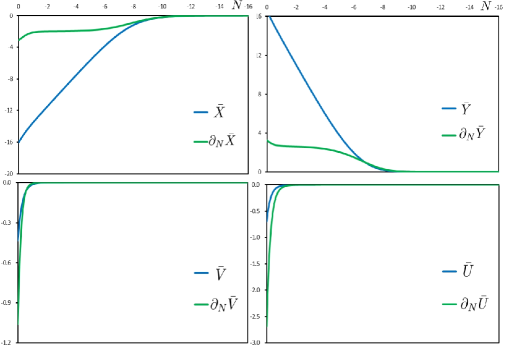
Figure 1: The evolution of the background scalars $\bar{X},\,\bar{Y},\,\bar{V},\,\bar{U}$ and their derivatives with respect to the $\boldsymbol{e}$-folding time $N$.

Applying the numerical results and the one-to-one relation between $\bar{Y}(N)$ and $f(N)$, the nonlocal distortion function $f(\bar{Y})$ is fixed as

$$f(\bar{Y})\simeq\boldsymbol{e}^{\,2.153\,(\bar{Y}-16.97)}.$$ (3.10)

This fitted function has the small deviation with the result in [27], as shown in FIG. 2, which may result from the small difference of the initial conditions.

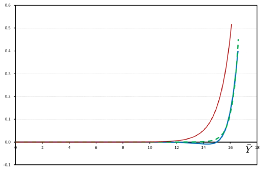
Figure 2: The curves of the full numerical determination of $f(\bar{Y})$ (the solid blue curve), the resulting exponential fit (3.10) (the dashed green curve) and the fitted function proposed by [27] (the crimson curve).

In order to test the self-consistency of our numerical results, we checked the EoS parameter $w_{de}$ of the effective dark energy component provided by the nonlocal modifications in DW-2019 model,

$$w_{de}=\frac{\bar{p}_{de}}{\bar{\rho}_{de}},$$ (3.11)

where $\bar{\rho}_{de}\equiv-\frac{1}{8\pi Ga^{2}}\Delta\bar{G}_{00}$ and $\bar{p}_{de}\equiv-\frac{1}{8\pi Ga^{2}}\Delta\bar{G}_{11}$. The result in FIG. 3 shows $w_{de}$ approaches to $-1$ very closely, consisting with the precondition (the $\Lambda$CDM background) well.

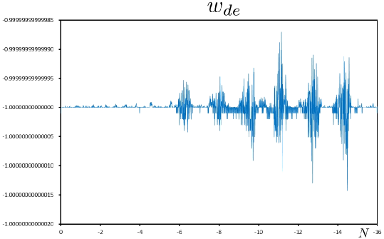
Figure 3: The numerical result of the EoS parameter $w_{de}$ under the $\Lambda$CDM background in the DW-2019 model.

3.2 The matter density perturbation in DW-2019 model

In the $\boldsymbol{e}$-folding time $N$, the growth equation for the matter density perturbation (2.37) can be transformed into

$$\partial^{2}_{N}\delta_{m}+(\xi+2)\,\partial_{N}\delta_{m}=G_{N}\cdot\frac{3}{2}\,\Omega_{m0}\,\frac{H^{2}_{0}}{H^{2}}\,\boldsymbol{e}^{-3N}\,\delta_{m}.$$ (3.12)

The initial conditions of $\delta_{m}$ deep into the matter dominated era are taken to consist with the pure CDM model [25]

$$\delta_{m}(N^{*}_{ini})=a^{*}_{ini},\indent\frac{\partial_{N}\delta_{m}(N^{*}_{ini})}{\delta_{m}(N^{*}_{ini})}=1,\indent(N^{*}_{ini}=\ln{a^{*}_{ini}})$$ (3.13)

where the initial scalar factor $a^{*}_{ini}$ is taken at redshift $z^{*}_{ini}=9$.

Based on the numerical results from reconstructing process, we solved Eq. (3.12) numerically. As shown in FIG. 6, the evolving curve of $\partial_{N}\delta_{m}$ has a peculiar null point at $z\simeq 0.39$ that leads to the discontinuity of $\delta_{m}$, which is different from the case of the DW model. In order to explain this puzzle, we focused on the difference between the DW model and the DW-2019 model. The nonlocal distortion function of the DW model is defined as the function of the scalar field $\bar{X}$ that sources from the Ricci scalar of the universe as shown in Eq.(2.2). For the DW-2019 model, the nonlocal distortion function is defined as the function of the new scalar field $\bar{Y}$ whose source is proportional to the square of the rate of change of $\bar{X}$ as shown in Eq.(2.3). The evolving curves of these two nonlocal distortion functions are illustrated in FIG. 4, which shows the amplitude of variation of $f(\bar{Y})$ of the DW-2019 model is greater than $f(\bar{X})$ of the DW model. Hence the form of nonlocal modification in the action of the DW-2019 model may provide a stronger nonlocal effect than that of the DW model. On the other hand, based on the numerical results as illustrated in FIG. 5, beyond the $\Lambda$CDM background, we find that the auxiliary scalar field $\bar{V}$ is negative and the term of $(1+\bar{U}+f(\bar{Y}))$ keeps positive, and $\bar{V}$ decreases faster than the increasing rate of $(1+\bar{U}+f(\bar{Y}))$, which makes $1+\bar{U}+f(\bar{Y})+6\bar{V}\rightarrow 0$ at $N\simeq-0.328$ ($z\simeq 0.39$) so that $G_{N}$ is divergent at this point. These numerical characteristics directly lead to the discontinuities of $\partial_{N}\delta_{m}$ and the growth rate $f\sigma_{8}$.

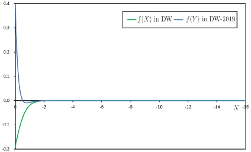
Figure 4: The comparison of the nonlocal distortion function in the DW model and the DW-2019 model via numerical methods.

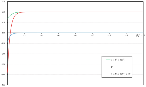
Figure 5: The numerical results of $(1+\bar{U}+f(\bar{Y}))$, $\bar{V}$ and $(1+\bar{U}+f(\bar{Y})+6\bar{V})$.

In brief, the nonlocal effect behaves as a cumulative effect. In the high-redshift range this cumulative effect is weak and the DW-2019 model can reduce to GR. After a long time with the accumulation and turning into the low-redshift range, the nonlocal effect is stronger enough to impact the matter perturbation.

The measurements of the growth rate $f\sigma_{8}$ at different redshift $z$ can be used to test the theories of dark energy and the modified gravities. $f$ represents the structural growth rate of universe and $\sigma_{8}$ is the amplitude of matter fluctuations in spheres of $8\,h^{-1}$ Mpc, defined by

$$f\equiv\partial_{N}(\ln\delta_{m}),\quad\sigma_{8}(N)\equiv\sigma^{0}_{8}\,\frac{\delta_{m}(N)}{\delta_{m}(0)}.$$ (3.14)

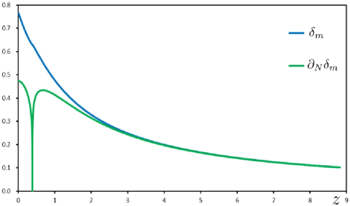
Figure 6: The matter perturbation $\delta_{m}$ and its derivative $\partial_{N}\delta_{m}$ at different redshift $z$ in the DW-2019 model under the $\Lambda$CDM background(3.5).

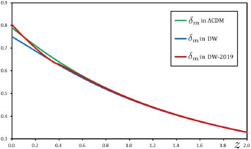
Figure 7: The comparison of the different matter perturbation $\delta_{m}(z)$ in the $\Lambda$CDM, DW model and DW-2019 model.

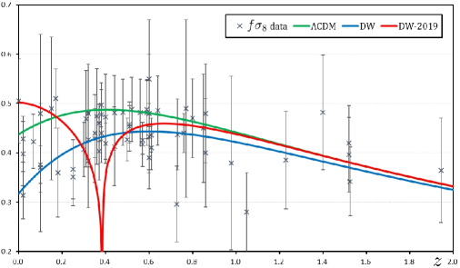
Figure 8: The predicted $f\sigma_{8}$ at different redshift $z$ provided by $\Lambda$CDM, DW and DW-2019 models under the background(3.5), and the $f\sigma_{8}$ data from RSD measurements that are shown in TABLE 1 and 2 in Appendix.

Using $N=-\ln(z+1)$, we plotted the numerical result of $f\sigma_{8}(z)$ under the DW-2019 model in FIG.8. As shown in FIG.8, our numerical result of $f\sigma_{8}(z)$ under the DW model is consistent with the result in [25]. The predicted values of $f\sigma_{8}(z)$ under the DW-2019 model can not provide a good fit with the low-redshift RSD measurements. Moreover, there is a distinct and unnatural plummet of the growth rate curve at $z\simeq 0.39$, which is caused by the above-mentioned discontinuity of the matter perturbation $\delta_{m}$ sourced by the strong nonlocal modification in the DW-2019 model. In another word, the DW-2019 model produces a strong nonlocal effect corresponding to the dark energy, which provides a more dramatic evolution of the matter perturbation $\delta_{m}$. In Sec. 4, based on the gravitational slip we will discuss it further. In addition, the clear difference of the predicted $f\sigma 8$ between these models appears in the low-redshift range, which illustrates that the low-redshift RSD measurement is an efficient tool to distinguish and test these models.

4 Gravitational Slip

Whereas GR predicts $\Psi=\Phi$ in the presence of nonrelativistic matter, the difference between the amplitudes of the Newtonian ($\Psi$) and longitudinal ($\Phi$) gravitational potentials, called gravitational slip [31, 32], usually can be understood as the effective anisotropic stress in modified gravity theories. The gravitational slip is a key variable in the characterization of the physical origin of the dark energy. For convenience, for the DW-2019 model we defined the gravitational slip as

$$\frac{\Psi-\Phi}{\Psi+\Phi}=\frac{2\bar{V}}{1+\bar{U}+f(\bar{Y})+6\bar{V}}.$$ (4.1)

Based on the zeroth-order part of the (00) component of field equations (2.9) and Eqs. (LABEL:solution_of_psi)(LABEL:solution_of_phi), $\Psi$ and $\Phi$ can be written into

$$\Psi=-\frac{3}{2}\,\frac{\mathcal{H}^{2}}{k^{2}}\,\delta_{m}\cdot C_{\Psi},$$ (4.2)

$$\Phi=-\frac{3}{2}\,\frac{\mathcal{H}^{2}}{k^{2}}\,\delta_{m}\cdot C_{\Phi},$$

where $C_{\Psi}$ and $C_{\Phi}$ are the modified factors sourced by the DW-2019 model, given by

$$C_{\Psi}=\frac{1+\bar{U}+f(\bar{Y})+8\bar{V}}{(1+\bar{U}+f(\bar{Y}))(1+\bar{U}+f(\bar{Y})+6\bar{V})}\cdot\bigg{\{}1+\bar{U}+f(\bar{Y})+\partial_{N}\bar{U}+f^{(1)}(\bar{Y})\partial_{N}\bar{Y}$$ (4.3)

$$\indent\indent\quad+\frac{1}{6}\big{[}\partial_{N}\bar{X}\partial_{N}\bar{U}+\partial_{N}\bar{Y}\partial_{N}\bar{V}+\bar{V}(\partial_{N}\bar{X})^{2}\big{]}\bigg{\}},$$

$$C_{\Phi}=\frac{1+\bar{U}+f(\bar{Y})+4\bar{V}}{(1+\bar{U}+f(\bar{Y}))(1+\bar{U}+f(\bar{Y})+6\bar{V})}\cdot\bigg{\{}1+\bar{U}+f(\bar{Y})+\partial_{N}\bar{U}+f^{(1)}(\bar{Y})\partial_{N}\bar{Y}$$ (4.4)

$$\indent\indent\quad+\frac{1}{6}\big{[}\partial_{N}\bar{X}\partial_{N}\bar{U}+\partial_{N}\bar{Y}\partial_{N}\bar{V}+\bar{V}(\partial_{N}\bar{X})^{2}\big{]}\bigg{\}}.$$

When $C_{\Psi}$ and $C_{\Psi}$ both degenerate to $1$, these two potentials will reduce to those of GR.

With the basis of the reconstructed numerical results, we plotted the evolving curves of $C_{\Psi}$ and $C_{\Phi}$ in FIG. 9, which illustrates that $C_{\Psi}$ and $C_{\Phi}$ both diverges at $z\simeq 0.39$ where $1+\bar{U}+f(\bar{Y})+6\bar{V}=0$. On the contrary, $(C_{\Psi}+C_{\Phi})/2$ evolves smoothly without the divergency, which shows the sum of $\Psi$ and $\Phi$ always behaves regularly. This explains that in the sub-horizon limit ($k\gg\mathcal{H}$) the results from the linear perturbation theory is still reliable and self-consistent as a whole.

On the other hand, the gravitational slip represents the anisotropic effect in the modified gravities, so the strong gravitational slip may influence the evolution of the matter perturbation $\delta_{m}$. FIG. 10 shows the amplitude of the gravitational slip of the DW-2019 model is stronger than that of the DW model, which shows the DW-2019 model may provide more dark energy parts to impact the evolution of the matter perturbation $\delta_{m}$. And that is one possible cause of leading to the discontinuity of the growth rate $f\sigma_{8}$.

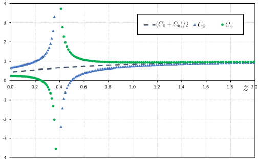
Figure 9: The evolving curves of $C_{\Psi}$, $C_{\phi}$ and $(C_{\Psi}+C_{\Phi})/2$.

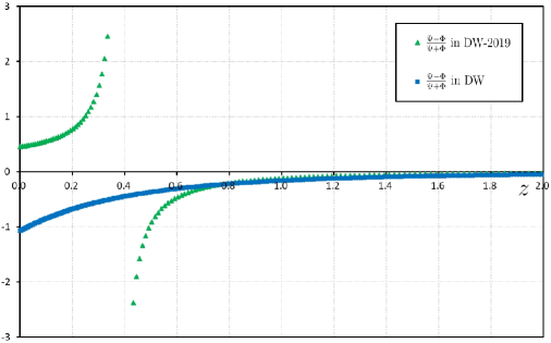
Figure 10: The evolution of the gravitational slip respectively in the DW and DW-2019 model.

5 The Free Screening Mechanism

The time variation of the effective Newtonian gravitational constant is another important criterion to test modified gravities [26, 33]. In the DW-2019 model, the effective Newtonian gravitational constant $G_{eff}=\big{[}1+\bar{U}+f(\bar{Y})\big{]}^{-1}\,G$ and its time variation is

$$\frac{\dot{G}_{eff}}{G_{eff}}=-\frac{\partial_{N}\bar{U}+f^{(1)}(\bar{Y})\,\partial_{N}\bar{Y}}{1+\bar{U}+f(\bar{Y})}\,H.$$ (5.1)

Using the numerical results, the time variation of Newtonian gravitational constant in DW-2019 model is given by

$$\bigg{|}\frac{\dot{G}_{eff}}{G_{eff}}\bigg{|}\simeq 0.717H_{0}\sim\mathcal{O}(H_{0}).$$ (5.2)

On the other hand, Lunar Laser Ranging observation provides a strict limit on the time variation of Newtonian gravitational constant [26, 34]

$$\frac{\dot{G}}{G} =(7.1\pm 7.6)\times 10^{-14}\,yr^{-1}$$ (5.3)

$$=(0.99\pm 1.06)\cdot(\frac{0.7}{h_{0}})\times 10^{-3}\cdot H_{0}$$

$$\sim\mathcal{O}(10^{-3}\,H_{0}).$$

Hence DW-2019 model seems to be ruled out by Lunar Laser Ranging observation. However, there may exist a natural screening mechanism provided by the inverse scalar d’Alembertian. There is no reason to apply the FLRW solution in the strongly bound matter regime because the uneven matter distribution must curve spacetime. In order to solve this problem, connecting the cosmological regime with the strongly bound matter regime, one applied the McVittie metric [26] as the background metric,

$$ds^{2}=-\big{[}1-\Upsilon(r)-r^{2}H^{2}\big{]}dt^{2}-\frac{2rH}{\sqrt{1-\Upsilon(r)}}drdt+\frac{1}{1-\Upsilon(r)}dr^{2}+r^{2}d\Omega^{2},$$ (5.4)

where $\Upsilon(r)=r_{s}/r$. $r_{s}$ is the Schwarzschild radius of the central object of mass M. The McVittie metric reduces to the FRW solution as $M\rightarrow 0$, and to the Schwarzschild solution as $H\rightarrow 0$. In order to test the modified gravities by the Lunar Laser Ranging, we should consider the circumstance of the Earth-Moon scales. For an actual observer , the central object can be simply regarded as Earth whose Schwarzschild radius is far less than its radius, which states $\Upsilon\ll 1$. In fact, this condition is always reasonable as long as the central object is not a black hole. In addition, for the different cases of gravitationally bound systems, the general McVittie metric was presented by generalizing the form of $\Upsilon(r)$ [26].

Based on the McVittie metric, one can obtain the Ricci scalar

$$R(t,r)=12H^{2}+\frac{6\dot{H}}{\sqrt{1-\Upsilon}}+\frac{2}{r^{2}}\,\Upsilon+\frac{4}{r}\,\partial_{r}\Upsilon+\partial^{2}_{r}\Upsilon$$ (5.5)

and the scalar equations $S(t,r)=\Box J(t,r)$ can be expanded as

$$S(t,r)= -\frac{1}{1-\Upsilon}\,\partial^{2}_{t}J-\frac{3H}{\sqrt{1-\Upsilon}}\,\partial_{t}J-\frac{1}{2}\frac{r\,\partial_{r}\Upsilon H}{(1-\Upsilon)^{3/2}}\,\partial_{t}J$$ (5.6)

$$+(1-\Upsilon-r^{2}H^{2})\,\partial^{2}_{r}J+\frac{2}{r}\,[1-\Upsilon-2r^{2}H^{2}-\frac{1}{2}r\,\partial_{r}\Upsilon]\,\partial_{r}J$$

$$-\frac{r\dot{H}}{\sqrt{1-\Upsilon}}\partial_{r}J-\frac{rH}{\sqrt{1-\Upsilon}}(\partial_{t}\partial_{r}J+\partial_{r}\partial_{t}J),$$

where $S$ represents the source of the nonlocal modification $J$ and $J=X,\,Y,\,V,\,U$. Applying the above condition of $\Upsilon\ll 1$, the Ricci scalar and the scalar equations can be simplified into

$$R(t,r)=12H^{2}+6\dot{H}+\frac{2}{r^{2}}\,\Upsilon+\frac{4}{r}\,\partial_{r}\Upsilon+\partial^{2}_{r}\Upsilon,$$ (5.7)

$$S(t,r) =-\frac{1}{a^{3}}\,\partial_{t}(\,a^{3}\,\partial_{t}J\,)+\frac{1}{r^{2}}\,\partial_{r}(\,r^{2}\,\partial_{r}J\,)-r^{2}\,H^{2}\,\big{[}\,\partial^{2}_{r}J+\frac{1}{r}\,(4-\epsilon)\,\partial_{r}J\,\big{]}$$ (5.8)

$$\indent\indent-r\,H\,(\,\partial_{t}\partial_{r}J+\partial_{r}\partial_{t}J\,),$$

where $\epsilon\equiv-\frac{\dot{H}}{H^{2}}$ that is the slowly-varying Hubble parameter.

For the gravitationally bound systems with Earth-Moon scales, we have the constraint of $rH\ll 1$ and the expression of $S(t,r)$ can be further simplified into

$$S(t,r)=-\frac{1}{a^{3}}\partial_{t}(a^{3}\partial_{t}J)+\frac{1}{r^{2}}\partial_{r}(r^{2}\partial_{r}J).$$ (5.9)

For the scalar field $X$ ($J=X$), the source is the Ricci scalar ($S=R$). Because the source $R$ has the superimposed form of $R(t,r)=R_{cosmo}(t)+R_{static}(r)$ as shown in Eq.(5.7), $X$ can be chosen as a simple superimposed form $X(t,r)=X_{cosmo}(t)+X_{static}(r)$. It is worth mentioning that $R_{cosmo}(t)$ is provided by the expansion of the unverse which belongs to the large-scale effect and $R_{static}(r)$ is provided by the inhomogeneity of matter distribution which belongs to the small-scale effect.

For the case of the scalar field $Y$ whose source is $S=g^{\mu\nu}\partial_{\mu}X\partial_{\nu}X$, the scalar equation of $Y$ can be expanded as

$$-(\partial_{t}X_{cosmo})^{2}+(\partial_{r}X_{static})^{2}\simeq-\frac{1}{a^{3}}\partial_{t}(a^{3}\partial_{t}Y)+\frac{1}{r^{2}}\partial_{r}(r^{2}\partial_{r}Y).$$ (5.10)

Then $Y(t,r)$ has the superimposed form of $Y_{cosmo}(t)+Y_{static}(r)$ as well. Therefore, for the scalar fields $X$ and $Y$, the contributions from the large-scale effect and the small-scale effect are linearly superimposed.

However, for the scalar fields $V(t,r)$ and $U(t,r)$, things are going to change. Assuming that the nonlocal distortion function $f(Y)$ (3.10) is still applicative in the small-scale range, the source function of $V$ is

$$R\,f^{(1)}(Y) =[R_{cosmo}(t)+R_{static}(r)]\cdot f^{(1)}(Y_{cosmo}(t)+Y_{static}(r))$$ (5.11)

$$\propto\,R_{cosmo}(t)\cdot f^{(1)}(Y_{cosmo}(t))\cdot f^{(1)}(Y_{static}(r))$$

$$\indent\quad+R_{static}(r)\cdot f^{(1)}(Y_{cosmo}(t))\cdot f^{(1)}(Y_{static}(r)).$$

Obviously the scalar field $V$ can be not written into the superimposed form like $X$ and $Y$, because its source function has the cross terms of time and space. From Eq.(2.5), we can estimate that $U$ has an intricate form of $(t,r)$ including the cross terms of $(t,r)$ as well.

For the sake of illustration, considering the small-scale effect, we obtained the generalization of the time variation of Newtonian’s constant qualitatively, given by

$$\frac{\dot{G}_{eff}}{G_{eff}}\sim-\frac{\partial_{N}U(t,r)+2.153\,\boldsymbol{e}^{2.153\,(Y_{cosmo}+Y_{static}-16.97)}\,\partial_{N}Y_{cosmo}}{1+U(t,r)+\boldsymbol{e}^{2.153\,(Y_{cosmo}+Y_{static}-16.97)}}\cdot H.$$ (5.12)

Unlike the linear superposition of the large-scale effect and the small-scale effect in $X$ and $Y$, these two kinds of effects appear as the nonlinear recombination in the scalar fields $U(t,r)$ and $V(t,r)$. Therefore, there is the possibility that the small-scale effect is magnified in $V$ or $U$ to produce a free screening mechanism. With the help of the general McVittie metric, the deeper research can be studied in the future.

6 Conclusions

In this work, we derive the first-order field equations of the DW-2019 model by the cosmological perturbation theory. In order to study the growth rate beyond the $\Lambda$CDM background, firstly we apply the reconstructing technique to obtain the evolution of the background fields in the DW-2019 model, and the nonlocal distortion function $f(Y)$ is fitted as $f(Y)\simeq\boldsymbol{e}^{2.153(Y-16.97)}$. For the purpose of testing the reasonability of our numerical method, we calculate the growth rate $f\sigma_{8}$ predicted by the DW model that has a good consistency with the result in [25], which shows our numerical method is feasible. In the DW-2019 model, based on the numerical results from the reconstructing process, the predicted growth rate $f\sigma_{8}(z)$ is obtained, which deviates from $f\sigma_{8}$ data of the RSD measurements to some extent, as shown in FIG.8. Even so, the DW-2019 model still can not be ruled out by the RSD measurements and its reliability should be tested further by the low-redshift RSD measurements. Moreover, for the DW-2019 model, the evolving curve of the growth rate $f\sigma_{8}$ has an unnatural plummet at $z\simeq 0.39$. Based on the numerical results, we find the direct reason is $1+\bar{U}+f(\bar{Y})+6\bar{V}=0$ at $z\simeq 0.39$, which leads to the divergency of $G_{N}$ in the second-order differential equation of $\delta_{m}$. From the perspective of theoretical analysis, the possible cause is that the DW-2019 model produces a strong nonlocal effect which behaves as the strong anisotropic stress corresponding to the dark energy in the low-redshift range to impact the evolution of the matter perturbation. At last, by the qualitative analysis of the DW-2019 model, we pointed out that the spacial dependence of the nonlocal modification in the small-scale range may provide a free screening mechanism, in the meantime, perhaps it will produce the correction for the matter perturbation in the low-redshift range as well.

Appendix

Table 1: The $f\,\sigma_{8}$ data provided by the RSD measurements from various sources[35].

Survey	$z$	$f\,\sigma_{8}$	Ref.	Year
SDSS-LRG	0.35	0.44 $\pm$ 0.05	[36]	2006
VVDS	0.77	0.49 $\pm$ 0.18	[36]	2009
2dFGRS	0.17	0.51 $\pm$ 0.06	[36]	2009
2MRS	0.02	0.314 $\pm$ 0.048	[37],[38]	2010
SnIa-IRAS	0.02	0.398 $\pm$ 0.065	[38],[39]	2011
SDSS-LRG-200	0.25	0.3512 $\pm$ 0.00583	[40]	2011
SDSS-LRG-200	0.37	0.4602 $\pm$ 0.0378	[40]	2011
SDSS-LRG-60	0.25	0.3665 $\pm$ 0.0601	[40]	2011
SDSS-LRG-60	0.37	0.4031 $\pm$ 0.0586	[40]	2011
WiggleZ	0.44	0.413 $\pm$ 0.08	[41]	2012
WiggleZ	0.6	0.39 $\pm$ 0.063	[41]	2012
WiggleZ	0.73	0.437 $\pm$ 0.072	[41]	2012
6dFGS	0.067	0.423 $\pm$ 0.055	[42]	2012
SDSS-BOSS	0.3	0.407 $\pm$ 0.055	[43]	2012
SDSS-BOSS	0.4	0.419 $\pm$ 0.041	[43]	2012
SDSS-BOSS	0.5	0.427 $\pm$ 0.043	[43]	2012
SDSS-BOSS	0.6	0.433 $\pm$ 0.067	[43]	2012
Vipers	0.8	0.47 $\pm$ 0.08	[44]	2013
SDSS-DR7-LRG	0.35	0.429 $\pm$ 0.089	[45]	2013
GAMA	0.18	0.36 $\pm$ 0.09	[46]	2013
GAMA	0.38	0.44 $\pm$ 0.06	[46]	2013
BOSS-LOWZ	0.32	0.384 $\pm$ 0.095	[47]	2013
SDSS DR10/11	0.32	0.48 $\pm$ 0.1	[47]	2013
SDSS DR10/11	0.57	0.417 $\pm$ 0.045	[47]	2013
SDSS-MGS	0.15	0.49 $\pm$ 0.145	[48]	2015
SDSS-veloc	0.1	0.37 $\pm$ 0.13	[49]	2015
FastSound	1.4	0.482 $\pm$ 0.116	[50]	2015
SDSS-CMASS	0.59	0.488 $\pm$ 0.06	[51]	2016
BOSS DR12	0.38	0.497 $\pm$ 0.045	[52]	2016
BOSS DR12	0.51	0.458 $\pm$ 0.038	[52]	2016
BOSS DR12	0.61	0.436 $\pm$ 0.034	[52]	2016

Table 2: The $f\,\sigma_{8}$ data following the above table

Survey	$z$	$f\,\sigma_{8}$	Ref.	Year
BOSS DR12	0.38	0.477 $\pm$ 0.051	[53]	2016
BOSS DR12	0.51	0.453 $\pm$ 0.05	[53]	2016
BOSS DR12	0.61	0.41 $\pm$ 0.044	[53]	2016
Vipers v7	0.76	0.44 $\pm$ 0.04	[54]	2016
Vipers v7	1.05	0.28 $\pm$ 0.08	[54]	2016
BOSS LOWZ	0.32	0.427 $\pm$ 0.056	[55]	2016
BOSS CMASS	0.57	0.426 $\pm$ 0.029	[55]	2016
Vipers	0.727	0.296 $\pm$ 0.0765	[56]	2016
6dFGS+SnIa	0.02	0.428 $\pm$ 0.0465	[57]	2016
Vipers	0.6	0.48 $\pm$ 0.12	[58]	2016
Vipers	0.86	0.48 $\pm$ 0.1	[58]	2016
Vipers PDR-2	0.6	0.55 $\pm$ 0.12	[59]	2016
Vipers PDR-2	0.86	0.4 $\pm$ 0.11	[59]	2016
SDSS DR13	0.1	0.48 $\pm$ 0.16	[60]	2016
2MTF	0.001	0.505 $\pm$ 0.085	[61]	2017
Vipers PDR-2	0.85	0.45 $\pm$ 0.11	[62]	2017
BOSS DR12	0.31	0.469 $\pm$ 0.098	[63]	2017
BOSS DR12	0.36	0.474 $\pm$ 0.097	[63]	2017
BOSS DR12	0.4	0.473 $\pm$ 0.086	[63]	2017
BOSS DR12	0.44	0.481 $\pm$ 0.076	[63]	2017
BOSS DR12	0.48	0.482 $\pm$ 0.067	[63]	2017
BOSS DR12	0.52	0.488 $\pm$ 0.065	[63]	2017
BOSS DR12	0.56	0.482 $\pm$ 0.067	[63]	2017
BOSS DR12	0.59	0.481 $\pm$ 0.066	[63]	2017
BOSS DR12	0.64	0.486 $\pm$ 0.07	[63]	2017
SDSS DR7	0.1	0.376 $\pm$ 0.038	[64]	2017
SDSS-IV	1.52	0.42 $\pm$ 0.076	[65]	2018
SDSS-IV	1.52	0.396 $\pm$ 0.076	[66]	2018
SDSS-IV	0.978	0.379 $\pm$ 0.176	[67]	2018
SDSS-IV	1.23	0.385 $\pm$ 0.099	[67]	2018
SDSS-IV	1.526	0.342 $\pm$ 0.07	[67]	2018
SDSS-IV	1.944	0.364 $\pm$ 0.106	[67]	2018

References

- [1] Adam G Riess, et al. Observational evidence from supernovae for an accelerating universe and a cosmological constant, The Astronomical Journal, 116 (1998) 1009.
- [2] Saul Perlmutter, et al. Measurements of and from 42 high-redshift supernovae, The Astrophysical Journal, 517 (1999) 565.
- [3] Clifford M Will. The confrontation between general relativity and experiment, Living reviews in relativity, 9 (2006) 3.
- [4] Bharat Ratra and Philip JE Peebles. Cosmological consequences of a rolling homogeneous scalar field, Phys. Rev. D, 37 (1988) 3406.
- [5] Christof Wetterich. Cosmology and the fate of dilatation symmetry, Nuclear Physics B, 302 (1988) 668–696.
- [6] NC Tsamis and RP Woodard. Nonperturbative models for the quantum gravitational back-reaction on inflation, Annals of Physics, 267 (1998) 145–192.
- [7] S Capozziello, S Nojiri, and SD Odintsov. Dark energy: the equation of state description versus scalar-tensor or modified gravity, Physics Letters B, 634 (2006) 93–100.
- [8] Shin’Ichi Nojiri and Sergei D Odintsov. Introduction to modified gravity and gravitational alternative for dark energy, International Journal of Geometric Methods in Modern Physics, 4 (2007) 115–145.
- [9] Richard Woodard. Avoiding dark energy with modifications of gravity, Springer (2007).
- [10] Tarun Deep Saini, et al. Reconstructing the cosmic equation of state from supernova distances, Phys. Rev. Lett., 85 (2000) 1162.
- [11] Gilles Esposito-Farèse and David Polarski. Scalar-tensor gravity in an accelerating universe, Phys. Rev. D, 63 (2001) 063504.
- [12] Christof Wetterich. Effective nonlocal Euclidean gravity, General Relativity and Gravitation, 30 (1998) 159–172.
- [13] RP Woodard. Nonlocal models of cosmic acceleration, Foundations of Physics, 44 (2014) 213–233.
- [14] Richard Woodard. The Case for Nonlocal Modifications of Gravity, Universe, 4 (2018) 88.
- [15] Valeri Vardanyan, Yashar Akrami, Luca Amendola and Alessandra Silvestri. On nonlocally interacting metrics, and a simple proposal for cosmic acceleration, Journal of Cosmology and Astroparticle Physics, 2018 (2018) 048.
- [16] Valeri Vardanyan, Yashar Akrami, Luca Amendola and Alessandra Silvestri. On nonlocally interacting metrics, and a simple proposal for cosmic acceleration, Journal of Cosmology and Astroparticle Physics, 2018 (2018) 048–048.
- [17] Michele Maggiore and Michele Mancarella. Nonlocal gravity and dark energy, Phys. Rev. D, 90 (2014) 023005.
- [18] Alessandro Codello and Rajeev Kumar Jain. A unified universe, The European Physical Journal C, 78 (2018) 357.
- [19] Henrik Nersisyan, Yashar Akrami, Luca Amendola, Tomi S.Koivisto, and Javier Rubio. Dynamical analysis of cosmology: Impact of initial conditions and constraints from supernovae, Phys. Rev. D, 94 (2016) 043531.
- [20] Shuxun Tian, Scalar-tensor nonlocal gravity, Phys. Rev. D, 98 (2018) 084040.
- [21] Henrik Nersisyan, Yashar Akrami, Luca Amendola, Tomi S. Koivisto, Javier Rubio and Adam R.Solomon. Instabilities in tensorial nonlocal gravity, Phys. Rev. D, 95 (2017) 043539.
- [22] Salvatore Capozziello, Emilio Elizalde, Shin’ichi Nojiri and Sergei D Odintsov. Accelerating cosmologies from non-local higher-derivative gravity, Physics Letters B, 671 (2009) 193–198.
- [23] S. Deser, and R. P. Woodard. Nonlocal Cosmology, Phys. Rev. Lett., 99 (2007) 111301.
- [24] C Deffayet and RP Woodard. Reconstructing the distortion function for nonlocal cosmology, Journal of Cosmology and Astroparticle Physics, 2009 (2009) 023.
- [25] Henrik Nersisyan, Adrian Fernandez Cid and Luca Amendola. Structure formation in the Deser-Woodard nonlocal gravity model: a reappraisal, Journal of Cosmology and Astroparticle Physics, 2017 (2017) 046.
- [26] Enis Belgacem, Andreas Finke, Antonia Frassinoa and Michele Maggiore. Testing nonlocal gravity with lunar laser ranging, Journal of Cosmology and Astroparticle Physics, 2019 (2019) 035.
- [27] S Deser and RP Woodard. Nonlocal cosmology II. Cosmic acceleration without fine tuning or dark energy, Journal of Cosmology and Astroparticle Physics, 2019 (2019) 034.
- [28] Scott Dodelson and Sohyun Park. Nonlocal gravity and structure in the Universe, Phys. Rev. D, 90 (2014) 043535.
- [29] Daniel Baumann. Cosmology, University of Cambridge, (2015).
- [30] N Aghanim, et al. Planck 2018 results. VI. Cosmological parameters, arXiv:1807.06209.
- [31] Scott F. Daniel, Robert R. Caldwell, Asantha Cooray and Alessandro Melchiorri. Large scale structure as a probe of gravitational slip, Phys. Rev. D, 77 (2008) 103513.
- [32] Luca Amendola, Simone Fogli, Alejandro Guarnizo, Martin Kunz and Adrian Vollmer. Model-independent constraints on the cosmological anisotropic stress, Phys. Rev. D, 89 (2014) 063538.
- [33] S. X. Tian and Zong-Hong Zhu. Newtonian approximation and possible time-varying in nonlocal gravities, Phys. Rev. D, 99 (2019) 064044.
- [34] Franz Hofmann and Jürgen Müller. Relativistic tests with lunar laser ranging, Classical and Quantum Gravity, 35 (2018) 035015.
- [35] Lavrentios Kazantzidis and Leandros Perivolaropoulos. Evolution of the tension with the determination and implications for modified gravity theories, Phys. Rev. D, 97 (2018) 103503.
- [36] Yong-Seon Song and Will J Percival. Reconstructing the history of structure formation using redshift distortions, Journal of Cosmology and Astroparticle Physics, 2009 (2009) 004.
- [37] Marc Davis, Adi Nusser, Karen L Masters, Christopher Springob, John P Huchra and Gerard Lemson. Local gravity versus local velocity: solutions for and non-linear bias, Monthly Notices of the Royal Astronomical Society, 413 (2011) 2906–2922.
- [38] Michael J Hudson and Stephen J Turnbull. The growth rate of cosmic structure from peculiar velocities at low and high redshifts, The Astrophysical Journal Letters, 751 (2012) L30.
- [39] Stephen J Turnbull, Michael J Hudson, Hume A Feldman, Malcolm Hicken, Robert P Kirshner and Richard Watkins. Cosmic flows in the nearby universe from Type Ia Supernovae, Monthly Notices of the Royal Astronomical Society, 420 (2012) 447–454.
- [40] Lado Samushia, Will J Percival and Alvise Raccanelli. Interpreting large-scale redshift-space distortion measurements, Monthly Notices of the Royal Astronomical Society, 420 (2012) 2102–2119.
- [41] Chris Blake, et al. The WiggleZ Dark Energy Survey: Joint measurements of the expansion and growth history at , Monthly Notices of the Royal Astronomical Society, 425 (2012) 405–414.
- [42] Florian Beutler, et al. The 6dF Galaxy Survey: measurements of the growth rate and 8, Monthly Notices of the Royal Astronomical Society, 423 (2012) 3430–3444.
- [43] Rita Tojeiro, et al. The clustering of galaxies in the SDSS-III Baryon Oscillation Spectroscopic Survey: measuring structure growth using passive galaxies, Monthly Notices of the Royal Astronomical Society, 424 (2012) 2339–2344.
- [44] S De La Torre, et al. The VIMOS Public Extragalactic Redshift Survey (VIPERS)-Galaxy clustering and redshift-space distortions at in the first data release, Astronomy & Astrophysics, 557 (2013) A54.
- [45] Chia-Hsun Chuang and Yun Wang. Modelling the anisotropic two-point galaxy correlation function on small scales and single-probe measurements of H (z), DA (z) and f (z) 8 (z) from the Sloan Digital Sky Survey DR7 luminous red galaxies, Monthly Notices of the Royal Astronomical Society, 435 (2013) 255–262.
- [46] Chris Blake, et al. Galaxy And Mass Assembly (GAMA): improved cosmic growth measurements using multiple tracers of large-scale structure, Monthly Notices of the Royal Astronomical Society, 436 (2013) 3089–3105.
- [47] Ariel G Sanchez, et al. The clustering of galaxies in the SDSS-III Baryon Oscillation Spectroscopic Survey: cosmological implications of the full shape of the clustering wedges in the data release 10 and 11 galaxy samples, Monthly Notices of the Royal Astronomical Society, 440 (2014) 2692–2713.
- [48] Cullan Howlett, Ashley J Ross, Lado Samushia, Will J Percival and Marc Manera. The clustering of the SDSS main galaxy sample–II. Mock galaxy catalogues and a measurement of the growth of structure from redshift space distortions at , Monthly Notices of the Royal Astronomical Society, 449 (2015) 848–866.
- [49] Martin Feix, Adi Nusser and Enzo Branchini. Growth Rate of Cosmological Perturbations at from a New Observational Test, Phys. Rev. Lett., 115 (2015) 011301.
- [50] Teppei Okumura, et al. The Subaru FMOS galaxy redshift survey (FastSound). IV. New constraint on gravity theory from redshift space distortions at z 1.4, Publications of the Astronomical Society of Japan, 68 (2016) 38.
- [51] Chia-Hsun Chuang, et al. The clustering of galaxies in the SDSS-III Baryon Oscillation Spectroscopic Survey: single-probe measurements from CMASS anisotropic galaxy clustering, Monthly Notices of the Royal Astronomical Society, 461 (2016) 3781–3793.
- [52] Shadab Alam, et al. The clustering of galaxies in the completed SDSS-III Baryon Oscillation Spectroscopic Survey: cosmological analysis of the DR12 galaxy sample, Monthly Notices of the Royal Astronomical Society, 470 (2017) 2617–2652.
- [53] Florian Beutler, et al. The clustering of galaxies in the completed SDSS-III Baryon Oscillation Spectroscopic Survey: anisotropic galaxy clustering in Fourier space, Monthly Notices of the Royal Astronomical Society, 466 (2016) 2242–2260.
- [54] Michael J Wilson. Geometric and growth rate tests of General Relativity with recovered linear cosmological perturbations, arXiv:1610.08362.
- [55] Héctor Gil-Marín, et al. The clustering of galaxies in the SDSS-III Baryon Oscillation Spectroscopic Survey: RSD measurement from the power spectrum and bispectrum of the DR12 BOSS galaxies, Monthly Notices of the Royal Astronomical Society, 465 (2016) stw2679.
- [56] AJ Hawken,et al. The VIMOS Public Extragalactic Redshift Survey-Measuring the growth rate of structure around cosmic voids, Astronomy & Astrophysics, 607 (2017) A54.
- [57] Dragan Huterer, Daniel L Shafer, Daniel M Scolnic and Fabian Schmidt. Testing CDM at the lowest redshifts with SN Ia and galaxy velocities, Journal of Cosmology and Astroparticle Physics, 2017 (2017) 015.
- [58] S de La Torre, et al. The VIMOS Public Extragalactic Redshift Survey (VIPERS)-Gravity test from the combination of redshift-space distortions and galaxy-galaxy lensing at , Astronomy & Astrophysics, 608 (2017) A44.
- [59] A Pezzotta, et al. The VIMOS Public Extragalactic Redshift Survey (VIPERS)-The growth of structure at from redshift-space distortions in the clustering of the PDR-2 final sample, Astronomy & Astrophysics, 604 (2017) A33.
- [60] Martin Feix, Enzo Branchini and Adi Nusser. Speed from light: growth rate and bulk flow at from improved SDSS DR13 photometry, Monthly Notices of the Royal Astronomical Society, 468 (2017) 1420–1425.
- [61] Cullan Howlett, et al. 2MTF–VI. Measuring the velocity power spectrum, Monthly Notices of the Royal Astronomical Society, 471 (2017) 3135–3151.
- [62] FG Mohammad, et al. The VIMOS Public Extragalactic Redshift Survey (VIPERS)-An unbiased estimate of the growth rate of structure at using the clustering of luminous blue galaxies, Astronomy & Astrophysics, 610 (2018) A59.
- [63] Yuting Wang, et al. The clustering of galaxies in the completed SDSS-III Baryon Oscillation Spectroscopic Survey: a tomographic analysis of structure growth and expansion rate from anisotropic galaxy clustering, Monthly Notices of the Royal Astronomical Society, 481 (2018) 3160–3166.
- [64] Feng Shi, et al. Mapping the Real Space Distributions of Galaxies in SDSS DR7. II. Measuring the Growth Rate, Clustering Amplitude of Matter, and Biases of Galaxies at Redshift , The Astrophysical Journal, 861 (2018) 137.
- [65] Héctor Gil-Marín, et al. The clustering of the SDSS-IV extended Baryon Oscillation Spectroscopic Survey DR14 quasar sample: structure growth rate measurement from the anisotropic quasar power spectrum in the redshift range , Monthly Notices of the Royal Astronomical Society, 477 (2018) 1604–1638.
- [66] Jiamin Hou, et al. The clustering of the SDSS-IV extended Baryon Oscillation Spectroscopic Survey DR14 quasar sample: anisotropic clustering analysis in configuration space, Monthly Notices of the Royal Astronomical Society, 480 (2018) 2521–2534.
- [67] Gong-Bo Zhao, et al. The clustering of the SDSS-IV extended Baryon Oscillation Spectroscopic Survey DR14 quasar sample: a tomographic measurement of cosmic structure growth and expansion rate based on optimal redshift weights, Monthly Notices of the Royal Astronomical Society, 482 (2018) 3497–3513.