Quantum master equations for a system interacting with quantum gas in the low density limit and for the semiclassical collision model

Abstract

A quantum system interacting with a dilute gas experiences irreversible dynamics. The corresponding master equation can be derived within two different approaches: The fully quantum description in the low-density limit and the semiclassical collision model, where the motion of gas particles is classical whereas their internal degrees of freedom are quantum. The two approaches have been extensively studied in the literature, but their predictions have not been compared. This is mainly due to the fact that the low-density limit is extensively studied for mathematical physics purposes, whereas the collision models have been essentially developed for quantum information tasks such as a tractable description of the open quantum dynamics. Here we develop and for the first time compare both approaches for a spin system interacting with a gas of spin particles. Using some approximations, we explicitly find the corresponding master equations including the Lamb shifts and the dissipators. The low density limit in the Born approximation for fast particles is shown to be equivalent to the semiclassical collision model in the stroboscopic approximation. We reveal that both approaches give exactly the same master equation if the gas temperature is high enough. This allows to interchangeably use complicated calculations in the low density limit and rather simple calculations in the collision model.

I Introduction

Any realistic quantum system is open because of unavoidable coupling to its environment. The theory of open quantum systems studies the effect of the surrounding environment on the system dynamics breuer-2002 . The environment can be represented as a large reservoir either in thermodynamic equilibrium schoeller-2018 or in a non-equilibrium state. The system-reservoir interaction entangles the system with the environmental degrees of freedom, which typically leads to the irreversible system decoherence. Such a decoherence significantly affects quantum transport cui-2006 ; talarico-2019 , molecular excitation dynamics and relaxation valkunas-2013 , and performance of quantum sensors degen-2017 . It is the decoherence that complicates the protocols of quantum information transmission wilde-2017 and processing nielsen-2000 ; filippov-2019 . This circumstance makes the study of decoherence an important field of research for the development of quantum technologies glaser-2015 .

The state of a quantum system is represented by the density operator $\varrho(t)$ that is a Hermitian positive-semidefinite unit-trace operator acting in the system Hilbert space ${\cal H}$. Let ${\cal T}({\cal H})$ be the space of trace class operators acting in ${\cal H}$. The open dynamics is usually described by the time-convolutionless master equation $\frac{d}{dt}\varrho(t)={\cal L}_{t}[\varrho(t)]$, which is obtained by averaging over the environmental degrees of freedom in the joint evolution of the system and the reservoir. The generator ${\cal L}_{t}:{\cal T}({\cal H})\mapsto{\cal T}({\cal H})$ is time-dependent in general, which may lead to non-Markovian effects rivas-2014 ; breuer-2016 ; de-vega-2017 ; benatti-2017 ; fc-2018 ; li-2018 ; luchnikov-2019 . There are physical situations, however, where the generator is time-independent within the characteristic timescale of system evolution. Microscopic derivations of the master equation

$$\frac{d}{dt}\varrho(t)={\cal L}[\varrho(t)]$$ (1)

can be obtained in the weak coupling limit van-hove-1954 ; davies-1974 ; spohn-1978 ; accardi-1990 , the singular coupling limit palmer-1977 ; gorini-1978 , the stochastic limit accardi-book ; pechen-2002 , the low density limit for gas environment dumcke-1985 ; accardi-1991 ; accardi-1992 ; rudnicki-1992 ; apv-2002 ; accardi-2003 ; pechen-2004 ; pechen-jmp-2006 , the stroboscopic limit in the collision model rau-1963 ; giovannetti-2012 ; lorenzo-2017 ; luchnikov-2017 , and the monitoring approach to derivation of linear Boltzmann equation hornberger-2007 ; hornberger-2008 ; vacchini-2009 ; smirne-2010 . In all these approximations, the particular form of ${\cal L}$ is expressed through the system-environment interaction Hamiltonian and the reservoir equilibrium state. The solution of the master equation (1) is given by the quantum dynamical semigroup $e^{{\cal L}t}$, whose complete positivity makes the generator ${\cal L}$ take the Gorini-Kossakowski-Sudarshan-Lindblad (GKSL) form gks-1976 ; lindblad-1976 :

$${\cal L}[\varrho]=-\frac{i}{\hbar}[H,\varrho]+\sum_{k}\gamma_{k}\left(A_{k}\varrho A_{k}^{{\dagger}}-\frac{1}{2}\{A_{k}^{{\dagger}}A_{k},\varrho\}\right),$$ (2)

Here $[\cdot,\cdot]$ and $\{\cdot,\cdot\}$ denote the commutator and anticommutator, respectivey, $H$ is a Hermitian operator, $\gamma_{k}>0$ is the relaxation rate for the $k$th channel of decoherence, and $\{A_{k}\}$ are the jump operators.

In this paper, we consider a quantum system interacting with a gas reservoir. The gas is supposed to be dilute, so that gas particles rarely interact with the system. The scattering of gas particles on the system leads to the system decoherence. Such a situation takes place in all vacuum experiments because of the presence of a background gas, e.g., in levitated optomechanics hornberger-2008 ; martinetz-2018 , ion traps wineland-1998 ; serra-2001 , and atom interferometers uys-2005 . Finding the specific form of the generator ${\cal L}$ and determining the relaxation rates is an important timely problem for control and manipulation pechen-2006 ; pechen-rabitz-2014 ; pechen-2019 of quantum systems in the presence of a background gas.

There are two distinctive theoretical approaches to treat motional degrees of freedom for gas particles: (i) quantum and (ii) classical.

Within the first approach, the reservoir is treated as an ensemble of non-interacting quantum particles being in the Gibbs state $\rho_{\rm R}=Z^{-1}\exp[{-\beta(H_{\rm R}-\mu\hat{N})}]$ with inverse temperature $\beta$ and chemical potential $\mu$, where $Z$ is the normalizing factor, $\hat{N}$ is the number operator for gas particles, and $H_{\rm R}$ is the free gas Hamiltonian. The reservoir can be in a non-equilibrium Gaussian state in general. The interaction between the system and gas particles has the scattering type and preserves the number of gas particles, i.e., commutes with $\hat{N}$. Due to interaction with the system, gas particles are scattered on the system and this scattering induces transitions between the system’s quantum states. The basic assumption for the ab-initio derivation of the master equation (1) within this approach is that density of gas particles $n$ is low so that only collisions between the system and one particle of the gas dominate. The interaction of the system simultaneously with two or more gas particles is assumed to have negligible probability. Formally, this assumption is described by taking the limit $n\to+0$. However, simply taking this limit would imply complete disregarding of the reservoir and lead to a trivial system dynamics. To get a non-trivial dynamics, one has to also consider long time scale $t\approx 1/n\to+\infty$. Thus the low density limit (LDL) is defined as the following joint limit: the gas density $n\rightarrow+0$, the time $t\rightarrow+\infty$, such that $nt$ is fixed (it is the new slow time scale). The explicit form of the generator (2) in the LDL is derived ab initio from exact microscopic dynamics without any further assumptions and is expressed through the scattering $T$-matrix for interaction of the system and one gas particle in Refs. dumcke-1985 ; accardi-1991 ; apv-2002 ; accardi-2003 ; pechen-2004 and is briefly reviewed in Ref. breuer-2002 , Sec. 3.3.4. The approach of the authors of Refs. apv-2002 ; accardi-2003 ; pechen-2004 ; pechen-jmp-2006 allows to derive not only the master equation for the reduced dynamics, but a full quantum stochastic differential equation for the approximate unitary dynamics of the system and quantum gas. Important is that the interaction between the system and the gas is generally considered to be strong and fully quantum mechanical. Thus, the LDL allows to derive a tractable master equation for a fully quantum system in the strong coupling regime (beyond the perturbation expansion).

Within the second approach, the gas particles move along the classical trajectories whereas their internal degrees of freedom are quantum alicki-2003 ; koniorczyk-2008 ; vacchini-2009 ; smirne-2010 (similarly to the micromaser theory rempe-1990 ). As a result, the interaction between the quantum system and the reservoir particle is only activated during the collision time $\tau$; the system-particle interaction energy increases up to the characteristic value $U_{0}$ during the collision (when the system and the particle are close to each other) and vanishes prior and after the collision (when the system and the particle are far apart). Since the reservoir is large and the gas is dilute, each gas particle interacts with the system at most once and one can neglect simultaneous collisions of the system with several particles. This feature is similar to the LDL approach. The master equation (1) was obtained for such a semiclassical collision model (CM) in the stroboscopic approximation $U_{0}\tau\ll\hbar$ (see, e.g., Refs. rau-1963 ; giovannetti-2012 ; lorenzo-2017 ; scarani-2002 ; rybar-2012 ; mccloskey-2014 ; kretschmer-2016 ; dabrowska-2017 ; filippov-2017 ; ciccarello-2017 , where the generator ${\cal L}_{t}$ is derived for rectangular activation functions, various interaction types, and environment states).

Interestingly, the predictions of these two approaches have not been compared in the literature. This is mainly due to the fact that the LDL approach was extensively studied in mathematical physics, whereas the collision models have been essentially developed for quantum information tasks as a tractable description of the open quantum dynamics. However, the common dominating role of the simultaneous interaction of the system with at most one gas particle and the absence of many-body interactions makes such a comparison a natural task. The goal of this paper is to fill the gap between the two approaches and provide the conditions under which these approaches lead to the same resulting master equation. We consider the system and gas particles as having internal degrees of freedom and establish equivalence, under certain conditions, between the master equations derived using LDL and CM. It is worth mentioning that a master equation describing collisional decoherence for systems with internal degrees of freedom was derived also using a scattering description of the interaction events hornberger-2007 ; smirne-2010 . The established in our work equivalence relation simplifies the analysis of such open quantum systems for which either of the models is easy to handle. For instance, one can use the stroboscopic approximation in the collision model for fast particles in some thermodynamic problems levy-2012 ; kosloff-2013 ; kosloff-2019 instead of dealing with the fully quantum description.

To take into account only the relevant physical parameters, we consider a simplified model of elastic collisions and an energy-degenerate quantum system. This model describes, for instance, a quantum spin system interacting via collisions with spin gas particles (see Fig. 1).

The paper is organized as follows. In Sec. II, we review the LDL model and derive the explicit form of the generator ${\cal L}^{\rm LDL}$ for the case when gas particles have internal degrees of freedom. In Sec. III, we review the collision models with a factorized environment and derive the generator ${\cal L}^{\rm CM}$ for the case of fast particles, when the trajectories of gas particles can be considered as straight lines. In Sec. IV, we compare the results of Secs. II and III and find the conditions for their equivalence. In Sec. V, conclusions are given.

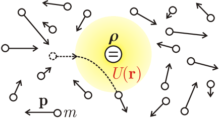
Figure 1: Open dynamics of the system (large circle) with density operator $\varrho$ due to interaction with a diluted gas (small circles).

II The low density limit for the fully quantum model

II.1 Gas of particles with no internal degrees of freedom

Consider an ideal gas of $N$ nonrelativistic particles each of mass $m$ moving in $\mathbb{R}^{3}$. Thermal state of such gas is described by the density operator

$$\varrho_{E}=\varrho_{1}^{\otimes N},\quad\varrho_{1}=\frac{(2\pi\hbar)^{3}}{V}\int f({\bf p})\ket{\bf p}\bra{\bf p}d^{3}{\bf p},$$ (3)

where $V$ is a volume occupied by gas, $\ket{{\bf p}}$ is a single-particle state with the definite momentum ${\bf p}$ such that ${\langle{\bf p}|}{{\bf p}^{\prime}\rangle}=\delta({\bf p}-{\bf p}^{\prime})$, and $f({\bf p})$ is the Maxwell–Boltzmann distribution

$$f({\bf p})=\left(2\pi mkT\right)^{-3/2}\exp\left(-\frac{{\bf p}^{2}}{2mkT}\right).$$ (4)

Here $k$ is the Boltzmann constant and $T$ is the temperature. In the position representation, we have

$${\langle\bf r|}{\bf p\rangle}=(2\pi\hbar)^{-3/2}\exp\left(\frac{i{\bf p}{\bf r}}{\hbar}\right),$$ (5)

so the density operator (3) is properly normalized, namely,

$${\rm tr}[\varrho_{E}]=\left(\int\bra{\bf r}\varrho_{E}\ket{\bf r}d^{3}{\bf r}\right)^{N}=\left(\int f({\bf p})d^{3}{\bf p}\right)^{N}=1.$$ (6)

We consider the gas in the thermodynamic equilibrium with the homogeneous density of particles $n({\bf r})=n$. The density $n$ is expressed through the creation and annihilation operators in coordinate representation, $a^{{\dagger}}({\bf r})$ and $a({\bf r})$, as follows:

$$n=\frac{N}{V}={\rm tr}\left[\varrho_{E}a^{{\dagger}}({\bf r})a({\bf r})\right]=\langle a^{{\dagger}}({\bf r})a({\bf r})\rangle.$$ (7)

In the momentum representation, we have

$$\langle a^{{\dagger}}({\bf p})a({\bf p}^{\prime})\rangle = {\rm tr}\left[\varrho_{E}a^{{\dagger}}({\bf p})a({\bf p}^{\prime})\right]$$ (8)

$$= (2\pi\hbar)^{3}nf({\bf p})\delta({\bf p}-{\bf p}^{\prime}),$$

where $\delta$ is the Dirac delta function (in this case, in a three-dimensional space of momenta).

The Hamiltonian of a single gas particle is $H_{1}=\int\frac{{\bf p}^{2}}{2m}\ket{{\bf p}}\bra{{\bf p}}d^{3}{\bf p}$. Its second quantization gives the environment Hamiltonian

$$H_{E}=\int\frac{{\bf p}^{2}}{2m}a^{{\dagger}}({\bf p})a({\bf p})d^{3}{\bf p}.$$ (9)

Let $H_{S}=\sum_{k}\epsilon_{k}\ket{k}\bra{k}$ be the system Hamiltonian and $H_{S1}$ be the interaction Hamiltonian for the system and a single gas particle. The total interaction Hamiltonian $H_{\rm int}$ is the second quantization of $H_{S1}$. For instance, if $H_{S1}=Q_{S}\otimes U({\bf r})$, then $H_{\rm int}=Q_{S}\otimes\int U({\bf r})a^{{\dagger}}({\bf r})a({\bf r})d^{3}{\bf r}$.

The system and the gas environment altogether evolve in accordance with the von Neumann equation

$$\frac{d\varrho_{S+E}}{dt}=-\frac{i}{\hbar}[H_{S}\otimes I_{E}+I_{S}\otimes H_{E}+H_{\rm int},\varrho_{S+E}]$$ (10)

with the initial condition $\varrho_{S+E}(0)=\varrho_{S}(0)\otimes\varrho_{E}$. The reduced system evolution is obtained by taking the partial trace over environment,

$$\frac{d\varrho_{S}}{dt}={\rm tr}_{E}\left(-\frac{i}{\hbar}[H_{S}\otimes I_{E}+I_{S}\otimes H_{E}+H_{\rm int},\varrho_{S+{E}}]\right).$$ (11)

The fundamental result of the LDL approach dumcke-1985 is that the open dynamics (11) in the limit $n\rightarrow 0$, $t\rightarrow+\infty$, $nt={\rm const.}$, reduces to Eq. (1) with the GKSL generator (2), namely,

$$\frac{d\varrho_{S}}{dt}=-\frac{i}{\hbar}[H_{S}+H_{\rm LS},\varrho_{S}]+{\cal D}[\varrho_{S}].$$ (12)

Importantly, the Lamb shift $H_{\rm LS}$ and the dissipator ${\cal D}$ depend only on the scattering $\hat{T}$-operator for the interaction of the system with one particle of the gas,

$$\hat{T}=H_{S1}\lim_{t\rightarrow\infty}\!\!\! \bigg{\{} \!\!\!\exp\left[-\frac{it}{\hbar}\biggl{(}H_{S}\otimes I_{1}+I_{S}\otimes H_{1}+H_{S1}\biggr{)}\right]$$ (13)

$$\!\!\!\times\exp\left[\frac{it}{\hbar}\biggl{(}H_{S}\otimes I_{1}+I_{S}\otimes H_{1}\biggr{)}\right]\bigg{\}}.$$

Denoting $T(k,{\bf q}|l,{\bf p}):=\bra{k}\otimes\bra{\bf q}\hat{T}\ket{l}\otimes\ket{\bf p}$ and

$$T_{\epsilon}({\bf q},{\bf p})=\sum_{k,l:~{}\epsilon_{k}-\epsilon_{l}=\epsilon}T(k,{\bf q}|l,{\bf p})\ket{k}\bra{l},$$ (14)

the final result is dumcke-1985

$$H_{\rm LS} = (2\pi\hbar)^{3}n\sum_{k,l:\ \epsilon_{k}=\epsilon_{l}}\int d^{3}{\bf p}\,f({\bf p})\,{\rm Re}T(k,{\bf p}|l,{\bf p})\,\ket{k}\bra{l},\quad\,\,\,$$ (15)

$${\cal D}[\varrho_{S}] = (2\pi)^{4}\hbar^{2}n\sum_{\epsilon}\iint d^{3}{\bf p}\,d^{3}{\bf q}\,f({\bf p})\,\delta\left(\frac{{\bf q}^{2}}{2m}-\frac{{\bf p}^{2}}{2m}+\epsilon\right)$$ (16)

$$\times \left[T_{\epsilon}({\bf q},{\bf p})\varrho_{S}T_{\epsilon}^{{\dagger}}({\bf q},{\bf p})-\frac{1}{2}\left\{\varrho_{S},T_{\epsilon}^{{\dagger}}({\bf q},{\bf p})T_{\epsilon}({\bf q},{\bf p})\right\}\right].$$

Here, we restored the physical dimension of the Lamb shift (energy) and the dissipator (frequency) and have taken into account the factor $(2\pi\hbar)^{3}$ from Eq. (8).

In what follows, we consider a modification of the LDL approach for the case of gas particles having also internal degrees of freedom, e.g., spin.

II.2 Gas of particles with internal degrees of freedom

Let $\{\ket{i}\}_{i}$ be an eigenbasis for the internal Hamiltonian of gas particles, $H_{\lambda}=\sum_{i}\lambda_{i}\ket{i}\bra{i}$. Merging the motional and internal degrees of freedom in the notation $\ket{i,{\bf p}}$, we denote the corresponding creation and annihilation operators by

$$a_{i}^{{\dagger}}({\bf p}):=a^{{\dagger}}(i,{\bf p}),\quad a_{i}({\bf p}):=a(i,{\bf p}).$$ (17)

Suppose that the internal state of every gas particle is $\sum_{i}\mu_{i}\ket{i}\bra{i}$. Then the environmental state is $\widetilde{\varrho}_{E}=\widetilde{\varrho}_{1}^{\otimes N}$ with

$$\widetilde{\varrho}_{1}=\frac{(2\pi\hbar)^{3}}{V}\sum_{i}\mu_{i}\int f({\bf p})\ket{i,{\bf p}}\bra{i,{\bf p}}d^{3}{\bf p}.$$ (18)

The single-particle Hamiltonian $\widetilde{H}_{1}:=H_{\lambda}\otimes I_{1}+I_{\lambda}\otimes H_{1}$ represents the sum of internal and kinetic energies, respectively. The second quantized version of $\widetilde{H}_{1}$ is

$$\widetilde{H}_{E}=\sum_{i}\int d^{3}{\bf p}\left(\lambda_{i}+\frac{{\bf p}^{2}}{2m}\right)a_{i}^{{\dagger}}({\bf p})a_{i}({\bf p})$$ (19)

and commutes with $\widetilde{\varrho}_{E}$.

This model allows for including the interaction between the system and the internal degrees of freedom of gas particles during collisions. We consider the interaction Hamiltonian of the form

$$\widetilde{H}_{S1}=F\otimes U({\bf r})=\sum_{k,l,i,j}F_{ki,lj}\ket{k}\bra{l}\otimes\ket{i}\bra{j}\otimes U({\bf r}),$$ (20)

where the operator $F$ describes interaction between internal degrees of freedom of the system and a gas particle, and $U({\bf r})$ determines the strength of this interaction for a given position ${\bf r}$ of the gas particle with respect to the system, see Fig. 2.

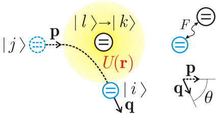
Figure 2: A gas particle with the initial momentum ${\bf p}$ and internal state $\ket{j}$ is scattered to the state with momentum ${\bf q}$ and internal state $\ket{i}$, whereas the system state is changed from $\ket{l}$ to $\ket{k}$. Operator $F$ defines the interaction between internal degrees of freedom of the gas particle and the system, potential $U({\bf r})$ determines the strength of the interaction.

The scattering operator for this model is

$$\widetilde{T}=\widetilde{H}_{S1}\lim_{t\rightarrow\infty}\!\!\! \bigg{\{} \!\!\!\exp\left[-\frac{it}{\hbar}\left(H_{S}\otimes\widetilde{I}_{1}+I_{S}\otimes\widetilde{H}_{1}+\widetilde{H}_{S1}\right)\right]$$ (21)

$$\!\!\!\times\exp\left[\frac{it}{\hbar}\left(H_{S}\otimes\widetilde{I}_{1}+I_{S}\otimes\widetilde{H}_{1}\right)\right]\bigg{\}},$$

where $\widetilde{I}_{1}$ is the identity operator for the gas particle. Denoting $\widetilde{T}(k;i,{\bf q}|l;j,{\bf p}):=\bra{k;i,{\bf q}}\widetilde{T}\ket{l;j,{\bf p}}$ and

$$\widetilde{T}_{\epsilon}(i,{\bf q};j,{\bf p})=\sum_{k,l:~{}\epsilon_{k}-\epsilon_{l}=\epsilon}\widetilde{T}(k;i,{\bf q}|l;j,{\bf p})\ket{k}\bra{l},$$ (22)

the final result for the Lamb shift and dissipator in the LDL master equation is

$$\widetilde{H}_{\rm LS} = (2\pi\hbar)^{3}n\sum_{i}\sum_{k,l:\,\epsilon_{k}=\epsilon_{l}}\mu_{i}$$ (23)

$$\times\int d^{3}{\bf p}\,f({\bf p})\,{\rm Re}\widetilde{T}(k;i,{\bf p}|l;i,{\bf p})\,\ket{k}\bra{l},$$

$$\widetilde{\cal D}[\varrho_{S}] = (2\pi)^{4}\hbar^{2}n\sum_{\epsilon}\sum_{i,j}\mu_{j}\iint d^{3}{\bf p}\,d^{3}{\bf q}\,f({\bf p})\delta\bigg{(}\frac{{\bf q}^{2}}{2m}+\lambda_{i}$$ (24)

$$-\frac{{\bf p}^{2}}{2m}-\lambda_{j}+\epsilon\bigg{)}\bigg{[}\widetilde{T}_{\epsilon}(i,{\bf q};j,{\bf p})\varrho_{S}\widetilde{T}_{\epsilon}^{{\dagger}}(i,{\bf q};j,{\bf p})$$

$$-\frac{1}{2}\left\{\varrho_{S},\widetilde{T}_{\epsilon}^{{\dagger}}(i,{\bf q};j,{\bf p})\widetilde{T}_{\epsilon}(i,{\bf q};j,{\bf p})\right\}\bigg{]}.\qquad$$

II.3 Gas of spin particles in the Born approximation

Consider a gas of particles with degenerate internal degrees of freedom, e.g., spin particles in zero magnetic field. In this case, $\lambda_{i}=0$ for all $i$ and $H_{\lambda}=0$. To further simplify the expression (24), let us also assume that the separation of system energy levels is small as compared to the characteristic kinetic energy of gas particles, i.e. that $|\epsilon_{k}-\epsilon_{l}|\ll\left\langle\frac{{\bf p}^{2}}{2m}\right\rangle$. For instance, this holds if the system is a spin in zero magnetic field. In this case, the collisions are elastic meaning that the energy of incident particles equals the energy of scattered particles. Then $\epsilon$ takes the only zero value, and we simplify the summations: $\sum_{k,l:\,\epsilon_{k}=\epsilon_{l}}=\sum_{k,l}$ and $\widetilde{T}_{0}(i,{\bf q};j,{\bf p})=\sum_{k,l}\widetilde{T}(k;i,{\bf q}|l;j,{\bf p})\ket{k}\bra{l}$. Additionally, we have

$$\delta\left(\frac{{\bf q}^{2}}{2m}-\frac{{\bf p}^{2}}{2m}\right)=\frac{m}{p}\,\delta(q-p),$$ (25)

where we use the notations $q=|{\bf q}|$ and $p=|{\bf p}|$.

To calculate the elements of the $T$-matrix analytically, we consider the first-order Born approximation $\widetilde{T}\approx\widetilde{H}_{S1}$ leading to

$$\widetilde{T}(k;i,{\bf q}|l;j,{\bf p}) \approx F_{ki,lj}\bra{\bf q}U({\bf r})\ket{\bf p}$$ (26)

$$= \frac{F_{ki,lj}}{(2\pi\hbar)^{3}}\int e^{i({\bf p}-{\bf q}){\bf r}/\hbar}U({\bf r})d^{3}{\bf r}.\quad$$

Let $U_{0}$ be the characteristic strength of $U({\bf r})$ and $d$ be the characteristic distance such that $U({\bf r})$ is negligible if $|{\bf r}|>d$. Then the first-order Born approximation is valid for fast particles with $pd\gg\hbar$ if $U_{0}\ll\frac{\hbar p}{md}$ LL . Since the average momentum is $\langle p\rangle=\int|{\bf p}|f({\bf p})d^{3}{\bf p}=\sqrt{8mkT/\pi}$, the first-order Born approximation is valid for fast particles if

$$U_{0}\ll\sqrt{\frac{\hbar^{2}kT}{md^{2}}}.$$ (27)

In the first-order Born approximation, substituting Eq. (26) into the Lamb shift (23) and the dissipator (24) yields

$$\widetilde{H}_{\rm LS}^{\rm LDL} = n\int U({\bf r})d^{3}{\bf r}\sum_{i}\mu_{i}A_{ii},$$ (28)

$$\widetilde{\cal D}^{\rm LDL}[\varrho_{S}] = \Gamma\sum_{i,j}\mu_{j}\left(A_{ij}\varrho_{S}A_{ij}^{{\dagger}}-\frac{1}{2}\left\{\varrho_{S},A_{ij}^{{\dagger}}A_{ij}\right\}\right),\qquad$$ (29)

where we introduced the notations

$$A_{ij} = \sum_{k,l}F_{ki,lj}\ket{k}\bra{l}=I_{S}\otimes\bra{i}\,F\,I_{S}\otimes\ket{j},$$ (30)

$$\Gamma = (2\pi)^{4}\hbar^{2}nm\iint d^{3}{\bf p}\,d^{3}{\bf q}\frac{\,f({\bf p})\,\big{|}\!\bra{\bf q}U({\bf r})\ket{\bf p}\!\big{|}^{2}\,\delta(q-p)}{p}$$

and have taken into account $\int d^{3}{\bf p}f({\bf p})=1$.

Provided the potential $U({\bf r})$ is spherically symmetrical, i.e., $U({\bf r})=V(r)$, $r=|{\bf r}|$, the expression (II.3) can be further simplified. In this case, the Fourier transform $\bra{\bf q}U({\bf r})\ket{\bf p}$ depends only on the absolute value $|{\bf q}-{\bf p}|$, which in turn depends on the scattering angle $\theta$ between ${\bf p}$ and ${\bf q}$. Due to the presence of delta function $\delta(p-q)$ in $\Gamma$, one can set $q=p$ that gives $|{\bf q}-{\bf p}|=2p\sin\frac{\theta}{2}$ and

$$\bra{\bf q}U({\bf r})\ket{\bf p}\Big{|}_{q=p}$$

$$=\frac{1}{(2\pi\hbar)^{2}p\sin\frac{\theta}{2}}\int\limits_{0}^{\infty}V(r)\sin\left(\frac{2pr}{\hbar}\sin\frac{\theta}{2}\right)rdr.$$ (32)

Remembering that the distribution $f({\bf p})$ depends on the absolute value of momentum $p=|{\bf p}|$, we further use the notation $f(p)$ instead of $f({\bf p})$ to refer to Eq. (4). This allows us to first integrate over $d^{3}{\bf q}=q^{2}dq\sin\theta d\theta d\varphi$ and later use the simplified expression $d^{3}{\bf p}=4\pi p^{2}dp$. Introducing a new variable, $\xi=\sin\frac{\theta}{2}$, we have $\sin\theta d\theta=4\xi d\xi$ and finally

$$\Gamma=\frac{32\pi^{2}nm}{\hbar^{2}}\int\limits_{0}^{\infty}f(p)\,p\,dp\int\limits_{0}^{1}\frac{d\xi}{\xi}\left(\int\limits_{0}^{\infty}V(r)\sin\frac{2pr\xi}{\hbar}\,rdr\right)^{2}.$$ (33)

In what follows, we consider the particular cases of analytically tractable potentials $V(r)$ to get the final explicit expression for the dissipator $\widetilde{\cal D}^{\rm LDL}$.

II.3.1 Gaussian potential

Consider Gaussian potential $U({\bf r})=V(r)=U_{0}\exp\left(-\dfrac{r^{2}}{2d^{2}}\right)$. Direct computation yields

$$\int\limits_{0}^{\infty}V(r)\sin\frac{2pr\xi}{\hbar}\,rdr=\frac{\sqrt{2\pi}pd^{3}U_{0}\xi}{\hbar}\exp\left(-\frac{2p^{2}d^{2}\xi^{2}}{\hbar^{2}}\right).$$ (34)

Substituting Eq. (34) into Eq. (33), we get

$$\Gamma=\frac{(2\pi)^{3/2}nmd^{4}U_{0}^{2}}{\hbar^{2}\sqrt{mkT}\left(1+\dfrac{\hbar^{2}}{8md^{2}kT}\right)}.$$ (35)

Since the average momentum $\langle p\rangle=\sqrt{8mkT/\pi}$ satisfies the condition $\langle p\rangle d\gg\hbar$ for fast particles, we neglect the term $\frac{\hbar^{2}}{8md^{2}kT}$ in Eq. (35) and obtain

$$\Gamma\Big{|}_{\rm fast}=\frac{(2\pi)^{3/2}nmd^{4}U_{0}^{2}}{\hbar^{2}\sqrt{mkT}}.$$ (36)

The derived expression is valid if the condition (27) is additionally satisfied.

II.3.2 Spherical square-well potential

Consider the spherical square-well potential $U({\bf r})=V(r)=\left\{\begin{array}[]{ll}U_{0},&r\leq d,\\ 0,&r>d.\\ \end{array}\right.$ Then

$$\int\limits_{0}^{\infty}V(r)\sin\frac{2pr\xi}{\hbar}\,rdr=\frac{\hbar dU_{0}}{2p\xi}\left(\frac{\hbar}{2pd\xi}\sin\frac{2pd\xi}{\hbar}-\cos\frac{2pd\xi}{\hbar}\right).$$ (37)

Substituting Eq. (37) into Eq. (33), we get a rather complicated expression, which is simplified for fast particles with $\langle p\rangle d\gg\hbar$ as follows:

$$\Gamma\Big{|}_{\rm fast}=\frac{2\sqrt{2\pi}nmd^{4}U_{0}^{2}}{\hbar^{2}\sqrt{mkT}}.$$ (38)

Note that the obtained result is derived within the first-order Born approximation that is valid if the condition (27) is satisfied.

III Semiclassical collision model

III.1 Collision model with a finite interaction time

In conventional collision models rau-1963 ; scarani-2002 , the quantum system sequentially interacts with environmental particles, whose only degrees of freedom are internal. The system interacts with each environmental particle only once, and the initial state of all environment particles is $\left(\sum_{i}\mu_{i}\ket{i}\bra{i}\right)^{\otimes N}$. Each collision lasts for a finite time $\tau$. In between the collisions, the system evolves unitarily with its Hamiltonian $H_{S}$. Denote by $t_{\rm free}$ the intercollision time. Then the frequency of collisions equals $(t_{\rm free}+\tau)^{-1}$, see Fig. 3.

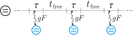
Figure 3: Collision model with impact time $\tau$ and free propagation time $t_{\rm free}$. The system-particle Hamiltonian during the collision is $gF$.

Let $gF$ be the system-particle Hamiltonian during the collision, where $g$ is the characteristic strength. This implies that one can neglect the effect of the system Hamiltonian during the collision, which is justified if $\tau\|[H_{S}\otimes I,F]\|\ll\hbar\|F\|$. In particular, it takes place if $|\epsilon_{k}-\epsilon_{l}|\tau\ll\hbar$. Assuming $g\tau\ll\hbar$, we obtain the following master equation for the system:

$$\!\!\!\!\!\!\!\!\!\!\frac{d\varrho_{S}}{dt}=-\frac{i}{\hbar(t_{\rm free}+\tau)}\left[t_{\rm free}H_{S}+g\tau\sum_{i}\mu_{i}A_{ii},\varrho_{S}\right]$$

$$\!\!\!\!\!\!\!\!\!\!+\frac{g^{2}\tau^{2}}{\hbar^{2}(t_{\rm free}+\tau)}\sum_{i,j}\mu_{j}\left(A_{ij}\varrho_{S}A_{ij}^{{\dagger}}-\frac{1}{2}\left\{\varrho_{S},A_{ij}^{{\dagger}}A_{ij}\right\}\right),\qquad$$ (39)

where the operators $A_{ij}$ are expressed through $F$ exactly as in Eq. (30).

If $\tau\gg t_{\rm free}$, then the obtained master equation is valid in the limit $g\tau\rightarrow 0$, $g^{2}\tau\rightarrow{\rm const.}$ giovannetti-2012 ; lorenzo-2017 ; luchnikov-2017 . If $\tau\ll t_{\rm free}$, then Eq. (III.1) reduces to

$$\frac{d\varrho_{S}}{dt}=-\frac{i}{\hbar}\left[H_{S}+\frac{g\tau}{t_{\rm free}}\sum_{i}\mu_{i}A_{ii},\varrho_{S}\right]$$

$$+\frac{g^{2}\tau^{2}}{\hbar^{2}t_{\rm free}}\sum_{i,j}\mu_{j}\left(A_{ij}\varrho_{S}A_{ij}^{{\dagger}}-\frac{1}{2}\left\{\varrho_{S},A_{ij}^{{\dagger}}A_{ij}\right\}\right),\qquad$$ (40)

and is valid if $g\tau\ll\hbar$.

Finally, consider an ensemble of particles with various values of the parameter $g\tau$ that appear with various frequencies $t_{\rm free}^{-1}$. Collisions with such an ensemble result in the Lamb shift and the dissipator as follows:

$$\!\!\!\!\!\!\!\!\!\!H_{\rm LS}=\left\langle\frac{g\tau}{t_{\rm free}}\right\rangle\sum_{i}\mu_{i}A_{ii},$$ (41)

$$\!\!\!\!\!\!\!\!\!\!{\cal D}[\varrho_{S}]=\left\langle\frac{g^{2}\tau^{2}}{\hbar^{2}t_{\rm free}}\right\rangle\sum_{i,j}\mu_{j}\left(A_{ij}\varrho_{S}A_{ij}^{{\dagger}}-\frac{1}{2}\left\{\varrho_{S},A_{ij}^{{\dagger}}A_{ij}\right\}\right).$$

III.2 Collision model for gas particles

In the semiclassical collision model, gas particles move along the classical trajectories, whereas their internal degrees of freedom are quantum. We consider a low density gas ($nd^{3}\ll 1$), so that the collisions are rather rare and we can neglect the events when two or more gas particles are simultaneously in the volume $\sim d^{3}$ nearby the system. It means that the effective interaction time $\tau$ is much less than the intercollision time $t_{\rm free}$.

Consider an itinerant gas particle with the given trajectory ${\bf r}(t)$ that moves in the potential $U({\bf r})$ with characteristic length $d$. Define the effective collision time $\tau$ through

$$U_{0}\tau=\int_{-\infty}^{+\infty}U\big{(}{\bf r}(t)\big{)}dt,$$ (43)

where $U_{0}$ is the characteristic strength of the potential $U({\bf r})$. Then a single collision with the interaction Hamiltonian (20) results in the unitary operator $W=\exp(-\frac{i}{\hbar}U_{0}F\tau)$ that acts on the internal degrees of freedom of the system and the itinerant gas particle. Therefore, $U_{0}\tau$ plays the same role as $g\tau$ in Sec. III.1. Note that despite the fact that a particle enters the interaction region $|{\bf r}|<d$ for a finite period $(t_{\rm in},t_{\rm out})$, we can still use definition (43) because the potential $U({\bf r})$ is negligible when a gas particle is outside the interaction region.

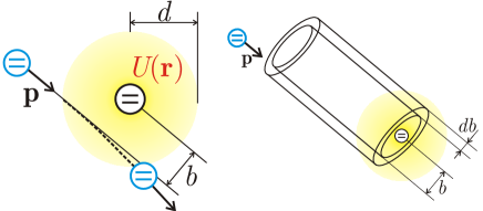
Figure 4: The impact parameter $b$. The classical trajectories are approximated by straight lines for fast gas particles (left). The volume of particles with momentum ${\bf p}$ and impact parameter $b-(b+db)$ that reach the interaction region within time $t$, is $dV=2\pi b\,db\times pt/m$ (right).

If the interaction strength between the system and a particle ($\sim U_{0}$) is small as compared to the kinetic energy of a gas particle ($\sim kT$), then we can neglect the curvature of trajectories and approximate them by straight lines, see Fig. 4. As before, we additionally assume that $U({\bf r})=V(r)$, i.e., the potential is spherically symmetrical. Within such an approximation, $U_{0}\tau$ depends on the absolute value of particle momentum, $p$, and the impact parameter $b$ (see Fig. 4):

$$U_{0}\tau=\int_{-\infty}^{+\infty}V\left(\sqrt{b^{2}+\tfrac{p^{2}t^{2}}{m^{2}}}\right)dt.$$ (44)

Consider particles with momenta ${\bf p}-({\bf p}+d{\bf p})$. The number of particles that would pass through the interaction region with impact parameters $b-(b+db)$ within time period $t$ equals $ndVf({\bf p})d^{3}{\bf p}$, where $dV=2\pi b\,db\times pt/m$ is the corresponding volume, see Fig. 4. Therefore, the collision rate for such particles reads

$$\frac{1}{t_{\rm free}}=\frac{n\times 2\pi b\,db\times pf({\bf p})d^{3}{\bf p}}{m}=\frac{8\pi^{2}nbp^{3}f(p)\,db\,dp}{m}.$$ (45)

Using the results of Sec. III.1, we readily find the Lamb shift and the dissipator in the semiclassical collision model:

$$H_{\rm LS}^{\rm CM}=\left\langle\frac{U_{0}\tau}{t_{\rm free}}\right\rangle\sum_{i}\mu_{i}A_{ii},$$ (46)

$${\cal D}^{\rm CM}=\left\langle\frac{U_{0}^{2}\tau^{2}}{\hbar^{2}t_{\rm free}}\right\rangle\sum_{i,j}\mu_{j}\left(A_{ij}\varrho_{S}A_{ij}^{{\dagger}}-\frac{1}{2}\left\{\varrho_{S},A_{ij}^{{\dagger}}A_{ij}\right\}\right).$$

Here

$$\left\langle\frac{U_{0}\tau}{t_{\rm free}}\right\rangle=\int_{0}^{\infty}db\int_{0}^{\infty}dp\frac{8\pi^{2}nbp^{3}f(p)}{m}$$

$$\qquad\quad\times\int_{-\infty}^{+\infty}V\left(\sqrt{b^{2}+\tfrac{p^{2}t^{2}}{m^{2}}}\right)dt,$$ (48)

$$\left\langle\frac{U_{0}^{2}\tau^{2}}{\hbar^{2}t_{\rm free}}\right\rangle=\int_{0}^{\infty}db\int_{0}^{\infty}dp\frac{8\pi^{2}nbp^{3}f(p)}{\hbar^{2}m}$$

$$\qquad\quad\times\left[\int_{-\infty}^{+\infty}V\left(\sqrt{b^{2}+\tfrac{p^{2}t^{2}}{m^{2}}}\right)dt\right]^{2}.$$ (49)

Since $\tau\sim\frac{md}{\langle p\rangle}\sim\sqrt{\frac{md^{2}}{kT}}$ and $t_{\rm free}\sim\frac{m}{nd^{2}\langle p\rangle}$, the derived formulas are valid if $nd^{3}\ll 1$ (approximation of rare collisions, $\tau\ll t_{\rm free}$), $|\epsilon_{k}-\epsilon_{l}|\sqrt{\frac{md^{2}}{kT}}\ll\hbar$ and $U_{0}\sqrt{\frac{md^{2}}{kT}}\ll\hbar$ (stroboscopic approximation), $kT\gg U_{0}$ (approximation of straight trajectories).

In what follows, we consider particular cases of analytically tractable potentials $V(r)$ to get the explicit expressions for Eqs. (III.2) and (III.2).

III.2.1 Gaussian potential

If $U({\bf r})=V(r)=U_{0}\exp\left(-\dfrac{r^{2}}{2d^{2}}\right)$, then

$$\int_{-\infty}^{+\infty}V\left(\sqrt{b^{2}+\tfrac{p^{2}t^{2}}{m^{2}}}\right)dt=\frac{\sqrt{2\pi}mdU_{0}}{p}\exp\left(-\frac{b^{2}}{2d^{2}}\right).$$ (50)

Substituting Eq. (50) into Eqs. (III.2) and (III.2), we get

$$\left\langle\frac{U_{0}\tau}{t_{\rm free}}\right\rangle=(2\pi)^{3/2}nd^{3}U_{0},$$ (51)

$$\left\langle\frac{U_{0}^{2}\tau^{2}}{\hbar^{2}t_{\rm free}}\right\rangle=\frac{(2\pi)^{3/2}nmd^{4}U_{0}^{2}}{\hbar^{2}\sqrt{mkT}}.$$ (52)

III.2.2 Spherical square-well potential

If $U({\bf r})=V(r)=\left\{\begin{array}[]{ll}U_{0},&r\leq d,\\ 0,&r>d,\\ \end{array}\right.$ then

$$\int_{-\infty}^{+\infty}V\left(\sqrt{b^{2}+\tfrac{p^{2}t^{2}}{m^{2}}}\right)dt=\left\{\begin{array}[]{ll}\frac{2mU_{0}}{p}\sqrt{d^{2}-b^{2}},&b\leq d,\\ 0,&b>d.\\ \end{array}\right.$$ (53)

Substituting Eq. (53) into Eqs. (III.2) and (III.2), we get

$$\left\langle\frac{U_{0}\tau}{t_{\rm free}}\right\rangle=\frac{4\pi}{3}nd^{3}U_{0},$$ (54)

$$\left\langle\frac{U_{0}^{2}\tau^{2}}{\hbar^{2}t_{\rm free}}\right\rangle=\frac{2\sqrt{2\pi}nmd^{4}U_{0}^{2}}{\hbar^{2}\sqrt{mkT}}.$$ (55)

IV Comparison of the two approaches

IV.1 Comparison in the high temperature limit

In Secs. II and III, the two different approaches are presented for the derivation of the GKSL master equation for a spin system interacting with a diluted gas of spin particles. In the low density limit of the fully quantum approach, the generator of the master equation is defined by formulas (28) and (29). In the semiclassical collision model, the generator of the master equation is defined by formulas (46) and (III.2).

The first observation is that both generators are expressed through the same operators $A_{ij}$ and have identical operator structure.

Second, the Lamb shifts (28) and (46) exactly coincide because by the change of variables $z=pt/m$ in Eq. (III.2) we extract $\int_{0}^{\infty}4\pi^{2}p^{2}f(p)dp=1$ and get the following integral in cylindrical coordinates:

$$\left\langle\frac{U_{0}\tau}{t_{\rm free}}\right\rangle = n\int_{0}^{\infty}2\pi bdb\int_{-\infty}^{+\infty}V\left(\sqrt{b^{2}+z^{2}}\right)dz$$ (56)

$$= n\int U({\bf r})d^{3}{\bf r}.$$

Third, the dissipators (29) and (III.2) generally do not exactly coincide because $\Gamma\neq\left\langle\frac{U_{0}^{2}\tau^{2}}{\hbar^{2}t_{\rm free}}\right\rangle$ for finite temperatures, cf. Eqs. (35) and (52). However, for the considered examples of Gaussian and spherical square-well potentials surprisingly $\Gamma|_{\rm fast}=\left\langle\frac{U_{0}^{2}\tau^{2}}{\hbar^{2}t_{\rm free}}\right\rangle$. In fact, if the average kinetic energy $kT\gg\frac{\hbar^{2}}{md^{2}}$, then the gas particles are fast and the dominant scattering angles satisfy $\theta\lesssim\frac{\hbar}{pd}$, Ref. LL . In this case, $\xi=\sin\frac{\theta}{2}\lesssim\frac{\hbar}{2pd}$ and

$$\int_{0}^{1}\frac{d\xi}{\xi}\left(\int_{0}^{\infty}V(r)\sin\frac{2pr\xi}{\hbar}\,rdr\right)^{2}$$

$$\approx\int_{0}^{\frac{\hbar}{2pd}}\frac{d\xi}{\xi}\left(\int_{0}^{d}V(r)\sin\frac{2pr\xi}{\hbar}\,rdr\right)^{2}$$

$$\approx\int_{0}^{\frac{\hbar}{2pd}}\frac{d\xi}{\xi}\left(\int_{0}^{d}V(r)\frac{2pr\xi}{\hbar}\,rdr\right)^{2}$$

$$=\frac{1}{2d^{2}}\left(\int_{0}^{d}V(r)r^{2}dr\right)^{2}\sim U_{0}^{2}d^{4}.$$ (57)

The obtained estimation is of the same order as the collision model expression,

$$\int_{0}^{\infty}b\,db\left[\int V(\sqrt{b^{2}+z^{2}})dz\right]^{2}\sim U_{0}^{2}d^{4}.$$ (58)

Therefore, $\Gamma\sim\left\langle\frac{U_{0}^{2}\tau^{2}}{\hbar^{2}t_{\rm free}}\right\rangle$ if $kT\gg\frac{\hbar^{2}}{md^{2}}$.

Fourth, in the limit of infinite temperature the dissipators in the low density approach and the collision model exactly coincide for spherical potentials $U({\bf r})=V(r)$, i.e.,

$$\lim_{T\rightarrow\infty}\frac{\Gamma}{\left\langle\frac{U_{0}^{2}\tau^{2}}{\hbar^{2}t_{\rm free}}\right\rangle}=1.$$ (59)

To prove Eq. (59) we rewrite the integral $\int_{-\infty}^{+\infty}V\left(\sqrt{b^{2}+z^{2}}\right)dz=2\int_{b}^{\infty}V(r)\frac{r\,dr}{\sqrt{r^{2}-b^{2}}}$ which yields

$$\int_{0}^{\infty}b\,db\left[\int_{-\infty}^{+\infty}V\left(\sqrt{b^{2}+z^{2}}\right)dz\right]^{2}$$

$$=4\int\limits_{0}^{\infty}b\,db\int\limits_{0}^{\infty}dr\int\limits_{0}^{\infty}dr^{\prime}V(r)V(r^{\prime})rr^{\prime}f(b,r)f(b,r^{\prime}),\qquad$$ (60)

where $f(b,r)=\left\{\begin{array}[]{ll}0&\text{if~{}}r\leq b,\\ \frac{1}{\sqrt{r^{2}-b^{2}}}&\text{if~{}}r>b.\\ \end{array}\right.$ Since

$$\int_{0}^{\infty}b\,db\,f(b,r)f(b,r^{\prime})=\int_{0}^{\min(r,r^{\prime})}\frac{b\,db}{\sqrt{(r^{2}-b^{2})(r^{\prime 2}-b^{2})}}$$

$$=\frac{1}{2}\ln\frac{r+r^{\prime}}{|r-r^{\prime}|},$$ (61)

we get the following expression in the collision model:

$$\left\langle\frac{U_{0}^{2}\tau^{2}}{\hbar^{2}t_{\rm free}}\right\rangle=\frac{16\pi^{2}nm}{\hbar^{2}}\int_{0}^{\infty}f(p)\,p\,dp$$

$$\qquad\times\int_{0}^{\infty}dr\int_{0}^{\infty}dr^{\prime}V(r)V(r^{\prime})rr^{\prime}\ln\frac{r+r^{\prime}}{|r-r^{\prime}|}.$$ (62)

On the other hand, in the low density approach, Eq. (33) can be rewritten in the form

$$\Gamma=\frac{32\pi^{2}nm}{\hbar^{2}}\int\limits_{0}^{\infty}f(p)\,p\,dp\int\limits_{0}^{\infty}dr\int\limits_{0}^{\infty}dr^{\prime}\,V(r)V(r^{\prime})rr^{\prime}K(r,r^{\prime}),$$ (63)

where the kernel

$$K(r,r^{\prime})=\int\limits_{0}^{1}\frac{d\xi}{\xi}\sin\frac{2pr\xi}{\hbar}\sin\frac{2pr^{\prime}\xi}{\hbar}\xrightarrow[]{p\rightarrow\infty}\frac{1}{2}\ln\frac{r+r^{\prime}}{|r-r^{\prime}|}.$$ (64)

As the limit $p\rightarrow\infty$ is equivalent to the high temperature limit $T\rightarrow\infty$, we see that Eqs. (IV.1) and (63) coincide when $T\rightarrow\infty$, which leads to Eq. (59).

Fifth, the applicability of the first-order Born approximation for fast particles in the low-density-limit approach, Eq. (27), is equivalent to the condition of stroboscopic approximation in the collision model, $g\tau\ll\hbar\Leftrightarrow U_{0}\sqrt{\frac{md^{2}}{kT}}\ll\hbar$.

Sixth, if both conditions $kT\gg\frac{\hbar^{2}}{md^{2}}$ (fast particles) and $U_{0}\sqrt{\frac{md^{2}}{kT}}\ll\hbar$ (Born approximation and stroboscopic approximation) are satisfied, then automatically $kT\gg U_{0}$, i.e., the approximation of straight trajectories is justified in the collision model.

Finally, we conclude that both the low density limit approach and the collision model provide very similar predictions for the reduced dynamics of the spin system ($\epsilon_{k}=\epsilon_{l}$, $\lambda_{i}=0$) if $nd^{3}\ll 1$, $kT\gg\frac{\hbar^{2}}{md^{2}}$, and $U_{0}\ll\sqrt{\frac{\hbar^{2}kT}{md^{2}}}$.

IV.2 Estimation of difference for finite temperature

Let us analyze the difference between the two approaches when lowering the gas temperature. We consider a spherical square-well potential, for which the quantitative estimation of the discrepancy becomes tractable.

In the LDL approach, lowering the velocity of gas particles can be taken into account by considering the second-order perturbation of the scattering operator, $\widetilde{T}=F\otimes U({\bf r})+F\otimes U({\bf r})G_{0}^{(+)}(E)F\otimes U({\bf r})$, where $G_{0}^{(+)}(E)$ is the retarded Green operator for Hamiltonian $H_{S}\otimes\widetilde{I}_{1}+I_{S}\otimes\widetilde{H}_{1}$, $E=\frac{p^{2}}{2m}$. Provided $kT\gg\frac{\hbar^{2}}{md^{2}}$, we find the matrix element $\widetilde{T}(k;i,{\bf p}|l;i,{\bf p})$ and calculate the corrected Lamb shift:

$$\widetilde{H}_{\rm LS}^{\rm LDL}=\frac{4\pi}{3}nd^{3}U_{0}\sum_{i,k,l}\mu_{i}\left(F_{ki,li}-\frac{2U_{0}}{kT}(F^{2})_{ki,li}\right)\ket{k}\bra{l}.$$ (65)

Finite values of $\frac{kTmd^{2}}{\hbar^{2}}$ lead to the exponentially small relative error in the Lamb shift of the order of $\frac{\hbar}{d\sqrt{mkT}}\exp(-\frac{kTmd^{2}}{\hbar^{2}})$ as a result of approximate integration

$$\int_{|{\bf r}^{\prime}|\leq d}d^{3}{\bf r}^{\prime}\int d^{3}{\bf p}\,f({\bf p})\,\frac{e^{i|{\bf r}-{\bf r}^{\prime}|p/\hbar}}{|{\bf r}-{\bf r}^{\prime}|}$$

$$\approx\int_{{\bf r}^{\prime}\in\mathbb{R}^{3}}d^{3}{\bf r}^{\prime}\int d^{3}{\bf p}\,f({\bf p})\,\frac{e^{i|{\bf r}-{\bf r}^{\prime}|p/\hbar}}{|{\bf r}-{\bf r}^{\prime}|}.$$ (66)

We see that the Lamb shifts $\widetilde{H}_{\rm LS}^{\rm LDL}$ and $H_{\rm LS}^{\rm CM}=\left\langle\frac{U_{0}\tau}{t_{\rm free}}\right\rangle\sum_{i,k,l}\mu_{i}F_{ki,li}$ have different operator structure in general. If $\left\langle\frac{U_{0}\tau}{t_{\rm free}}\right\rangle$ is given by Eq. (54), then the relative error

$$\frac{\|\widetilde{H}_{\rm LS}^{\rm LDL}-H_{\rm LS}^{\rm CM}\|}{nd^{3}|U_{0}|\,\|F\|}$$

$$\sim\max\left[\frac{|U_{0}|\,\|F\|}{kT},\frac{\hbar}{d\sqrt{mkT}}\exp\left(-\frac{kTmd^{2}}{\hbar^{2}}\right)\right].$$ (67)

As far as the dissipator in the LDL approach is concerned, the small parameter $\frac{\hbar^{2}}{kTmd^{2}}$ contributes linearly already in the first-order Born approximation [cf. Eq. (35) for the Gaussian potential]. In fact, for a spherical square-well potential we have

$$\int_{0}^{1}\frac{d\xi}{\xi}\left(\int_{0}^{\infty}V(r)\sin\frac{2pr\xi}{\hbar}\,rdr\right)^{2}=\frac{\hbar^{4}U_{0}^{2}}{128p^{3}}$$

$$\times\left(\frac{32p^{4}d^{4}}{\hbar^{4}}-\frac{8p^{2}d^{2}}{\hbar^{2}}-1+\cos\frac{4pd}{\hbar}+\frac{4pd}{\hbar}\sin\frac{4pd}{\hbar}\right)$$

$$\approx\frac{U_{0}^{2}d^{4}}{4}\left[1-\exp\left(-\frac{8p^{2}d^{2}}{9\hbar^{2}}\right)\right],$$ (68)

where the latter approximation provides an interpolation between asymptotics $\frac{2p^{2}U_{0}^{2}d^{6}}{9\hbar^{2}}$ for $\frac{pd}{\hbar}\ll 1$ and $\frac{U_{0}^{2}d^{4}}{4}$ for $\frac{pd}{\hbar}\gg 1$ and has the maximum relative error 4.21% for $\frac{pd}{\hbar}=5.03$. Substituting (68) into (33), we get

$$\Gamma=\frac{2\sqrt{2\pi}nmd^{4}U_{0}^{2}}{\hbar^{2}\sqrt{mkT}}\left(1-\frac{9\hbar^{2}}{16kTmd^{2}}\right).$$ (69)

Similarly to the case of the Lamb shift, we expect that the second order perturbation with respect to the small parameter $\frac{|U_{0}|}{kT}$ in the LDL approach would result in the jump operators that are different from the jump operators in the collision model. Therefore, the relative discrepancy in dissipators is estimated as

$$\frac{\|\widetilde{\cal D}^{\rm LDL}[\varrho]-{\cal D}^{\rm CM}[\varrho]\|}{\frac{nmd^{4}U_{0}^{2}\|F\|^{2}}{\hbar^{2}\sqrt{mkT}}}\sim\frac{1}{kT}\max\left(|U_{0}|\|F\|,\frac{\hbar^{2}}{md^{2}}\right).$$ (70)

It is also possible to slightly adapt the CM approach to allow for lowering velocity of gas particles by considering a perturbation of their trajectories from straight lines caused by a state-dependent potential $\langle F\rangle U({\bf r})$, where $\langle F\rangle={\rm tr}[F\sum_{i}\mu_{i}\ket{i}\bra{i}\otimes\varrho_{S}]=\sum_{i}\mu_{i}{\rm tr}[A_{ii}\varrho_{S}]$. For a spherical square-well potential with negative $\langle F\rangle U_{0}$ the perturbed trajectory consists of 3 line segments. The angle of incidence $\alpha$ and the angle of refraction $\beta$ at the first vertex satisfy the relation $p\sin\alpha=p^{\prime}\sin\beta$, where $p$ and $p^{\prime}=\sqrt{p^{2}+2m\langle F\rangle|U_{0}|}$ are the momenta of the particle outside and inside of the region $|{\bf r}|\leq d$, respectively. Additionally, the angle of incidence is related to the impact parameter $b$ by formula $\sin\alpha=\frac{b}{d}$. The effective collision time

$$\tau=\frac{2md\cos\beta}{p^{\prime}}=\frac{2m\sqrt{(d^{2}-b^{2})p^{2}+2m\langle F\rangle|U_{0}|d^{2}}}{p^{2}+2m\langle F\rangle|U_{0}|}.$$ (71)

Using the exact expression (71) for $\tau$, we find the coefficients $\left\langle\frac{U_{0}\tau}{t_{\rm free}}\right\rangle$ and $\left\langle\frac{U_{0}^{2}\tau^{2}}{\hbar^{2}t_{\rm free}}\right\rangle$ in the Lamb shift (46) and the dissipator (III.2) in the modified semiclassical collision model. The first order expansion of these coefficients with respect to small parameter $\frac{|U_{0}|}{kT}$ reads

$$\!\!\!\!\!\!\!\!\!\!\left\langle\frac{U_{0}\tau}{t_{\rm free}}\right\rangle=\frac{4\pi}{3}nd^{3}U_{0}\left[1-\frac{\langle F\rangle U_{0}}{kT}+o\left(\frac{\langle F\rangle|U_{0}|}{kT}\right)\right],$$ (72)

$$\!\!\!\!\!\!\!\!\!\!\left\langle\frac{U_{0}^{2}\tau^{2}}{\hbar^{2}t_{\rm free}}\right\rangle=\frac{2\sqrt{2\pi}nmd^{4}U_{0}^{2}}{\hbar^{2}\sqrt{mkT}}\left[1+\frac{\langle F\rangle U_{0}}{kT}+o\left(\frac{\langle F\rangle|U_{0}|}{kT}\right)\right].$$

We see that such a non-linear modification of the collision model provides a better agreement between $\widetilde{H}_{\rm LS}^{\rm LDL}$ and $H_{\rm LS}^{\rm CM}$ and between $\widetilde{\cal D}^{\rm LDL}$ and ${\cal D}^{\rm CM}$ for some states $\varrho_{S}$ and operators $F$, however, the discrepancy between the two approaches is still given by formulas (IV.2) and (70) in general.

V Conclusions

We developed and compared two approaches to the analysis of the open quantum system dynamics induced by interaction of the spin-like system with a dilute gas of spin-like particles with internal degrees of freedom: the low density limit in the fully quantum scenario and the semiclassical collision model. We derived GKSL master equations for a specific class of system-particle interaction Hamiltonians of the form $\widetilde{H}_{S1}=F\otimes U({\bf r})$, however, the results remain valid for a general spin-dependent scattering process with the interaction Hamiltonian $\widetilde{H}_{S1}=\sum_{i,j,k,l}\ket{k}\bra{l}\otimes\ket{i}\bra{j}\otimes F_{ki,lj}({\bf r})$. Using the first-order Born approximation in the fully quantum treatment, the simplified expressions for the Lamb shift (28) and the dissipator (29) were derived. In the semiclassical collision model, we used the approximation of straight trajectories and the stroboscopic approximation to get the Lamb shift (46) and the dissipator (III.2). We proved equivalence of the Lamb shifts in both approaches and found that both dissipators (29) and (III.2) qualitatively coincide for finite temperatures and quantitatively coincide in the limit $T\rightarrow\infty$. The illustrative examples of Gaussian and spherical square-well potentials are considered, for which the dissipators (29) and (III.2) are compared in the case of fast particles up to the second order of the scattering potential $F\otimes U({\bf r})$. The sufficient conditions for the two approaches to give the same master equation are $nd^{3}\ll 1$, $kT\gg\frac{\hbar^{2}}{md^{2}}$, and $U_{0}\ll\sqrt{\frac{\hbar^{2}kT}{md^{2}}}$.

- (1) H.-P. Breuer and F. Petruccione, The Theory of Open Quantum Systems (Oxford University Press, Oxford, 2002).
- (2) H. Schoeller, Dynamics of open quantum systems, arXiv:1802.10014 (2018).
- (3) P. Cui, X.-Q. Li, J. Shao, and Y. Yan, Quantum transport from the perspective of quantum open systems, Phys. Lett. A 357, 449 (2006).
- (4) N. W. Talarico, S. Maniscalco, and N. Lo Gullo, A scalable numerical approach to the solution of the Dyson equation for the non-equilibrium single-particle Green’s function, Phys. Status Solidi B 256, 1800501 (2019).
- (5) L. Valkunas, D. Abramavicius, and T. Mancal, Molecular Excitation Dynamics and Relaxation: Quantum Theory and Spectroscopy (Wiley, New York, 2013).
- (6) C. L. Degen, F. Reinhard, and P. Cappellaro, Quantum sensing, Rev. Mod. Phys. 89, 035002 (2017).
- (7) M. M. Wilde, Quantum Information Theory (Cambridge University Press, Cambridge, England, 2017).
- (8) M. A. Nielsen and I. L. Chuang, Quantum Computation and Quantum Information (Cambridge University Press, Cambridge, England, 2000).
- (9) S. N. Filippov, Quantum mappings and characterization of entangled quantum states, J. Math. Sci. 241, 210 (2019).
- (10) S. J. Glaser, U. Boscain, T. Calarco, C. P. Koch, W. Köckenberger, R. Kosloff, I. Kuprov, B. Luy, S. Schirmer, T. Schulte-Herbrüggen, D. Sugny, and F. K. Wilhelm, Training Schrödinger’s cat: quantum optimal control, Eur. Phys. J. D 69, 279 (2015).
- (11) Á. Rivas, S. F. Huelga, and M. B. Plenio, Quantum non-Markovianity: characterization, quantification and detection, Rep. Prog. Phys. 77, 094001 (2014).
- (12) H.-P. Breuer, E.-M. Laine, J. Piilo, and B. Vacchini, Colloquium: Non-Markovian dynamics in open quantum systems, Rev. Mod. Phys. 88, 021002 (2016).
- (13) I. de Vega and D. Alonso, Dynamics of non-Markovian open quantum systems, Rev. Mod. Phys. 89, 015001 (2017).
- (14) F. Benatti, D. Chruściński, and S. Filippov, Tensor power of dynamical maps and positive versus completely positive divisibility, Phys. Rev. A 95, 012112 (2017).
- (15) S. N. Filippov and D. Chruściński, Time deformations of master equations, Phys. Rev. A 98, 022123 (2018).
- (16) L. Li, M. J. W. Hall, and H. M. Wiseman, Concepts of quantum non-Markovianity: A hierarchy, Phys. Rep. 759, 1 (2018).
- (17) I. A. Luchnikov, S. V. Vintskevich, H. Ouerdane, and S. N. Filippov, Simulation complexity of open quantum dynamics: Connection with tensor networks, Phys. Rev. Lett. 122, 160401 (2019).
- (18) L. van Hove, Quantum-mechanical perturbations giving rise to a statistical transport equation, Physica 21, 517 (1954).
- (19) E. B. Davies, Markovian master equations, Commun. Math. Phys. 39, 91 (1974).
- (20) H. Spohn and J. L. Lebowitz, Irreversible thermodynamics for quantum systems weakly coupled to thermal reservoirs, Adv. Chem. Phys. 38, 109 (1978).
- (21) L. Accardi, A. Frigerio, and Y. G. Lu, The weak coupling limit as a quantum functional central limit, Comm. Math. Phys. 131, 537 (1990).
- (22) P. F. Palmer, The singular coupling and weak coupling limits, J. Math. Phys. 18, 527 (1977).
- (23) V. Gorini, A. Frigerio, M. Verri, A. Kossakowski, and E. C. G. Sudarshan, Properties of quantum Markovian master equations, Rep. Math. Phys. 13, 149 (1978).
- (24) L. Accardi, Y. G. Lu, and I. Volovich, Quantum Theory and Its Stochastic Limit (Springer, Berlin, 2002).
- (25) A. N. Pechen and I. V. Volovich, Quantum multipole noise and generalized quantum stochastic equations, Infinite Dimensional Analysis, Quantum Probability and Related Topics 5, 441 (2002).
- (26) R. Dümcke, The low density limit for an -level system interacting with a free Bose or Fermi gas, Commun. Math. Phys. 97, 331 (1985).
- (27) L. Accardi and Y. G. Lu, The low-density limit of quantum systems, J. Phys. A: Math. Gen. 24, 3483 (1991).
- (28) L. Accardi and Y. Lu, The low density limit in finite temperature case, Nagoya Mathematical Journal 126, 25 (1992).
- (29) S. Rudnicki, R. Alicki, and S. Sadowski, The low-density limit in terms of collective squeezed vectors, J. Math. Phys. 33, 2607 (1992).
- (30) L Accardi, A. N. Pechen, and I. V. Volovich, Quantum stochastic equation for the low density limit, J. Phys. A: Math. Gen. 35, 4889 (2002).
- (31) L. Accardi, A. N. Pechen, and I. V. Volovich, A stochastic golden rule and quantum Langevin equation for the low density limit, Infinite Dimensional Analysis, Quantum Probability and Related Topics 6, 431 (2003).
- (32) A. N. Pechen, Quantum stochastic equation for a test particle interacting with a dilute Bose gas, J. Math. Phys. 45, 400 (2004).
- (33) A. N. Pechen, The multitime correlation functions, free white noise, and the generalized Poisson statistics in the low density limit, J. Math. Phys. 47, 033507 (2006).
- (34) J. Rau, Relaxation phenomena in spin and harmonic oscillator systems, Phys. Rev. 129, 1880 (1963).
- (35) V. Giovannetti and G. M. Palma, Master Equations for Correlated Quantum Channels, Phys. Rev. Lett. 108, 040401 (2012).
- (36) S. Lorenzo, F. Ciccarello, and G. M. Palma, Composite quantum collision models, Phys. Rev. A 96, 032107 (2017).
- (37) I. A. Luchnikov and S. N. Filippov, Quantum evolution in the stroboscopic limit of repeated measurements, Phys. Rev. A 95, 022113 (2017).
- (38) K. Hornberger, Monitoring approach to open quantum dynamics using scattering theory, EPL 77, 50007 (2007).
- (39) K. Hornberger and B. Vacchini, Monitoring derivation of the quantum linear Boltzmann equation, Phys. Rev. A 77, 022112 (2008).
- (40) B. Vacchini and K. Hornberger, Quantum linear Boltzmann equation, Phys. Rep. 478, 71 (2009).
- (41) A. Smirne and B. Vacchini, Quantum master equation for collisional dynamics of massive particles with internal degrees of freedom, Phys. Rev. A 82, 042111 (2010).
- (42) V. Gorini, A. Kossakowski, and E. C. G. Sudarshan, Completely positive dynamical semigroups of -level systems, J. Math. Phys. 17, 821 (1976).
- (43) G. Lindblad, On the generators of quantum dynamical semigroups, Comm. Math. Phys. 48, 119 (1976).
- (44) L. Martinetz, K. Hornberger, and B. A. Stickler, Gas-induced friction and diffusion of rigid rotors, Phys. Rev. E 97, 052112 (2018).
- (45) D. J. Wineland, C. Monroe, W. M. Itano, D. Leibfried, B. E. King, and D. M. Meekhof, Experimental issues in coherent quantum-state manipulation of trapped atomic ions, J. Res. Natl. Inst. Stand. Tech. 103, 259 (1998).
- (46) R. M. Serra, N. G. de Almeida, W. B. da Costa, and M. H. Y. Moussa, Decoherence in trapped ions due to polarization of the residual background gas, Phys. Rev. A 64, 033419 (2001).
- (47) H. Uys, J. D. Perreault, and A. D. Cronin, Matter-wave decoherence due to a gas environment in an atom interferometer, Phys. Rev. Lett. 95, 150403 (2005).
- (48) A. Pechen and H. Rabitz, Teaching the environment to control quantum systems, Phys. Rev. A 73, 062102 (2006).
- (49) A. Pechen and H. Rabitz, Incoherent control of open quantum systems, J. Math. Sci. 199, 695 (2014).
- (50) A. N. Pechen’, Some mathematical problems of control of quantum systems, J. Math. Sci. 241, 185 (2019).
- (51) R. Alicki and S. Kryszewski, Completely positive Bloch-Boltzmann equations, Phys. Rev. A 68, 013809 (2003).
- (52) M. Koniorczyk, Á. Varga, P. Rapčan, and V. Bužek, Quantum homogenization and state randomization in semiquantal spin systems, Phys. Rev. A 77, 052106 (2008).
- (53) G. Rempe, F. Schmidt-Kaler, and H. Walther, Observation of sub-Poissonian photon statistics in a micromaser, Phys. Rev. Lett. 64, 2783 (1990).
- (54) V. Scarani, M. Ziman, P. Štelmachovič, N. Gisin, and V. Bužek, Thermalizing quantum machines: Dissipation and entanglement, Phys. Rev. Lett. 88, 097905 (2002).
- (55) T. Rybár, S. N. Filippov, M. Ziman, and V. Bužek, Simulation of indivisible qubit channels in collision models, J. Phys. B: At. Mol. Opt. Phys. 45, 154006 (2012).
- (56) R. McCloskey and M. Paternostro, Non-Markovianity and system-environment correlations in a microscopic collision model, Phys. Rev. A 89, 052120 (2014).
- (57) S. Kretschmer, K. Luoma, and W. T. Strunz, Collision model for non-Markovian quantum dynamics, Phys. Rev. A 94, 012106 (2016).
- (58) A. Dąbrowska, G. Sarbicki, and D. Chruściński, Quantum trajectories for a system interacting with environment in a single-photon state: Counting and diffusive processes, Phys. Rev. A 96, 053819 (2017).
- (59) S. N. Filippov, J. Piilo, S. Maniscalco, and M. Ziman, Divisibility of quantum dynamical maps and collision models, Phys. Rev. A 96, 032111 (2017).
- (60) F. Ciccarello, Collision models in quantum optics, Quantum Measurements and Quantum Metrology 4, 53 (2017).
- (61) A. Levy, R. Alicki, and R. Kosloff, Quantum refrigerators and the third law of thermodynamics, Phys. Rev. E 85, 061126 (2012).
- (62) R. Kosloff, Quantum thermodynamics: A dynamical viewpoint, Entropy 15, 2100 (2013).
- (63) R. Kosloff, Quantum thermodynamics and open-systems modeling, J. Chem. Phys. 150, 204105 (2019).
- (64) L. D. Landau and E. M. Lifshitz, Quantum Mechanics: Non-Relativistic Theory, Sec. 125 (Pergamon, London, 1965).