Compacted binary trees admit a stretched exponential
Abstract
A compacted binary tree is a directed acyclic graph encoding a binary tree in which common subtrees are factored and shared, such that they are represented only once. We show that the number of compacted binary trees of size grows asymptotically like
where is the largest root of the Airy function. Our method involves a new two parameter recurrence which yields an algorithm of quadratic arithmetic complexity for computing the number of compacted trees up to a given size. We use empirical methods to estimate the values of all terms defined by the recurrence, then we prove by induction that these estimates are sufficiently accurate for large to determine the asymptotic form. Our results also lead to new bounds on the number of minimal finite automata recognizing a finite language on a binary alphabet. As a consequence, these also exhibit a stretched exponential.
Keywords: Airy function, asymptotics, bijection, compacted trees, directed acyclic graphs, Dyck paths, finite languages, minimal automata, stretched exponential.
1 Introduction
Compacted binary trees are a special class of directed acyclic graphs that appear as a model for data structures in the compression of XML documents [5]. Given a rooted binary tree of size , its compacted form can be computed in expected and worst-case time with expected compacted size [16]. Recently, Genitrini, Gittenberger, Kauers, and Wallner solved the reversed question on the asymptotic number of compacted trees under certain height restrictions [17]; however the asymptotic number in the unrestricted case remained elusive. They also solved this problem for a simpler class of trees known as relaxed trees under the same height restrictions. In this paper we show that the counting sequences of (unrestricted) compacted binary trees and of (unrestricted) relaxed binary trees both admit a stretched exponential:
Theorem 1.1.
The number of compacted and relaxed binary trees satisfy for
| and |
where is the largest root of the Airy function defined as the unique function satisfying and .
We believe that there are constants and such that
however, we have been unable to find the exact values of these constants or even prove their existence. Nevertheless, our empirical analysis yields what we believe to be very accurate estimates for and , namely and .
The presence of a stretched exponential term in a sequence counting combinatorial objects is not common, although there are quite a few precedents. One simple example is that of pushed Dyck paths, where Dyck paths of maximum height are given a weight for some . In this case McKay and Beaton determined the weighted number of paths of length up to and including the constant term to be asymptotically given by
where and ; see [18]. For the analogous problem of counting pushed self avoiding walks, Beaton et al. [4] gave a (non-rigorous) probabilistic argument for the presence of a stretched exponential of the form for some . In each of these cases, a stretched exponential appears as part of a compromise between the large height regime in which most paths occur and the small height regime in which the weight is maximized. We will see that a similar compromise occurs in this paper. Another situation in which stretched exponentials have appeared is in cogrowth sequences in groups [14], that is, paths on Cayley graphs which start and end at the same point. In particular, Revelle [25] showed that in the lamplighter group the number of these paths of length behaves like
In the group , Pittet and Saloff-Coste showed that the asymptotics of the cogrowth series contains the slightly more complicated term [24]. Another example comes from the study of pattern avoiding permutations, where Conway, Guttmann, and Zinn-Justin [7, 8] have given compelling numerical evidence that the number of 1324-avoiding permutations of length behaves like
with , , .
As seen by these examples, it is generally quite difficult to prove that a sequence has a stretched exponential in its asymptotics. Part of the difficulty is that a sequence which has a stretched exponential cannot be “very nice”. In particular, the generating function cannot be algebraic, and can only be -finite if it has an irregular singularity [15].
Some explicit examples of -finite generating series with a stretched exponential are known; see e.g. [30, 29, 28]. In these cases Wright uses a saddle-point method to prove the presence of the stretched exponential. To apply this method, one needs to meticulously check various analytic conditions on the generating function, or to bound related integrals in a delicate way. These tasks can be highly non-trivial and require a precise knowledge of the analytic properties of the generating function. For more detail on how to use the saddle-point method to prove stretched exponentials, and further examples, see [15, Chapter VIII].
In lieu of detailed information on the generating function, we find and analyze the following recurrence relation
corresponding to a partial differential equation to which the saddle point method cannot be readily applied. The number of relaxed trees of size is then . We present a method that works directly with a transformed sequence and the respective recurrence relation. We find two explicit sequences and with the same asymptotic form, such that
| (1) |
for all and all large enough. The idea is that and satisfy the recurrence of with the equalities replaced by inequalities, allowing us to prove (1) by induction. In order to find appropriate sequences and , we start by performing a heuristic analysis to conjecture the asymptotic shape of for large . We then prove that the required recursive inequalities hold for sufficiently large using adapted Newton polygons.
The inductive step in the method described above requires that all coefficients in the recurrence be positive. This occurs in the case of relaxed binary trees but not for compacted binary trees. In the latter case, we construct a sandwiching pair of sequences, each determined by a recurrence with positive coefficients, to which our method applies.
As an application, we use our results on relaxed and compacted trees to give new asymptotic upper and lower bounds for the number of minimal deterministic finite automata with states recognizing a finite language on a binary alphabet. These automata are studied in the context of the complexity of regular languages; see [12, 23, 11]. To our knowledge no upper or lower bounds capturing even the exponential term had been proven for this problem. Our bounds are much more accurate, only differing by a polynomial factor, and thereby proving the presence of a stretched exponential term.
As a further extension of our method, some preliminary results show that our approach can be generalized to a -ary version of compacted trees, which in turn settles the enumeration of minimal finite automata recognizing finite languages for an arbitrary alphabet. A follow-up paper in this direction is underway.
In its simplest form, our method applies to two parameter linear recurrences with positive coefficients which may depend on both parameters. We expect, however, that our method could be adapted to handle a much wider range of recurrence relations, potentially involving more than two parameters, negative coefficients and perhaps even some non-linear recurrences. Indeed, we have already seen that it can be adapted to at least one case involving negative coefficients, namely that of counting compacted binary trees.
Plan of the article.
In Section 2 we introduce compacted binary trees and the related relaxed binary trees, and then derive a bijection to Dyck paths with weights on their horizontal steps. In Section 3 we show a heuristic method of how to conjecture the asymptotics and in particular the appearance of a stretched exponential term. Building on these heuristics, we prove exponentially and polynomially tight bounds for the recurrence of relaxed binary trees in Section 4 and of compacted binary trees in Section 5. In Section 6 we show how our results lead to new bounds on minimal acyclic automata on a binary alphabet.
2 A two-parameter recurrence relation
Originally, compacted binary trees arose in a compression procedure in [16] which computes the number of unique fringe subtrees. Relaxed binary trees are then defined by relaxing the uniqueness conditions on compacted binary trees. As we will not need this algorithmic point of view, we directly give the following definition adapted from [17, Definition 3.1 and Proposition 4.3].
Before we define compacted and relaxed binary trees, let us recall some basic definitions. A rooted binary tree is a plane directed connected graph with a distinguished node called the root, in which all nodes have out-degree either or and all nodes other than the root have in-degree , while the root has in-degree . For each vertex with out-degree , the out-going edges are distinguished as a left edge and a right edge. Nodes with out-degree are called leaves, and nodes with out-degree are called internal nodes. All trees in this paper will be rooted and we omit this term in the future.
Definition 2.1 (Relaxed binary tree).
A relaxed binary tree (or simply relaxed tree) of size is a directed acyclic graph obtained from a binary tree with internal nodes, called its spine, by keeping the left-most leaf and turning other leaves into pointers, with each one pointing to a node (internal ones or the left-most leaf) preceding it in postorder.
The counting sequence of relaxed binary trees of size starts as follows:
It corresponds to OEIS A082161 in the On-line Encyclopedia of Integer Sequences.††https://oeis.org There, it first appeared as the counting sequence of the number of deterministic, completely defined, initially connected, acyclic automata with inputs and transient, unlabeled states and a unique absorbing state, yet without specified final states. This is a direct rephrasing of Definition 2.1 in the language of automata theory; for more details see Section 6. Liskovets [23] provided (probably) the first recurrence relations ( used for ) and later Callan [6] showed that they are counted by determinants of Stirling cycle numbers. However, the asymptotics remained an open problem, which we will solve in the present paper.

Using the class of relaxed trees, it is then easy to define the set of compacted trees by requiring the uniqueness of subtrees.
Definition 2.2 (Compacted binary tree).
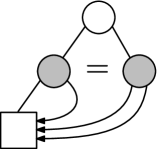
Given a relaxed tree, to each node we can associate a binary tree . We proceed by postorder. If is the left-most leaf, we define . Otherwise, has two children , then is the binary tree with and as left and right sub-trees, respectively. A compacted binary tree, or simply compacted tree of size is a relaxed tree with (i.e., not isomorphic to ) for all pairs of distinct nodes .
Figure 1 shows all relaxed (and compacted) trees of size and Figure 2 gives the smallest relaxed tree that is not a compacted tree. The counting sequence of compacted binary trees of size is OEIS A254789 and starts as follows:

In [17, Theorem 5.1 and Corollary 5.4] the so-far most efficient recurrences are given for the number of compacted and relaxed binary trees, respectively. Computing the first terms using these requires arithmetic operations. In this section we give an alternative recurrence with only one auxiliary parameter (instead of two) other than the size , which leads to an algorithm of arithmetic complexity to compute the first terms of the sequence. The construction is motivated by the recent bijection [26].
As a corollary of our main result Theorem 1.1, we directly get an estimate of the asymptotic proportion of compacted trees among relaxed trees:
An analogous result for compacted and relaxed trees of bounded right height was shown in [17, Corollary 3.5]. The right height is the maximal number of right edges to internal nodes on a path in the spine from the root to a leaf. Let (resp. ) be the number of compacted (resp. relaxed) trees of right height at most . Then, for fixed ,
for a constant independent of . As , we see that the exponent of approaches . It is thus not surprising that the exponent in the unbounded case is also .
2.1 Relaxed binary trees and horizontally decorated paths
For the subsequent construction, we need the following type of lattice paths.
Definition 2.3.
A horizontally decorated path is a lattice path starting from with steps and confined to the region , where each horizontal step is decorated by a number in with its -coordinate. If ends at , we call it a horizontally decorated Dyck path.
We denote by the set of horizontally decorated Dyck paths of length .
Remark 2.4.
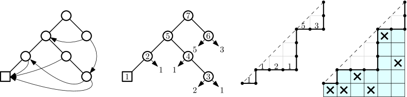
Horizontally decorated Dyck paths can also be interpreted as classical Dyck paths, where below every horizontal step a box given by a unit square between the horizontal step and the line is marked, see Figure 3. This gives an interpretation connecting these paths with the heights of Dyck paths, which we will exploit later. Independently, Callan gave in [6] a more general bijection in which he called the paths column-marked subdiagonal paths, and Bassino and Nicaud studied in [3] a variation when counting some automata, where the paths stay above the diagonal, which they called -Dyck boxed diagrams.
Theorem 2.5.
There exists a bijection between relaxed binary trees of size and the set of horizontally decorated Dyck paths of length .
Proof.
Let be a relaxed binary tree of size , and its spine. For convenience, we identify the internal nodes in and , and pointers in with leaves (not the left-most one) in .
We now give a recursive procedure transforming into a horizontally decorated Dyck path . First, we take and label its internal nodes and the left-most leaf in postorder from to . Next, we define the following function that transforms into a lattice path in and . Given a binary tree , it either consists of two sub-trees , or it is a leaf . We thus define recursively by
It is clear that starts with for the left-most leaf. Let be with its starting removed. Note that performs a postorder traversal on where leaves are matched with and internal nodes with . Then, ends at and stays always strictly below because every binary (sub-)tree has one more leaf than internal nodes, and each initial segment of corresponds to a collection of subtrees of . Hence, is a Dyck path. Observe that the -th step in corresponds to the -st node in postorder, as the left-most leaf is labeled . Finally, for each step in , we label it by the label of the internal node (or the left-most leaf) to which its corresponding leaf in points in . We thus obtain a Dyck path with labels on the horizontal steps, and we define .
We have seen that the Dyck path is in bijection with the spine . To see that the labeling condition on horizontally decorated Dyck paths is equivalent to the condition on relaxed binary trees, we take a pointer pointing to a node with label that corresponds to a step with a certain coordinate . By construction of the Dyck path, comes after in postorder if and only if the step from comes after the step from , which is equivalent to , as the node with label is the left-most leaf and is not recorded as a step . We thus have the equivalence of the two conditions, so is indeed a bijection as claimed. ∎
The following result gives the claimed algorithm with quadratic arithmetic complexity to count such paths, which can also be used as a precomputation step of an algorithm that randomly generates these paths using a linear number of arithmetic operations for each path. These algorithms are also applicable to relaxed binary trees via the bijection .
Proposition 2.6.
Let be the number of horizontally decorated paths ending at . Then,
| for | |||||
| for | |||||
| for |
The number of relaxed binary trees of size is equal to .
Proof.
Let us start with the boundary conditions. First of all, no such path is allowed to cross the diagonal , thus for . Second, the paths consisting only of horizontal steps stay at altitude and admit therefore just one possible label for each step, i.e., for .
For the recursion we consider how a path can jump to . It either uses a step from or it uses a step from . In the second case, there are possible decorations as the path is currently at altitude . ∎
Remark 2.7 (Compacted trees of bounded right height).
This restriction naturally translates relaxed binary trees of right height at most from [17] into horizontally decorated Dyck paths of height at most , where height is the maximal normal distance rescaled by from a lattice point on the path to the diagonal. In other words, these paths are constrained to remain between the diagonal and a line translated to the right parallel to the diagonal by unit steps.
2.2 Compacted binary trees
Given a relaxed tree , an internal node is called a cherry if its children in the spine are both leaves and none of them is the left-most one. According to the discussion at the end of Section 4 in [17], the only obstacle for a relaxed tree to be a compacted tree is a cherry with badly chosen pointers. For the convenience of the reader, we now recall and formalize this observation in the following proposition.
Proposition 2.8.
A relaxed tree is a compacted tree if and only if there are no two nodes in which share the same left child and the same right child . Moreover, if is not a compacted tree, such a pair exists where is a cherry and precedes in postorder.
Proof.
The “only if” part follows directly from Definition 2.2. We now focus on the “if” part. Suppose that is not a compacted tree, which means there is at least a pair of internal nodes such that precedes and , with defined in Definition 2.2. Now we want to show that there is one such pair with being a cherry. We take such a pair . If is a cherry, the claim holds. Otherwise, without loss of generality, we suppose that the left child of is not a leaf. Let be the left child of . If is an internal node, we take . Otherwise, we take to be the internal node pointed to by . By definition, we have , and clearly precedes in postorder. We thus obtain a new pair with the same conditions but of greater depth in the spine. However, since the spine has finite depth, this process cannot continue forever. As it only stops when is a cherry, we have the existence of such a pair with a cherry. ∎
The restriction described in Proposition 2.8 has an analogue in the class of horizontally decorated paths: We label every step with its final altitude plus one, which corresponds to its row number in the interpretation with marked boxes, and which also corresponds to the traversal/process order in postorder of its internal node in the relaxed tree; compare Figure 3. Recall that each step is already labeled. For any step , let be its label. We associate to every step a pair of integers , which correspond to the labels of its left and right children. First, let be the step before and set . Next, draw a line from the ending point of in the southwest direction parallel to the diagonal, and stop upon touching the path again. Let be the last step before that ends on this line (if there is no such step, set ). Then set .
Definition 2.9.
A C-decorated path is a horizontally decorated path where the decorations and of each pattern of consecutive steps fulfill for all preceding steps .
Proposition 2.10.
The map bijectively sends the set of compacted trees of size to the set of C-decorated Dyck paths of length .
Proof.
Recall from Theorem 2.5 that the map is a bijection sending relaxed trees of size to the set of horizontally decorated Dyck paths of size . C-decorated paths are defined precisely so that their corresponding relaxed trees satisfy the condition of Proposition 2.8. Therefore, forms a bijection between C-decorated paths and compacted trees. ∎
The key observation for the counting result is that exactly one pair of labels is avoided for each preceding step of a consecutive pattern . Applying this classification to the previous result we get a similar quadratic-time recurrence for compacted binary trees.
Proposition 2.11.
Let be the number of C-decorated paths ending at . Then,
| for | |||||
| for | |||||
| for |
The number of compacted binary trees of size is equal to .
Proof.
In the first case, the term counts the paths ending with a -step while counts the paths ending with a -step. The term occurs because, for each C-decorated path ending at , there are exactly paths formed by adding an additional that are not C-decorated paths. ∎
Note that one might also count the following simpler class which is in bijection with C-decorated paths, albeit without a natural bijection.
Definition 2.12.
A H-decorated path is a horizontally decorated path where the decorations and of each pattern of consecutive steps fulfill except for .
In terms of marked boxes, this constraint translates to the fact that, below the horizontal steps in each consecutive pattern , the marks must be in different rows except possibly for the lowest one.
3 Heuristic analysis
In this section, we will explain briefly some heuristics and an ansatz that we will apply later to get the asymptotic behavior of and . These heuristics are closely related to the asymptotic behavior of Dyck paths and the Airy function.
3.1 An intuitive explanation of the stretched exponential
We can consider as a weighted sum of Dyck paths, where each Dyck path has a weight that is the number of horizontally decorated Dyck paths that it gives rise to. There is thus a balance of the number of total paths and their weights for the weighted sum . On the one hand, most paths have an (average) height of (i.e., mean distance to the diagonal). On the other hand, their weight is maximal if their height is , i.e., they are close to the diagonal. In other words, typical Dyck paths are numerous but with small weight, and Dyck paths atypically close to the diagonal are few but with enormous weight. The asymptotic behavior of the weighted sum of Dyck paths that we consider should be a result of a compromise between these two forces. We will now make this more explicit by analyzing Dyck paths with height approximately for some .
Given a Dyck path with steps and as in Definition 2.3, let be the -coordinate of the -th step . The number of Dyck paths with bounded uniformly satisfy the following property.
Proposition 3.1 ([22, Theorem 3.3]).
For a Dyck path of length chosen uniformly at random, let be the -coordinate of the -th step . For , we have
Let the number of horizontally decorated Dyck paths whose unlabeled version is the Dyck path . For a randomly chosen Dyck path of length with bounded uniformly by , we heuristically expect most values of to be of the order , with of order . This leads to the following approximation:
Here, is some constant depending on . This approximation is only heuristically justified and very hard to prove. The contribution of Dyck paths with uniformly bounded by should thus roughly be , with and a constant depending on . Here, comes from the growth constant of Dyck paths. The function is minimal at , which maximizes the contribution, leading to the following heuristic guess that the number of relaxed binary trees should satisfy
for some constant . Furthermore, we anticipate that the main contribution should come from horizontally decorated Dyck paths with mostly of order . Since most such ’s should be of order , we can even state the condition above as for most endpoints of horizontal steps. This heuristic is the starting point of our analysis.
3.2 Weighted Dyck meanders
The heuristics of the previous section suggest that the mean distance to the diagonal will play an important role. Therefore, we propose another model of lattice paths emphasizing this distance. A Dyck meander (or simply a meander) is a lattice path consisting of up steps and down steps while never falling below . It is clear that Dyck paths of length are in bijection with Dyck meanders of length ending on with the transcription . This bijection can also be viewed geometrically as the linear transformation . This transformation will simplify the following analysis. We can consider Dyck meanders as initial segments of Dyck paths.
Furthermore, we have seen that a rescaling by seems practical. So we consider the following weight on steps in a meander . If starts from , then its weight is , and the weight of is the product of the weights of its steps . Let denote the weighted sum of meanders ending at . We get the following recurrence for .
Proposition 3.2.
The weighted sum defined above for meanders ending at satisfies the recurrence
| (6) |
Proof.
We concentrate on the first case, as the boundary cases follow directly from the definition of meanders. Given a meander ending at with , the last step may be an up step or a down step. The contribution of the former case is , with the weight of the last up step taken into account. The contribution of the latter case is simply . We thus get the claimed recurrence. ∎
Corollary 3.3.
For integers of the same parity, we have
When are not of the same parity, we have .
In particular, the number of relaxed trees of size is given by .
Proof.
For some simple cases of , elementary computations show that for , , and .
3.3 Analytic approximation of weighted Dyck meanders
The heuristic in Section 3.1 suggests that the main weight of comes from the region . It thus suggests an approximation of of the form
| (7) |
for some functions and , where we expect for some . The idea is that describes how the total weight for a fixed grows, and describes the rescaled weight distribution in the main region .
Let be the ratio . Suppose that , the recurrence relation becomes
| (8) |
Now, since we expect , we postulate that the ratio behaves like
| (9) |
and that is analytic. Using these assumptions, we can expand (8) as a Puiseux series in . Moving all terms to the right-hand side yields
Solving the differential equation under the condition when yields the unique solution (up to multiplication by a constant)
| (10) |
The condition on the behavior of near is motivated by the experimental observation that is quickly decaying for close to . We also insist that as , which implies that where is the first root of the Airy function , i.e. the largest one as all roots are on the real negative axis; see [1, p. 450]. Now, using this conjectural value of , it follows that (ignoring polynomial terms)
This suggests that the number of relaxed trees behaves like
which is compatible with what we want to prove.
We observe that (8) can be expanded into a Puiseux series of by taking appropriate series expansions of and . Therefore, to refine the analysis above, it is natural to look at the expansion of in (9) to more subdominant terms, and to postulate a more refined ansatz of than (7), probably as a series in . Indeed, if we take
and
then using the same method we can reach the polynomial part of the asymptotic behavior of as
In general, we can postulate
and
The proof of our main result on relaxed binary trees is based on choosing the cutoff appropriately, and using perturbations of that truncation to bound .
3.4 Discussion on the constants
One of the first steps in our method involves taking ratios (or equivalently ) of successive terms. From the leading asymptotic behavior of these ratios we can deduce the exact asymptotic form up to the constant term. Unfortunately, however, this method makes it impossible to exactly determine the constant term . In this section we give estimates of the constant terms: we believe that there are constants and such that
Based on the analysis in Section 3.3, we expect the ratios to behave like
for any positive integer , with the sequence beginning with the terms . This is equivalent to the existence of a sequence such that behaves like
for any positive integer . In this equation, is the constant term that we aim to approximate. A simple way to approximate is to write
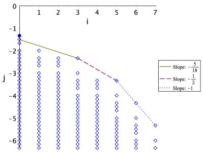
Then the graph of the values of plotted against (because is close to ) should be roughly linear (see Figure 4(a)), and the point where it crosses the -axis can be taken as an approximation for . This yields . We get a more precise estimate as follows: Fix to be some positive integer. Then, for each , consider the integers . For each such we expect the equation
to be approximately true. We then solve this system of equations for as though the equations were exact, using known, exact values of . This yields approximations for . Denote the approximation thus obtained for by . Note that this is equivalent to writing as a weighted sum of the numbers , which cancels the terms for . For example, if then . Hence, if our assumptions are correct then . Taking and plotting against (because is close to ) as in Figure 4(b) yields the approximation , where we expect the quoted digits to be correct. In Figures 4(c) and 4(d) we show a similar analysis of the counting sequence for compacted trees, yielding the approximation .
4 Proof of stretched exponential for relaxed trees
In this section we prove upper and lower bounds for the number of relaxed trees. These bounds differ only in the constant term, so they completely determine both the stretched exponential factor and the polynomial factor in the asymptotic number of relaxed trees for large .
Recall from Corollary 3.3 that the number of relaxed trees of size is given by , where the terms are given by the recurrence relation (6) which we repeat here for the convenience of the reader:
Our proofs of the upper and lower bounds for relaxed trees come from more general bounds for the numbers , which we prove by induction. Suppose that and are sequences of non-negative real numbers satisfying
| (11) |
for all sufficiently large and all integers . We define the sequence by and . By induction on , for some constant , the following inequality holds for all sufficiently large and all :
| (12) | ||||
Here (IS) marks the “Induction Step”. Similarly, if we can show the opposite of (11), it will imply that
for all sufficiently large and all integers .
Comparing to the heuristic analysis in Section 3.3, we see that acts as the function , and as . Therefore, we should expect to be close to (10), and to be a slight deviation of (9).
In Lemma 4.2 we will prove that certain explicit sequences and satisfy (11), which will lead to a lower bound on the numbers . Similarly, in Lemma 4.4 we will show that other explicit sequences and satisfy the opposite of (11), which therefore yields an upper bound on the numbers . Together, these two bounds determine the exact asymptotic form of the numbers up to the constant term.
In order to prove these bounds with the explicit expressions of and , we will consider the difference between the right- and the left-hand side of (11). Then we will show that this difference is non-negative. We start by expanding the involved Airy function and its derivative in the neighborhood of an appropriate point , leading to a sum of the form
where and can be expressed as Puiseux series in whose coefficients are fractional polynomials in . By looking at the “Newton polygon” of these Puiseux series, we can pick out the dominant term at different regimes of and , leading to a proof of (11) (or the reverse direction).
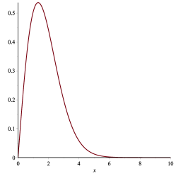
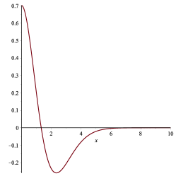
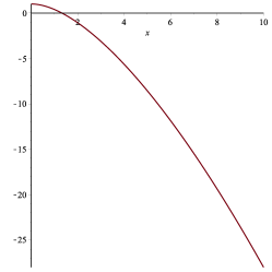
The following Lemma summarizes some elementary results on the relation between the Airy function Ai and its derivative . We will use these results in Lemmas 4.2 and 4.4 to bound the subsequently defined auxiliary sequence .
Lemma 4.1.
The functions
| and |
are infinitely differentiable and monotonically decreasing on with .
Proof.
First, by l’Hospital’s rule it is easy to see that . Second, as is the largest root of , the functions and are infinitely differentiable as compositions of differentiable functions. It remains to prove the monotonicity; see Figure 5. A local expansion at shows that the functions are initially decreasing. The same holds for large due to the approximation , see [1, Equation 10.5.49], giving
| (13) |
for . We will show that and are always negative for . Note that and will change sign only once at .
We present the following argument for the monotonicity of . Assume that there exists an such that . Then, as is initially and finally decreasing, there must exist such that and .
The second derivatives are equal to
These lead to , thus also the contradiction . The argument for the monotonicity of is analogous, except that the second derivative is now
leading to the contradiction . ∎
Later we will use the value which is the unique root of and to determine the dominant term in the expansion of our series in and .
4.1 Lower bound
Lemma 4.2.
For all let
Then, for any , there exists an such that
| (14) |
for all and for all .
Proof.
First, define the following sequence
where
with . Then the inequality (14) is equivalent to with , , , , and as well as , , and . Next, we expand in a neighborhood of
| (15) |
and we get the following expansion
where and are functions of and and may be expanded as power series in with coefficients polynomial in . As long as and , this series converges absolutely because the Airy function is entire and so all functions expanded are analytic in the region defined by and .
As a first step we compute the possible range of the powers in and . We will start by showing that for , . The expansions of the three involved Airy functions only give terms of the form , with . Due to the differential equation , the term takes the form . Hence, all terms in the expansion of the Airy function are of the form or for some . Due to the factor in the definition of , this implies that for . Additionally, it also implies that the coefficients of are equal to for .
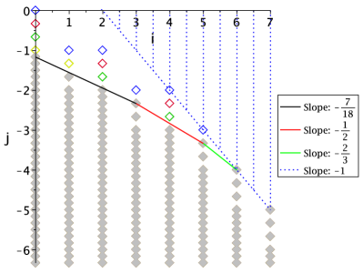
Next, we strengthen this result by choosing suitable values for in the definition of in order to eliminate more initial coefficients. Then, we will show that the remaining terms satisfy . We performed this tedious task in Maple and we refer to the accompanying worksheet [27] for more details. The results are summarized in Figure 6 where the initial non-zero coefficients are shown. A diamond at is drawn if and only if the coefficient is non-zero. It is an empty diamond if the given choice of and makes it disappear, whereas it is a solid diamond if it remains non-zero. The convex hull is formed by the following three lines
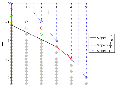

Next, we distinguish between the contributions arising from and . The expansions for tending to infinity start as follows, where the elements on the convex hull are written in color:
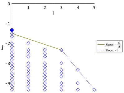
We now choose which leads to a positive term and set to eliminate the term of order from the convex hull (it is replaced by ). Then, the non-zero coefficients are shown in Figure 7. Next, for fixed (large) we prove that for all the dominant contributions in are positive. Therefore, we consider three different regimes. Let be the unique positive root of from Lemma 4.1.
-
1.
Consider the range of small values of given by . In this range and are both positive. Moreover, the (red) coefficients of are dominated by for large , while the (blue) coefficients of apart from the term are dominated by . By Lemma 4.1 we have
Hence, , and it can therefore be treated as if it belonged to the coefficients of . Thus, as the dominating terms are positive, there exists some such that whenever and .
-
2.
Next, consider the central range . Here, we have . On the one hand, as seen in the left part of Figure 7, the (red) coefficients of are still dominated by (which holds up to ). On the other hand, in this range the term dominates all other (blue) coefficients of (due to ). Since in this range, this implies that there exists some (sufficiently large) such that whenever and .
-
3.
Finally, consider the range of large values . By the reasoning on in Lemma 4.1 we see that . Therefore, the (blue) term dominates all of the (red) terms of as well as all other (blue) terms of . Hence there exists some such that whenever and .
Choosing completes the proof. ∎
Remark 4.3.
Now, to complete the lower bound we define the sequence , i.e.,
Then, in the first case we get the following inequality for all sufficiently large
using Lemma 4.2 with . Note that we could choose any , as we just need for large . In the second case we have
Finally, we write and we deduce by induction that for some constant , all sufficiently large and all . In particular, it follows from (12) that the number of relaxed trees of size is bounded below by
| (16) |
for some constant . In the next section we will show an upper bound with the same asymptotic form, but with a different constant .
4.2 Upper bound
Next, we consider a similar auxiliary sequence which will give rise to an upper bound on the number of relaxed binary trees.
Lemma 4.4.
Choose fixed and for all let
Then, for any , there exists a constant such that
| (17) |
for all and all .
Proof.
The proof follows the same lines as that of Lemma 4.2. Therefore we only focus on the needed modifications. As a first step we define the following sequence
Then the inequality (17) is equivalent to . Again, we expand in a neighborhood of and we get (see [27] for more details)
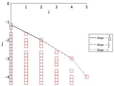
where and are functions of and and may again be expanded as power series in with coefficients polynomial in . Now, it is easy to see that for , where the shift by compared to the lower bound is due to the factor . The initial non-zero coefficients are shown in Figure 8. The four lines (black, red, green, blue) of the convex hull are
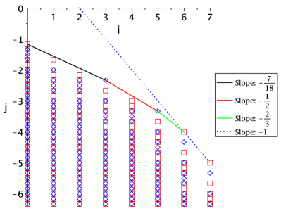

Next, we distinguish between the contributions arising from and . The non-zero coefficients are shown in Figure 9. The expansions for tending to infinity start as follows, where the elements on the convex hull are written in color.
Let be again the unique positive root of from Lemma 4.1. In order to prove that for , we consider the following four regions:
-
1.
,
-
2.
,
-
3.
,
-
4.
.
Recall that in the proof that in Lemma 4.2, we considered almost the same first regions, except that in that case the upper bound on the third region was slightly larger (). So the main difference here is the addition of the fourth region, which is required for this lemma to apply up to .
The treatments of the first regions are analogous to those in Lemma 4.2 except for 2 minor changes. First, in the second and third regime we include the additional variable to make the dominant term positive. Second, in the third regime an additional dominant term appears for which is positive anyway.
Finally, in the fourth regime, the aforementioned term is positive and dominates all other blue terms. However, the dominant red term is , which is negative, so it suffices to show that this is dominated by the blue term. Indeed, due to (13) we know that as tends to infinity, . Hence, the blue term dominates in this entire region . ∎
To finish the proof of the upper bound, we will choose some constant and define a sequence by the same rules as except that whenever and . Then, writing , we can use the lemma above to show by induction that the numbers satisfy the inequality.
for some constant and all sufficiently large ; compare (12). In particular, the numbers are bounded above by
for some constant . The rest of this section is dedicated to proving that there is some choice of such that for all .
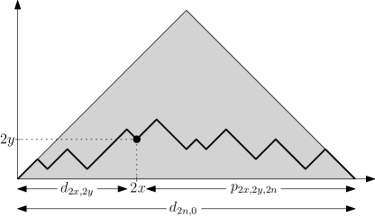
In order to finish our proof of the upper bound for the numbers , we will use the interpretation of these numbers as weighted Dyck paths, described in Section 3.2. It will be useful to have an upper bound on the number of these paths which pass through a certain point as a proportion of the total weighted number of paths. Let denote the weighted number of paths from to ; see Figure 10. Then the proportion of the weighted Dyck paths that pass through is
The following lemma yields an upper bound on the number .
Lemma 4.5.
The numbers satisfy the inequality
for integers satisfying .
Proof.
First we note that the numbers are determined by the recurrence relation
along with the initial conditions and . We will now prove the statement of the lemma by reverse induction on . Our base case is , for which the inequality clearly holds. For the inductive step, we assume that the inequality holds for and all , and we will prove that it holds for . It suffices to prove that for the following inequality holds
Let denote the left-hand side of this inequality. Using the recurrence relation, we can rewrite as
Now, by the inductive assumption we get the inequalities and , where the latter even holds for as then both sides are . It follows that
as desired. This completes the induction, which proves the inequality for . We refer to the accompanying worksheet [27] for more details. ∎
In particular, it follows from this lemma that
Moreover, note that the proportion of weighted paths passing through satisfies . Hence, the proportion satisfies
| (18) |
From the lower bound (16) we have
so we now desire an upper bound for . It will suffice to use the upper bound
which holds because the right-hand side is the number of (unweighted) paths from to , and all weights on our weighted paths are smaller than . We are now ready to prove the following lemma
Lemma 4.6.
For all there exists a constant with the following property: Recall that is the weighted number of paths ending at . Let be the number of these paths such that no intermediate point on the path satisfies and . Then for all .
Proof.
We can rewrite the desired inequality as
Note that the left-hand side is equal to the proportion of weighted paths with at least one intermediate point satisfying and . The proportion of weighted paths which go through any such point is bounded above by
The right-hand side of this inequality behaves like
| (19) |
for large . Hence, there is some constant such that
for all satisfying . Now, the proportion of weighted paths passing through at least one point is no greater than the sum of the proportions of paths going through each such point. Hence
The sum on the right converges to a value less than for sufficiently large . This completes the proof of the lemma. ∎
Remark 4.7.
Choosing instead of one can show that (19) behaves like . Hence, any gives the same result, yet is not sufficient.
Finally, we define as in Lemma 4.6 with some fixed . Then it follows from Lemma 4.4 that there is some constant such that
for all . Hence
completing the proof of the upper bound. We have now proven upper and lower bounds for the number of relaxed trees, which differ only in the constant term. Therefore,
5 Proof of stretched exponential for compacted trees
We will now deal with compacted binary trees, whose recurrence as in Proposition 2.11 has negative terms. We start by transforming the terms counting compacted trees to a sequence using the equation
for even. Then, the terms are determined by the recurrence
and the number of compacted trees of size is equal to .
The method that we applied to (6) in the relaxed case does not directly apply to this recurrence, as there is a negative term on the right-hand side. We solve this problem using the following lemma:
Lemma 5.1.
For and , the term for compacted binary trees is bounded below by
and bounded above by
That is, . Furthermore, where is defined by the same expression as but with each replaced by .
Proof.
We start with the upper bound of . In order to prove that, we will compute successively stronger upper bounds. We start with the trivial upper bound
| (20) |
Applying this bound to then we find that
| (21) |
Adding times this inequality to the defining equation of yields
Now we will prove that . Note that the first two inequalities (20) and (21) in this proof become equalities when each is replaced by . Adding times the latter (now) equality (21) to the defining equation (6) of yields
We then see that through induction on .
For the lower bound on , we start with the inequality
| (22) |
This is clear for , and for it is an equality. We can then deduce this inequality (22) for all using induction: Assume that the statement is true for all and all . Then, for and , we have
Hence,
This completes the induction. Moreover, it shows that
| (23) |
for . It is easy to see that this stronger inequality (23) also holds for and . Applying (23) to then yields
Finally, combining this with the inequality
yields the desired result.∎
The advantage of the bounds in the lemma above is that all terms are positive, so we can derive the asymptotics using the same techniques as for relaxed binary trees. Note that the behavior stays the same in the process of deriving the Newton polygons and leads to the same pictures as shown in Figures 6 and 7.
5.1 Lower bound
The following result is analogous to Lemma 4.2.
Lemma 5.2.
For all let
Then, for any , there exists a constant such that
for all and all .
Proof.
The proof is analogous to the case of relaxed trees. In this case, the expansions for start as follows, where the elements on the convex hull are written in color:
In this expansion we choose , which leads to a positive term , and we also choose (instead of in the relaxed trees case), which kills the leading coefficient of for small . Then, the behavior and thus the pictures are identical to the case of relaxed trees shown in Figures 6 and 7. Hence, the proof follows exactly the same lines as that Lemma 4.2. ∎
As in the relaxed case, we define a sequence , i.e.,
Then defining , we get by induction
for some . In particular, it follows that the number of compacted trees of size is bounded below by
| (24) |
for some constant . In the next section we will show an upper bound with the same asymptotic form, but with a different constant .
5.2 Upper bound
The following result is analogous to Lemma 4.4.
Lemma 5.3.
Choose fixed and for all let
Then, for any , there exists a constant such that
for all and all .
Proof.
The proof is again analogous to the case of relaxed trees. In this case, the expansions for start as follows, where the elements on the convex hull are written in color:
In this expansion we choose , which leads to a positive term , and again . Then, the behavior and therefore the pictures are identical to the case of relaxed trees shown in the Figures 8 and 9; see the proof of Lemma 4.4 for more details. ∎
As in the relaxed tree case, the inequality of Lemma 5.3 is only proven for , so we need to do more work to handle the case and deduce the desired upper bound. In order to use the lemma, we define a new sequence by the recurrence relation
Then it follows from Lemma 5.1 that for all , as share the same recurrence as in Lemma 5.1. Now consider some large , to be determined later, and define a second sequence by the same rules as except that whenever and . Then, using Lemma 5.3 and defining , we can show by induction that there is some constant such that
It follows that there is some constant such that
Hence, it suffices to prove that there is some choice of and some constant such that for all . Therefore, we first define a class of weighted paths with the step set and weights corresponding to the recurrence defining . Then is the weighted number of paths from to . We start with the following lemma, which is analogous to Lemma 4.5.
Lemma 5.4.
Let denote the weighted number of paths from to . Then the numbers satisfy the inequality
for integers satisfying and .
Proof.
The proof is along the same lines as the proof of Lemma 4.5. As in that case, it suffices to prove that
| (25) |
for all . We proceed by reverse induction on , with base case . For the inductive step, note that satisfies the following recurrence for :
Now in order to prove (25), we expand the left-hand side using the recurrence relation above. For , we use the inductive assumption, which says that (25) holds for all larger values of and all , to show that
for some explicit rational functions , and . Due to the nature of the functions , and , we can prove that the right-hand side above is positive using the inequalities
which follow directly from the recurrence relation. The case is similar, though we instead find
and we prove that the right hand side is positive using the inequalities
which follow directly from the recurrence relation. We refer the accompanying worksheet [27] for more details. ∎
Now, among the weighted paths starting at and ending at , the proportion of those passing through some point is
We used the fact that which we proved inductively using Lemma 5.1, and we also used the lower bound (24) for . We can finish in exactly the same way as in Lemma 4.6 for relaxed trees, thereby showing that there is some choice for such that for all .
Recall that and there is some constant such that This implies that
The right-hand side behaves asymptotically like , hence there is some constant such that
for all . This completes the upper bound. Indeed, since we have now proven both the upper and lower bounds, which differ only in the constant term, they imply that
6 Minimal finite automata
In this section we use the results on compacted and relaxed trees to give bounds on the enumeration of a certain class of deterministic finite automata considered in [12, 23, 11]. We start with some basic definitions of automata.
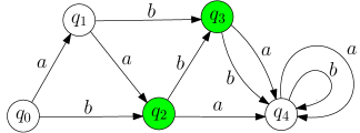
A deterministic finite automaton (DFA) is a -tuple , where is a finite set of letters called the alphabet, is a finite set of states, is the transition function, is the initial state, and is the set of final states (sometimes called accept states). A DFA can be represented by a directed graph with one vertex for each state , with the vertices corresponding to final states being highlighted, and for every transition , there is an edge from to labeled (see Figure 11).
A word is accepted by if the sequence of states defined by and for ends with a final state. The set of words accepted by is called the language recognized by . It is well-known that DFAs recognize exactly the set of regular languages. Note that every DFA recognizes a unique language, but a language can be recognized by several different DFAs. A DFA is called minimal if no DFA with fewer states recognizes the same language. The Myhill-Nerode Theorem states that every regular language is recognized by a unique minimal DFA (up to isomorphism) [19, Theorem 3.10]. For more details on automata see [19].
Since every regular language defines a unique minimal automaton, one can define the complexity of the language to be the number of states in the corresponding automaton. More precisely, this is an interpretation for the space complexity of the language.
The asymptotic proportion of minimal DFAs in the class of (not necessarily acyclic) automata was solved by Bassino, Nicaud, and Sportiello in [2], building on enumeration results by Korshunov [21, 20] and Bassino and Nicaud [3]. This result also exploits an underlying tree structure of the automata, but this tree structure comes from a different traversal than what we use. In that case, no stretched exponential appears in the asymptotic enumeration, and the minimal automata account for a constant fraction of all automata.
The analogous problem in the restricted case of automata that recognize a finite language is widely open (see for example [11]). This corresponds to counting finite languages by their space complexity. To show the relation between these automata and compacted and relaxed trees, we need the following lemma from [23, Lemma 2.3] or [19, Section 3.4]. For the convenience of the reader, we include a proof of one direction here.
Lemma 6.1.
A DFA is the minimal automaton for some finite language if and only if it has the following properties:
-
•
There is a unique sink . That is, a state which is not a final state and with all transitions from end at that is, .
-
•
is acyclic: the corresponding directed graph has no cycles except for the loops at the dead state.
-
•
is initially connected: for any state there exists a word such that reaches the state upon reading .
-
•
is reduced: for any two different states , , the two automata with initial state and recognize different languages.
Proof.
We will show one direction of this proof: that a minimal automaton has the four properties. For a proof of the reverse direction see e.g. [23, Lemma 2.3] or [19, Section 3.4].
If is minimal but not reduced then there are two states and from which the same language is recognized. These two states can be merged into a single state without changing the language, contradicting the minimality of . This implies that there is at most one state from which the empty language is recognized. Moreover, such a state must exist for the language to be finite. This state must therefore be the unique sink.
The fact the is acyclic follows immediately from the fact that recognizes a finite language. Finally, if we remove from all states that cannot be reached, the language accepted by the automaton will not be changed, so by the minimality of , there must be no such states and must be initially connected. ∎
We note here one consequence of this lemma: since the automaton is acyclic, there must be some state other than the sink such that all transitions from end at . Then since the automaton is reduced, there must be only one such state , and it must be an accept state.
Now using our asymptotic results on compacted and relaxed trees, we give the following new bounds on the asymptotic number of such automata, determining their asymptotics up to a polynomial multiplicative term.
Theorem 6.2.
Let be the number of minimal DFAs over a binary alphabet with transient states (and a unique sink) that recognize a finite language. Then,
As a consequence, there exist positive constants and such that
Proof.
By the lemma above, a compacted tree can be transformed into an automaton that recognizes a finite language over the alphabet as follows: The states of the automaton correspond to the internal nodes and the leaf of . The initial state corresponds to the root, and at each state, the transition after reading (resp. ) is given by the left (resp. right) child or pointer in . The leaf is designated as the unique sink, and we can choose any subset of internal nodes as final states, with the condition that the unique node with two pointers to the sink is always a final state.
To prove the minimality of such automata, we just need to check the four conditions of Lemma 6.1. The fact that is acyclic and has a unique sink follow immediately from the fact the is a DAG. Then is initially connected because has a unique source. Now we will show that is reduced. For any state in , let denote the language recognized by the automaton with initial state . Now suppose that is not reduced and let and be different states of satisfying . We also assume that amongst all such pairs , the length of the longest word in is minimized. Since the unique node with both pointers to the sink is a final state, the language can only be empty if and are both the final state, which is impossible. Since we must have and . Then, the minimality condition on the language implies that and . But this means that the node and in corresponding to and have the same left child and the same right child, contradicting the fact that is compacted. This completes the proof that is reduced.
Hence, each of the subsets of the remaining states (not the sink and not the node with two pointers to the sink) gives a valid minimal automaton of size .
Applying the same construction to relaxed trees gives an upper bound, as every minimal automaton, after forgetting which states are final, corresponds by construction to a relaxed tree. Note that this observation has already been made in [23, Equation (1)], yet the asymptotics was not known. ∎
Using the methods of the present work, the authors showed in a companion paper [13] that
To our knowledge, our results give the best known bounds on the asymptotic number of minimal DFAs on a binary alphabet recognizing a finite language. Note that they disprove the conjecture for some of Liskovets based on numerical data; see [23, Equation (16)]. Previously, Domaratzki derived in [10] the lower bound
with , which implies the asymptotic bound (note that in his results). Furthermore, Domaratzki showed in [9] the upper bound
where are the Genocchi numbers defined by . This gives the asymptotic bound This bound, however, is much larger than the superexponential growth given by in our upper bound. While not explicitly formulated in the literature, it is possible to bound the acyclic DFAs by general DFAs using the results by Korshunov [21, 20] (see also [3, Theorem 18]). Thereby, we get the upper bound
where with being the solution of , and therefore , which is significantly larger than the exponential growth in our upper bound.
Acknowledgments
We would like to thank Tony Guttmann for sending us calculations on the asymptotic form of pushed Dyck paths. More generally, we thank him, Cyril Banderier and Andrea Sportiello for interesting discussions on the presence of a stretched exponential. We want to thank the anonymous referees for their detailed comments which improved the presentation of this work.
References
- [1] M. Abramowitz and I. A. Stegun. Handbook of Mathematical Functions With Formulas, Graphs, and Mathematical Tables, volume 55 of National Bureau of Standards Applied Mathematics Series. For sale by the Superintendent of Documents, U.S. Government Printing Office, Washington, D.C., 1964.
- [2] F. Bassino, J. David, and A. Sportiello. Asymptotic enumeration of minimal automata. In 29th International Symposium on Theoretical Aspects of Computer Science, volume 14 of LIPIcs. Leibniz Int. Proc. Inform., pages 88–99. Schloss Dagstuhl. Leibniz-Zent. Inform., Wadern, 2012.
- [3] F. Bassino and C. Nicaud. Enumeration and random generation of accessible automata. Theoret. Comput. Sci., 381(1-3):86–104, 2007.
- [4] N. R. Beaton, A. J. Guttmann, I. Jensen, and G. F. Lawler. Compressed self-avoiding walks, bridges and polygons. J. Phys. A, 48(45):454001, oct 2015.
- [5] M. Bousquet-Mélou, M. Lohrey, S. Maneth, and E. Noeth. XML compression via directed acyclic graphs. Theory Comput. Syst., 57(4):1322–1371, 2015.
- [6] D. Callan. A determinant of Stirling cycle numbers counts unlabeled acyclic single-source automata. Discrete Math. Theor. Comput. Sci., 10(2):77–86, 2008.
- [7] A. R. Conway and A. J. Guttmann. On 1324-avoiding permutations. Adv. in Appl. Math., 64:50–69, 2015.
- [8] A. R. Conway, A. J. Guttmann, and P. Zinn-Justin. 1324-avoiding permutations revisited. Adv. in Appl. Math., 96:312–333, 2018.
- [9] M. Domaratzki. Combinatorial interpretations of a generalization of the Genocchi numbers. J. Integer Seq., 7(3):Article 04.3.6, 11, 2004.
- [10] M. Domaratzki. Improved bounds on the number of automata accepting finite languages. Internat. J. Found. Comput. Sci., 15(1):143–161, 2004. Computing and Combinatorics Conference—COCOON’02.
- [11] M. Domaratzki. Enumeration of formal languages. Bull. Eur. Assoc. Theor. Comput. Sci. EATCS, 89:117–133, 2006.
- [12] M. Domaratzki, D. Kisman, and J. Shallit. On the number of distinct languages accepted by finite automata with states. J. Autom. Lang. Comb., 7(4):469–486, 2002.
- [13] A. Elvey Price, W. Fang, and M. Wallner. Asymptotics of Minimal Deterministic Finite Automata Recognizing a Finite Binary Language. In AofA 2020, volume 159 of LIPIcs, pages 11:1–11:13. Schloss Dagstuhl–Leibniz-Zentrum für Informatik, 2020.
- [14] A. Elvey Price and A. J. Guttmann. Numerical studies of Thompson’s group F and related groups. Internat. J. Algebra Comput., 29(2):179–243, 2019.
- [15] P. Flajolet and R. Sedgewick. Analytic combinatorics. Cambridge University Press, Cambridge, 2009.
- [16] P. Flajolet, P. Sipala, and J.-M. Steyaert. Analytic variations on the common subexpression problem. In Automata, languages and programming (Coventry, 1990), volume 443 of Lecture Notes in Comput. Sci., pages 220–234. Springer, New York, 1990.
- [17] A. Genitrini, B. Gittenberger, M. Kauers, and M. Wallner. Asymptotic enumeration of compacted binary trees of bounded right height. J. Combin. Theory Ser. A, 172:105177, 2020. arXiv:1703.10031.
- [18] A. J. Guttmann. Analysis of series expansions for non-algebraic singularities. J. Phys. A, 48(4):045209, 2015.
- [19] J. E. Hopcroft and J. D. Ullman. Introduction to automata theory, languages, and computation. Addison-Wesley Publishing Co., Reading, Mass., 1979. Addison-Wesley Series in Computer Science.
- [20] A. D. Korshunov. Enumeration of finite automata. Problemy Kibernet., 34:5–82, 1978. (In Russian).
- [21] A. D. Korshunov. On the number of nonisomorphic strongly connected finite automata. Elektron. Informationsverarb. Kybernet., 22(9):459–462, 1986.
- [22] T. Kousha. Asymptotic behavior and the moderate deviation principle for the maximum of a Dyck path. Statist. Probab. Lett., 82(2):340–347, 2012.
- [23] V. A. Liskovets. Exact enumeration of acyclic deterministic automata. Discrete Appl. Math., 154(3):537–551, 2006.
- [24] C. Pittet and L. Saloff-Coste. On random walks on wreath products. Ann. Probab., 30(2):948–977, 2002.
- [25] D. Revelle. Heat kernel asymptotics on the lamplighter group. Electron. Comm. Probab., 8:142–154, 2003.
- [26] M. Wallner. A bijection of plane increasing trees with relaxed binary trees of right height at most one. Theoret. Comput. Sci., 755:1–12, 2019.
- [27] M. Wallner. http://dmg.tuwien.ac.at/mwallner, 2020.
- [28] E. M. Wright. The coefficients of a certain power series. J. London Math. Soc., 7(4):256–262, 1932.
- [29] E. M. Wright. On the coefficients of power series having exponential singularities. J. London Math. Soc., 8(1):71–79, 1933.
- [30] E. M. Wright. On the coefficients of power series having exponential singularities. II. J. London Math. Soc., 24:304–309, 1949.
A. Elvey Price, Laboratoire Bordelais de Recherche en Informatique, UMR 5800, Université de Bordeaux, 351 Cours de la Libération, 33405 Talence Cedex, France
E-mail address: andrew.elvey@univ-tours.fr
W. Fang, Laboratoire d’Informatique Gaspard-Monge, UMR 8049, Université Gustave-Eiffel, CNRS, ESIEE Paris, 5 Boulevard Descartes, 77454 Marne-la-Vallée, France
E-mail address: wenjie.fang@u-pem.fr
Website: http://igm.univ-mlv.fr/~wfang/
M. Wallner, Laboratoire Bordelais de Recherche en Informatique, UMR 5800, Université de Bordeaux, 351 Cours de la Libération, 33405 Talence Cedex, France; Institute of Discrete Mathematics and Geometry, TU Wien, Wiedner Hauptraße 8–10, 1040 Wien, Austria
E-mail address: michael.wallner@tuwien.ac.at
Website: https://dmg.tuwien.ac.at/mwallner/