An extended charge-current formulation of the electromagnetic transmission problem

Abstract

A boundary integral equation formulation is presented for the electromagnetic transmission problem where an incident electromagnetic wave is scattered from a bounded dielectric object. The formulation provides unique solutions for all combinations of wavenumbers in the closed upper half-plane for which Maxwell’s equations have a unique solution. This includes the challenging combination of a real positive wavenumber in the outer region and an imaginary wavenumber inside the object. The formulation, or variants thereof, is particularly suitable for numerical field evaluations as confirmed by examples involving both smooth and non-smooth objects.

1 Introduction

This work is about transmission problems. A simply connected homogeneous isotropic object is located in a homogeneous isotropic exterior region. A time harmonic incident wave, generated in the exterior region, is scattered from the object. The aim is to evaluate the fields in the interior and exterior regions.

We present boundary integral equation (BIE) formulations for the solution of the scalar Helmholtz and the electromagnetic Maxwell transmission problems. We show that our integral equations have unique solutions for all wavenumbers $k_{1}$ of the exterior domain and $k_{2}$ of the object with $0\leq{\rm{Arg}}(k_{1}),{\rm{Arg}}(k_{2})<\pi$, and for which the partial differential equation (PDE) formulations of the two problems have unique solutions. As we understand it, there is no other BIE formulation of the electromagnetic problem known to the computational electromagnetics community that can guarantee unique solutions for the wavenumber combination

$${\rm{Arg}}(k_{1})=0\,,\quad{\rm{Arg}}(k_{2})=\pi/2\,,\quad\mbox{and}\quad k_{2}^{2}/k_{1}^{2}\neq-1\,.$$ (1)

We refer to the combination (1) as the plasmonic condition since it enables discrete quasi-electrostatic surface plasmons in smooth, infinitesimally small, objects [25], continuous spectra of quasi-electrostatic surface plasmons in non-smooth objects [12], and undamped surface plasmon waves along planar surfaces [23, Appendix I]. Wavenumbers with ${\rm{Arg}}(k_{1})=0$ and $\pi/4<{\rm{Arg}}(k_{2})\leq\pi/2$ are of special interest in the areas of nano-optics and metamaterials because in this range weakly damped surface plasmons in subwavelength objects and weakly damped dynamic surface plasmon waves in objects of any size can occur. These phenomena become increasingly pronounced, and useful in applications, as ${\rm{Arg}}(k_{2})$ approaches $\pi/2$ [14, 20]. It is important to have uniqueness under the plasmonic condition, despite that there are no known materials that satisfy this condition exactly, since non-uniqueness implies spurious resonances that deteriorate the accuracy of the numerical solution also for ${\rm{Arg}}(k_{1})=0$, $\pi/4<{\rm{Arg}}(k_{2})<\pi/2$.

It is relatively easy to find a BIE formulation of the scalar transmission problem since one has access to the fundamental solution to the scalar Helmholtz equation. It remains to make sure that the boundary conditions are satisfied and that the solution is unique. To find a BIE formulation of the electromagnetic transmission problem, based on the same fundamental solution, is harder. Apart from satisfying the boundary conditions and uniqueness one also has to make sure that the solution satisfies Maxwell’s equations. Otherwise the two problems are very similar.

Our BIE formulation of the scalar problem is a modification of the formulation in [16, Section 4.2]. While our formulation guarantees unique solutions under the plasmonic condition, provided that the object surface is smooth, the formulation in [16, Section 4.2] does not.

Our BIE formulation of the electromagnetic problem is a further development of the classic formulation by Müller, [22, Section 23]. In [21] it is shown that the Müller formulation has unique solutions for $0\leq{\rm{Arg}}(k_{1}),{\rm{Arg}}(k_{2})<\pi/2$, but as shown in [11], it may have spurious resonances under the plasmonic condition. The Müller formulation has four unknown scalar surface densities, related to the equivalent electric and magnetic surface current densities, and that leads to dense-mesh/low-frequency breakdown in field evaluations. Despite these shortcomings, the Müller formulation has been frequently used. Its advantages are emphasized in a recent paper [18] on scattering from axisymmetric objects where accurate solutions are obtained away from the low-frequency limit.

One way to overcome low-frequency breakdown in the Müller formulation is to increase the number of unknown densities from four to six by adding the equivalent electric and magnetic surface charge densities [9, 24, 27]. The charge densities can be introduced in two ways, leading to two types of formulations. The first type is decoupled charge-current formulations, where the charge densities are introduced after the BIE has been solved. The other type is coupled charge-current formulations, where the charge densities are present from the start. Unfortunately, both types of formulations can give rise to new complications such as spurious resonances and near-resonances. Several formulations in the literature ignore these complications, but in [27] a stable formulation is presented. In line with all other formulations in literature, uniqueness in [27] is not guaranteed under the plasmonic condition.

The main result of the present work is our extended charge-current BIE formulation of the electromagnetic transmission problem where two additional surface densities, related to electric and magnetic volume charge densities, are introduced. The formulation is given by the representation (64) and the system (65) below. The formulation is free from low-frequency breakdown and it provides unique solutions also under the plasmonic condition. Just like the Müller- and charge-current formulations it is a direct formulation, meaning that the surface densities are related to boundary limits of fields, or derivatives of fields. This is in contrast to indirect formulations [5, 6, 17, 27], where the surface densities lack immediate physical interpretation. Albeit somewhat more numerically expensive than competing formulations, our new formulation enables high achievable accuracy and since it is more robust this should outweigh the disadvantage of having eight densities. From a broader perspective one can say that our paper, and many other papers [9, 18, 21, 22, 24, 27], use integral representations of the electric and magnetic fields for modeling. It is also possible to start with representations of scalar and vector potentials and antipotentials [5, 6, 19].

The paper is organized as follows: Section 2 introduces notation and definitions common to the scalar and the electromagnetic problems. The scalar problem and two closely related homogeneous problems, to be used in a uniqueness proof, are defined in Section 3. Scalar integral representations containing two surface densities are introduced in Section 4. Section 5 proposes a system of BIEs for these densities. This system contains two free parameters and, as seen in Section 6, unique solutions are guaranteed by giving them proper values. Section 7 concerns the evaluation of near fields. The procedure for finding BIEs for the scalar problem is then adapted to the electromagnetic problem, defined along with two auxiliary homogeneous problems in Section 8. Integral representations of electric and magnetic fields in terms of eight scalar surface densities are given in Section 9 and a corresponding system of BIEs is proposed in Section 10. This BIE system contains four free parameters and again, as shown in Section 11, unique solutions are guaranteed by choosing them properly. Section 12 presents reduced two-dimensional (2D) versions of the electromagnetic BIE system whose purpose is to facilitate initial tests and comparisons. Section 13 reviews test domains and discretization techniques and Section 14 presents numerical examples, including what we believe is the first high-order accurate computation of a surface plasmon wave on a non-smooth three-dimensional (3D) object.

Appendix A presents boundary values of integral representations. Appendix B and C derive conditions for our representations of the electric and magnetic fields to satisfy Maxwell’s equations. In Appendix D a set of points $({\rm{Arg}}(k_{1}),{\rm{Arg}}(k_{2}))$ is identified for which the electromagnetic problem has at most one solution.

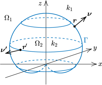
Figure 1: Geometry in $\mathbb{R}^{3}$. Inside $\Gamma$ the volume is $\Omega_{2}$ and the wavenumber $k_{2}$. Outside $\Gamma$ the volume is $\Omega_{1}$ and the wavenumber $k_{1}$. The outward unit normal is ${\boldsymbol{\nu}}$ at ${\boldsymbol{r}}$ and ${\boldsymbol{\nu}}^{\prime}$ at ${\boldsymbol{r}}^{\prime}$.

2 Notation

Let $\Omega_{2}$ be a bounded volume in $\mathbb{R}^{3}$ with a smooth closed surface $\Gamma$ and simply connected unbounded exterior $\Omega_{1}$. The outward unit normal at position ${\boldsymbol{r}}$ on $\Gamma$ is ${\boldsymbol{\nu}}$. We consider time-harmonic fields with time dependence $e^{-{\rm i}t}$, where the angular frequency is scaled to one. The relation between time-dependent fields $F({\boldsymbol{r}},t)$ and complex fields $F({\boldsymbol{r}})$ is

$$F({\boldsymbol{r}},t)=\Re{\rm e}\left\{F({\boldsymbol{r}})e^{-{\rm i}t}\right\}.$$ (2)

The volumes $\Omega_{1}$ and $\Omega_{2}$ are homogeneous with wavenumbers $k_{1}$ and $k_{2}$. See Figure 1, which depicts a non-smooth $\Gamma$ that is used later in numerical examples. An incident field is generated by a source somewhere in $\Omega_{1}$.

2.1 Layer potentials and boundary integral operators

The fundamental solution to the scalar Helmholtz equation is taken to be

$$\Phi_{k}({\boldsymbol{r}},{\boldsymbol{r}}^{\prime})=\frac{e^{{\rm i}k\lvert{\boldsymbol{r}}-{\boldsymbol{r}}^{\prime}\rvert}}{4\pi\lvert{\boldsymbol{r}}-{\boldsymbol{r}}^{\prime}\rvert}\,,\quad{\boldsymbol{r}},{\boldsymbol{r}}^{\prime}\in\mathbb{R}^{3}\,.$$ (3)

Two scalar layer potentials are defined in terms of a general surface density $\sigma$ as

$$\begin{split}S_{k}\sigma({\boldsymbol{r}})&=2\int_{\Gamma}\Phi_{k}({\boldsymbol{r}},{\boldsymbol{r}}^{\prime})\sigma({\boldsymbol{r}}^{\prime})\,{\rm d}\Gamma^{\prime}\,,\quad{\boldsymbol{r}}\in\Omega_{1}\cup\Omega_{2}\,,\\ K_{k}\sigma({\boldsymbol{r}})&=2\int_{\Gamma}(\partial_{\nu^{\prime}}\Phi_{k})({\boldsymbol{r}},{\boldsymbol{r}}^{\prime})\sigma({\boldsymbol{r}}^{\prime})\,{\rm d}\Gamma^{\prime}\,,\quad{\boldsymbol{r}}\in\Omega_{1}\cup\Omega_{2}\,,\end{split}$$ (4)

where ${\rm d}\Gamma$ is an element of surface area, $\partial_{\nu^{\prime}}={\boldsymbol{\nu}}^{\prime}\cdot\nabla^{\prime}$, and ${\boldsymbol{\nu}}^{\prime}={\boldsymbol{\nu}}({\boldsymbol{r}}^{\prime})$. We use (4) also for ${\boldsymbol{r}}\in\Gamma$, in which case $S_{k}$ and $K_{k}$ are viewed as boundary integral operators. Further, we need the operators $K_{k}^{\rm A}$ and $T_{k}$, defined by

$$\begin{split}K^{\rm A}_{k}\sigma({\boldsymbol{r}})&=2\int_{\Gamma}(\partial_{\nu}\Phi_{k})({\boldsymbol{r}},{\boldsymbol{r}}^{\prime})\sigma({\boldsymbol{r}}^{\prime})\,{\rm d}\Gamma^{\prime}\,,\quad{\boldsymbol{r}}\in\Gamma\,,\\ T_{k}\sigma({\boldsymbol{r}})&=2\int_{\Gamma}(\partial_{\nu}\partial_{\nu^{\prime}}\Phi_{k})({\boldsymbol{r}},{\boldsymbol{r}}^{\prime})\sigma({\boldsymbol{r}}^{\prime})\,{\rm d}\Gamma^{\prime}\,,\quad{\boldsymbol{r}}\in\Gamma,\end{split}$$ (5)

and where $T_{k}\sigma$ is to be understood in the Hadamard finite-part sense. We also need the vector-valued layer potentials

$$\begin{split}{\cal S}_{k}{\boldsymbol{\sigma}}({\boldsymbol{r}})&=2\int_{\Gamma}\Phi_{k}({\boldsymbol{r}},{\boldsymbol{r}}^{\prime}){\boldsymbol{\sigma}}({\boldsymbol{r}}^{\prime})\,{\rm d}\Gamma^{\prime}\,,\quad{\boldsymbol{r}}\in\Omega_{1}\cup\Omega_{2}\,,\\ \boldsymbol{\cal N}_{k}\sigma({\boldsymbol{r}})&=2\int_{\Gamma}\nabla\Phi_{k}({\boldsymbol{r}},{\boldsymbol{r}}^{\prime})\sigma({\boldsymbol{r}}^{\prime})\,{\rm d}\Gamma^{\prime}\,,\quad{\boldsymbol{r}}\in\Omega_{1}\cup\Omega_{2}\,,\\ {\cal R}_{k}{\boldsymbol{\sigma}}({\boldsymbol{r}})&=2\int_{\Gamma}\nabla\Phi_{k}({\boldsymbol{r}},{\boldsymbol{r}}^{\prime})\times{\boldsymbol{\sigma}}({\boldsymbol{r}}^{\prime})\,{\rm d}\Gamma^{\prime}\,,\quad{\boldsymbol{r}}\in\Omega_{1}\cup\Omega_{2}\,,\end{split}$$ (6)

with corresponding operators ${\cal S}_{k}$, $\boldsymbol{\cal N}_{k}$, and ${\cal R}_{k}$ for ${\boldsymbol{r}}\in\Gamma$. The notation

$$\tilde{S}_{k}={\rm i}k_{1}S_{k}\,,\quad\tilde{\cal S}_{k}={\rm i}k_{1}{\cal S}_{k}\,,$$ (7)

will be used for brevity.

The fundamental solution $\Phi_{k}$ and the operators $S_{k}$, $K_{k}$, $K^{\rm A}_{k}$, and $T_{k}$ are identical to the corresponding constructs in [4, Eqs. (2.1) and (3.8)–(3.11)]. The potentials of (6) correspond to the potentials in [24, Eqs. (3) and (9)], scaled with a factor of two.

2.2 Limits of layer potentials

It is convenient to introduce the notation

$$\begin{split}A^{+}({\boldsymbol{r}}^{\circ})&=\lim_{\Omega_{1}\ni{\boldsymbol{r}}\to{\boldsymbol{r}}^{\circ}}A({\boldsymbol{r}})\,,\quad{\boldsymbol{r}}^{\circ}\in\Gamma\,,\\ A^{-}({\boldsymbol{r}}^{\circ})&=\lim_{\Omega_{2}\ni{\boldsymbol{r}}\to{\boldsymbol{r}}^{\circ}}A({\boldsymbol{r}})\,,\quad{\boldsymbol{r}}^{\circ}\in\Gamma\,,\end{split}$$ (8)

for limits of a function $A({\boldsymbol{r}})$ as $\Omega_{1}\cup\Omega_{2}\ni{\boldsymbol{r}}\to{\boldsymbol{r}}^{\circ}\in\Gamma$. For compositions of operators and functions, square brackets $[\cdot]$ indicate parts where limits are taken. In this notation, results from classical potential theory on limits of layer potentials include [4, Theorem 3.1] and [3, Theorem 2.23]

$$\begin{split}[S_{k}\sigma]^{\pm}({\boldsymbol{r}})&=S_{k}\sigma({\boldsymbol{r}})\,,\quad{\boldsymbol{r}}\in\Gamma\,,\\ [K_{k}\sigma]^{\pm}({\boldsymbol{r}})&=\pm\sigma({\boldsymbol{r}})+K_{k}\sigma({\boldsymbol{r}})\,,\quad{\boldsymbol{r}}\in\Gamma\,,\\ {\boldsymbol{\nu}}\cdot[\nabla S_{k}\sigma]^{\pm}({\boldsymbol{r}})&=\mp\sigma({\boldsymbol{r}})+K_{k}^{\rm A}\sigma({\boldsymbol{r}})\,,\quad{\boldsymbol{r}}\in\Gamma\,,\\ {\boldsymbol{\nu}}\cdot[\nabla K_{k}\sigma]^{\pm}({\boldsymbol{r}})&=T_{k}\sigma({\boldsymbol{r}})\,,\quad{\boldsymbol{r}}\in\Gamma\,.\end{split}$$ (9)

See also [15, Theorem 5.46] for statements on the second and fourth limit of (9) in a more modern function-space setting.

The layer potentials of (6) have limits

$$\begin{split}[{\cal S}_{k}{\boldsymbol{\sigma}}]^{\pm}({\boldsymbol{r}})&={\cal S}_{k}{\boldsymbol{\sigma}}({\boldsymbol{r}})\,,\quad{\boldsymbol{r}}\in\Gamma\,,\\ {\boldsymbol{\nu}}\cdot[\boldsymbol{\cal N}_{k}\sigma]^{\pm}({\boldsymbol{r}})&=\mp\sigma({\boldsymbol{r}})+{\boldsymbol{\nu}}\cdot\boldsymbol{\cal N}_{k}\sigma({\boldsymbol{r}})\,,\quad{\boldsymbol{r}}\in\Gamma\,,\\ {\boldsymbol{\nu}}\times[{\cal R}_{k}{\boldsymbol{\sigma}}]^{\pm}({\boldsymbol{r}})&=\pm{\boldsymbol{\sigma}}({\boldsymbol{r}})+{\boldsymbol{\nu}}\times{\cal R}_{k}{\boldsymbol{\sigma}}({\boldsymbol{r}})\,,\quad{\boldsymbol{r}}\in\Gamma\,.\end{split}$$ (10)

3 Scalar transmission problems

We present three scalar transmission problems called problem A, problem ${\sf A}_{0}$, and problem ${\sf B}_{0}$. Problem A is the problem of main interest. Problem ${\sf A}_{0}$ and ${\sf B}_{0}$ are needed in proofs.

3.1 Problem A and ${\sf A}_{0}$

The transmission problem A reads: Given an incident field $U^{\rm in}$, generated in $\Omega_{1}$, find the total field $U({\boldsymbol{r}})$, ${\boldsymbol{r}}\in\Omega_{1}\cup\Omega_{2}$, which, for a complex jump parameter $\kappa$ and for wavenumbers $k_{1}$ and $k_{2}$ such that

$$0\leq{\rm{Arg}}(k_{1}),{\rm{Arg}}(k_{2})<\pi\,,$$ (11)

solves

$$\begin{split}\Delta U({\boldsymbol{r}})+k_{1}^{2}U({\boldsymbol{r}})&=0\,,\quad{\boldsymbol{r}}\in\Omega_{1}\,,\\ \Delta U({\boldsymbol{r}})+k_{2}^{2}U({\boldsymbol{r}})&=0\,,\quad{\boldsymbol{r}}\in\Omega_{2}\,,\end{split}$$ (12)

except possibly at an isolated point in $\Omega_{1}$ where the source of $U^{\rm in}$ is located, subject to the boundary conditions

$$U^{+}({\boldsymbol{r}}) =U^{-}({\boldsymbol{r}})\,,\quad{\boldsymbol{r}}\in\Gamma\,,$$ (13)

$$\kappa{\boldsymbol{\nu}}\cdot[\nabla U]^{+}({\boldsymbol{r}}) ={\boldsymbol{\nu}}\cdot[\nabla U]^{-}({\boldsymbol{r}})\,,\quad{\boldsymbol{r}}\in\Gamma\,,$$ (14)

$$\left(\partial_{\hat{{\boldsymbol{r}}}}-{\rm i}k_{1}\right)U^{\rm sc}({\boldsymbol{r}}) =o\left(\lvert{\boldsymbol{r}}\rvert^{-1}\right),\quad\lvert{\boldsymbol{r}}\rvert\rightarrow\infty\,.$$ (15)

Here $\hat{{\boldsymbol{r}}}={\boldsymbol{r}}/|{\boldsymbol{r}}|$, the scattered field $U^{\rm sc}$ is source free in $\Omega_{1}$ and given by

$$U({\boldsymbol{r}})=U^{\rm in}({\boldsymbol{r}})+U^{\rm sc}({\boldsymbol{r}})\,,\quad{\boldsymbol{r}}\in\Omega_{1}\,,$$ (16)

and the incident field satisfies

$$\Delta U^{\rm in}({\boldsymbol{r}})+k_{1}^{2}U^{\rm in}({\boldsymbol{r}})=0\,,\quad{\boldsymbol{r}}\in\mathbb{R}^{3}\,,$$ (17)

except at the possible isolated source point in $\Omega_{1}$.

The homogeneous version of problem A, that is problem A with $U^{\rm in}$=0, is referred to as problem ${\sf A}_{0}$.

3.2 Problem ${\sf B}_{0}$

The transmission problem ${\sf B}_{0}$ reads: Find $W({\boldsymbol{r}})$, ${\boldsymbol{r}}\in\Omega_{1}\cup\Omega_{2}$, which, for a complex jump parameter $\alpha$ and for wavenumbers $k_{1}$ and $k_{2}$ such that (11) holds, solves

$$\begin{split}\Delta W({\boldsymbol{r}})+k_{2}^{2}W({\boldsymbol{r}})&=0\,,\quad{\boldsymbol{r}}\in\Omega_{1}\,,\\ \Delta W({\boldsymbol{r}})+k_{1}^{2}W({\boldsymbol{r}})&=0\,,\quad{\boldsymbol{r}}\in\Omega_{2}\,,\end{split}$$ (18)

subject to the boundary conditions

$$W^{+}({\boldsymbol{r}}) =W^{-}({\boldsymbol{r}})\,,\quad{\boldsymbol{r}}\in\Gamma\,,$$ (19)

$$\alpha{\boldsymbol{\nu}}\cdot[\nabla W]^{+}({\boldsymbol{r}}) ={\boldsymbol{\nu}}\cdot[\nabla W]^{-}({\boldsymbol{r}})\,,\quad{\boldsymbol{r}}\in\Gamma\,,$$ (20)

$$\left(\partial_{\hat{{\boldsymbol{r}}}}-{\rm i}k_{2}\right)W({\boldsymbol{r}}) =o\left(\lvert{\boldsymbol{r}}\rvert^{-1}\right),\quad\lvert{\boldsymbol{r}}\rvert\rightarrow\infty\,.$$ (21)

3.3 Uniqueness and existence

We now review uniqueness theorems by Kress and Roach [17] and Kleinman and Martin [16] for solutions to problem A, along with corollaries for problem ${\sf A}_{0}$ and ${\sf B}_{0}$. Propositions and corollaries apply only under conditions on $k_{1}$, $k_{2}$, $\kappa$, and $\alpha$ that are more restrictive than those of (11). Conjugation of complex quantities is indicated with an overbar symbol.

Proposition 3.1.

Assume that $(\ref{eq:k1k2})$ holds. Let in addition $k_{1}$, $k_{2}$, $\kappa$, $\kappa^{-1}$ $\in\mathbb{C}\backslash 0$ be such that

$$\begin{split}{\rm{Arg}}(k_{1}^{2}\bar{k}_{2}^{2}\kappa)&=\left\{\begin{array}[]{lll}0&\text{if}&\Re{\rm e}\{k_{1}\}\Re{\rm e}\{k_{2}\}\geq 0\,,\\ \pi&\text{if}&\Re{\rm e}\{k_{1}\}\Re{\rm e}\{k_{2}\}<0\,,\end{array}\right.\\ {\rm{Arg}}(k_{2})&\neq 0\quad\text{if}\quad{\rm{Arg}}(k_{1})=\pi/2\,.\end{split}$$ (22)

Then problem A has at most one solution.

Proof.

This is [17, Theorem 3.1], supplemented with a condition to compensate for a minor flaw in the proof. The original conditions in [17, Theorem 3.1] permit combinations of $k_{1}$, $k_{2}$, and $\kappa$ for which problem A has nontrivial homogeneous solutions. Examples can be found with ${\rm{Arg}}(k_{1})=\pi/2$, ${\rm{Arg}}(k_{2})=0$, and ${\rm{Arg}}(\kappa)=\pi$, using the example for the sphere in [17, p. 1434]. ∎

Proposition 3.2.

Assume that $(\ref{eq:k1k2})$ holds. Let in addition $k_{1}$, $k_{2}$, $\kappa$, $\kappa^{-1}$ $\in\mathbb{C}\backslash 0$ be such that

$$0\leq{\rm{Arg}}(k_{1}\kappa)\leq\pi\quad\text{and}\quad 0\leq{\rm{Arg}}(\bar{k}_{1}k_{2}^{2}\bar{\kappa})\leq\pi\,.$$ (23)

Then problem A has at most one solution.

Proof.

This is the uniqueness theorem in [16, p. 309]. ∎

The conditions (22) intersect with the conditions (23). If any of these sets of conditions holds, then we say that the conditions of Proposition 3.1 or 3.2 hold. These conditions are sufficient for our purposes but, as pointed out in [17, p. 1434], uniqueness can be established for a wider range of conditions.

Corollary 3.1.

If the conditions of Proposition 3.1 or 3.2 hold, then problem ${\sf A}_{0}$ has only the trivial solution $U({\boldsymbol{r}})=0$.

Remark 3.1.

In Ref. [16], the condition (11) is not directly included in the formulation of what corresponds to our problem A. Instead, the condition $0\leq{\rm{Arg}}(k_{1})<\pi$ is added for the problem to have at most one solution and $0\leq{\rm{Arg}}(k_{2})<\pi$ is added for the existence of a unique solution.

Proposition 3.3.

Assume that

$$\begin{split}{\rm{Arg}}(\bar{k}_{1}^{2}k_{2}^{2}\alpha)&=\left\{\begin{array}[]{lll}0&\text{if}&\Re{\rm e}\{k_{1}\}\Re{\rm e}\{k_{2}\}\geq 0\,,\\ \pi&\text{if}&\Re{\rm e}\{k_{1}\}\Re{\rm e}\{k_{2}\}<0\,,\end{array}\right.\\ {\rm{Arg}}(k_{1})&\neq 0\quad\text{if}\quad{\rm{Arg}}(k_{2})=\pi/2\,,\end{split}$$ (24)

or

$$0\leq{\rm{Arg}}(k_{2}\alpha)\leq\pi\quad\text{and}\quad 0\leq{\rm{Arg}}(k_{1}^{2}\bar{k}_{2}\bar{\alpha})\leq\pi\,,$$ (25)

holds. Then problem ${\sf B}_{0}$ has only the trivial solution $W({\boldsymbol{r}})=0$.

Proof.

Interchange $k_{1}$ and $k_{2}$ and replace $\kappa$ by $\alpha$ in Proposition 3.1 and 3.2. Then use Corollary 3.1. ∎

If any of the sets of conditions (24) or (25) holds we say that the conditions of Proposition 3.3 hold.

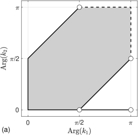
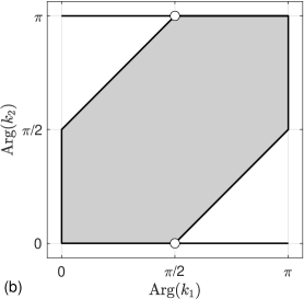
Figure 2: In each image, the gray region and the solid black lines constitute a set of points $({\rm{Arg}}(k_{1}),{\rm{Arg}}(k_{2}))$ for which, when $\kappa=k_{2}^{2}/k_{1}^{2}$, problem A has at most one solution and problem ${\sf A}_{0}$ only has the trivial solution. Dashed lines and circles are not included: (a) a set of points obtained using techniques from [16, 17]; (b) the set of points discussed in the second paragraph of Section 3.4.

3.4 Uniqueness and existence when $\kappa=k_{2}^{2}/k_{1}^{2}$

The parameter value $\kappa=k_{2}^{2}/k_{1}^{2}$ is relevant for the electromagnetic transmission problem. By using similar techniques as in [16, 17] one can show that when $\kappa=k_{2}^{2}/k_{1}^{2}$ and $({\rm{Arg}}(k_{1}),{\rm{Arg}}(k_{2}))$ is in the set of points of Figure 2(a), then problem A has at most one solution and problem ${\sf A}_{0}$ has only the trivial solution $U({\boldsymbol{r}})=0$.

We also mention that stronger results, including existence results, are available for problem A with (11) extended to $0\leq{\rm{Arg}}(k_{1}),{\rm{Arg}}(k_{2})\leq\pi$. Using methods from [1], developed for the more general Dirac equations, one can prove that problem A, with $\kappa=k_{2}^{2}/k_{1}^{2}$, has at most one solution in finite energy norm for $({\rm{Arg}}(k_{1}),{\rm{Arg}}(k_{2}))$ in the set of points of Figure 2(b). Furthermore, such a solution exists in Lipschitz domains given that $\kappa\notin[-c_{\Gamma},-1/c_{\Gamma}]$, where $c_{\Gamma}\geq 1$ is a geometry-dependent constant which assumes the value $c_{\Gamma}=1$ for smooth $\Gamma$ [13, Proposition 5.2].

4 Integral representations for problem A

We introduce two fields

$$U_{1}({\boldsymbol{r}}) =\frac{1}{2}K_{k_{1}}\mu({\boldsymbol{r}})-\frac{1}{2}S_{k_{1}}\varrho({\boldsymbol{r}})+U^{\rm in}({\boldsymbol{r}})\,,\quad{\boldsymbol{r}}\in\Omega_{1}\cup\Omega_{2}\,,$$ (26)

$$U_{2}({\boldsymbol{r}}) =-\frac{1}{2}K_{k_{2}}\mu({\boldsymbol{r}})+\frac{\kappa}{2}S_{k_{2}}\varrho({\boldsymbol{r}})\,,\quad{\boldsymbol{r}}\in\Omega_{1}\cup\Omega_{2}\,,$$ (27)

where $\mu$ and $\varrho$ are unknown surface densities. The relations in Section 2.2 give limits of $U_{1}({\boldsymbol{r}})$ and $U_{2}({\boldsymbol{r}})$ at ${\boldsymbol{r}}\in\Gamma$

$$U_{1}^{\pm}({\boldsymbol{r}}) =\pm\frac{1}{2}\mu({\boldsymbol{r}})+\frac{1}{2}K_{k_{1}}\mu({\boldsymbol{r}})-\frac{1}{2}S_{k_{1}}\varrho({\boldsymbol{r}})+U^{\rm in}({\boldsymbol{r}})\,,$$ (28)

$$U_{2}^{\pm}({\boldsymbol{r}}) =\mp\frac{1}{2}\mu({\boldsymbol{r}})-\frac{1}{2}K_{k_{2}}\mu({\boldsymbol{r}})+\frac{\kappa}{2}S_{k_{2}}\varrho({\boldsymbol{r}})\,.$$ (29)

Limits for the normal derivatives of $U_{1}({\boldsymbol{r}})$ and $U_{2}({\boldsymbol{r}})$ at ${\boldsymbol{r}}\in\Gamma$ are

$${\boldsymbol{\nu}}\cdot[\nabla U_{1}]^{\pm}({\boldsymbol{r}}) =\pm\frac{1}{2}\varrho({\boldsymbol{r}})+\frac{1}{2}T_{k_{1}}\mu({\boldsymbol{r}})-\frac{1}{2}K_{k_{1}}^{\rm A}\varrho({\boldsymbol{r}})+{\boldsymbol{\nu}}\cdot\nabla U^{\rm in}({\boldsymbol{r}})\,,$$ (30)

$${\boldsymbol{\nu}}\cdot[\nabla U_{2}]^{\pm}({\boldsymbol{r}}) =\mp\frac{\kappa}{2}\varrho({\boldsymbol{r}})-\frac{1}{2}T_{k_{2}}\mu({\boldsymbol{r}})+\frac{\kappa}{2}K_{k_{2}}^{\rm A}\varrho({\boldsymbol{r}})\,.$$ (31)

We now construct the ansatz

$$U({\boldsymbol{r}})=\left\{\begin{array}[]{ll}U_{1}({\boldsymbol{r}})\,,&{\boldsymbol{r}}\in\Omega_{1}\,,\\ U_{2}({\boldsymbol{r}})\,,&{\boldsymbol{r}}\in\Omega_{2}\,,\end{array}\right.$$ (32)

for the solution to problem A. The fundamental solution (3) makes $U$ of (32) automatically satisfy the PDEs of (12) and the radiation condition (15). It remains to determine $\mu$ and $\varrho$ to ensure that the boundary conditions (13) and (14) are satisfied.

5 Integral equations for problem A

We propose the system of second-kind integral equations on $\Gamma$

$$\begin{bmatrix}I-\beta_{1}(K_{k_{1}}-c_{1}K_{k_{2}})&\beta_{1}(S_{k_{1}}-c_{1}\kappa S_{k_{2}})\\ -\beta_{2}(T_{k_{1}}-c_{2}\kappa^{-1}T_{k_{2}})&I+\beta_{2}(K_{k_{1}}^{\rm A}-c_{2}K_{k_{2}}^{\rm A})\end{bmatrix}\begin{bmatrix}\mu\\ \varrho\end{bmatrix}=2\begin{bmatrix}\beta_{1}U^{\rm in}\\ \beta_{2}\partial_{\nu}U^{\rm in}\end{bmatrix}$$ (33)

for the determination of $\mu$ and $\varrho$. Here $I$ is the identity and

$$\beta_{i}=(1+c_{i})^{-1},\quad i=1,2\,,$$ (34)

where $c_{1}$ and $c_{2}$ are two free parameters such that

$$c_{i}\neq-1,0\,,\quad i=1,2\,.$$ (35)

We now prove that a solution $\{\mu,\varrho\}$ to (33), under certain conditions and via $U$ of (32), represents a solution to problem A. Since $U$ of (32) satisfies (12) and (15) for any $\{\mu,\varrho\}$, it remains to show that $\{\mu,\varrho\}$ from (33) makes $U$ satisfy (13) and (14). For this we need to show that, under certain conditions, $U_{1}$ of (26) is zero in $\Omega_{2}$ and $U_{2}$ of (27) is zero in $\Omega_{1}$. We introduce the auxiliary field

$$W({\boldsymbol{r}})=\left\{\begin{array}[]{ll}U_{2}({\boldsymbol{r}})\,,&{\boldsymbol{r}}\in\Omega_{1}\,,\\ -c_{1}^{-1}U_{1}({\boldsymbol{r}})\,,&{\boldsymbol{r}}\in\Omega_{2}\,.\end{array}\right.$$ (36)

The field $W$ of (36), with $\{\mu,\varrho\}$ from (33) and $U_{1}$ and $U_{2}$ from (26) and (27), is the unique solution to problem ${\sf B}_{0}$ with $\alpha=c_{2}/(c_{1}\kappa)$ provided that the conditions of Proposition 3.3 hold. This is so since $W$, by construction, satisfies (18) and (21). Furthermore, the boundary conditions (19) and (20) are satisfied. This can be checked by substituting $U_{1}^{-}$ of (28) and $U_{2}^{+}$ of (29) into (19), and ${\boldsymbol{\nu}}\cdot[\nabla U_{1}]^{-}$ of (30) and ${\boldsymbol{\nu}}\cdot[\nabla U_{2}]^{+}$ of (31) into (20), and using (33). As a consequence, according to Proposition 3.3, we have

$$W({\boldsymbol{r}})=0\,,\quad{\boldsymbol{r}}\in\Omega_{1}\cup\Omega_{2}\,.$$ (37)

Several useful results for ${\boldsymbol{r}}\in\Gamma$ follow from (36) and (37)

$$U_{1}^{-}({\boldsymbol{r}}) =0\,,$$ (38)

$$U_{2}^{+}({\boldsymbol{r}}) =0\,,$$ (39)

$${\boldsymbol{\nu}}\cdot[\nabla U_{1}]^{-}({\boldsymbol{r}}) =0\,,$$ (40)

$${\boldsymbol{\nu}}\cdot[\nabla U_{2}]^{+}({\boldsymbol{r}}) =0\,.$$ (41)

Now, from (28) and (38), and from (29) and (39)

$$U_{1}^{+}({\boldsymbol{r}}) =\mu({\boldsymbol{r}})\,,\quad{\boldsymbol{r}}\in\Gamma\,,$$ (42)

$$U_{2}^{-}({\boldsymbol{r}}) =\mu({\boldsymbol{r}})\,,\quad{\boldsymbol{r}}\in\Gamma\,.$$ (43)

Similarly, from (30) and (40), and from (31) and (41)

$${\boldsymbol{\nu}}\cdot[\nabla U_{1}]^{+}({\boldsymbol{r}}) =\varrho({\boldsymbol{r}})\,,\quad{\boldsymbol{r}}\in\Gamma\,,$$ (44)

$$\kappa^{-1}{\boldsymbol{\nu}}\cdot[\nabla U_{2}]^{-}({\boldsymbol{r}}) =\varrho({\boldsymbol{r}})\,,\quad{\boldsymbol{r}}\in\Gamma\,.$$ (45)

It is now easy to see that (13) and (14) are satisfied and we conclude:

Theorem 5.1.

Assume that $\{k_{1},k_{2},\alpha=c_{2}/(c_{1}\kappa)\}$ is such that the conditions of Proposition 3.3 hold. Then a solution $\{\mu,\varrho\}$ to (33) represents, via (32), a solution also to problem A. Furthermore, (32) and (33) correspond to a direct integral equation formulation of problem A with $\mu$ and $\varrho$ linked to limits of $U$ and $\nabla U$ via (42)–(45).

6 Unique solution to problem A from (33)

We use the Fredholm alternative to prove that, under certain conditions, the system (33) has a unique solution $\{\mu,\varrho\}$ and that this solution represents, via (32), the unique solution to problem A. Three conditions are referred to with roman numerals

• $c_{2}=\kappa$ and (35) holds.

• $k_{1}$, $k_{2}$, and $\kappa$ make the conditions of Proposition 3.1 or 3.2 hold or, if $\kappa=k_{2}^{2}/k_{1}^{2}$, $({\rm{Arg}}(k_{1}),{\rm{Arg}}(k_{2}))$ is in the set of points of Figure 2(a).

• $\{k_{1},k_{2},\alpha=c_{2}/(c_{1}\kappa)\}$ makes the conditions of Proposition 3.3 hold.

We start with the observation that (33) is a Fredholm second-kind integral equation with compact (differences of) operators when condition (i) holds and $\Gamma$ is smooth. Then the Fredholm alternative can be applied to (33). Let $\mu_{0}$ and $\varrho_{0}$ be solutions to the homogeneous version of (33). Let $U_{10}$, $U_{0}$, and $W_{0}$ be the fields (26), (32), and (36) with $\mu=\mu_{0}$ and $\varrho=\varrho_{0}$. From Section 5 we know that $W_{0}=0$ if (iii) holds. We shall now prove that also $U_{0}=0$ and, from that, $\mu_{0}=0$ and $\varrho_{0}=0$.

It follows from Theorem 5.1, which requires (iii), that $\{\mu_{0},\varrho_{0}\}$ represents a solution to problem ${\sf A}_{0}$. If (ii) holds, then $U_{0}=0$ according to Corollary 3.1. It then follows that $U_{10}=0$ in $\Omega_{1}$ so that $U_{10}^{+}=0$ and $[\nabla U_{10}]^{+}=0$. Then $\mu_{0}=0$ and $\varrho_{0}=0$ from (42) and (44). Now, from the Fredholm alternative, the system (33) has a unique solution $\{\mu,\varrho\}$. By Theorem 5.1 this solution represents a solution to problem A. If problem A has at most one solution, which requires (ii), this solution to problem A is unique and we conclude:

Theorem 6.1.

Assume that conditions (i), (ii), (iii) hold. Then the system (33) has a unique solution $\{\mu,\varrho\}$ which represents the unique solution to problem A.

Note that, when (i) holds, $\alpha=1/c_{1}$ in (iii) and it is always possible to find a constant $c_{1}$ so that (25) holds under the assumption (11). In this respect, condition (iii) in Theorem 6.1 does not introduce any additional constraint to problem A. A simple rule that satisfies condition (iii) is

$$c_{1}=\left\{\begin{array}[]{lll}e^{{\rm i}{\rm{Arg}}(k_{2})}&\mbox{if}&\Re{\rm e}\{k_{1}\}\geq 0\,,\\ e^{{\rm i}({\rm{Arg}}(k_{2})-\pi)}&\mbox{if}&\Re{\rm e}\{k_{1}\}<0\,.\end{array}\right.$$ (46)

This rule gives $c_{1}={\rm i}$ when $({\rm{Arg}}(k_{1}),{\rm{Arg}}(k_{2}))=(0,\pi/2)$. It is also possible to choose $c_{1}=-{\rm i}$ when $({\rm{Arg}}(k_{1}),{\rm{Arg}}(k_{2}))=(0,\pi/2)$.

Our results, so far, extend those of [16, Section 4.1], where a direct formulation of problem A is presented in [16, Eq. (4.10)]. To see this, note that [16, Eq. (4.10)] corresponds to (33) with $c_{2}=\kappa$ and $c_{1}=1/\kappa$. Now (33) with $c_{2}=\kappa$ and $c_{1}$ in agreement with (25) provides unique solutions over a broader range of $k_{1}$, $k_{2}$, and $\kappa$ than does [16, Eq. (4.10)]. For example, if $({\rm{Arg}}(k_{1}),{\rm{Arg}}(k_{2}))=(0,\pi/2)$ and ${\rm{Arg}}(\kappa)=\pi$, then (33) with $c_{2}=\kappa$ and $c_{1}=\pm{\rm i}$ is guaranteed to have a unique solution while [16, Eq. (4.10)] is not.

7 A weakly singular representation of $U$

Once the solution $\{\mu,\varrho\}$ has been obtained from (33), the field $U({\boldsymbol{r}})$ can be evaluated via (32). When ${\boldsymbol{r}}$ is close to $\Gamma$, this could be problematic due to the rapid variation with ${\boldsymbol{r}}^{\prime}$ in the Cauchy-type singular kernels of $K_{k_{1}}$ and $K_{k_{2}}$ in (26) and (27). To alleviate this problem we introduce

$$V({\boldsymbol{r}})=\left\{\begin{array}[]{ll}U_{2}({\boldsymbol{r}})\,,&{\boldsymbol{r}}\in\Omega_{1}\,,\\ U_{1}({\boldsymbol{r}})\,,&{\boldsymbol{r}}\in\Omega_{2}\,.\end{array}\right.$$ (47)

From (36) and (37) it follows that $V$ is a null-field such that $V=0$ in $\Omega_{1}\cup\Omega_{2}$, and hence $U=U+V$. The Cauchy-type kernel singularities in the representation of $U+V$ cancel out and we are left with better-behaved weakly singular kernels. In the numerical examples in Section 14 we exploit $U=U+V$ for near-field evaluation.

8 Electromagnetic transmission problems

We present three electromagnetic transmission problems called problem C, problem ${\sf C}_{0}$, and problem ${\sf D}_{0}$. The main problem is C, whereas problems ${\sf C}_{0}$ and ${\sf D}_{0}$ are needed in proofs.

The prerequisites in Section 2 hold, with regions $\Omega_{1}$ and $\Omega_{2}$ that are dielectric and non-magnetic. The electric field is denoted ${\boldsymbol{E}}$ and the magnetic field ${\boldsymbol{H}}$. The electric field is scaled such that ${\boldsymbol{E}}=\eta_{1}^{-1}{\boldsymbol{E}}_{\rm unscaled}$, where $\eta_{1}=\sqrt{\mu_{0}/\varepsilon_{1}}$ is the wave impedance of $\Omega_{1}$ and $\varepsilon_{1}$ is the permittivity of $\Omega_{1}$. Furthermore, problems C, ${\sf C}_{0}$, and ${\sf D}_{0}$ contain a complex parameter $\kappa$ which plays a somewhat similar role as the parameter $\kappa$ of Section 3.1 played in problem A and ${\sf A}_{0}$. This new $\kappa$ has the value $\kappa=\varepsilon_{2}/\varepsilon_{1}$, where $\varepsilon_{2}$ is the permittivity of $\Omega_{2}$. For non-magnetic materials, this is equivalent to

$$\kappa=k_{2}^{2}/k_{1}^{2}.$$ (48)

8.1 Problems C and ${\sf C}_{0}$

The transmission problem C reads: Given an incident field ${\boldsymbol{H}}^{\rm in}$, generated in $\Omega_{1}$, find ${\boldsymbol{E}}({\boldsymbol{r}}),\,{\boldsymbol{H}}({\boldsymbol{r}})$, ${\boldsymbol{r}}\in\Omega_{1}\cup\Omega_{2}$, which, for wavenumbers $k_{1}$ and $k_{2}$ and with $\kappa$ from (48) such that

$$0\leq{\rm{Arg}}(k_{1}),{\rm{Arg}}(k_{2})<\pi\quad\mbox{and}\quad\kappa\neq-1\,,$$ (49)

solve Maxwell’s equations

$$\begin{split}\nabla\times{\boldsymbol{E}}({\boldsymbol{r}})&={\rm i}k_{1}{\boldsymbol{H}}({\boldsymbol{r}})\,,\quad{\boldsymbol{r}}\in\Omega_{1}\cup\Omega_{2}\,,\\ \nabla\times{\boldsymbol{H}}({\boldsymbol{r}})&=-{\rm i}k_{1}{\boldsymbol{E}}({\boldsymbol{r}})\,,\quad{\boldsymbol{r}}\in\Omega_{1}\,,\\ \nabla\times{\boldsymbol{H}}({\boldsymbol{r}})&=-{\rm i}k_{1}\kappa{\boldsymbol{E}}({\boldsymbol{r}})\,,\quad{\boldsymbol{r}}\in\Omega_{2}\,,\end{split}$$ (50)

except possibly at an isolated point in $\Omega_{1}$ where the source of ${\boldsymbol{H}}^{\rm in}$ is located, subject to the boundary conditions

$${\boldsymbol{\nu}}\times{\boldsymbol{E}}^{+}({\boldsymbol{r}}) ={\boldsymbol{\nu}}\times{\boldsymbol{E}}^{-}({\boldsymbol{r}})\,,\quad{\boldsymbol{r}}\in\Gamma\,,$$ (51)

$${\boldsymbol{\nu}}\times{\boldsymbol{H}}^{+}({\boldsymbol{r}}) ={\boldsymbol{\nu}}\times{\boldsymbol{H}}^{-}({\boldsymbol{r}})\,,\quad{\boldsymbol{r}}\in\Gamma\,,$$ (52)

$$\left(\partial_{\hat{{\boldsymbol{r}}}}-{\rm i}k_{1}\right){\boldsymbol{H}}^{\rm sc}({\boldsymbol{r}}) =o\left(|{\boldsymbol{r}}|^{-1}\right),\quad\lvert{\boldsymbol{r}}\rvert\rightarrow\infty\,.$$ (53)

The scattered field ${\boldsymbol{H}}^{\rm sc}$ is source free in $\Omega_{1}$ and defined by

$${\boldsymbol{H}}({\boldsymbol{r}})={\boldsymbol{H}}^{\rm in}({\boldsymbol{r}})+{\boldsymbol{H}}^{\rm sc}({\boldsymbol{r}})\,,\quad{\boldsymbol{r}}\in\Omega_{1}\,.$$ (54)

The condition (53) and decomposition (54) also hold for ${\boldsymbol{E}}$. The incident field satisfies

$$\begin{split}\nabla\times{\boldsymbol{E}}^{\rm in}({\boldsymbol{r}})&={\rm i}k_{1}{\boldsymbol{H}}^{\rm in}({\boldsymbol{r}})\,,\quad{\boldsymbol{r}}\in\mathbb{R}^{3}\,,\\ \nabla\times{\boldsymbol{H}}^{\rm in}({\boldsymbol{r}})&=-{\rm i}k_{1}{\boldsymbol{E}}^{\rm in}({\boldsymbol{r}})\,,\quad{\boldsymbol{r}}\in\mathbb{R}^{3}\,,\end{split}$$ (55)

except at the possible isolated source point in $\Omega_{1}$.

The homogeneous problem ${\sf C}_{0}$ is problem C with ${\boldsymbol{E}}^{\rm in}={\boldsymbol{H}}^{\rm in}={\boldsymbol{0}}$.

8.2 Problem ${\sf D}_{0}$

The transmission problem ${\sf D}_{0}$ reads: find ${\boldsymbol{E}}_{W}({\boldsymbol{r}}),\,{\boldsymbol{H}}_{W}({\boldsymbol{r}})$, ${\boldsymbol{r}}\in\Omega_{1}\cup\Omega_{2}$, which, for a complex jump parameter $\lambda$ and for $k_{1}$, $k_{2}$, and $\kappa$ such that (49) holds, solve

$$\begin{split}\nabla\times{\boldsymbol{E}}_{W}({\boldsymbol{r}})&={\rm i}k_{1}{\boldsymbol{H}}_{W}({\boldsymbol{r}})\,,\quad{\boldsymbol{r}}\in\Omega_{1}\cup\Omega_{2}\,,\\ \nabla\times{\boldsymbol{H}}_{W}({\boldsymbol{r}})&=-{\rm i}k_{1}\kappa{\boldsymbol{E}}_{W}({\boldsymbol{r}})\,,\quad{\boldsymbol{r}}\in\Omega_{1}\,,\\ \nabla\times{\boldsymbol{H}}_{W}({\boldsymbol{r}})&=-{\rm i}k_{1}{\boldsymbol{E}}_{W}({\boldsymbol{r}})\,,\quad{\boldsymbol{r}}\in\Omega_{2}\,,\end{split}$$ (56)

subject to the boundary conditions

$$\lambda\kappa{\boldsymbol{\nu}}\times{\boldsymbol{E}}_{W}^{+}({\boldsymbol{r}}) ={\boldsymbol{\nu}}\times{\boldsymbol{E}}_{W}^{-}({\boldsymbol{r}})\,,\quad{\boldsymbol{r}}\in\Gamma\,,$$ (57)

$${\boldsymbol{\nu}}\times{\boldsymbol{H}}_{W}^{+}({\boldsymbol{r}}) ={\boldsymbol{\nu}}\times{\boldsymbol{H}}_{W}^{-}({\boldsymbol{r}})\,,\quad{\boldsymbol{r}}\in\Gamma\,,$$ (58)

$$\left(\partial_{\hat{{\boldsymbol{r}}}}-{\rm i}k_{2}\right){\boldsymbol{H}}_{W}({\boldsymbol{r}}) =o\left(|{\boldsymbol{r}}|^{-1}\right),\quad\lvert{\boldsymbol{r}}\rvert\rightarrow\infty\,.$$ (59)

The radiation condition (59) also holds for ${\boldsymbol{E}}_{W}$.

8.3 Uniqueness and existence of solutions to problem ${\sf C}$, ${\sf C}_{0}$, and ${\sf D}_{0}$

In Appendix D it is shown that when $({\rm{Arg}}(k_{1}),{\rm{Arg}}(k_{2}))$ is in the set of points of Figure 2(a), then problem C has at most one solution and problem ${\sf C}_{0}$ has only the trivial solution ${\boldsymbol{E}}={\boldsymbol{H}}={\boldsymbol{0}}$. It is also shown that when the conditions of Proposition 3.3 hold for $\{k_{1},k_{2},\alpha=\lambda\}$, then problem ${\sf D}_{0}$ has only the trivial solution ${\boldsymbol{E}}_{W}={\boldsymbol{H}}_{W}={\boldsymbol{0}}$.

The stronger results for problem A, discussed in Section 3.4, carry over to problem C. One can prove that there exists a unique solution in finite energy norm to problem C in Lipschitz domains when $({\rm{Arg}}(k_{1}),{\rm{Arg}}(k_{2}))$ is in the set of points of Figure 2(b) and $\kappa$ is outside a certain interval on the real axis [13, Proposition 7.4].

9 Integral representations for problem C

Let $\sigma_{\rm E}$, $\varrho_{\rm E}$, ${\boldsymbol{M}}_{\rm s}$, ${\boldsymbol{J}}_{\rm s}$, $\varrho_{\rm M}$, and $\sigma_{\rm M}$ be six unknown, scalar- and vector-valued, surface densities and define the four fields

$${\boldsymbol{E}}_{1}({\boldsymbol{r}}) =-\frac{1}{2}\boldsymbol{\cal N}_{k_{1}}\varrho_{\rm E}({\boldsymbol{r}})-\frac{1}{2}{\cal R}_{k_{1}}\left({\boldsymbol{\nu}}^{\prime}\sigma_{\rm M}+{\boldsymbol{M}}_{\rm s})({\boldsymbol{r}}\right)$$

$$\qquad+\frac{1}{2}\tilde{\cal S}_{k_{1}}({\boldsymbol{\nu}}^{\prime}\sigma_{\rm E}+{\boldsymbol{J}}_{\rm s})({\boldsymbol{r}})+{\boldsymbol{E}}^{\rm in}({\boldsymbol{r}})\,,\quad{\boldsymbol{r}}\in\Omega_{1}\cup\Omega_{2}\,,$$ (60)

$${\boldsymbol{E}}_{2}({\boldsymbol{r}}) =\frac{1}{2\kappa}\boldsymbol{\cal N}_{k_{2}}\varrho_{\rm E}({\boldsymbol{r}})+\frac{1}{2\kappa}{\cal R}_{k_{2}}\left({\boldsymbol{\nu}}^{\prime}\sigma_{\rm M}+\kappa{\boldsymbol{M}}_{\rm s})({\boldsymbol{r}}\right)$$

$$\qquad-\frac{1}{2}\tilde{\cal S}_{k_{2}}(\kappa^{-1}{\boldsymbol{\nu}}^{\prime}\sigma_{\rm E}+{\boldsymbol{J}}_{\rm s})({\boldsymbol{r}})\,,\quad{\boldsymbol{r}}\in\Omega_{1}\cup\Omega_{2}\,,$$ (61)

$${\boldsymbol{H}}_{1}({\boldsymbol{r}}) =\frac{1}{2}\tilde{\cal S}_{k_{1}}\left({\boldsymbol{\nu}}^{\prime}\sigma_{\rm M}+{\boldsymbol{M}}_{\rm s})({\boldsymbol{r}}\right)+\frac{1}{2}{\cal R}_{k_{1}}({\boldsymbol{\nu}}^{\prime}\sigma_{\rm E}+{\boldsymbol{J}}_{\rm s})({\boldsymbol{r}})$$

$$\qquad-\frac{1}{2}\boldsymbol{\cal N}_{k_{1}}\varrho_{\rm M}({\boldsymbol{r}})+{\boldsymbol{H}}^{\rm in}({\boldsymbol{r}})\,,\quad{\boldsymbol{r}}\in\Omega_{1}\cup\Omega_{2}\,,$$ (62)

$${\boldsymbol{H}}_{2}({\boldsymbol{r}}) =-\frac{1}{2}\tilde{\cal S}_{k_{2}}\left({\boldsymbol{\nu}}^{\prime}\sigma_{\rm M}+\kappa{\boldsymbol{M}}_{\rm s})({\boldsymbol{r}}\right)-\frac{1}{2}{\cal R}_{k_{2}}(\kappa^{-1}{\boldsymbol{\nu}}^{\prime}\sigma_{\rm E}+{\boldsymbol{J}}_{\rm s})({\boldsymbol{r}})$$

$$\qquad+\frac{1}{2}\boldsymbol{\cal N}_{k_{2}}\varrho_{\rm M}({\boldsymbol{r}})\,,\quad{\boldsymbol{r}}\in\Omega_{1}\cup\Omega_{2}\,.$$ (63)

The introduction of $\sigma_{\rm E}$ and $\sigma_{\rm M}$ is inspired by the integral representations for the generalized Helmholtz transmission problem in [26, 27].

The integral representations of the fields ${\boldsymbol{E}}$ and ${\boldsymbol{H}}$ for problem C are

$${\boldsymbol{E}}({\boldsymbol{r}})=\left\{\begin{array}[]{ll}{\boldsymbol{E}}_{1}({\boldsymbol{r}})\,,&{\boldsymbol{r}}\in\Omega_{1}\,,\\ {\boldsymbol{E}}_{2}({\boldsymbol{r}})\,,&{\boldsymbol{r}}\in\Omega_{2}\,,\end{array}\right.\quad{\boldsymbol{H}}({\boldsymbol{r}})=\left\{\begin{array}[]{ll}{\boldsymbol{H}}_{1}({\boldsymbol{r}})\,,&{\boldsymbol{r}}\in\Omega_{1}\,,\\ {\boldsymbol{H}}_{2}({\boldsymbol{r}})\,,&{\boldsymbol{r}}\in\Omega_{2}\,.\end{array}\right.$$ (64)

10 Integral equations for problem C

For the determination of $\{\sigma_{\rm E},\varrho_{\rm E},{\boldsymbol{M}}_{\rm s},{\boldsymbol{J}}_{\rm s},\varrho_{\rm M},\sigma_{\rm M}\}$ we propose the system of second-kind integral equations on $\Gamma$

$$\left(I+{\bf D}{\bf Q}\right){\boldsymbol{\mu}}=2{\bf D}{\boldsymbol{f}}\,.$$ (65)

Here ${\boldsymbol{\mu}}$ and ${\boldsymbol{f}}$ are column vectors with six entries each

$${\boldsymbol{\mu}} =\left[\sigma_{\rm E};\varrho_{\rm E};{\boldsymbol{M}}_{\rm s};{\boldsymbol{J}}_{\rm s};\varrho_{\rm M};\sigma_{\rm M}\right],$$

$${\boldsymbol{f}} =\left[0;{\boldsymbol{\nu}}\cdot{\boldsymbol{E}}^{\rm in};-{\boldsymbol{\nu}}\times{\boldsymbol{E}}^{\rm in};{\boldsymbol{\nu}}\times{\boldsymbol{H}}^{\rm in};{\boldsymbol{\nu}}\cdot{\boldsymbol{H}}^{\rm in};0\right],$$

${\bf Q}$ is a $6\times 6$ matrix whose non-zero operator entries $Q_{ij}$ map scalar- or vector-valued densities to scalar or vector-valued functions

$$Q_{11} =-K_{k_{1}}+c_{3}K_{k_{2}}\,,\quad Q_{12}=-\tilde{S}_{k_{1}}+c_{3}\kappa\tilde{S}_{k_{2}}\,,\quad Q_{14}=\nabla\cdot({\cal S}_{k_{1}}-c_{3}\kappa{\cal S}_{k_{2}})\,,$$

$$Q_{21} =-{\boldsymbol{\nu}}\cdot(\tilde{\cal S}_{k_{1}}-c_{4}\tilde{\cal S}_{k_{2}}){\boldsymbol{\nu}}^{\prime}\,,\quad Q_{22}=K_{k_{1}}^{\rm A}-c_{4}K_{k_{2}}^{\rm A}\,,$$

$$Q_{23} ={\boldsymbol{\nu}}\cdot({\cal R}_{k_{1}}-c_{4}\kappa{\cal R}_{k_{2}})\,,\quad Q_{24}=-{\boldsymbol{\nu}}\cdot(\tilde{\cal S}_{k_{1}}-c_{4}\kappa\tilde{\cal S}_{k_{2}})\,,$$

$$Q_{26} ={\boldsymbol{\nu}}\cdot({\cal R}_{k_{1}}-c_{4}{\cal R}_{k_{2}}){\boldsymbol{\nu}}^{\prime}\,,\quad Q_{31}={\boldsymbol{\nu}}\times(\tilde{\cal S}_{k_{1}}-c_{5}\kappa^{-1}\tilde{\cal S}_{k_{2}}){\boldsymbol{\nu}}^{\prime}\,,$$

$$Q_{32} =-{\boldsymbol{\nu}}\times(\boldsymbol{\cal N}_{k_{1}}-c_{5}\kappa^{-1}\boldsymbol{\cal N}_{k_{2}})\,,\quad Q_{33}=-{\boldsymbol{\nu}}\times({\cal R}_{k_{1}}-c_{5}{\cal R}_{k_{2}})\,,$$

$$Q_{34} ={\boldsymbol{\nu}}\times(\tilde{\cal S}_{k_{1}}-c_{5}\tilde{\cal S}_{k_{2}})\,,\quad Q_{36}=-{\boldsymbol{\nu}}\times({\cal R}_{k_{1}}-c_{5}\kappa^{-1}{\cal R}_{k_{2}}){\boldsymbol{\nu}}^{\prime}\,,$$

$$Q_{41} =-{\boldsymbol{\nu}}\times({\cal R}_{k_{1}}-c_{6}\kappa^{-1}{\cal R}_{k_{2}}){\boldsymbol{\nu}}^{\prime}\,,\quad Q_{43}=-{\boldsymbol{\nu}}\times(\tilde{\cal S}_{k_{1}}-c_{6}\kappa\tilde{\cal S}_{k_{2}})\,,$$

$$Q_{44} =-{\boldsymbol{\nu}}\times({\cal R}_{k_{1}}-c_{6}{\cal R}_{k_{2}})\,,\quad Q_{45}={\boldsymbol{\nu}}\times(\boldsymbol{\cal N}_{k_{1}}-c_{6}\boldsymbol{\cal N}_{k_{2}})\,,$$

$$Q_{46} =-{\boldsymbol{\nu}}\times(\tilde{\cal S}_{k_{1}}-c_{6}\tilde{\cal S}_{k_{2}}){\boldsymbol{\nu}}^{\prime}\,,\quad Q_{51}=-{\boldsymbol{\nu}}\cdot({\cal R}_{k_{1}}-c_{7}\kappa^{-1}{\cal R}_{k_{2}}){\boldsymbol{\nu}}^{\prime}\,,$$

$$Q_{53} =-{\boldsymbol{\nu}}\cdot(\tilde{\cal S}_{k_{1}}-c_{7}\kappa\tilde{\cal S}_{k_{2}})\,,\quad Q_{54}=-{\boldsymbol{\nu}}\cdot({\cal R}_{k_{1}}-c_{7}{\cal R}_{k_{2}})\,,$$

$$Q_{55} =K_{k_{1}}^{\rm A}-c_{7}K_{k_{2}}^{\rm A}\,,\quad Q_{56}=-{\boldsymbol{\nu}}\cdot(\tilde{\cal S}_{k_{1}}-c_{7}\tilde{\cal S}_{k_{2}}){\boldsymbol{\nu}}^{\prime}\,,$$

$$Q_{63} =\nabla\cdot({\cal S}_{k_{1}}-c_{8}\kappa{\cal S}_{k_{2}})\,,\quad Q_{65}=-\tilde{S}_{k_{1}}+c_{8}\kappa\tilde{S}_{k_{2}}\,,\quad Q_{66}=-K_{k_{1}}+c_{8}K_{k_{2}}\,,$$

${\bf D}$ is a diagonal $6\times 6$ matrix of scalars with non-zero entries

$$\begin{split}&D_{ii}=(1+c_{i+2})^{-1}\,,\quad i=1,\ldots,6\,,\\ c_{3}=&\gamma_{\rm E}c\,,\quad c_{4}=c_{6}=c\,,\quad c_{5}=c_{7}=\lambda\kappa c\,,\quad c_{8}=\gamma_{\rm M}c\,,\end{split}$$ (66)

and $c$, $\lambda$, $\gamma_{\rm E}$, and $\gamma_{\rm M}$ are free parameters such that

$$c_{i}\neq-1,0,\quad i=3,\ldots,8\,.$$ (67)

10.1 Criteria for (64) to represent a solution to problem C

We now prove that a solution ${\boldsymbol{\mu}}$ to (65), under certain conditions and via (64), represents a solution to problem C.

The fundamental solution (3) makes ${\boldsymbol{E}}$ and ${\boldsymbol{H}}$ of (64) satisfy the radiation condition (53). It remains to prove that ${\boldsymbol{E}}$ and ${\boldsymbol{H}}$ satisfy Maxwell’s equations (50) and the boundary conditions (51) and (52). For this we first need to show that, under certain conditions, ${\boldsymbol{E}}_{1}$ and ${\boldsymbol{H}}_{1}$ of (60) and (62) are zero in $\Omega_{2}$ and ${\boldsymbol{E}}_{2}$ and ${\boldsymbol{H}}_{2}$ of (61) and (63) are zero in $\Omega_{1}$. We introduce the auxiliary fields

$${\boldsymbol{E}}_{W}({\boldsymbol{r}})=\left\{\begin{array}[]{ll}{\boldsymbol{E}}_{2}({\boldsymbol{r}})\,,&{\boldsymbol{r}}\in\Omega_{1}\,,\\ -c^{-1}{\boldsymbol{E}}_{1}({\boldsymbol{r}})\,,&{\boldsymbol{r}}\in\Omega_{2}\,,\end{array}\right.\quad{\boldsymbol{H}}_{W}({\boldsymbol{r}})=\left\{\begin{array}[]{ll}{\boldsymbol{H}}_{2}({\boldsymbol{r}})\,,&{\boldsymbol{r}}\in\Omega_{1}\,,\\ -c^{-1}{\boldsymbol{H}}_{1}({\boldsymbol{r}})\,,&{\boldsymbol{r}}\in\Omega_{2}\,.\end{array}\right.$$ (68)

The fields ${\boldsymbol{E}}_{W}$ and ${\boldsymbol{H}}_{W}$, with ${\boldsymbol{\mu}}$ from (65), is the unique trivial solution to problem ${\sf D}_{0}$ provided the sets $\{k_{1},k_{2},\alpha=\lambda\bar{\gamma}_{\rm M}\}$, $\{k_{1},k_{2},\alpha=\bar{\gamma}_{\rm E}\bar{\kappa}\}$, and $\{k_{1},k_{2},\alpha=\lambda\}$ are such that the conditions of Proposition 3.3 hold. This statement is now shown in several steps. The fundamental solution (3) makes ${\boldsymbol{E}}_{W}$ and ${\boldsymbol{H}}_{W}$ satisfy (59). Using Appendix A in combination with (65) one can show that (57) and (58) are satisfied. Appendix B shows that if ${\boldsymbol{\mu}}$ is a solution to (65) and if the conditions of Proposition 3.3 hold for $\{k_{1},k_{2},\alpha=\lambda\bar{\gamma}_{\rm M}\}$ and $\{k_{1},k_{2},\alpha=\bar{\gamma}_{\rm E}\bar{\kappa}\}$, then

$$\nabla\cdot{\boldsymbol{E}}_{W}({\boldsymbol{r}}) =0\,,\quad{\boldsymbol{r}}\in\Omega_{1}\cup\Omega_{2}\,,$$ (69)

$$\nabla\cdot{\boldsymbol{H}}_{W}({\boldsymbol{r}}) =0\,,\quad{\boldsymbol{r}}\in\Omega_{1}\cup\Omega_{2}\,.$$ (70)

Appendix C shows that if (69) and (70) hold, then ${\boldsymbol{E}}_{W}$ and ${\boldsymbol{H}}_{W}$ satisfy (56). If the conditions of Proposition 3.3 also hold for $\{k_{1},k_{2},\alpha=\lambda\}$, then ${\sf D}_{0}$ only has the trivial solution ${\boldsymbol{E}}_{W}={\boldsymbol{H}}_{W}={\boldsymbol{0}}$, that is,

$$\begin{split}{\boldsymbol{E}}_{2}({\boldsymbol{r}})&={\boldsymbol{H}}_{2}({\boldsymbol{r}})={\boldsymbol{0}}\,,\quad{\boldsymbol{r}}\in\Omega_{1}\,,\\ {\boldsymbol{E}}_{1}({\boldsymbol{r}})&={\boldsymbol{H}}_{1}({\boldsymbol{r}})={\boldsymbol{0}}\,,\quad{\boldsymbol{r}}\in\Omega_{2}\,.\end{split}$$ (71)

By that the statement is proven.

From (71) and Appendix A we obtain the surface densities as boundary values of the full 3D electromagnetic fields

$$[\nabla\cdot{\boldsymbol{E}}_{1}]^{+}({\boldsymbol{r}}) =\kappa[\nabla\cdot{\boldsymbol{E}}_{2}]^{-}({\boldsymbol{r}})=-{\rm i}k_{1}\sigma_{\rm E}({\boldsymbol{r}})\,,$$ (72)

$${\boldsymbol{\nu}}\cdot{\boldsymbol{E}}_{1}^{+}({\boldsymbol{r}}) =\kappa{\boldsymbol{\nu}}\cdot{\boldsymbol{E}}_{2}^{-}({\boldsymbol{r}})=\varrho_{\rm E}({\boldsymbol{r}})\,,$$ (73)

$${\boldsymbol{\nu}}\times{\boldsymbol{E}}_{1}^{+}({\boldsymbol{r}}) ={\boldsymbol{\nu}}\times{\boldsymbol{E}}_{2}^{-}({\boldsymbol{r}})=-{\boldsymbol{M}}_{\rm s}({\boldsymbol{r}})\,,$$ (74)

$${\boldsymbol{\nu}}\times{\boldsymbol{H}}_{1}^{+}({\boldsymbol{r}}) ={\boldsymbol{\nu}}\times{\boldsymbol{H}}_{2}^{-}({\boldsymbol{r}})={\boldsymbol{J}}_{\rm s}({\boldsymbol{r}})\,,$$ (75)

$${\boldsymbol{\nu}}\cdot{\boldsymbol{H}}_{1}^{+}({\boldsymbol{r}}) ={\boldsymbol{\nu}}\cdot{\boldsymbol{H}}_{2}^{-}({\boldsymbol{r}})=\varrho_{\rm M}({\boldsymbol{r}})\,,$$ (76)

$$[\nabla\cdot{\boldsymbol{H}}_{1}]^{+}({\boldsymbol{r}}) =[\nabla\cdot{\boldsymbol{H}}_{2}]^{-}({\boldsymbol{r}})=-{\rm i}k_{1}\sigma_{\rm M}({\boldsymbol{r}})\,.$$ (77)

Due to (74) and (75), ${\boldsymbol{E}}$ and ${\boldsymbol{H}}$ of (64) satisfy (51) and (52). Appendix B shows that (72)–(77) imply

$$\nabla\cdot{\boldsymbol{E}}({\boldsymbol{r}})=\nabla\cdot{\boldsymbol{H}}({\boldsymbol{r}})=0\,,\quad{\boldsymbol{r}}\in\Omega_{1}\cup\Omega_{2}\,,$$ (78)

when $({\rm{Arg}}(k_{1}),{\rm{Arg}}(k_{2}))$ is in the set of points of Figure 2(a). Finally, from the representations (60)–(63) and the divergence condition (78), Appendix C shows that (50) is satisfied. We conclude:

Theorem 10.1.

Assume that $\{k_{1},k_{2},\alpha=\lambda\bar{\gamma}_{\rm M}\}$, $\{k_{1},k_{2},\alpha=\bar{\gamma}_{\rm E}\bar{\kappa}\}$, and $\{k_{1},k_{2},\alpha=\lambda\}$ are such that the conditions of Proposition 3.3 hold. Then a solution ${\boldsymbol{\mu}}$ to (65) represents, via (64), a solution also to problem C. Furthermore, (64) and (65) correspond to a direct integral equation formulation of problem C with ${\boldsymbol{\mu}}$ linked to limits of ${\boldsymbol{E}}$ and ${\boldsymbol{H}}$ via (72)–(77).

Remark 10.1.

The surface densities in (72)–(77) can be given the following physical interpretations: $-{\rm i}k_{1}\sigma_{\rm E}$ and $-{\rm i}k_{1}\sigma_{\rm M}$ are the electric and magnetic volume charge densities at $\Gamma^{+}$, $\varrho_{\rm E}$ and $\varrho_{\rm M}$ are the equivalent electric and magnetic surface charge densities on $\Gamma^{+}$, and ${\boldsymbol{M}}_{\rm s}$ and ${\boldsymbol{J}}_{\rm s}$ are the equivalent magnetic and electric surface current densities on $\Gamma^{+}$.

11 Unique solution to problem C from (65)

We now prove that if there exists a solution to problem C, then, under certain conditions, there exists a solution ${\boldsymbol{\mu}}$ to (65) and it represents the unique solution to problem C. Three conditions are referred to

• The conditions in (67) hold.

• $({\rm{Arg}}(k_{1}),{\rm{Arg}}(k_{2}))$ is in the set of points of Figure 2(a).

• $\{k_{1},k_{2},\alpha=\lambda\bar{\gamma}_{\rm M}\}$, $\{k_{1},k_{2},\alpha=\bar{\gamma}_{\rm E}\bar{\kappa}\}$, and $\{k_{1},k_{2},\alpha=\lambda\}$ are such that the conditions of Proposition 3.3 hold.

Let ${\boldsymbol{\mu}}_{0}$ be a solution to the homogeneous version of (65) and assume that (i), (ii), and (iii) hold. Since (iii) holds, ${\boldsymbol{\mu}}_{\rm 0}$ represents a solution to problem C₀, according to Theorem 10.1. Since (ii) holds, this solution is the trivial solution ${\boldsymbol{E}}={\boldsymbol{H}}={\boldsymbol{0}}$, according to Section 8.3. The limits of fields in (72)–(77) are then zero and hence ${\boldsymbol{\mu}}_{0}={\boldsymbol{0}}$. Then (65) has at most one solution ${\boldsymbol{\mu}}$. Since ${\boldsymbol{\mu}}$ is linked to limits of ${\boldsymbol{E}}$ and ${\boldsymbol{H}}$ via (72)–(77) it follows that if problem C has a solution, then via (72)–(77) this solution gives a ${\boldsymbol{\mu}}$ that solves (65). We conclude:

Theorem 11.1.

Assume that there exists a solution to problem C and that condition (ii) holds. Then this solution is unique. If conditions (i) and (iii) also hold, then there exists a unique solution ${\boldsymbol{\mu}}$ to (65) and this solution represents via (64) the unique solution to problem C.

Remark 11.1.

From (72), (77), and (78) it is seen that $\sigma_{\rm E}$ and $\sigma_{\rm M}$ are zero. Despite this, $\sigma_{\rm E}$ and $\sigma_{\rm M}$ are needed in (65) to guarantee uniqueness. Often, however, one can omit $\sigma_{\rm E}$ and $\sigma_{\rm M}$ from (65) and still get the correct unique solution.

11.1 Determination of uniqueness parameters

The system (65) contains the free parameters $\lambda$, $\gamma_{\rm E}$, $\gamma_{\rm M}$, and $c$. Unique solvability of (65) requires that the conditions of Proposition 3.3 hold for the sets $\{k_{1},k_{2},\alpha=\lambda\bar{\gamma}_{\rm M}\}$, $\{k_{1},k_{2},\alpha=\bar{\gamma}_{\rm E}\bar{\kappa}\}$, and $\{k_{1},k_{2},\alpha=\lambda\}$ while the choice of $c$ is restricted by (67). Because of their role in ensuring unique solvability of (65), we refer to $\{\lambda,\gamma_{\rm E},\gamma_{\rm M},c\}$ as uniqueness parameters.

Generally, there are many parameter choices for which the conditions of Proposition 3.3 and (67) hold for a given $\{k_{1},k_{2}\}$ satisfying (11). A valid choice, which also works well numerically, when ${\rm{Arg}}(k_{1})=0$ and $\pi/4\leq{\rm{Arg}}(k_{2})\leq\pi/2$ is

$$\lambda=e^{-{\rm i}{\rm{Arg}}(k_{2})},\quad\gamma_{\rm E}=\kappa^{-1}e^{{\rm i}({\rm{Arg}}(k_{2})-\pi)},\quad\gamma_{\rm M}=1\,,\quad c=\lambda^{-1},$$ (79)

and when ${\rm{Arg}}(k_{1})=0$ and $\pi/2\leq{\rm{Arg}}(k_{2})\leq 3\pi/4$

$$\lambda=e^{{\rm i}(\pi-{\rm{Arg}}(k_{2}))},\quad\gamma_{\rm E}=\kappa^{-1}e^{{\rm i}{\rm{Arg}}(k_{2})},\quad\gamma_{\rm M}=1\,,\quad c=\lambda^{-1}.$$ (80)

12 2D limits

As a first numerical test of our formulations we consider, in Section 14, the 2D transverse magnetic (TM) transmission problem where an incident TM wave is scattered from an infinite cylinder. This problem is independent of the $z$-coordinate and we introduce the vector $r=(x,y)$, the unit tangent vector $\tau=(\tau_{x},\tau_{y})$, and the unit normal vector $\nu=(\nu_{x},\nu_{y})$, where $(\tau_{x},\tau_{y},0)=\hat{{\boldsymbol{z}}}\times(\nu_{x},\nu_{y},0)$ and $\hat{{\boldsymbol{z}}}$ is the unit vector in the $z$-direction. The incident wave has polarization ${\boldsymbol{H}}^{\rm in}(r)=\hat{{\boldsymbol{z}}}H^{\rm in}(r)$, which implies ${\boldsymbol{M}}_{\rm s}=\hat{{\boldsymbol{z}}}M$, ${\boldsymbol{J}}_{\rm s}=\tau J$, $\varrho_{\rm M}=0$, and $\sigma_{\rm M}=0$.

The integral representations (26), (27), and (60)–(63), as well as the systems (33) and (65), are transferred to two dimensions by exchanging the fundamental solution (3) for the 2D fundamental solution

$$\Phi_{k}(r,r^{\prime})=\frac{\rm i}{4}H_{0}^{(1)}(k|r-r^{\prime}|)\,,\quad r,r^{\prime}\in\mathbb{R}^{2},$$ (81)

where $H_{0}^{(1)}$ is the zeroth order Hankel function of the first kind.

12.1 Integral representations in two dimensions

Since $\sigma_{\rm E}$ is zero, see Remark 11.1, the 2D representation of the field ${\boldsymbol{H}}$ in (64), to be used in evaluation of the magnetic field, is

$$H(r)=\left\{\begin{array}[]{ll}\dfrac{1}{2}\tilde{S}_{k_{1}}M(r)-\dfrac{1}{2}K_{k_{1}}J(r)+H^{\rm in}(r)\,,&r\in\Omega_{1}\,,\\ -\dfrac{\kappa}{2}\tilde{S}_{k_{2}}M(r)+\dfrac{1}{2}K_{k_{2}}J(r)\,,&r\in\Omega_{2}\,.\end{array}\right.$$ (82)

By letting $U=H$, $U^{\rm in}=H^{\rm in}$, $\mu=-J$, $\varrho=-{\rm i}k_{1}M$, and $\kappa=k_{2}^{2}/k_{1}^{2}$ in the scalar representation (32) it becomes identical to (82). According to Section 7 one may add null-fields to (82). That gives the representation

$$H(r)=\frac{1}{2}(\tilde{S}_{k_{1}}-\kappa\tilde{S}_{k_{2}})M(r)-\frac{1}{2}(K_{k_{1}}-K_{k_{2}})J(r)+H^{\rm in}(r)\,,\quad r\in\Omega_{1}\cup\Omega_{2},$$ (83)

which is to prefer for evaluations at points $r$ close to $\Gamma$.

12.2 Integral equations with four, three, and two densities

In the TM problem the system (65) becomes

$$\left(I+\tilde{\bf D}\tilde{\bf Q}\right)\tilde{{\boldsymbol{\mu}}}=2\tilde{\bf D}\tilde{{\boldsymbol{f}}}\,.$$ (84)

Here $\tilde{{\boldsymbol{\mu}}}$ and $\tilde{{\boldsymbol{f}}}$ are column vectors with four entries each

$$\tilde{{\boldsymbol{\mu}}} =\left[\sigma_{\rm E};\varrho_{\rm E};M;J\right],$$

$$\tilde{{\boldsymbol{f}}} =\left[0;{\rm i}k_{1}^{-1}\partial_{\tau}H^{\rm in};{\rm i}k_{1}^{-1}\partial_{\nu}H^{\rm in};-H^{\rm in}\right],$$

$\tilde{\bf Q}$ is a $4\times 4$ matrix with non-zero scalar operator entries

$$\tilde{Q}_{11} =-K_{k_{1}}+c_{3}K_{k_{2}}\,,\quad\tilde{Q}_{12}=-\tilde{S}_{k_{1}}+c_{3}\kappa\tilde{S}_{k_{2}}\,,\quad\tilde{Q}_{14}=-C_{k_{1}}+c_{3}\kappa C_{k_{2}}\,,$$

$$\tilde{Q}_{21} =-(\tilde{S}_{k_{1}}-c_{4}\tilde{S}_{k_{2}})\nu\cdot\nu^{\prime}\,,\quad\tilde{Q}_{22}=K_{k_{1}}^{\rm A}-c_{4}K_{k_{2}}^{\rm A}\,,$$

$$\tilde{Q}_{23} =C_{k_{1}}^{\rm A}-c_{4}\kappa C_{k_{2}}^{\rm A}\,,\quad\tilde{Q}_{24}=-(\tilde{S}_{k_{1}}-c_{4}\kappa\tilde{S}_{k_{2}})\nu\cdot\tau^{\prime}\,,$$

$$\tilde{Q}_{31} =(\tilde{S}_{k_{1}}-c_{5}\kappa^{-1}\tilde{S}_{k_{2}})\tau\cdot\nu^{\prime}\,,\quad\tilde{Q}_{32}=-C_{k_{1}}^{\rm A}+c_{5}\kappa^{-1}C_{k_{2}}^{\rm A}\,,$$

$$\tilde{Q}_{33} =K_{k_{1}}^{\rm A}-c_{5}K_{k_{2}}^{\rm A}\,,\quad\tilde{Q}_{34}=(\tilde{S}_{k_{1}}-c_{5}\tilde{S}_{k_{2}})\tau\cdot\tau^{\prime}\,,$$

$$\tilde{Q}_{41} =C_{k_{1}}-c_{6}\kappa^{-1}C_{k_{2}}\,,\quad\tilde{Q}_{43}=\tilde{S}_{k_{1}}-c_{6}\kappa\tilde{S}_{k_{2}}\,,\quad\tilde{Q}_{44}=-K_{k_{1}}+c_{6}K_{k_{2}}\,,$$

$\tilde{\bf D}$ is a diagonal $4\times 4$ matrix of scalars with non-zero entries

$$\tilde{D}_{ii}=(1+c_{i+2})^{-1}\,,\quad i=1,2,3,4\,,$$

and

$$\begin{split}C_{k}\sigma(r)&=2\int_{\Gamma}(\partial_{\tau^{\prime}}\Phi_{k})(r,r^{\prime})\sigma(r^{\prime})\,{\rm d}\Gamma^{\prime},\quad r\in\Gamma\,,\\ C_{k}^{\rm A}\sigma(r)&=2\int_{\Gamma}(\partial_{\tau}\Phi_{k})(r,r^{\prime})\sigma(r^{\prime})\,{\rm d}\Gamma^{\prime},\quad r\in\Gamma.\end{split}$$ (85)

If we omit $\sigma_{\rm E}$, see Remark 11.1, the system (84) reduces to

$$\left(I+\hat{\bf D}\hat{\bf Q}\right)\hat{{\boldsymbol{\mu}}}=2\hat{\bf D}\hat{{\boldsymbol{f}}}\,.$$ (86)

Here $\hat{\bf Q}$ and $\hat{\bf D}$ are $\tilde{\bf Q}$ and $\tilde{\bf D}$ with the first row and column deleted, $\hat{{\boldsymbol{f}}}$ is $\tilde{{\boldsymbol{f}}}$ with the first entry deleted, and $\hat{{\boldsymbol{\mu}}}$ contains the three densities $\{\varrho_{\rm E},M,J\}$.

A third alternative is to only use the densities $M$ and $J$. The integral representation (32) and system (33) are now suitable, where the change of variables in Section 12.1 makes (32) equal to (82) and (33) equal to

$$\begin{bmatrix}I+\beta_{2}(K_{k_{1}}^{\rm A}-c_{2}K_{k_{2}}^{\rm A})&\beta_{2}{\rm i}k_{1}^{-1}(T_{k_{1}}-c_{2}\kappa^{-1}T_{k_{2}})\\ \beta_{1}(\tilde{S}_{k_{1}}-c_{1}\kappa\tilde{S}_{k_{2}})&I-\beta_{1}(K_{k_{1}}-c_{1}K_{k_{2}})\end{bmatrix}\begin{bmatrix}M\\ J\end{bmatrix}=2\begin{bmatrix}\beta_{2}{\rm i}k_{1}^{-1}\partial_{\nu}H^{\rm in}\\ -\beta_{1}H^{\rm in}\end{bmatrix}.$$ (87)

If the conditions in Theorem 6.1 hold, then (87) has a unique solution $\{M,J\}$. Via (82) it represents the unique solution to the 2D TM problem.

13 Test domains and discretization

This section reviews domains and discretization schemes that are used for numerical tests in the next section.

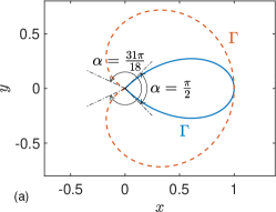
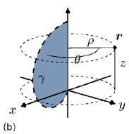
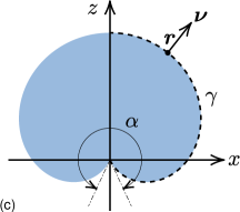
Figure 3: Non-smooth test domains: (a) boundaries $\Gamma$ of 2D domains with corner opening angles $\alpha=\pi/2$ (solid blue) and $\alpha=31\pi/18$ (dashed orange); (b) cylindrical coordinates $(\rho,\theta,z)$ of a point ${\boldsymbol{r}}$ on the surface of an axisymmetric object with generating curve $\gamma$; (c) cross section of the object generated by $\gamma$ with conical point opening angle $\alpha=31\pi/18$.

13.1 The 2D one-corner object and the 3D “tomato”

Numerical tests in two dimensions involve a one-corner object whose boundary $\Gamma$ is parameterized as

$$r(s)=\sin(\pi s)\left(\cos((s-0.5)\alpha),\sin((s-0.5)\alpha)\right)\,,\quad s\in[0,1]\,,$$ (88)

and where $\alpha$ is a corner opening angle. See Figure 3(a) for illustrations.

Numerical tests in three dimensions involve an object whose surface $\Gamma$ is created by revolving the generating curve $\gamma$, parameterized as

$${\boldsymbol{r}}(s)=\sin(\pi s)\left(\sin((0.5-s)\alpha),0,\cos((0.5-s)\alpha)\right)\,,\quad s\in[0,0.5]\,,$$ (89)

around the $z$-axis. For $\alpha>\pi$ this object resembles a “tomato”. See Figure 1 and Figure 3(b,c) for illustrations with $\alpha=31\pi/18$.

The reason for testing integral equations in axisymmetric domains, rather than in general domains, is the availability of efficient high-order solvers. Use of axisymmetric domains and solvers as a robust test-bed for new integral equation reformulations of scattering problems is contemporary common practice [6, 18].

13.2 RCIP-accelerated Nyström discretization schemes

Nyström discretization, relying on composite Gauss–Legendre quadrature, is used for all our systems of integral equations. Large discretized linear systems are solved iteratively using GMRES. In the presence of singular boundary points which call for intense mesh refinement, the Nyström scheme is accelerated by recursively compressed inverse preconditioning (RCIP) [8]. The RCIP acts as a fully automated, geometry-independent, and fast direct local solver and boosts the performance of the original Nyström scheme to the point where problems on non-smooth $\Gamma$ are solved with the same ease as on smooth $\Gamma$. Accurate evaluations of layer potentials close to their sources on $\Gamma$ are accomplished using variants of the techniques first presented in [7].

The schemes used in the numerical examples are not entirely new. For 2D problems we use the scheme in [11, Section 11.3], relying on 16-point composite quadrature. For 3D problems we use a modified unification of the schemes in [9] and [12], relying on 32-point composite quadrature. A key feature in the scheme of [9] is an FFT-accelerated separation of variables, pioneered by [28] and used also in [6, 18].

An important technique in [9] is the split of the numerator in $\Phi_{k}({\boldsymbol{r}},{\boldsymbol{r}}^{\prime})$ of (3) into parts that are even and odd in $\lvert{\boldsymbol{r}}-{\boldsymbol{r}}^{\prime}\rvert$. Let $G(k,{{\boldsymbol{r}}},{{\boldsymbol{r}}}^{\prime})$ be one of the $2\pi$-periodic kernels of Section 2.1. Azimuthal Fourier coefficients

$$G_{n}=\frac{1}{\sqrt{2\pi}}\int_{-\pi}^{\pi}e^{-{\rm i}n(\theta-\theta^{\prime})}G(k,{{\boldsymbol{r}}},{{\boldsymbol{r}}}^{\prime})\,{\rm d}(\theta-\theta^{\prime})\,,\quad n=0,\pm 1,\pm 2,\ldots\,,$$ (90)

are, for ${\boldsymbol{r}}$ and ${\boldsymbol{r}}^{\prime}$ close to each other, computed in different ways depending on the parity of these parts. When $\Im{\rm m}\{k\}$ is small, the split

$$e^{{\rm i}k\lvert{\boldsymbol{r}}-{\boldsymbol{r}}^{\prime}\rvert}=\cos(k\lvert{\boldsymbol{r}}-{\boldsymbol{r}}^{\prime}\rvert)+{\rm i}\sin(k\lvert{\boldsymbol{r}}-{\boldsymbol{r}}^{\prime}\rvert)$$ (91)

is efficient for $\Phi_{k}({\boldsymbol{r}},{\boldsymbol{r}}^{\prime})$. When $\Im{\rm m}\{k\}$ is large, the terms on the right hand side of (91) can be much larger in modulus than the function on the left hand side. Then numerical cancellation takes place. To fix this problem for large $\Im{\rm m}\{k\}$, not encountered in [9], we introduce a bump-like function

$$\chi(k,\lvert{\boldsymbol{r}}-{\boldsymbol{r}}^{\prime}\rvert)=e^{-\left(\Im{\rm m}\{k\}{\lvert{\boldsymbol{r}}-{\boldsymbol{r}}^{\prime}\rvert/4.6}\right)^{8}}\,,$$ (92)

modify the split (91) to

$$e^{{\rm i}k\lvert{\boldsymbol{r}}-{\boldsymbol{r}}^{\prime}\rvert}=(1-\chi)e^{{\rm i}k\lvert{\boldsymbol{r}}-{\boldsymbol{r}}^{\prime}\rvert}+\chi\cos(k\lvert{\boldsymbol{r}}-{\boldsymbol{r}}^{\prime}\rvert)+{\rm i}\chi\sin(k\lvert{\boldsymbol{r}}-{\boldsymbol{r}}^{\prime}\rvert)\,,$$ (93)

and compute $G_{n}$ of (90) with techniques (direct transform or convolution) appropriate for parts of $G(k,{{\boldsymbol{r}}},{{\boldsymbol{r}}}^{\prime})$ associated with each of the terms on the right hand side of (93).

14 Numerical examples

The systems (65), (84), (86), and (87) and the representations (64), (82), and (83) are now put to the test. In all examples we take $k_{1}$ real and positive, $\varepsilon_{1}=1$, and $\varepsilon_{2}=-1.1838$. This parameter combination satisfies the plasmonic condition (1) and has been used in previous work on 2D surface plasmon waves [2, 10, 11]. In situations involving non-smooth surfaces, it may happen that solutions for $\varepsilon_{2}=-1.1838$ do not exist. We then compute limit solutions as $\varepsilon_{2}$ approaches $-1.1838$ from above in the complex plane. Such limit solutions, discussed in the context of Laplace transmission problems in [12, Section 2.2], have boundary traces that may best be characterized as lying in fractional-order Sobolev spaces [13] and are given a downarrow superscript. For example, the limit of the field ${\boldsymbol{H}}$ is denoted ${\boldsymbol{H}}^{\downarrow}$. The uniqueness parameters $\{\lambda,\gamma_{\rm E},\gamma_{\rm M},c\}$, needed in (65), (84), and (86), are chosen according to (80). The uniqueness parameters needed in (87) are chosen as $\{c_{1},c_{2}\}=\{-{\rm i},\kappa\}$.

Our codes are implemented in Matlab, release 2018b, and executed on a workstation equipped with an Intel Core i7-3930K CPU and 64 GB of RAM. When assessing the accuracy of computed field quantities we most often adopt a procedure where to each numerical solution we also compute an overresolved reference solution, using roughly 50% more points in the discretization of the system under study. The absolute difference between these two solutions is denoted the estimated absolute error. Throughout the examples, field quantities are computed at $10^{6}$ field points on a rectangular Cartesian grid in the computational domains shown in the figures.

14.1 Unique solvability on the unit circle

We compute condition numbers of the discretized system matrices in (84), (86), and (87). The boundary $\Gamma$ is the unit circle and $k_{1}$ is swept through the interval $[0,10]$. Recall that the systems (84) and (87) are guaranteed to be free from wavenumbers for which the solution is not unique (false eigenwavenumbers) while the system (86) is not.

Condition number analysis of 2D limits of 3D systems on the unit circle is a revealing test for detecting if a given system of integral equations has false eigenwavenumbers when the plasmonic condition holds. For example, in [11, Figure 9] it is shown that the original Müller system and the “${\boldsymbol{E}}$-system” of [27] exhibit several false eigenwavenumbers in such a test.

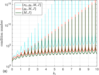
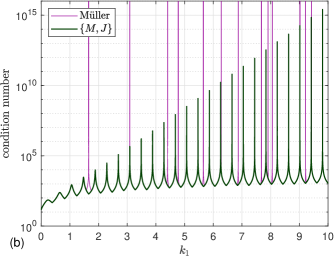
Figure 4: Condition numbers of system matrices on the unit circle, $\varepsilon_{1}=1$, $\varepsilon_{2}=-1.1838$, and $k_{1}\in[0,10]$: (a) the systems (84), (86), and (87); (b) the Müller system and a repeat of the bottom curve in (a).

Figure 4(a) shows results obtained with (84), (86), and (87) using 768 discretizations points on $\Gamma$ and approximately $20,\!700$ values of $k_{1}\in[0,10]$. The regularly recurring high peaks correspond to true eigenwavenumbers just below the positive $k_{1}$-axis (weakly damped dynamic surface plasmons). One can see that neither the four-density system (84) nor the two-density system (87) exhibits any false eigenwavenumbers, as expected, and that (87) is the best conditioned system. Furthermore, which is more remarkable, the three-density system (86) also appears to be free from false eigenwavenumbers. For comparison, Figure 4(b) shows condition numbers of the original Müller system, corresponding to $\{c_{1},c_{2}\}=\{1,\kappa\}$ in (87). Here one can see 13 false eigenwavenumbers. Some distance away from these wavenumbers the results from the Müller system and (87) with $\{c_{1},c_{2}\}=\{-{\rm i},\kappa\}$ overlap.

14.2 Field accuracy for the 2D one-corner object

An incident plane wave with ${\boldsymbol{H}}^{\rm in}(r)=\hat{{\boldsymbol{z}}}e^{{\rm i}k_{1}d\cdot r}$, $k_{1}=18$, and direction of propagation $d=\left(\cos(\pi/4),\sin(\pi/4)\right)$ is scattered against the 2D one-corner object of Section 13.1. The corner opening angle is $\alpha=\pi/2$. A number of $800$ discretization points is placed on $\Gamma$ and the performance of the three systems (84), (86), (87) are compared.

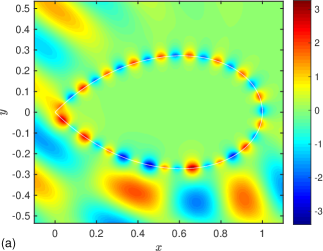
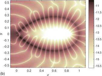
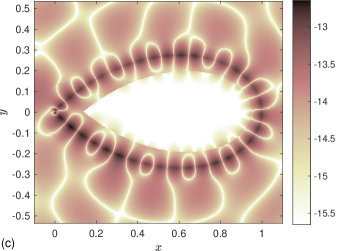
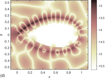
Figure 5: The field $H^{\downarrow}(r,0)$ on the 2D one-corner object with $\varepsilon_{1}=1$, $\varepsilon_{2}=-1.1838$, and $k_{1}=18$: (a) the field $H^{\downarrow}(r,0)$ itself; (b,c,d) $\log_{10}$ of estimated absolute field error using the systems (84), (86), and (87), respectively.

Figure 5(a) shows the total magnetic field $\Re{\rm e}\{H^{\downarrow}(r)\}$, see (2), and Figures 5(b,c,d) show $\log_{10}$ of the estimated absolute error obtained with (84), (86), and (87), respectively. The number of GMRES iterations required to solve the discretized linear systems is 266 for (84), 154 for (86), and 143 for (87). The absolute errors for the systems (84) and (86) are estimated using the solution from (87) as reference.

It is interesting to observe, in Figure 5, that the field accuracy is high for all three systems. The number of digits lost is in agreement with what could be expected for computations on the unit circle, considering the condition numbers shown in Figure 4 and assuming that $k_{1}$ is not close to a true eigenwavenumber. Note also that (87) is a system of Fredholm second-kind integral equations with operator differences that are compact on smooth $\Gamma$ – a property often sought for in integral equation modeling of PDEs. The system (86), on the other hand, contains a Cauchy-type singular difference of operators. Still, the performance of the two systems is very similar.

14.3 Unique solvability on the unit sphere

We repeat the experiment of Section 14.1, but now on the unit sphere using the system (65). Inspired by the good performance of the system (86), reported above and where $\sigma_{\rm E}$ is omitted, we omit both $\sigma_{\rm E}$ and $\sigma_{\rm M}$ from (65) to get a six-scalar-density system. Again, there is noo proof that this system has a unique solution, but every solution to the time harmonic Maxwell’s equations corresponds to a solution to this system.

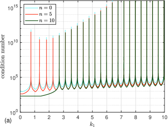
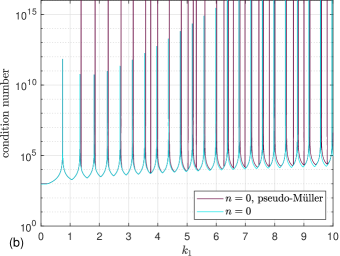
Figure 6: Condition numbers of system matrices on the unit sphere, $\varepsilon_{1}=1$, $\varepsilon_{2}=-1.1838$, and $k_{1}\in[0,10]$: (a) azimuthal modes $n=0,5,10$ of the system (65) with $\sigma_{\rm E}$ and $\sigma_{\rm M}$ omitted; (b) azimuthal mode $n=0$ of the pseudo-Müller system and a repeat of the top curve in (a).

The Fourier–Nyström scheme of [9], see Section 13.2, decomposes the reduced system (65) into a sequence of smaller, modal, systems on the generating curve $\gamma$. Figure 6(a) shows result for the azimuthal modes $n=0,5,10$, with 768 discretization points on $\gamma$, and with approximately $3,\!500$ values of $k_{1}\in[0,10]$. No false eigenwavenumbers can be seen. For comparison, Figure 6(b) shows results for a six-scalar-density variant of the Müller system. The original four-scalar-density Müller system [22, p. 319] uses the surface current densities ${\boldsymbol{M}}_{\rm s}$ and ${\boldsymbol{J}}_{\rm s}$ and contains compact differences of hypersingular operators. These operator differences are hard to implement in three dimensions, even though it definitely is possible on axisymmetric surfaces [18]. Our variant of the Müller system is derived from the original Müller system via integration by parts and relating the surface divergence of ${\boldsymbol{M}}_{\rm s}$ and ${\boldsymbol{J}}_{\rm s}$ to $\varrho_{\rm M}$ and $\varrho_{\rm E}$, see [9, Eqs. (36) and (35)]. This corresponds to omitting both $\sigma_{\rm E}$ and $\sigma_{\rm M}$ from (65) and setting $c_{4}=c_{6}=1$, and $c_{5}=c_{7}=\kappa$. Figure 6(b) shows that this pseudo-Müller system exhibits at least $32$ false eigenwavenumbers for $k_{1}\in[0,10]$.

14.4 Field accuracy for the 3D “tomato”

An incident linearly polarized plane wave with ${\boldsymbol{E}}^{\rm in}({\boldsymbol{r}})=\hat{{\boldsymbol{x}}}e^{{\rm i}k_{1}z}$ and $k_{1}=5$ is scattered against the 3D “tomato” of Section 13.1. The conical point opening angle is $\alpha=31\pi/18$. The same six-scalar-density version of the system (65) is used as in Section 14.3. Only two azimuthal modes, $n=-1$ and $n=1$, are present in this problem and the Fourier coefficients of the surface densities of these modes are either identical or have opposite signs. Therefore only one modal system needs to be solved numerically.

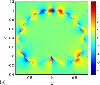
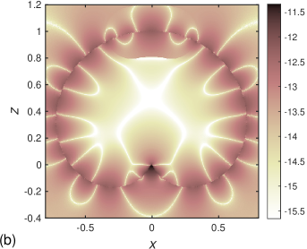
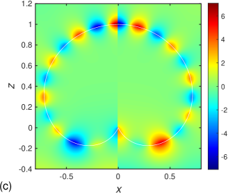
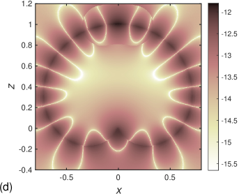
Figure 7: Field images on a cross section of the 3D “tomato” subjected to an incident plane wave ${\boldsymbol{E}}^{\rm in}({\boldsymbol{r}})=\hat{{\boldsymbol{x}}}e^{{\rm i}k_{1}z}$ and with $\varepsilon_{1}=1$, $\varepsilon_{2}=-1.1838$, and $k_{1}=5$: (a) the field $E_{\rho}({\boldsymbol{r}},0)$ with colorbar range set to $[-4.55,4.55]$ ; (b) $\log_{10}$ of estimated absolute field error in $E_{\rho}({\boldsymbol{r}},0)$; (c) the field $H_{\theta}({\boldsymbol{r}},0)$; (d) $\log_{10}$ of estimated absolute field error in $H_{\theta}({\boldsymbol{r}},0)$.

Figure 7 shows the electric field in the $\rho$-direction, $E_{\rho}({\boldsymbol{r}},0)$, and the magnetic field in the $\theta$-direction, $H_{\theta}({\boldsymbol{r}},0)$, on the cross section in Figure 3(c). The results are obtained with $576$ discretization points on the generating curve $\gamma$ and with 242 GMRES iterations. Since the field $E_{\rho}({\boldsymbol{r}},0)$ is singular at the origin, the colorbar range in Figure 7(a) is restricted to the most extreme values of $E_{\rho}({\boldsymbol{r}},0)$ away from the origin. The precision shown in Figure 7(b,d) is consistent with the condition numbers of Figure 6(a) in the sense discussed in Section 14.2. We conclude by noting that Figure 7 clearly shows an accurately computed surface plasmon wave on a non-smooth 3D object in a setup with negative permittivity ratio. To simulate such surface waves is the ultimate goal of this work.

15 Conclusions

A new system of Fredholm second-kind integral equations is presented for an electromagnetic transmission problem involving a single scattering object. Our work can be seen as an extension of the work by Kleinman and Martin [16] on direct methods for scalar transmission problems. Thanks to the introduction of certain uniqueness parameters, our new system gives unique solutions for a wider range of wavenumber combinations than do other systems of integral equations for Maxwell’s equations, for example the original Müller system. In particular, unique solutions are guaranteed for smooth scatterers under the plasmonic condition (1), which is of great interest in physical and engineering applications.

The favorable properties of our new system extend beyond what can be proven rigorously. In a numerical example, a reduced version of the system in combination with a high-order Fourier–Nyström discretization scheme is shown to produce accurate field images of a surface plasmon wave on a non-smooth axisymmetric scatterer.

Appendix

A. Boundary limits of ${\boldsymbol{E}}$ and ${\boldsymbol{H}}$

The relations in Section 2.2 give the following limits at $\Gamma$ for the integral representations of ${\boldsymbol{E}}$ and ${\boldsymbol{H}}$ in (60)–(63):

$$[\nabla\cdot{\boldsymbol{E}}_{1}]^{\pm} =\mp\frac{{\rm i}k_{1}}{2}\sigma_{\rm E}-\frac{{\rm i}k_{1}}{2}\tilde{\cal S}_{k_{1}}\varrho_{\rm E}+\frac{1}{2}\nabla\cdot\tilde{\cal S}_{k_{1}}({\boldsymbol{\nu}}^{\prime}\sigma_{\rm E}+{\boldsymbol{J}}_{\rm s})\,,$$ (A.1)

$${\boldsymbol{\nu}}\cdot{\boldsymbol{E}}_{1}^{\pm} =\pm\frac{1}{2}\varrho_{\rm E}-\frac{1}{2}{\boldsymbol{\nu}}\cdot\boldsymbol{\cal N}_{k_{1}}\varrho_{\rm E}-\frac{1}{2}{\boldsymbol{\nu}}\cdot{\cal R}_{k_{1}}({\boldsymbol{\nu}}^{\prime}\sigma_{\rm M}+{\boldsymbol{M}}_{\rm s})$$

$$\qquad\qquad+\frac{1}{2}{\boldsymbol{\nu}}\cdot\tilde{\cal S}_{k_{1}}({\boldsymbol{\nu}}^{\prime}\sigma_{\rm E}+{\boldsymbol{J}}_{\rm s})+{\boldsymbol{\nu}}\cdot{\boldsymbol{E}}^{\rm in},$$ (A.2)

$${\boldsymbol{\nu}}\times{\boldsymbol{E}}_{1}^{\pm} =\mp\frac{1}{2}{\boldsymbol{M}}_{\rm s}-\frac{1}{2}{\boldsymbol{\nu}}\times\boldsymbol{\cal N}_{k_{1}}\varrho_{\rm E}-\frac{1}{2}{\boldsymbol{\nu}}\times{\cal R}_{k_{1}}({\boldsymbol{\nu}}^{\prime}\sigma_{\rm M}+{\boldsymbol{M}}_{\rm s})$$

$$\qquad\qquad+\frac{1}{2}{\boldsymbol{\nu}}\times\tilde{\cal S}_{k_{1}}({\boldsymbol{\nu}}^{\prime}\sigma_{\rm E}+{\boldsymbol{J}}_{\rm s})+{\boldsymbol{\nu}}\times{\boldsymbol{E}}^{\rm in},$$ (A.3)

$${\boldsymbol{\nu}}\times{\boldsymbol{H}}_{1}^{\pm} =\pm\frac{1}{2}{\boldsymbol{J}}_{\rm s}+\frac{1}{2}{\boldsymbol{\nu}}\times\tilde{\cal S}_{k_{1}}({\boldsymbol{\nu}}^{\prime}\sigma_{\rm M}+{\boldsymbol{M}}_{\rm s})+\frac{1}{2}{\boldsymbol{\nu}}\times{\cal R}_{k_{1}}({\boldsymbol{\nu}}^{\prime}\sigma_{\rm E}+{\boldsymbol{J}}_{\rm s})$$

$$\qquad\qquad-\frac{1}{2}{\boldsymbol{\nu}}\times\boldsymbol{\cal N}_{k_{1}}\varrho_{\rm M}+{\boldsymbol{\nu}}\times{\boldsymbol{H}}^{\rm in},$$ (A.4)

$${\boldsymbol{\nu}}\cdot{\boldsymbol{H}}_{1}^{\pm} =\pm\frac{1}{2}\varrho_{\rm M}+\frac{1}{2}{\boldsymbol{\nu}}\cdot\tilde{\cal S}_{k_{1}}({\boldsymbol{\nu}}^{\prime}\sigma_{\rm M}+{\boldsymbol{M}}_{\rm s})+\frac{1}{2}{\boldsymbol{\nu}}\cdot{\cal R}_{k_{1}}({\boldsymbol{\nu}}^{\prime}\sigma_{\rm E}+{\boldsymbol{J}}_{\rm s})$$

$$\qquad\qquad-\frac{1}{2}{\boldsymbol{\nu}}\cdot\boldsymbol{\cal N}_{k_{1}}\varrho_{\rm M}+{\boldsymbol{\nu}}\cdot{\boldsymbol{H}}^{\rm in},$$ (A.5)

$$[\nabla\cdot{\boldsymbol{H}}_{1}]^{\pm} =\mp\frac{{\rm i}k_{1}}{2}\sigma_{\rm M}+\frac{1}{2}\nabla\cdot\tilde{\cal S}_{k_{1}}({\boldsymbol{\nu}}^{\prime}\sigma_{\rm M}+{\boldsymbol{M}}_{\rm s})-\frac{{\rm i}k_{1}}{2}\tilde{\cal S}_{k_{1}}\varrho_{M}\,,$$ (A.6)

$$[\nabla\cdot{\boldsymbol{E}}_{2}]^{\pm} =\pm\frac{{\rm i}k_{1}}{2\kappa}\sigma_{\rm E}+\frac{{\rm i}k_{1}}{2}\tilde{\cal S}_{k_{2}}\varrho_{\rm E}-\frac{1}{2}\nabla\cdot\tilde{\cal S}_{k_{2}}(\kappa^{-1}{\boldsymbol{\nu}}^{\prime}\sigma_{\rm E}+{\boldsymbol{J}}_{\rm s})\,,$$ (A.7)

$${\boldsymbol{\nu}}\cdot{\boldsymbol{E}}_{2}^{\pm} =\mp\frac{1}{2\kappa}\varrho_{\rm E}+\frac{1}{2\kappa}{\boldsymbol{\nu}}\cdot\boldsymbol{\cal N}_{k_{2}}\varrho_{\rm E}+\frac{1}{2\kappa}{\boldsymbol{\nu}}\cdot{\cal R}_{k_{2}}({\boldsymbol{\nu}}^{\prime}\sigma_{\rm M}+\kappa{\boldsymbol{M}}_{\rm s})$$

$$\qquad\qquad-\frac{1}{2}{\boldsymbol{\nu}}\cdot\tilde{\cal S}_{k_{2}}(\kappa^{-1}{\boldsymbol{\nu}}^{\prime}\sigma_{\rm E}+{\boldsymbol{J}}_{\rm s})\,,$$ (A.8)

$${\boldsymbol{\nu}}\times{\boldsymbol{E}}_{2}^{\pm} =\pm\frac{1}{2}{\boldsymbol{M}}_{\rm s}+\frac{1}{2\kappa}{\boldsymbol{\nu}}\times\boldsymbol{\cal N}_{k_{2}}\varrho_{\rm E}+\frac{1}{2\kappa}{\boldsymbol{\nu}}\times{\cal R}_{k_{2}}({\boldsymbol{\nu}}^{\prime}\sigma_{\rm M}+\kappa{\boldsymbol{M}}_{\rm s})$$

$$\qquad\qquad-\frac{1}{2}{\boldsymbol{\nu}}\times\tilde{\cal S}_{k_{2}}(\kappa^{-1}{\boldsymbol{\nu}}^{\prime}\sigma_{\rm E}+{\boldsymbol{J}}_{\rm s})\,,$$ (A.9)

$${\boldsymbol{\nu}}\times{\boldsymbol{H}}_{2}^{\pm} =\mp\frac{1}{2}{\boldsymbol{J}}_{\rm s}-\frac{1}{2}{\boldsymbol{\nu}}\times\tilde{\cal S}_{k_{2}}({\boldsymbol{\nu}}^{\prime}\sigma_{\rm M}+\kappa{\boldsymbol{M}}_{\rm s})$$

$$\qquad-\frac{1}{2}{\boldsymbol{\nu}}\times{\cal R}_{k_{2}}(\kappa^{-1}{\boldsymbol{\nu}}^{\prime}\sigma_{\rm E}+{\boldsymbol{J}}_{\rm s})+\frac{1}{2}{\boldsymbol{\nu}}\times\boldsymbol{\cal N}_{k_{2}}\varrho_{\rm M}\,,$$ (A.10)

$${\boldsymbol{\nu}}\cdot{\boldsymbol{H}}_{2}^{\pm} =\mp\frac{1}{2}\varrho_{\rm M}-\frac{1}{2}{\boldsymbol{\nu}}\cdot\tilde{\cal S}_{k_{2}}({\boldsymbol{\nu}}^{\prime}\sigma_{\rm M}+\kappa{\boldsymbol{M}}_{\rm s})$$

$$\qquad-\frac{1}{2}{\boldsymbol{\nu}}\cdot{\cal R}_{k_{2}}(\kappa^{-1}{\boldsymbol{\nu}}^{\prime}\sigma_{\rm E}+{\boldsymbol{J}}_{\rm s})+\frac{1}{2}{\boldsymbol{\nu}}\cdot\boldsymbol{\cal N}_{k_{2}}\varrho_{\rm M}\,,$$ (A.11)

$$[\nabla\cdot{\boldsymbol{H}}_{2}]^{\pm} =\pm\frac{{\rm i}k_{1}}{2}\sigma_{\rm M}-\frac{1}{2}\nabla\cdot\tilde{\cal S}_{k_{2}}({\boldsymbol{\nu}}^{\prime}\sigma_{\rm M}+\kappa{\boldsymbol{M}}_{\rm s})+\frac{{\rm i}k_{1}}{2}\kappa\tilde{\cal S}_{k_{2}}\varrho_{M}\,.$$ (A.12)

B. Divergence conditions

The derivations of the conditions for (69), (70), and (78) to hold are all very similar. For this reason we only present a detailed derivation of the condition for (70) to hold.

The fields ${\boldsymbol{E}}_{W}$ and ${\boldsymbol{H}}_{W}$ are defined through (68), (60)–(63), and the solution to (65). Appendix A and (65) give the relations on $\Gamma$

$$\lambda\kappa{\boldsymbol{\nu}}\times{\boldsymbol{E}}_{W}^{+} ={\boldsymbol{\nu}}\times{\boldsymbol{E}}_{W}^{-}\,,$$ (B.1)

$$\lambda\kappa{\boldsymbol{\nu}}\cdot{\boldsymbol{H}}_{W}^{+} ={\boldsymbol{\nu}}\cdot{\boldsymbol{H}}_{W}^{-}\,,$$ (B.2)

$$\gamma_{\rm M}[\nabla\cdot{\boldsymbol{H}}_{W}]^{+} =[\nabla\cdot{\boldsymbol{H}}_{W}]^{-}\,.$$ (B.3)

By combining the surface divergence of (B.1) with (B.2) we get

$$\lambda\kappa({\rm i}k_{1}{\boldsymbol{\nu}}\cdot{\boldsymbol{H}}_{2}^{+}-{\boldsymbol{\nu}}\cdot[\nabla\times{\boldsymbol{E}}_{2})]^{+})={\rm i}k_{1}{\boldsymbol{\nu}}\cdot{\boldsymbol{H}}_{1}^{-}-{\boldsymbol{\nu}}\cdot[\nabla\times{\boldsymbol{E}}_{1})]^{-}\,,$$ (B.4)

where we have used ${\boldsymbol{\nu}}\cdot(\nabla\times{\boldsymbol{\nu}}\times({\boldsymbol{\nu}}\times{\boldsymbol{E}}_{i}))=-{\boldsymbol{\nu}}\cdot(\nabla\times{\boldsymbol{E}}_{i})$, $i=1,2$. By (60)–(63) and limits in Appendix A this leads to

$$\lambda\kappa\left(\kappa^{-1}{\boldsymbol{\nu}}\cdot[\nabla(\nabla\cdot{\cal S}_{k_{2}})]^{+}({\boldsymbol{\nu}}^{\prime}\sigma_{\rm M}+\kappa{\boldsymbol{M}}_{\rm s})-{\rm i}k_{1}{\boldsymbol{\nu}}\cdot\boldsymbol{\cal N}_{k_{2}}\varrho_{\rm M}+{\rm i}k_{1}\varrho_{\rm M}\right)\\ =-{\boldsymbol{\nu}}\cdot[\nabla(\nabla\cdot{\cal S}_{k_{1}})]^{-}({\boldsymbol{\nu}}^{\prime}\sigma_{\rm M}+{\boldsymbol{M}}_{\rm s})+{\rm i}k_{1}{\boldsymbol{\nu}}\cdot\boldsymbol{\cal N}_{k_{1}}\varrho_{\rm M}+{\rm i}k_{1}\varrho_{\rm M}\,.$$ (B.5)

A comparison of (B.5) with the limits ${\boldsymbol{\nu}}\cdot[\nabla(\nabla\cdot{\boldsymbol{H}}_{1})]^{-}$ and ${\boldsymbol{\nu}}\cdot[\nabla(\nabla\cdot{\boldsymbol{H}}_{2})]^{+}$ gives

$$\lambda{\boldsymbol{\nu}}\cdot[\nabla(\nabla\cdot{\boldsymbol{H}}_{2})]^{+}={\boldsymbol{\nu}}\cdot[\nabla(\nabla\cdot{\boldsymbol{H}}_{1})]^{-}\,.$$ (B.6)

Let $\psi_{W}=\nabla\cdot{\boldsymbol{H}}_{W}$, with ${\boldsymbol{H}}_{W}$ from (68). The fundamental solution (3) and the boundary conditions (B.3) and (B.6) make $\psi_{W}$ satisfy

$$\left\{\begin{array}[]{ll}\Delta\psi_{W}({\boldsymbol{r}})+k_{2}^{2}\psi_{W}({\boldsymbol{r}})=0\,,&{\boldsymbol{r}}\in\Omega_{1}\,,\\ \Delta\psi_{W}({\boldsymbol{r}})+k_{1}^{2}\psi_{W}({\boldsymbol{r}})=0\,,&{\boldsymbol{r}}\in\Omega_{2}\,,\\ \gamma_{\rm M}\psi_{W}^{+}({\boldsymbol{r}})=\psi_{W}^{-}({\boldsymbol{r}})\,,&{\boldsymbol{r}}\in\Gamma\,,\\ \lambda{\boldsymbol{\nu}}\cdot[\nabla\psi_{W}]^{+}({\boldsymbol{r}})={\boldsymbol{\nu}}\cdot[\nabla\psi_{W}]^{-}({\boldsymbol{r}})\,,&{\boldsymbol{r}}\in\Gamma\,,\\ \left(\partial_{\hat{{\boldsymbol{r}}}}-{\rm i}k_{2}\right)\psi_{W}({\boldsymbol{r}})=o\left(|{\boldsymbol{r}}|^{-1}\right)\,,&|{\boldsymbol{r}}|\to\infty\,.\end{array}\right.$$ (B.7)

By rescaling $\psi_{W}$ in $\Omega_{1}$, problem (B.7) becomes identical to problem ${\sf B}_{0}$ with $\alpha=\lambda\bar{\gamma}_{\rm M}/|{\gamma}_{\rm M}|^{2}$. Thus if $\{k_{1},k_{2},\alpha=\lambda\bar{\gamma}_{\rm M}\}$ is such that the conditions of Proposition 3.3 hold, then (B.7) only has the trivial solution $\nabla\cdot{\boldsymbol{H}}_{W}=0$ for ${\boldsymbol{r}}\in\Omega_{1}\cup\Omega_{2}$.

The condition for $\nabla\cdot{\boldsymbol{E}}_{W}=0$ is that the set $\{k_{1},k_{2},\alpha=\bar{\gamma}_{\rm E}\bar{\kappa}\}$ is such that the conditions of Proposition 3.3 hold. The condition for (78) to hold is that $({\rm{Arg}}(k_{1}),{\rm{Arg}}(k_{2}))$ is in the set of points of Figure 2(a).

C. Fulfillment of Maxwell’s equations

We show that ${\boldsymbol{E}}$ and ${\boldsymbol{H}}$ of (64) satisfy (50) and that ${\boldsymbol{E}}_{W}$ and ${\boldsymbol{H}}_{W}$ of (68) satisfy (56) if $\nabla\cdot{\boldsymbol{E}}_{i}({\boldsymbol{r}})=\nabla\cdot{\boldsymbol{H}}_{i}({\boldsymbol{r}})=0$, $i=1,2$, and ${\boldsymbol{r}}\in\Omega_{1}\cup\Omega_{2}$.

The rotation of (62) and (63) can be written

$$\nabla\times{\boldsymbol{H}}_{1}({\boldsymbol{r}}) =\frac{{\rm i}k_{1}}{2}{\cal R}_{k_{1}}({\boldsymbol{\nu}}^{\prime}\sigma_{\rm M}+{\boldsymbol{M}}_{\rm s})({\boldsymbol{r}})-\frac{{\rm i}k_{1}}{2}\tilde{\cal S}_{k_{1}}({\boldsymbol{\nu}}^{\prime}\sigma_{\rm E}+{\boldsymbol{J}}_{\rm s})({\boldsymbol{r}})$$

$$+\frac{1}{2}\nabla (\nabla\cdot{\cal S}_{k_{1}}({\boldsymbol{\nu}}^{\prime}\sigma_{\rm E}+{\boldsymbol{J}}_{\rm s}))({\boldsymbol{r}})+\nabla\times{\boldsymbol{H}}^{\rm in}({\boldsymbol{r}})\,,\quad{\boldsymbol{r}}\in\Omega_{1}\cup\Omega_{2}\,,$$ (C.1)

$$\nabla\times{\boldsymbol{H}}_{2}({\boldsymbol{r}}) =-\frac{{\rm i}k_{1}}{2}{\cal R}_{k_{2}}({\boldsymbol{\nu}}^{\prime}\sigma_{\rm M}+\kappa{\boldsymbol{M}}_{\rm s})({\boldsymbol{r}})+\frac{{\rm i}k_{1}}{2}\tilde{\cal S}_{k_{2}}({\boldsymbol{\nu}}^{\prime}\sigma_{\rm E}+\kappa{\boldsymbol{J}}_{\rm s})({\boldsymbol{r}})$$

$$-\frac{1}{2}\nabla(\nabla\cdot{\cal S}_{k_{2}}(\kappa^{-1}{\boldsymbol{\nu}}^{\prime}\sigma_{\rm E}+{\boldsymbol{J}}_{\rm s}))({\boldsymbol{r}})\,,\quad{\boldsymbol{r}}\in\Omega_{1}\cup\Omega_{2}\,.$$ (C.2)

If $\nabla\cdot{\boldsymbol{E}}_{i}=0$, $i=1,2$, it follows from (60) and (61) that

$$\tilde{\cal S}_{k_{1}}\varrho_{\rm E}({\boldsymbol{r}})-\nabla\cdot{\cal S}_{k_{1}}({\boldsymbol{\nu}}^{\prime}\sigma_{\rm E}+{\boldsymbol{J}}_{\rm s})({\boldsymbol{r}}) =0\,,\quad{\boldsymbol{r}}\in\Omega_{1}\cup\Omega_{2}\,,$$ (C.3)

$$\tilde{\cal S}_{k_{2}}\varrho_{\rm E}({\boldsymbol{r}})-\nabla\cdot{\cal S}_{k_{2}}(\kappa^{-1}{\boldsymbol{\nu}}^{\prime}\sigma_{\rm E}+{\boldsymbol{J}}_{\rm s})({\boldsymbol{r}}) =0\,,\quad{\boldsymbol{r}}\in\Omega_{1}\cup\Omega_{2}\,.$$ (C.4)

The Ampère law

$$\begin{split}\nabla\times{\boldsymbol{H}}_{1}({\boldsymbol{r}})&=-{\rm i}k_{1}{\boldsymbol{E}}_{1}({\boldsymbol{r}})\,,\quad{\boldsymbol{r}}\in\Omega_{1}\cup\Omega_{2}\,,\\ \nabla\times{\boldsymbol{H}}_{2}({\boldsymbol{r}})&=-{\rm i}k_{1}\kappa{\boldsymbol{E}}_{2}({\boldsymbol{r}})\,,\quad{\boldsymbol{r}}\in\Omega_{1}\cup\Omega_{2}\,,\end{split}$$ (C.5)

now follows by combining (C.1) and (C.3) with (60), and by combining (C.2) and (C.4) with (61). The Faraday law

$$\nabla\times{\boldsymbol{E}}_{i}({\boldsymbol{r}})={\rm i}k_{1}{\boldsymbol{H}}_{i}({\boldsymbol{r}})\,,\quad i=1,2\,,\quad{\boldsymbol{r}}\in\Omega_{1}\cup\Omega_{2}\,,$$ (C.6)

follows in the same manner from $\nabla\cdot{\boldsymbol{H}}_{i}=0$, $i=1,2$, and by combining the rotation of (60) with (62) and the rotation of (61) with (63). From (C.5) and (C.6) it follows that ${\boldsymbol{E}}$ and ${\boldsymbol{H}}$ of (64) satisfy (50) and that ${\boldsymbol{E}}_{W}$ and ${\boldsymbol{H}}_{W}$ of (68) satisfy (56).

D. Uniqueness for problems C, ${\sf C}_{0}$, and ${\sf D}_{0}$

We sketch a proof that problem ${\sf C}_{0}$ has only the trivial solution and that problem C has at most one solution by relating these problems to problem ${\sf A}_{0}$ and A. We also justify that the criteria for problem ${\sf D}_{0}$ to only have the trivial solution are the same as the criteria in Proposition 3.3 that make problem ${\sf B}_{0}$ only have the trivial solution.

Let $S_{R}$ be a sphere of radius $R$ with outward unit normal ${\boldsymbol{n}}$. Assume that $S_{R}$ is sufficiently large to contain $\Gamma$ and let $\Omega_{1,R}=\{{\boldsymbol{r}}\in\Omega_{1}:|{\boldsymbol{r}}|<R\}$. From Gauss’ theorem we obtain energy relations for problem ${\sf A}_{0}$ and problem ${\sf C}_{0}$

$$\int_{S_{R}}(U\nabla\bar{U})\cdot{\boldsymbol{n}}\,{\rm d}S=\int_{\Omega_{1,R}}\left(|\nabla U|^{2}-\bar{k}_{1}^{2}|U|^{2}\right){\rm d}v+\int_{\Omega_{2}}\left(\bar{\kappa}^{-1}|\nabla U|^{2}-\bar{k}_{1}^{2}|U|^{2}\right){\rm d}v\,,$$ (D.1)

$$-{\rm i}\bar{k}_{1}\int_{S_{R}}(\bar{{\boldsymbol{E}}}\times{{\boldsymbol{H}}})\cdot{\boldsymbol{n}}\,{\rm d}S=\int_{\Omega_{1,R}}\left(|k_{1}|^{2}|{\boldsymbol{E}}|^{2}-\bar{k}_{1}^{2}|{\boldsymbol{H}}|^{2}\right){\rm d}v\\ +\int_{\Omega_{2}}\left(|k_{1}\kappa|^{2}\bar{\kappa}^{-1}|{\boldsymbol{E}}|^{2}-\bar{k}_{1}^{2}|{\boldsymbol{H}}|^{2}\right){\rm d}v\,.$$ (D.2)

The right hand sides of (D.1) and (D.2) are equivalent. By using techniques similar to those in [16, pp. 309–310] and [17, p. 1434] it follows that when $({\rm{Arg}}(k_{1}),{\rm{Arg}}(k_{2}))$ is in the set of points of Figure 2(a), then $U=0$ and ${\boldsymbol{E}}={\boldsymbol{H}}={\boldsymbol{0}}$ in $\Omega_{1}\cup\Omega_{2}$. Standard arguments give that problem C has at most one solution when problem ${\sf C}_{0}$ only has the trivial solution.

In the same manner as above the energy relation for problem ${\sf D}_{0}$ is shown to be equivalent to the energy relation for problem ${\sf B}_{0}$. We can again use [16, pp. 309–310] and [17, p. 1434] to find the criteria that lead to $W=0$ and ${\boldsymbol{H}}_{W}={\boldsymbol{E}}_{W}={\boldsymbol{0}}$. These are the criteria for the set $\{k_{1},k_{2},\alpha=\lambda\}$ in Proposition 3.3.

References

- [1] A. Axelsson, “Transmission problems for Maxwell’s equations with weakly Lipschitz interfaces”, Math. Methods Appl. Sci., 29, 665–714 (2006).
- [2] A.-S. Bonnet-Ben Dhia and C. Carvalho and L. Chesnel and P. Ciarlet, “On the use of perfectly matched layers at corners for scattering problems with sign-changing coefficients”, J. Comput. Phys., 322, 224–247 (2016).
- [3] D. Colton and R. Kress, Integral equation methods in scattering theory, John Wiley & Sons Inc., New York, 1983.
- [4] D. Colton and R. Kress, Inverse acoustic and electromagnetic scattering theory, 2nd ed., Appl. Math. Sci., vol. 93, Springer-Verlag, Berlin, 1998.
- [5] C. L. Epstein, L. Greengard, and M. O’Neil, “Debye sources and the numerical solution of the time harmonic Maxwell equations II”, Comm. Pure Appl. Math., 66, 753–789 (2013).
- [6] C. L. Epstein, L. Greengard, and M. O’Neil, “A high-order wideband direct solver for electromagnetic scattering from bodies of revolution”, J. Comput. Phys., 387, 205–229 (2019).
- [7] J. Helsing, “Integral equation methods for elliptic problems with boundary conditions of mixed type”, J. Comput. Phys., 228, 8892–8907 (2009).
- [8] J. Helsing, “Solving integral equations on piecewise smooth boundaries using the RCIP method: a tutorial”, arXiv:1207.6737v9 [physics.comp-ph] (revised 2018).
- [9] J. Helsing and A. Karlsson, “Resonances in axially symmetric dielectric objects”, IEEE Trans. Microw. Theory Tech., 65, 2214–2227 (2017).
- [10] J. Helsing and A. Karlsson, “On a Helmholtz transmission problem in planar domains with corners”, J. Comput. Phys., 371, 315–332 (2018).
- [11] J. Helsing and A. Karlsson, “Physical-density integral equation methods for scattering from multi-dielectric cylinders”, J. Comput. Phys., 387, 14–29 (2019).
- [12] J. Helsing and K.-M. Perfekt, “The spectra of harmonic layer potential operators on domains with rotationally symmetric conical points”, J. Math. Pures Appl., 118, 235–287 (2018).
- [13] J. Helsing and A. Rosén, “Dirac integral equations for dielectric and plasmonic scattering”, arXiv:1911.00788 [math.AP] (2019).
- [14] J. Homola, “Surface plasmon resonance sensors for detection of chemical and biological species”, Chem. Rev., 108, 462–493 (2008).
- [15] A. Kirsch and F. Hettlich, The mathematical theory of time-harmonic Maxwell’s equations, Appl. Math. Sci., vol. 190, Springer, Cham, 2015.
- [16] R.E. Kleinman and P.A. Martin, “On single integral equations for the transmission problem of acoustics”, SIAM J. Appl. Math., 48, 307–325 (1988).
- [17] R. Kress and G.F. Roach. “Transmission problems for the Helmholtz equation”, J. Math. Phys., 19, 1433–1437 (1978).
- [18] J. Lai and M. O’Neil, “An FFT-accelerated direct solver for electromagnetic scattering from penetrable axisymmetric objects”, J. Comput. Phys., 390, 152–174 (2019).
- [19] J. Li, X. Fu, and B. Shanker, “Decoupled potential integral equations for electromagnetic scattering from dielectric objects”, IEEE Trans. Antennas Propag., 67, 1729–1739 (2018).
- [20] X. Luo, D. Tsai, M. Gu, and M. Hong, “Extraordinary optical fields in nanostructures: from sub-diffraction-limited optics to sensing and energy conversion” Chem. Soc. Rev., 48, 2458–2494 (2019).
- [21] J.R. Mautz and R.F. Harrington. “Electromagnetic scattering from a homogeneous body of revolution”, Tech. Rep. TR-77-10, Dept. of electrical and computer engineering, Syracuse Univ., New York, (1977).
- [22] C. Müller, Foundations of the Mathematical Theory of Electromagnetic Waves. Berlin, Springer-Verlag, 1969.
- [23] H. Raether, Surface plasmons on smooth and rough surfaces and on gratings, vol. 111 of Springer tracts in modern physics, Springer, Berlin, 1988.
- [24] M. Taskinen and P. Ylä-Oijala, “Current and charge integral equation formulation”, IEEE Trans. Antennas Propag., 54, 58–67 (2006).
- [25] D. Tzarouchis and A. Sihvola, “Light scattering by a dielectric sphere: perspectives on the Mie resonances”, Appl. Sci., 8, Article no. 184 (2018).
- [26] F. Vico, M. Ferrando-Bataller, T. Jiménez, and D. Sánchez-Escuderos, “A non-resonant single source augmented integral equation for the scattering problem of homogeneous lossless dielectrics”, 2016 IEEE Int. Symp. Antennas Propag. (APSURSI), 745–746 (2016).
- [27] F. Vico, L. Greengard, and M. Ferrando. “Decoupled field integral equations for electromagnetic scattering from homogeneous penetrable obstacles”, Comm. Part. Differ. Equat. 43, 159–184 (2018).
- [28] P. Young, S. Hao, and P.G. Martinsson, “A high-order Nyström discretization scheme for boundary integral equations defined on rotationally symmetric surfaces”, J. Comput. Phys., 231, 4142–4159 (2012).