Unhiding a concealed resonance by multiple Kondo transitions in a quantum dot

Abstract

Kondo correlations are responsible for the emergence of a zero-bias peak in the low temperature differential conductance of Coulomb blockaded quantum dots. In the presence of a global SU(2)$\otimes$SU(2) symmetry, which can be realized in carbon nanotubes, they also inhibit inelastic transitions which preserve the Kramers pseudospins associated to the symmetry. We report on magnetotransport experiments on a Kondo correlated carbon nanotube where resonant features at the bias corresponding to the pseudospin-preserving transitions are observed. We attribute this effect to a simultaneous enhancement of pseudospin-non-preserving transitions occurring at that bias. This process is boosted by asymmetric tunneling couplings of the two Kramers doublets to the leads and by asymmetries in the potential drops at the leads. Hence, the present work discloses a fundamental microscopic mechanisms ruling transport in Kondo systems far from equilibrium.

The Kondo effect Kondo (1964) is a quintessential example of strong correlations in a many-body system, stemming from the screening of a localized spin by a Fermi sea of conduction electrons. Quantum dots (QD) in the Coulomb blockade regime, which effectively behave as a spin-1/2 system, provide a simple manifestation of SU(2) Kondo entanglement between the dot spin and the lead conduction electrons, leading to the formation of a many-body spin singlet Goldhaber-Gordon et al. (1998); Cronenwett et al. (1998). The Kondo effect in QDs can also have more exotic realizations, provided that the associated degrees of freedom are conserved during tunneling. A prominent example are carbon nanotube (CNT) QDs where the presence of orbital (valley) and spin degrees of freedom leads to the SU(4) Jarillo-Herrero et al. (2005a); Choi et al. (2005); Makarovski et al. (2007); Anders et al. (2008); Ferrier et al. (2016, 2017) and the SU(2)$\otimes$SU(2) Kondo effects Fang et al. (2008); Cleuziou et al. (2013); Schmid et al. (2015); Niklas et al. (2016). The latter occurs when the valley and spin degeneracy of a CNT longitudinal mode is broken by spin-orbit coupling Galpin et al. (2010) or valley mixing Mantelli et al. (2016), giving rise to two time-reversal protected Kramers doublets separated by an inter-Kramers splitting $\Delta$, as seen in Fig. 1(a). A signature of the SU(2)$\otimes$SU(2) Kondo effect is thus the occurrence of a zero-bias anomaly accompanied by two inelastic peaks, symmetrically located with respect to the central peak, in the differential conductance of a CNT with single electron or single hole occupancy Schmid et al. (2015). Similar features are also seen in our experiment, as shown in Figs. 1(b), (c).

In analogy to the more conventional SU(2) case, a pseudospin can be associated to each Kramers doublet of the CNT and the lead electrons Mantelli et al. (2016). While the central peak accounts for elastic virtual transitions which flip the pseudospin of the CNT electron within the same Kramers doublet (${\cal T}$-transition), the inelastic peaks denote transitions involving one state in the lower and one state in the upper Kramers doublet. One distinguishes between chiral (${C}$) and particle-hole (${P}$) transitions if the two states involve the opposite or the same pseudospin, respectively (see Fig. 2(a)). Strikingly, inelastic transitions of the ${P}$ type are inhibited by effective anti-ferromagnetic exchange (Kondo) correlations between the pseudospins of lead and CNT electrons Lim et al. (2006); Mantelli et al. (2016), as confirmed by transport experiments at low magnetic fields Jarillo-Herrero et al. (2005a); Makarovski et al. (2007); Cleuziou et al. (2013); Schmid et al. (2015); Niklas et al. (2016). However, ${P}$-transitions can be observed in the weak coupling regime, where Kondo correlations do not play a role and only lowest order cotunneling processes are responsible for the inelastic peaks Nygård et al. (2000); Jarillo-Herrero et al. (2005b); Jespersen et al. (2011); Niklas et al. (2016).

In this Letter, we demonstrate experimentally the puzzling emergence of a resonance at energies of the inelastic ${P}$-transition in Kondo correlated CNT QDs. Noticeably, the $P$-resonance is clearly seen only for a given bias polarity, suggesting its association with lead coupling asymmetries. We present a comprehensive theoretical analysis based on the Keldysh effective action (KEA) theory Schmid et al. (2015); Smirnov and Grifoni (2013a), addressing the role of asymmetries in Kondo-correlated CNT QDs. The ${P}$-like features arise from the coherent addition of a ${C}$- and a ${\cal T}$-type transition, which occurs when the applied bias equals the energy of the inelastic ${P}$-transition, becoming relevant for different couplings of the Kramers doublets to the leads.

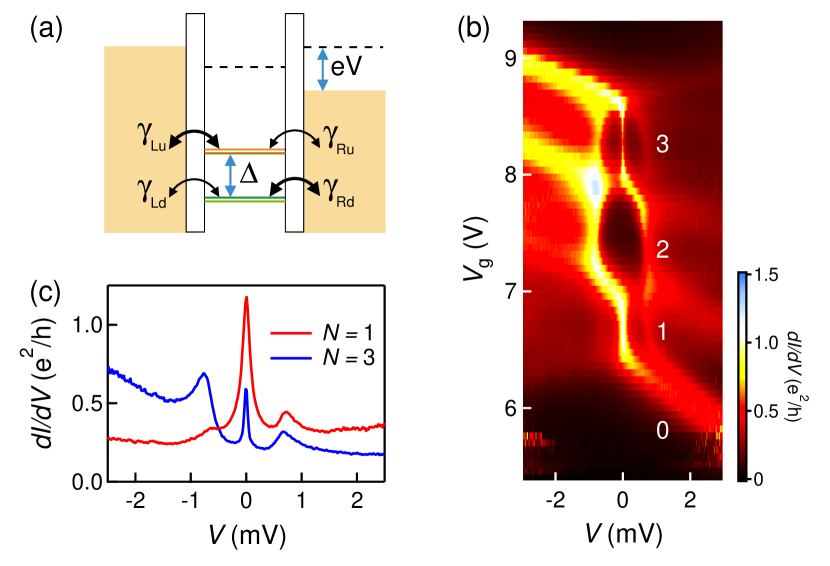
Figure 1: The SU(2)$\otimes$SU(2) Kondo effect. a) A CNT longitudinal shell possesses two Kramers doublets separated by a splitting $\Delta$. The upper (u) and lower (d) doublet are coupled to left (L) and right (R) leads by tunneling couplings $\gamma_{{L}p}$ and $\gamma_{{R}p}$, where $p={\rm u,d}$. b) Experimental differential conductance as a function of gate, $V_{\rm g}$, and bias, $V$, voltages for different occupation of a longitudinal shell. In the valleys with odd occupancy a zero-bias Kondo ridge is clearly seen. Two additional ridges, symmetrically located with respect to the central Kondo peak, are observed at finite bias. The asymmetric response implies the presence of asymmetries in the problem. c) Bias traces taken at gate voltages corresponding to the center of the $N=1$ and $N=3$ valleys show inelastic peaks with roughly the same spacing $\Delta$.

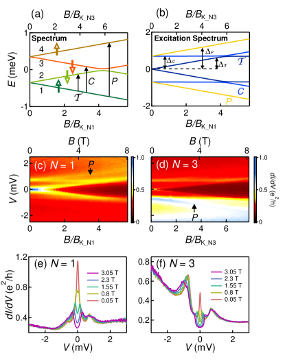
Figure 2: Behavior in perpendicular magnetic field. a) Evolution of energy levels in magnetic field; to each level is associated a Kramers pseudospin. b) Addition spectrum obtained from (a) with inelastic excitations $\Delta_{T},\Delta_{C}$, and $\Delta_{P}$ associated to ${\cal T}$, $C$ and $P$-transitions being indicated. The magnetic field is scaled by the characteristic fields $B_{K_{N1}}=1.425$ T and $B_{K_{N3}}=1.036$ T to emphasize universal behavior. c), d) Experimentally measured differential conductance vs scaled magnetic field. The $P$-like resonances are clearly visible and indicated by an arrow. (e), (f) Experimental $dI/dV$ vs bias voltage for various values of the magnetic field for (e) the one electron and (f) the three electron valley.

Experimental results.- Our device is made of a CNT grown by chemical vapour deposition and connected to Pd($6\ {\rm nm}$)/Al($70\ {\rm nm}$) leads. Fabrication details can be found in Ref. Ferrier et al. (2016). The differential conductance of our CNT QD is shown in Fig. 1(b) as a function of the applied bias $V$ and gate voltage $V_{\rm g}$. A small perpendicular magnetic field $B=0.02$ T is applied to suppress superconductivity of Al in the leads. A Kondo ridge, corresponding to the yellow line at zero bias, is recognized in the Coulomb valleys with occupation $N=1$ and $N=3$ of a longitudinal shell. In the $N=0,2$ valleys, in contrast, no Kondo ridge is seen. Additional inelastic peaks, symmetrically located with respect to zero bias, are observed for the $N=1,2,3$ valleys. Bias traces taken at gate voltages corresponding to the center of a valley are shown in Fig. 1(c). From such traces a Kramers splitting of $\Delta\simeq 0.7$ meV is estimated. Additionally, from the width of the zero-bias peaks Kondo temperatures of $T_{K1}=1$ K and $T_{K3}=0.37$ K are extracted for valley $N=1$ and $N=3$, respectively. Since our experiments are taken at temperatures around $T=30$ mK, it holds $T<T_{K}$. Furthermore, from the evolution in perpendicular magnetic field (see Eq. (2) below), we can extract a spin-orbit coupling splitting $\Delta_{\rm SO}=0.07$ meV and a larger valley mixing energy $\Delta_{{\rm K,K^{\prime}}}=0.7$ meV for both Kondo valleys.

A magnetic field breaks time-reversal symmetry and hence also Kramers degeneracy. The expected evolution of the single particle energy spectrum of a longitudinal shell and its associated excitation spectrum are shown in Figs. 2(a) and (b). The Kondo effect is however a many-body phenomenon, and differences in the excitation spectrum are expected. The experimental magnetoconductance is shown in Figs. 2(c) and (d); the reference field $B_{K}=eV_{K}/\mu_{\rm B}$ is defined through the value $V_{K}$ of the applied bias voltage where the low bias differential conductance $dI/dV$ is $2/3$ of its value at zero-bias. This ensures universal behavior of the scaled magnetoconductance Gaass et al. (2011). Differential conductance traces for different values of the magnetic field are shown in Figs. 2(e) and (f) and characterize the behavior at low fields. We find that the zero bias peak in valley $N=1$ and $N=3$ only splits above a critical field of the order of the reference field $B_{K}$, as expected from theoretical predictions Costi (2000); Smirnov and Grifoni (2013b). Further, the inelastic peaks do not split nor move at small values of the magnetic field for valley $N=1$, suggesting a predominance of inelastic $C$-transitions Schmid et al. (2015); Niklas et al. (2016). Valley $N=3$ can be viewed as a shell with a single hole. Here the side peak at negative bias moves towards larger negative values of the bias voltage as the field increases, suggesting that a $P$-like transition is observed. Hence, the behavior is strongly asymmetric in the bias voltage and the $P$-like resonance is seen only for positive (negative) voltages for electron (hole) transport. In the following we propose a theoretical explanation for the experimental findings.

Model and KEA self-energy.- We consider the four-levels Anderson model to describe a longitudinal mode of a CNT quantum dot with both orbital and spin degrees of freedom. We denote by $|j\rangle$, $j=1,..,4$ the single-particle eigenstates and associate to the lower Kramers doublet the couple (1,2), to the upper the couple (3,4), see Fig. 2(a). The CNT Hamiltonian thus has the form

$$\hat{H}_{\rm CNT}=\sum_{j}\varepsilon_{j}(B)\hat{n}_{j}+\frac{U}{2}\sum_{i\neq j}\hat{n}_{i}\hat{n}_{j}+\hat{H}_{J},$$ (1)

where $\hat{n}_{j}=\hat{d}^{\dagger}_{j}\hat{d_{j}}$ is the occupation operator of level $j$, and $\varepsilon_{1,4}(B)=\varepsilon_{d}\mp\Delta(B)/2$, $\varepsilon_{2,3}(B)=\varepsilon_{1,4}(-B)$. Here

$$\Delta(B) =\sqrt{\Delta_{\mathrm{SO}}^{2}+(\Delta_{\mathrm{K,K^{\prime}}}+g_{s}\mu_{B}B)^{2}}=:\Delta_{P}$$ (2)

is the magnetic field dependent level splitting ($g_{s}\mu_{B}$ is the spin magnetic moment). As indicated in the last equality, such level splitting yields the addition energy for the $P$-resonance. Finally, the second and third terms in Eq. (1) account for charging and exchange effects, respectively. We consider strong electron-electron interactions $(U=\infty)$, such that double occupancy of the impurity is excluded and exchange effects are not relevant. The evolution of the four energy levels $\varepsilon_{j}(B)$ in magnetic field is shown in Fig. 2(a) together with the possible transitions (${\cal T}$, $C,P$) from the ground state. The complete single-particle excitation spectrum is illustrated in Fig. 2(b). Notice that $C$-excitations are independent of the magnetic field until the anticrossing of the inner levels (2,3). Further, it holds the relation $\Delta_{P}=\Delta_{T}+\Delta_{C}$, with $\Delta_{T}=\varepsilon_{2}-\varepsilon_{1}=\varepsilon_{4}-\varepsilon_{3}$, and $\Delta_{C}=\varepsilon_{3}-\varepsilon_{1}=\varepsilon_{4}-\varepsilon_{2}$.

Kondo correlations modify the simple single-particle picture, as shown in Figs. 2(c)-(f). To account for this behavior, we have evaluated the differential conductance of a four-levels Anderson model with bias and tunneling asymmetries using the Keldysh effective action (KEA) method. Assuming that the Kramers degrees of freedom are conserved during tunneling Choi et al. (2005); Lim et al. (2006), KEA yields the tunneling density of states (TDOS) of channel $j$ Schmid et al. (2015)

$$\nu_{j}(\varepsilon,{B})=\frac{\Gamma/2\pi}{[\varepsilon_{j}({B})-\varepsilon+\Gamma_{j}{\rm Re}\Sigma^{\text{}}_{j}(\varepsilon,{B})]^{2}+[\Gamma_{j}{\rm{Im}}\Sigma^{\text{}}_{j}(\varepsilon,{B})]^{2}},$$ (3)

in terms of the KEA self-energies $\Sigma_{j}={\rm{Re}}\Sigma_{j}+i{\rm{Im}}\Sigma_{j}$ being the central quantities of the theory. Here $\Gamma=\sum_{\alpha,j}\Gamma_{\alpha j}/4$ is the average coupling and $\Gamma_{\alpha j}$ are the tunneling couplings of channel $j$ at lead $\alpha=L,R$. The current follows from the Meir and Wingreen formula Meir and Wingreen (1992)

$$I=\frac{e}{\hbar}\sum_{j=1}^{4}\int_{-\infty}^{\infty}d\varepsilon\frac{\Gamma_{Lj}\Gamma_{Rj}}{\Gamma_{Lj}+\Gamma_{Rj}}\nu_{j}(\varepsilon)[f_{L}(\varepsilon)-f_{R}(\varepsilon)],$$ (4)

where $f_{\alpha}=[\exp\beta(\varepsilon-\mu_{\alpha})+1]^{-1}$ is the Fermi function, and $\mu_{L}=\mu_{0}+\eta eV,\mu_{R}=\mu_{0}-(1-\eta)(eV)$ with $\eta\in[0,1]$ accounting for an asymmetric bias drop between the left and right leads. The coupling asymmetry parameter for the lead $\alpha$ and level $j$ is given by $\gamma_{\alpha j}=\Gamma_{\alpha j}/\Gamma_{j}$, with $\Gamma_{j}=\sum_{\alpha}\Gamma_{\alpha j}$. We keep the SU(2) symmetry within the same Kramers channel, and set

$$\gamma_{\alpha 1}=\gamma_{\alpha 2}:=\gamma_{\alpha\rm{d}},\quad\gamma_{\alpha 3}=\gamma_{\alpha 4}:=\gamma_{\alpha\rm{u}},$$ (5)

as illustrated in Fig. 1(a). Such asymmetries enter in the channel self-energies $\Sigma_{j}$, and hence impact the relevance of a given transition. For occupation $N=1$ we find

$$\begin{split}&\Sigma_{j}(\varepsilon,B)=\frac{1}{\pi}\sum_{i=T_{j},C_{j}}\frac{\Gamma_{i}}{\Gamma_{j}}\Bigg{[}\ln\left(\frac{W}{2\pi k_{\rm B}T}\right)+\frac{i\pi}{2}\\ &-\sum_{\alpha}\gamma_{\alpha i}\Psi\left(\frac{1}{2}+\frac{\cal E}{2\pi k_{\rm B}T}-i\frac{\mu_{\alpha}-\varepsilon+\Delta_{ji}}{2\pi k_{\rm B}T}\right)\Bigg{]},\end{split}$$ (6)

where $W$ is a high energy cut-off, $\Psi$ is the digamma function, $\Delta_{ji}=\varepsilon_{j}-\varepsilon_{i}$, and $T_{j},C_{j}$ are the ${\cal T}$- and $C$-partners of level $j$. The case $N=3$ is obtained from Eq. (6) upon replacement of $\Delta_{ji}\to-\Delta_{ji}$. Finally, the complex quantity ${\cal E}$ accounts for low energy contributions which make the self-energy finite also at zero temperature, as discussed in Sec. IV of the Supplemental Material.

Impact of asymmetries.- The analytic forms Eqs. (3), (4) allow us to analyze asymmetry effects on the differential conductance $dI/dV$. Before turning to highly nonequilibrium situations with $eV\simeq\Delta_{P}(B)$, we focus on low energies. An expansion of the zero temperature and zero magnetic field differential conductance $G_{\rm{diff}}$ in powers of the applied bias, $G_{\mathrm{diff}}=G_{0}+G_{1}V+\ldots$, yields

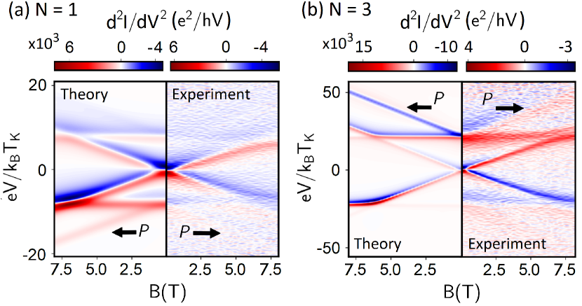
Figure 3: Second derivative of the current, $d^{2}I/dV^{2}$, for the (a) $N=1$ valley and, (b) $N=3$ valley as a function of magnetic field. The left sub-panels show analytical predictions for the asymmetric four-level Anderson model, the right sub-panels the experimental observations. Kondo peaks in the differential conductance are manifested as zeros of $d^{2}I/dV^{2}$ as it changes from positive (red) to negative (blue) with increasing bias. Arrows point to the $P$-resonance.

$$G_{0}=\frac{2e^{2}}{h}\Bigg{[}4\gamma_{L\rm{d}}\gamma_{R\rm{d}}+(\gamma_{L\rm{u}}\gamma_{R\rm{u}}-\gamma_{L\rm{d}}\gamma_{R\rm{d}})\frac{\pi}{2}\Gamma_{\rm u}\nu_{\rm u}(\mu_{0})\Bigg{]},$$ (7)

being independent of the bias asymmetry $\eta$. The second term in the bracket is proportional to the transmission of the upper Kramers doublet at the Fermi level ${\cal T}_{\rm u}(\mu_{0})=\frac{\pi}{2}\Gamma_{\rm u}\nu_{\rm u}(\mu_{0})$, and vanishes in the SU(4) coupling case where $\gamma_{\alpha\rm{u}}=\gamma_{\alpha\rm{d}}=\gamma_{\alpha}$. Then Eq. (7) yields the known Fermi liquid result $G_{0}=4\gamma_{L}\gamma_{R}\frac{2e^{2}}{h}$. The expression for the linear term is lengthier and given in Sec. V of the Supplemental Material. Similar to $G_{0}$, also $G_{1}$ is independent of the bias asymmetry $\eta$. Further, it is finite only in the presence of lead asymmetries encapsulated in the parameter $D_{p}=\gamma_{Lp}-\gamma_{Rp}$, $p={\rm u,d}$. For finite $D_{u}=D_{d}$ and $\Delta=0$ we recover known results for the SU(4) case Mora et al. (2009). Here the linear term $G_{1}$ is non vanishing due to a small shift of the TDOS peak from the Fermi energy, as expected from the Friedel sum rule Hewson (1993). These results show that asymmetries can yield qualitatively different low energy behavior of a SU(2)$\otimes$SU(2) Kondo QD with respect to the symmetric case. Further, they suggest that the strong asymmetric behavior observed in the experimental data of Fig. 2 requires couplings $\gamma_{\alpha\rm{d}}\neq\gamma_{\alpha\rm{u}}$.

Resonances at finite bias.- We start our analysis by showing in Fig. 3 KEA predictions for $d^{2}I/dV^{2}$. The parameters $\Delta_{\rm K,K^{\prime}}$ and $\Delta_{\rm SO}$ are obtained from Eq. (2) by a fit of the experimental magnetoconductance at large enough fields. The total linewidth $\Gamma$ is extracted from a fit of the data near the charge peaks, as explained in the Supplemental Material. We fix $W/\Gamma=100$; the remaining chosen set of free parameters is shown in Table 1.

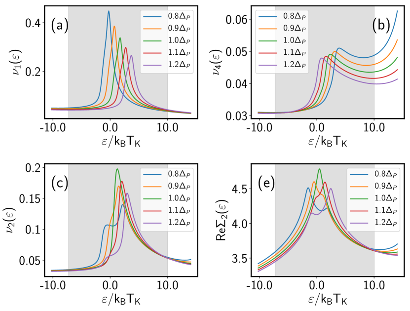
Figure 4: Channel density of states $\nu_{j}$, (a)-(d), and self-energy $\Sigma_{2}$ of channel 2, panels (e) and (f), evaluated at bias drops $eV\simeq\Delta_{P}$, where $\Delta_{P}$ is the addition energy of the $P$-resonance, for the $N=1$ case at $B=8.05T$. The gray stripe indicates the bias window set by the lead chemical potentials when $eV=\Delta_{P}$. At $eV=\Delta_{P}$ the channel density of states $\nu_{2}$ and $\nu_{3}$ are maximal and of the order of $\nu_{1}$. This is due to a resonance of the associated self-energy, as illustrated in (e), (f) on the example of $\Sigma_{2}$. On the other hand $\nu_{4}$ is negligible.

As in the experiment, the KEA current-voltage characteristics display a $P$-peak at negative (positive) potential drop $eV$ for valley $N=1$ ($N=3$).

To understand the origin of the resonance, we analyze each individual TDOS $\nu_{j}$. In general, Kondo resonances appear in the differential conductance when a peak in one or more of the $\nu_{j}(\varepsilon)$ enters the bias window defined by $\mu_{L}-\mu_{R}=eV$. As seen from Eq. (6), the $\nu_{j}$ explicitly and significantly depend on the applied bias voltage through their self-energies $\Sigma_{j}$. Further, peaks in $\nu_{j}$ originate from peaks in Re$\Sigma_{j}$. At low temperatures, the latter occur when $\varepsilon=\mu_{\alpha}+\Delta_{ji}-$Im${\cal E}$, with $i=T_{j},C_{j}$. Simultaneously, Im$\Sigma_{j}$ drops by $\gamma_{{\alpha}i}$ as $\varepsilon$ is swept across the resonance. Conventional Kondo resonances, i.e., the ${\cal T}$- and $C$-resonances, arise as a consequence of a peak in $\nu_{1}$ entering the bias window. The mechanism for the $P$-resonance is different.

In Fig. 4 we focus on the resonance in the $N=1$ valley. We show the energy dependence of each $\nu_{j}(\varepsilon,eV)$ for different potential drops $eV\simeq\Delta(B)=\Delta_{P}$ for a magnetic field $B=8.05T$. The gray region indicates the bias window for asymmetric potential drop $\eta=0.4$ and $eV=\Delta_{P}$. From Figs. 4(a) and (b), we see that $\nu_{1}$ is large while $\nu_{4}$ is negligible in the integration window; further, $\nu_{1}$ exhibits a monotonic variation as the potential drop increases. Strikingly, $\nu_{2}$ and $\nu_{3}$ develop a peak at $eV=\Delta_{P}$ and are of the same order of $\nu_{1}$, as seen in Figs. 4(c) and (d). The peak reflects a resonant feature of $\Sigma_{2}$ and $\Sigma_{3}$, as shown in panels (e) and (f) on the example of $\Sigma_{2}$. This occurs because when $\mu_{L}-\mu_{R}=\Delta_{P}(=\Delta_{C}+\Delta_{T}$) the resonances of $\Sigma_{2}$ ($\Sigma_{3}$) at $\varepsilon=\mu_{R}+\Delta_{T}$ and $\varepsilon=\mu_{L}-\Delta_{C}$ ($\varepsilon=\mu_{R}+\Delta_{C}$ and $\varepsilon=\mu_{L}-\Delta_{T}$) merge into a single concerted resonance. Correspondingly, the differential magnetoconductance displays a small resonance feature also at voltages matching the condition $eV=\Delta_{P}(B)$, as seen in Fig. 3. While the existence of this effect is independent of asymmetries, its magnitude does depend on them. Numerically, for $N=1$ ($N=3$) we find coupling asymmetry thresholds $\zeta_{1}$ ($\zeta_{3}$) above which the resonance is seen. E.g. for the valley $N=1$ and $V<0$ it should hold that $\gamma_{L\rm{u}}-\gamma_{L\rm{d}}>\zeta_{1}$. If the coupling strengths are reverted, $\gamma_{L\rm{d}}-\gamma_{L\rm{u}}>\zeta_{1}$, the resonance occurs at positive rather than at negative bias. Finally, the conditions for the single hole case, $N=3$, can be obtained from the $N=1$ case by replacing ${\rm u}\leftrightarrow\rm{d}$ and $\zeta_{1}$ with $\zeta_{3}$. Thus, if a $P$-resonance is observed at positive bias in the $N=1$ valley, it is likely that such resonance also occurs at negative bias in the $N=3$ valley, in agreement with the experimental observations. Further, bias asymmetry may make it easier to observe a $P$-resonance for small values of $\mu_{0}-\varepsilon_{d}$. The reason for this is that the tails from the charge-transfer peaks may assist the $P$-peaks if they are located at the same bias polarity. Since the asymmetry parameter $\eta$ defines the bias window for the integration variable $\varepsilon\in[\mu_{0}+\eta eV,\mu_{0}-(1-\eta)eV]$, $P$-peaks obtained at $\mu_{L}-\mu_{R}>0$ are assisted by charge-transfer tails for $\eta<0.5$, as seen in Fig. 1 and Fig. 2.

Table 1: Parameters used to fit the experimental data

$N$	$\Gamma$	$\mu_{0}-\varepsilon_{d}$	$\gamma_{L\rm d}$	$\gamma_{L\rm{u}}$	$\eta$
1	3.5 meV	4.83	0.42	0.08	0.42
3	2.4 meV	5.36	0.3	0.06	0.1

Note that virtual processes which involve a direct inelastic transition from the $j=1$ to the $j=4$ channel, namely a $P$-transition, are not explicitly appearing in the KEA self-energies Eq. (6). Pseudospin conserving cotunneling transitions become important at high temperatures and are the dominant contribution to $P$-like resonances outside the Kondo regime Niklas et al. (2016); Jespersen et al. (2011).

Conclusion.- We have observed the emergence of inelastic resonances at bias voltages corresponding to pseudospin conserving $P$-transitions in a Kondo correlated CNT-QD. Due to the antiferromagnetic character of Kondo correlations, which inhibit direct $P$-transitions, these resonances emerge non trivially from a coherent addition of pseudospin non-conserving ${\cal T}$- and $C$- transitions. The here established mechanism for $P$-like resonance becomes prominent in the presence of asymmetries in the tunneling coupling and bias drop.

A.L. and T.H. equally contributed to this work. We acknowledge support by the Deutsche Forschungsgemeinschaft within SFB 689, SFB 1277 B04, and by JSPS KAKENHI Grant Numbers JP15J01518, JP19H00656, and JP19H05826.

References

- Kondo (1964) J. Kondo, Progress of Theoretical Physics 32, 37 (1964).
- Goldhaber-Gordon et al. (1998) D. Goldhaber-Gordon, H. Shtrikman, D. Mahalu, D. Abusch-Magder, U. Meirav, and M. A. Kastner, Nature 391, 156 (1998).
- Cronenwett et al. (1998) S. M. Cronenwett, T. H. Oosterkamp, and L. P. Kouwenhoven, Science 281, 540 (1998).
- Jarillo-Herrero et al. (2005a) P. Jarillo-Herrero, J. Kong, H. S. J. van der Zant, C. Dekker, L. P. Kouwenhoven, and S. De Franceschi, Nature 434, 484 (2005a).
- Choi et al. (2005) M.-S. Choi, R. López, and R. Aguado, Phys. Rev. Lett. 95, 067204 (2005).
- Makarovski et al. (2007) A. Makarovski, J. Liu, and G. Finkelstein, Phys. Rev. Lett. 99, 066801 (2007).
- Anders et al. (2008) F. Anders, D. Logan, M. Galpin, and G. Finkelstein, Phys. Rev. Lett. 100, 086809 (2008).
- Ferrier et al. (2016) M. Ferrier, T. Arakawa, T. Hata, R. Fujiwara, R. Delagrange, R. Weil, R. Deblock, R. Sakano, A. Oguri, and K. Kobayashi, Nature Physics 12, 230 (2016).
- Ferrier et al. (2017) M. Ferrier, T. Arakawa, T. Hata, R. Fujiwara, R. Delagrange, R. Deblock, Y. Teratani, R. Sakano, A. Oguri, and K. Kobayashi, Phys. Rev. Lett. 118, 196803 (2017).
- Fang et al. (2008) T.-F. Fang, W. Zuo, and H.-G. Luo, Phys. Rev. Lett. 101, 246805 (2008).
- Cleuziou et al. (2013) J. P. Cleuziou, N. V. N’Guyen, S. Florens, and W. Wernsdorfer, Phys. Rev. Lett. 111, 136803 (2013).
- Schmid et al. (2015) D. R. Schmid, S. Smirnov, M. Margańska, A. Dirnaichner, P. L. Stiller, M. Grifoni, A. K. Hüttel, and C. Strunk, Phys. Rev. B 91, 155435 (2015).
- Niklas et al. (2016) M. Niklas, S. Smirnov, D. Mantelli, M. Marganska, N.-V. Nguyen, W. Wernsdorfer, J.-P. Cleuziou, and M. Grifoni, Nature Communications 7, 12442 (2016).
- Galpin et al. (2010) M. R. Galpin, F. W. Jayatilaka, D. E. Logan, and F. B. Anders, Phys. Rev. B 81, 075437 (2010).
- Mantelli et al. (2016) D. Mantelli, C. Moca, G. Zaránd, and M. Grifoni, Physica E 77, 180 (2016).
- Lim et al. (2006) J. S. Lim, M.-S. Choi, M. Y. Choi, R. López, and R. Aguado, Phys. Rev. B 74, 205119 (2006).
- Nygård et al. (2000) J. Nygård, D. H. Cobden, and P. E. Lindelof, Nature 408 (2000).
- Jarillo-Herrero et al. (2005b) P. Jarillo-Herrero, J. Kong, H. S. J. van der Zant, C. Dekker, L. P. Kouwenhoven, and S. De Franceschi, Phys. Rev. Lett 94, 156802 (2005b).
- Jespersen et al. (2011) T. Jespersen, K. Grove-Rasmussen, J. Paaske, K. Muraki, J. Nygård, and K. Flensberg, Nature Physics 7, 348 (2011).
- Smirnov and Grifoni (2013a) S. Smirnov and M. Grifoni, Phys. Rev. B 87, 121302 (2013a).
- Gaass et al. (2011) M. Gaass, A. K. Huettel, K. Kang, I. Weymann, J. von Delft, and C. Strunk, Phys. Rev. Lett. 107, 176808 (2011).
- Costi (2000) T. Costi, Phys. Rev. Lett. 85, 1504 (2000).
- Smirnov and Grifoni (2013b) S. Smirnov and M. Grifoni, New J. Phys. 15, 073047 (2013b).
- Meir and Wingreen (1992) Y. Meir and N. Wingreen, Phys. Rev. Lett. 68, 2512 (1992).
- Mora et al. (2009) C. Mora, P. Vitushinsky, X. Leyronas, A. A. Clerk, and K. Le Hur, Phys. Rev. B 80, 155322 (2009).
- Hewson (1993) A. C. Hewson, The Kondo Problem to Heavy Fermions, Cambridge Studies in Magnetism (Cambridge University Press, 1993).