Quantifying the ill-conditioning of analytic continuation

Abstract

Analytic continuation is ill-posed, but becomes merely ill-conditioned (although with an infinite condition number) if it is known that the function in question is bounded in a given region of the complex plane. In an annulus, the Hadamard three-circles theorem implies that the ill-conditioning is not too severe, and we show how this explains the effectiveness of Chebfun and related numerical methods in evaluating analytic functions off the interval of definition. By contrast, we show that analytic continuation is far more ill-conditioned in a strip or a channel, with exponential loss of digits of accuracy at the rate $\exp(-\pi x/2)$ as one moves along. The classical Weierstrass chain-of-disks method loses digits at the faster rate $\exp(-e\kern 0.3ptx)$.

1 Introduction

Analytic continuation is well known to be ill-posed. To be precise, suppose a function $f$ is analytic in a connected open region $\Omega$ of the complex plane and we know its values in a set $E\subset\overline{\Omega}$ to an accuracy of $\varepsilon>0$. (We assume $E$ is a bounded nonempty continuum whose closure does not enclose any points of $\Omega\backslash\overline{E}$, and that $f$ extends analytically to $E$.) This implies no bounds whatsoever on the value of $f$ at any point $z\in\Omega\backslash\overline{E}$ (see Theorem 5.1). And yet if we knew $f$ exactly in $E$, this would determine its values in $\Omega$ exactly.

In practice, nevertheless, analytic continuation from inexact data is carried out all the time, and what makes this possible is regularization, the introduction of additional smoothness assumptions. Often an extrapolation technique is applied without such assumptions being made explicit—and this is understandable, for in applications, often one has a sense of certain features of one’s function without being able to pin them down precisely. In this paper, however, we wish to be completely explicit and show how certain natural regularizing assumptions lead to upper and lower bounds on the accuracy of analytic continuation.

Our regularizing assumption will be that $f$ is not only analytic in $\Omega$, but bounded. For example, we can take the bound to be ${\textstyle{1\over 2}}$ and consider the set of functions that are analytic in $\Omega$ and satisfy $\|f\|_{\Omega}\leq{\textstyle{1\over 2}}$. (The symbol $\|\cdot\|_{A}$ always denotes the supremum norm over the set $A$.) If $f,\tilde{f}$ are two such functions, then $\|\tilde{f}-f\|_{\Omega}\leq 1$. We shall show (Theorem 5.2) that if in addition $\|\tilde{f}-f\|_{E}\leq\varepsilon$, then for each $z\in\Omega\backslash\overline{E}$,

$$|\tilde{f}(z)-f(z)|\leq\varepsilon^{\alpha(z)}$$ (1)

for some $\alpha(z)\in(0,1)$ that depends on $\Omega$, $E$, and $z$ but not on $f$ and $\tilde{f}$ or $\varepsilon$. Another way to say the same thing is

$$\log|\tilde{f}(z)-f(z)|\leq\alpha(z)\log\varepsilon.$$ (2)

We may interpret (2) as follows: if we know a function $f$ satisfying $\|f\|_{\Omega}\leq{\textstyle{1\over 2}}$ to $d$ digits on $E$, then it is determined to $\alpha(z)\kern 0.3ptd$ digits at $z$. Even though our theorems are, of course, mathematical rather than computational results, we shall use the terminology of digits a good deal in discussing them, for this is an easy way to talk about logarithmic quantities.

This general framework may sound rather abstract. It becomes concrete when we consider the dependence of $\alpha(z)$ on $z$ for particular choices of $\Omega$ and $E$, and after stating a basic lemma in Section 2, we shall focus on two choices that are particularly fundamental. The first is radial geometry, with analytic continuation outward from the unit disk $E$ into a disk $\Omega$ of radius $R>1$ (Section 3). In this setting analytic continuation is reasonably well-conditioned, with digits of accuracy being lost only linearly as $|z|$ increases. This observation possibly goes back to Hadamard himself, and its numerical implications have been considered by various authors including Miller miller and Franklin franklin . An intuitive way to understand the effect is to note that in the limiting case $R\to\infty$, Liouville’s theorem implies that $f$ must be constant, so if we know $f$ to accuracy $\varepsilon$ on $E$, we know it to the same accuracy everywhere. The result for finite $R$ (Theorem 3.1) can be derived from the Hadamard three-circles theorem hille . The essence of the matter is that analyticity and boundedness at a large radius imply rapid exponential decrease of Taylor coefficients, hence good behavior at smaller radii.

Analytic continuation is much more difficult in the other geometry we focus on, which is linear (Section 4). Here we take $\Omega$ to be an infinite half-strip of half-width $1$ (without loss of generality), and $E$ as the end segment of the half-strip. As $z$ moves away from $E$ along the centerline of the strip, digits are lost exponentially as a function of distance, and we prove this by reducing the problem to the configuration of Lemma 1. At a point $z$ that is $2\pi$ units away from the end, for example, the number of accurate digits has shrunk by a factor $(\pi/4)\exp(\pi^{2})\approx\hbox{15,000}$, so if you want to have $3$ digits of accuracy at such a point, you’ll need to start with 45,000 digits.

Our formulations are conformally invariant, and thus different regions $\Omega\neq{\bf C}$ can be transplanted from one to another. In particular, analytic continuation in a disk and a half-strip are essentially equivalent problems, and the reason the half-strip is exponentially more difficult than the disk is that the conformal map that relates them is an exponential. Section 5 explores results for general regions (not necessarily simply connected) that follow from these observations, presenting theorems establishing the behavior asserted in the opening paragraphs of this introduction.

Along the way, we shall relate our results to numerical algorithms. Section 3 presents a simple method for numerical analytic continuation in a disk that approximately achieves the bounds indicated in Theorem 3.1, based on Taylor series on the disk, and in Section 6 we show that this method is implicit in Chebfun chebfun ; atap . An algorithm of this kind was proposed by Franklin franklin , and there is recent related work by Demanet and coauthors batenkov ; demtow , among others. Further numerical algorithms and associated mathematical estimates for analytic continuation can be found in cannm ; douglas ; fdfd ; fdfq ; fzcm ; hen66 ; henrici ; miller ; niet ; reichel ; stef ; vessella . More generally, there is a large literature of numerical methods for ill-posed problems, which are often defined by partial differential or integral equations. One paper that speaks of the connection between analytic continuation and more general ill-posed problems defined by PDEs is miller .

In Section 7 we turn to the most famous algorithm of analytic continuation, which goes back to Weierstrass: marching Taylor expansions from one overlapping disk to another in a chain. We show that this method, if carried out numerically in the half-strip with a certain optimal choice of parameters, suffers exponential loss of accuracy at a rate $2\kern 0.3pte/\pi$ times faster than the optimal rate in a half-strip, so that if one marches $2\pi$ units down the half-strip, the number of accurate digits is divided by $\exp(2\pi e)\approx\hbox{26,000,000}$.

Before turning to the details, we comment on the relationship between approximation methods based on multiple derivative values at a single point, such as chain-of-disks continuation of Taylor series or Padé approximation bgm , and methods based just on function values but at multiple points. Our formulations are of the latter form, but the two contexts are close. Thanks to the standard lemma of complex analysis known as Cauchy’s estimate, knowing a function $f$ on the unit disk to accuracy $\varepsilon$ is approximately the same as knowing its Taylor coefficients $c_{k}$ to accuracy $\varepsilon$, and more generally, if $f$ is known to accuracy $\varepsilon$ on the closed disk of radius $r$, this is approximately the same as knowing its Taylor coefficients $c_{k}$ to accuracy $\varepsilon\kern 0.5ptr^{-k}$.

2 A lemma

Our results are based on the following lemma, the Hadamard three-lines theorem, a more general form of which can be found in (rudin, , Thm. 12.8). Numerical algorithms for this geometry are discussed in fdfq .

Lemma 1

Let $h$ be an analytic function in the infinite strip $S=\{w:\,0<\hbox{\kern 0.5pt\rm Re}\kern 1.3ptw<1\}$ with $\|h\|_{S}\leq 1$ and $\lim_{u\downarrow 0}\sup_{v}|h(u+iv)|\leq\varepsilon$ for some $\varepsilon\in(0,1)$. Then for all $w\in S$,

$$\log|h(w)|\leq(1-\hbox{\kern 0.5pt\rm Re}\kern 1.3ptw)\log\varepsilon,\hbox{\quad i.e.,\quad}|h(w)|\leq\varepsilon^{1-\hbox{\kern 0.4pt\scriptsize\rm Re}\kern 1.1ptw}.$$ (3)

Conversely, for any $\varepsilon\in(0,1)$, there is a function $h$ satisfying the given conditions for which the inequalities $(\ref{lemmaeq})$ hold as equalities for all $z$ with $0<\hbox{\kern 0.5pt\rm Re}\kern 1.3ptz<1$.

Proof

We begin by noting that without loss of generality, we may suppose that $h$ is analytic on the closed set $\overline{S}$. If not, we could restrict attention to a smaller domain $\delta\leq\hbox{\kern 0.5pt\rm Re}\kern 1.3ptw\leq 1-\delta$ for $\delta<0$ and then take the limit $\delta\to 0$.

Set $\nu=-\log\varepsilon$, implying $e^{-\nu}=\varepsilon$. The function $e^{-\nu\kern 0.5ptw}h(w)$ is analytic in $\overline{S}$ and bounded in absolute value by $\varepsilon$ for $\hbox{\kern 0.5pt\rm Re}\kern 1.3ptw=0$ and also for $\hbox{\kern 0.5pt\rm Re}\kern 1.3ptw=1$. Therefore, by the maximum modulus principle as qualified in the next paragraph, it is bounded by $\varepsilon$ for all $w\in\overline{S}$. Thus $|h(w)|\leq\varepsilon\kern 0.5pte^{\kern 0.7pt\nu\hbox{\kern 0.4pt\scriptsize\rm Re}\kern 1.1ptw}=e^{(1-\hbox{\kern 0.4pt\scriptsize\rm Re}\kern 1.1ptw)\log\varepsilon}$, as required.

The qualification just mentioned is that the maximum modulus principle does not apply to arbitrary functions on an unbounded domain with a gap in the boundary at $\infty$. However, this function is known to be bounded in an infinite strip, and in such a situation, according to a Phragmén–Lindelöf theorem (hille, , Thm. 18.1.4), the maximum modulus principle applies after all.

For the converse, it is enough to consider the function $h(w)=\varepsilon\kern 0.5pte^{\kern 0.7pt\nu w}$. ∎

3 Analytic continuation in a disk

Figure 1 shows our first fundamental geometry, one that has been considered by a number of authors. We take $E$ to be the closed unit disk and $\Omega$ as the open disk of radius $R>1$. As always, our concern is obtaining bounds on $|\kern 0.3ptg(z)|,$ $z\in\Omega\backslash E$, for an analytic function $g$ ($=\tilde{f}-f\kern 0.7pt$) satisfying $\|\kern 0.3ptg\|_{\Omega}\leq 1$ and $\|\kern 0.3ptg\|_{E}\leq\varepsilon$. Here is the result, essentially the Hadamard three-circles theorem, with $\|\cdot\|_{r}$ denoting the supremum norm over $\{z:\,|z|<r\}$.

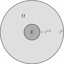
Figure 1: Analytic continuation of a function $f$ from the unit disk $E$ to a larger disk $\Omega$ where it is bounded. If $f$ is known to $d$ digits on $E$, the number of digits determined in $\Omega$ falls off smoothly to $0$ at the outer boundary.

Theorem 3.1

Given $R>1$, let $g$ be analytic in $\Omega=\{z\in{\bf C}:\,|z|<R\}$ with $\|\kern 0.3ptg\|_{R}\leq 1$ and $\|\kern 0.3ptg\|_{1}\leq\varepsilon\in(0,1)$. Then for any $z$ with $1<|z|<R$,

$$\log|\kern 0.3ptg(z)|\leq\alpha(z)\log\varepsilon,\hbox{\quad i.e.,\quad}|\kern 0.3ptg(z)|\leq\varepsilon^{\alpha(z)},$$ (4)

where

$$\alpha(z)=1-{\log|z|\over\log R}.$$ (5)

Conversely, for an infinite sequence of values $\varepsilon$ converging to $0$, there are functions $g$ satisfying the given conditions for which the inequalities $(\ref{ineq1})$ hold as equalities for all $z$ with $1<|z|<R$.

Proof

As in the proof of Lemma 1, we begin by noting that without loss of generality, we may suppose that $g$ is analytic in the closed domain $|z|\leq R$. We transplant the problem to the infinite strip $\overline{S}$ of the last section by defining $h(w)=g(z)$ for $z=R^{\kern 0.8ptw}=e^{w\log R}$, hence $w=\log z/\log R$ (it doesn’t matter which branch of $\log z$ is used, as they all lead to the same estimate). By the lemma, we have $\log|\kern 0.3ptg(z)|\leq(1-\hbox{\kern 0.5pt\rm Re}\kern 1.3ptw)\log\varepsilon=(1-\log|z|/\log R)\log\varepsilon$, as claimed.

For the converse result, consider $g(z)=(z/R)^{n}$ with $n=-\log\varepsilon/\log R$. For an infinite sequence of values $\varepsilon\to 0$, $n$ is an integer, and in these cases $g$ is an analytic function with the required properties. ∎

In words, we can describe Theorem 3.1 as follows. If $f$ is known to $d$ digits for $|z|\leq 1$, the number of digits determined for $|z|=r$ diminishes to $0$ as $r\to R\kern 1.0pt$; as a function of $\log r$, the loss of digits is linear. At $r=\sqrt{R}$, for example, $f$ is determined to $d/2$ digits.

It is easy to outline an algorithm for analytic continuation, based on a finite Taylor series of length $n\approx-\log\varepsilon/\log R$, that achieves approximately the accuracy promised in Theorem 3.1. From approximate values for $|z|=1$ with error at most $\varepsilon$ of a function $f$ with $\|f\|_{\Omega}\leq{\textstyle{1\over 2}}$, we compute approximations $\tilde{c}_{k}\approx c_{k}$ to the Taylor coefficients $\{c_{k}\}$ of $f$ for $0\leq k\leq n$ with $|\tilde{c}_{k}-c_{k}|\leq\varepsilon$. That this is possible follows from Cauchy’s estimate applied on the circle $|z|=1$; in practice, we sample $f$ on a grid of $N\gg n$ roots of unity and use the Fast Fourier Transform akt . By Cauchy’s estimate applied now for $|z|=R$, the Taylor coefficients of $f$ satisfy $|c_{k}|\leq{\textstyle{1\over 2}}R^{-k}$. If we define

$$\tilde{f}(z)=\sum_{k=0}^{n}\tilde{c}_{k}z^{k},$$ (6)

then we have

$$\tilde{f}(z)-f(z)=\sum_{k=0}^{n}(\tilde{c}_{k}-c_{k})z^{k}-\sum_{k=n+1}^{\infty}c_{k}z^{k},$$

implying

$$|\tilde{f}(z)-f(z)|\leq\sum_{k=0}^{n}\varepsilon|z|^{k}+{\textstyle{1\over 2}}\sum_{k=n+1}^{\infty}(|z|/R)^{k}.$$

Our choice $n\approx-\log\varepsilon/\log R$ implies $\varepsilon\approx R^{-n}$, and thus these two sums are both of size on the order of $(|z|/R)^{n}$. We therefore achieve, as required,

$$|\tilde{f}(z)-f(z)|\approx(R/|z|)^{-n}=R^{-\alpha(z)n}\approx\varepsilon^{\alpha(z)},$$

with the equality in the middle holding since the definition (5) implies $R^{\kern 0.8pt\alpha(z)}=R/|z|$.

In the algorithm just described, the regularization occurred when we took the series (6) to be finite rather than infinite. In this geometry, the ill-posedness of analytic continuation resides in the fact that as $k\to\infty$, powers $z^{k}$ have unbounded discrepancies of absolute value between one radius $|z|$ and another. For a fascinating analysis of the implications of such behavior in the context of computation of Taylor coefficients, see born . The importance of truncating a series for numerical analytic continuation was recognized at least as early as lewis , and a detailed error analysis of an algorithm with this flavor can be found in franklin .

We have described the algorithm as a process for working with a function known to accuracy $\varepsilon$ on the unit disk. One way to obtain such data is to take Taylor polynomials of $f$ of successively higher degrees (in exact arithmetic), in which case (4) amounts to the statement that the convergence of Taylor polynomials to $f(z)$ for $|z|<R$ is exponential at a rate of order $(|z|/R)^{n}$.

4 Analytic continuation in a half-strip

Our second fundamental geometry is shown in Figure 2. Now $E$ is the complex interval $(-i,i\kern 0.7pt)$ and $\Omega$ is the half-strip $H$ of points $z=x+iy$ with $x>0$, $-1<y<1$. Our aim is to analytically continue a function $f$ from the end segment of the strip to real positive values $x$.

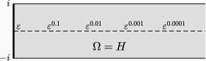
Figure 2: Analytic continuation of a bounded function $f$ along the centerline of an infinite half-strip $H$ of half-width $1$. The number of digits determined falls off exponentially with distance from the data, reducing by a factor of $10$ each time $x$ increases by $(2/\pi)\log 10\approx 1.47$.

To apply Lemma 1 in this geometry, we need to map $H$ conformally to the infinite strip $S$ of Section 2 in such a way that the corner points $z=\pm\kern 0.3pti$ map to the infinite vertices $w=\pm\kern 0.3pti\kern 0.5pt\infty$ and $z=\infty$ maps to $w=1$. We can construct such a map by composing three simpler maps. First, $u=\sinh(\pi z/2)$ maps $H$ to the right half-plane with distinguished points $\pm i$ and $\infty$. Next, $v={(i-u)/(i+u)}$ maps the right half-plane to the upper half-plane with distinguished points $0$, $\infty$, and $-1$. Finally, $w=(-i/\pi)\log v$ maps the upper half-plane to $S$ as required. Combining these steps, we find that the map from the half-strip $H$ in the $z$-plane to the infinite strip $S$ in the $w$-plane is given by

$$w=-{i\over\pi}\log\left({i-\sinh(\pi z/2)\over i+\sinh(\pi z/2)}\right)={2\kern 0.3pti\over\pi}\log\left({1-i\kern 0.5pt\exp(\pi z/2)\over-i+\exp(\pi z/2)}\right).$$ (7)

The properties of this map are such as to reveal that analytic continuation into a half-strip where a function is known to be bounded, while possible in principle, is so ill-conditioned as to be generally infeasible in practice. Instead of digits of accuracy being lost linearly, they are lost exponentially, as emphasized in Figure 2. To see how this comes about, consider the situation in which $z$ is a real number $x>0$. The leading terms in the asymptotics for $u$, $v$, and $w$ for large $x$ give us

$$u\sim{\textstyle{1\over 2}}e^{\pi x/2},\quad v\sim-1+4\kern 0.3pti\kern 0.5pte^{-\pi x/2},\quad w\sim 1-{4\over\pi}\kern 0.7pte^{-\pi x/2}.$$ (8)

Since $w$ is exponentially close to $1$, Lemma 1 implies that the number of digits of accuracy will be multiplied by an exponentially small factor ${\sim}\kern 1.0pt(4/\pi)\exp(-\pi x/2)$. A more careful analysis sharpens (8) to

$${4\over\pi}\kern 0.7pte^{-\pi x/2}-\left({4\over\pi}-1\right)e^{-\pi x}\,\leq\,1-w\,\leq\,{4\over\pi}\kern 0.7pte^{-\pi x/2}\quad(x\geq 0),$$ (9)

from which we get the following theorem:

Theorem 4.1

Let $g$ be analytic in the half-strip $H$ with $\|\kern 0.3ptg\|_{H}\leq 1$ and $\|\kern 0.3ptg\|_{E}\leq\varepsilon$ for some $\varepsilon\in(0,1)$. Then for any $x>0$,

$$\log|\kern 0.3ptg(x)|\leq\alpha(x)\log\varepsilon,\hbox{\quad i.e.,\quad}|\kern 0.3ptg(x)|\leq\varepsilon^{\alpha(x)},$$ (10)

where

$$\alpha(x)={4\over\pi}\kern 0.7pte^{-\pi x/2}-\left({4\over\pi}-1\right)e^{-\pi x}.$$ (11)

Conversely, for any $\varepsilon\in(0,1)$, there is a function $g$ satisfying the given conditions for which, for all $x\geq 0$,

$$\log|\kern 0.3ptg(x)|\geq\beta(x)\log\varepsilon,\hbox{\quad i.e.,\quad}|\kern 0.3ptg(x)|\geq\varepsilon^{\beta(x)},$$ (12)

with

$$\beta(x)={4\over\pi}e^{-\pi x/2}.$$ (13)

Proof

This follows from Lemma 1 by the conformal transplantation (7), using the bounds (9). ∎

5 General geometries

For more general geometries than the disk or the half-strip, let us now justify the claims made in the introduction. First is the ill-posedness statement of the opening paragraph, which as usual we formulate as an assertion about an analytic function $g=\tilde{f}-f$.

Theorem 5.1

Let $\Omega$ be a connected open region of the complex plane ${\bf C}$ and let $E$ be a bounded nonempty continuum in $\overline{\Omega}$ whose closure $\overline{E}$ does not enclose any points of $\Omega\backslash\overline{E}$. Let $g$ be an analytic function in $\Omega\cup E$ satisfying $\|\kern 0.3ptg\|_{E}\leq\varepsilon$ for some $\varepsilon>0$. This condition implies no bounds whatsoever on the value of $g$ at any point $z\in\Omega\backslash\overline{E}$.

Proof

Given $z\in\Omega\backslash\overline{E}$ and a complex number $M$, we shall show there is a polynomial $p$ such that $\|\kern 0.5ptp\|_{E}\leq\varepsilon$ and $p(z)=M$. Let $\tilde{E}$ denote the compact set consisting of $\overline{E}$ together with all points enclosed by this set; thus the complement of $\tilde{E}$ in the complex plane is connected. By assumption, $z\not\in\tilde{E}$. According to Runge’s theorem (rudin, , Thm. 13.7), there is a polynomial $q$ such that $\|\kern 0.3ptq\|_{\tilde{E}}\leq\varepsilon/2$ and $|\kern 0.3ptq(z)-M|\leq\varepsilon/2$. Now define $p(\zeta)=q(\zeta)+M-q(z)$. We readily verify $p(z)=M$ and $|\kern 0.5ptp(\zeta)|\leq|\kern 0.3ptq(\zeta)|+|M-q(z)|\leq\varepsilon$ for all $\zeta\in E$. ∎

The well-posedness statement of the introduction is (1), which we formulate as follows.

Theorem 5.2

Let $\Omega$, $E$, $\varepsilon$, and $g$ be as in Theorem 5.1, but now with $g$ additionally satisfying $\|g\|_{\Omega}\leq 1$, and let $z$ be a point in $\Omega\backslash\overline{E}$. Assume that the boundary of $E$ is piecewise smooth (a finite union of smooth Jordan arcs). Then there is a number $\alpha\in(0,1)$, independent of $g$ though not of $z$, such that for all $\varepsilon>0$,

$$|\kern 0.3ptg(z)|\leq\varepsilon^{\alpha(z)}.$$ (14)

Proof

Let $\Gamma$ be a smooth open arc in $\Omega$ connecting a point $e$ in the boundary of $E$, which will necessarily belong to $\overline{\Omega}$, to $z$. For a sufficiently small $\delta>0$, the intersection of the open $\delta$-neighborhood of $\Gamma$ with $\Omega$ is a simply-connected region $J$ in $\Omega$ with $z$ in its interior and a piecewise smooth boundary, a portion of $E$ making up part of this boundary. By a conformal map, we may transplant $J$ to the domain of Figure 2, whereupon Theorem 13 provides a suitable (if typically very pessimistic) value of $\alpha$. ∎

Theorem 5.2 asserts that analytic continuation in the presence of a boundedness condition is a well-posed problem in the sense that there is a unique solution depending continuously on the data, but this does not mean that its condition number is finite. A finite condition number would correspond to $|\kern 0.3ptg(z)|$ shrinking linearly with $\varepsilon$, that is, to a value $\alpha=1$ in (14), or more generally to the bound

$$|g(z)|\leq C\kern 0.3pt\varepsilon$$ (15)

as $\varepsilon\to 0$ for some constant $C$ depending on $z$ but not $g$. But Theorem 5.2 only gives $\alpha<1$, and in fact, we now show that $\alpha=1$ cannot occur except in trivial cases with $\overline{\Omega}={\bf C}$.

Theorem 5.3

Under the circumstances of Theorem 5.2, a bound of the form $(\ref{moregen})$ can never hold unless $\overline{\Omega}$ is the whole complex plane ${\bf C}$.

Proof

If $\overline{\Omega}$ is all of ${\bf C}$, we may be in the trivial situation mentioned in the introduction, where Liouville’s theorem implies that $g$ is constant. (This will be true, for example, if $\Omega$ consists of ${\bf C}$ with a finite set of points removed. It won’t be true if $\Omega$ consists of ${\bf C}$ with some arcs removed.) On the other hand suppose there is a point $z_{0}\in{\bf C}$ disjoint from $\overline{\Omega}$. Then there is a closed disk $\Delta$ about $z_{0}$ that is disjoint from $\overline{\Omega}$. By the conformal map $1/(z-z_{0})$, we may transplant the problem so that $\Omega$ and $E$ are bounded. For any $z\in\Omega\backslash\overline{E}$, as in the proof of Theorem 5.1, Runge’s theorem ensures that there is a polynomial $p$ such that $p(z)=0$ and $\hbox{\kern 0.5pt\rm Re}\kern 1.3ptp(\zeta)\leq-1$ for all $\zeta\in E$. Choose $M>0$ such that $\hbox{\kern 0.5pt\rm Re}\kern 1.3ptp(\zeta)\leq M$ for all $\zeta\in\Omega$. Then $q(z)=p(z)-M$ has real parts $\leq-(1+M)$ for $\zeta\in E$, $-M$ at $z$, and $\leq 0$ for $\zeta\in\Omega$. Given $\varepsilon\in(0,1)$, define $g(\zeta)=\exp[\kern 1.0pt\log(\varepsilon)(-q(\zeta))/(1+M)]$. Then $\|\kern 0.3ptg\|_{\Omega}\leq 1$ and $\|\kern 0.3ptg\|_{E}\leq\varepsilon$, but $|\kern 0.3ptg(z)|=\varepsilon^{M/(M+1)}$. This contradicts (15). ∎

Together, Theorems 5.2 and 5.3 assert that analytic continuation with a boundedness condition in a nontrivial region is always well-posed but always has an infinite condition number. I am not aware if such a general assertion has been made before.

6 Analytic continuation in Chebfun

This project sprang from work with Chebfun, a software system for numerical computing with functions chebfun . In its basic mode of operation, Chebfun works with smooth functions on an interval that without loss of generality we may take to be $[-1,1]$. Chebfun represents each function to ${\approx}\kern 1.0pt16$ digit precision by a polynomial in the form of a finite Chebyshev series, and early in the project, it was realized that the same series could be used for evaluation at complex points off the interval.

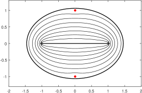
Figure 3: Chebfun implicitly carries out analytic continuation within a Bernstein ellipse bounded approximately by the nearest complex singularity of a function $f$ defined on a real interval. For the function $f(x)=\log(1+x^{2})$ defined on $[-1,1]$, the thick outer curve shows the “Chebfun ellipse” estimate of the region of analyticity plotted by plotregion and the inner curves are contour lines corresponding to errors $|f(x)-p(x)|=10^{-2},10^{-4},\dots,10^{-14}$ (from outside in), where $p$ is the Chebfun approximation, a polynomial of degree $38$. The dots mark the actual branch points of $f$.

Figure 3 illustrates this effect for the function $f(x)=\log(1+x^{2})$, which has branch points at $x=\pm\kern 0.5pti$. By an adaptive process described in chopping , the Chebfun command p = chebfun(’log(1+x^2)’) constructs a polynomial $p$ that matches $f$ on $[-1,1]$ with a maximal error of about $2^{-51}\approx 4.44\times 10^{-16}$; the degree of $p$ for this example is 38.  Typing p(0) to evaluate the polynomial at $x=0$, for example, returns the value $5.5\times 10^{-17}$, accurate to more than 16 digits. What is interesting is that typing p(i/2) also gives an accurate value: $-0.2876820630$, as compared with the true value $\log(0.75)\approx-0.2876820768$. How can we explain this?

In fact, Chebfun is carrying out the Chebyshev analogue of the algorithm of Section 3: it computes a finite sequence of Chebyshev series coefficients, then uses these coefficients to define an approximation $p=\tilde{f}$. Instead of working outward from the unit disk $E$ to larger disks, it is working outward from the unit interval $E$ to so-called Bernstein ellipses, whose algebra is defined by a transplantation of the results of Section 3 by the Joukowski map $(z+z^{-1})/2$. For details, see atap , particularly the discussions of the “Chebfun ellipse” and the command plotregion. According to Theorem 3.1 as transplanted from disks to ellipses, we can expect the number of accurate digits to fall off smoothly, and Figure 3 shows that this is just what is observed.

Analytic continuation in a region bounded by an ellipse is mentioned as Example 3 of franklin , and a detailed analysis of algorithms in this geometry is presented in demtow . Results for ellipses analogous to those of born for disks can be found in wang .

7 Analytic continuation by a chain of disks

The classic idea for analytic continuation, going back to Weierstrass, involves a succession of Taylor expansions, each with its own disk of convergence. In principle, this procedure enables one to track a function along any path where it is analytic, and we recommend the beautifully illustrated discussion in Section 3.6 of Wegert’s Visual Complex Functions wegert . For inexact function data, however, the method is far from promising. There is a small literature on numerical realizations, and a memorable contribution is a 1966 paper by Henrici in which the necessary transformations of series coefficients are formulated in terms of matrix multiplications; see hen66 or (henrici, , sec. 3.6).

To analyze this idea quantitatively, the simplest setting is a channel, essentially the same as the half-strip of Section 4. Specifically, consider the finite-length “stadium” $G$ shown in Figure 4. Given $L>0$, this is the strip of half-width $1$ extending from $x=0$ to $x=L$ together with half-disks of radius 1 at each end. For some $n>0$ and $r\in(0,1),$ we define $h=L/n$ and

$$x_{k}=kh,~{}~{}D_{k}=\{z:\,|z-x_{k}|<1\},~{}~{}D_{k}^{(r)}=\{z:\,|z-x_{k}|<r\}$$ (16)

for $0\leq k\leq n$. We assume $n$ is large enough so that $h<1-r$.

Theorem 7.1

With the definitions of the last paragraph, let $f$ be analytic in $G$ with $\|f\|_{G}\leq 1$ and let $f_{k}$ be analytic in $D_{k}$ with $\|f_{k}\|_{D_{k}}\leq 1$, $0\leq k\leq n-1$. Assume $r\leq 1/2$ and $h\leq 1/4$. Given $\varepsilon\in(0,1)$, define

$$\varepsilon_{k}=\varepsilon^{\kern 0.5pt\exp(-\tilde{e}\kern 0.8ptx_{k})},\quad\tilde{e}={1+2h\over r\log(1/r)}.$$ (17)

If

$$\|f_{0}-f\|_{D_{0}^{(r)}}\leq\varepsilon_{0}$$ (18)

and

$$\|f_{k}-f_{k-1}\|_{D_{k}^{(r)}}\leq\varepsilon_{k},\quad 1\leq k\leq n-1,$$ (19)

then for all sufficiently small choices of $\varepsilon$,

$$\|f_{k-1}-f\|_{D_{k}^{(r)}}\leq\varepsilon_{k},\quad 1\leq k\leq n.$$ (20)

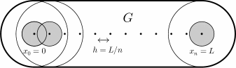
Figure 4: Chain-of-disks analytic continuation of a function $f$ along a channel $G$ of half-width $1$ where it is assumed to be bounded and analytic. One starts with $f$ known to accuracy $\varepsilon_{0}=\varepsilon$ in the shaded disk $D_{0}^{(r)}$ of radius $r$ about $x_{0}=0$; this is then used to construct an expansion to accuracy $\varepsilon_{1}$ in the next shaded disk about $x_{1}=h$, and so on. The best accuracy is achieved with $r=1/e$ and $h\to 0$, with the number of accurate digits diminishing at the rate $\exp(-e\kern 0.3ptx)$.

Proof

We proceed by induction on $k$ in (20). The case $k=1$ follows from (18) by Theorem 3.1 (rescaled by a factor $R=1/r$). Consider step $k+1$, assuming (20) has been established for previous steps. Combining (19) and (20) gives

$$\|f_{k}-f\|_{D_{k}^{(r)}}\leq 2\kern 0.5pt\varepsilon_{k}.$$ (21)

By Theorem 3.1 (with the same rescaling as before), (21) implies

$$\|f_{k}-f\|_{D_{k+1}^{(r)}}\leq(2\kern 0.5pt\varepsilon_{k})^{\alpha},\quad\alpha=1-{\log(1+h/r)\over\log(1/r)}.$$ (22)

(We avoid replacing $\log(1/r)$ by $-\log r$ since it can be confusing to have to remember that $\log r$ is negative.) We are done if we can show

$$(2\kern 0.5pt\varepsilon_{k})^{\alpha}\leq\varepsilon_{k+1}.$$

or by taking logarithms,

$$\left(1-{\log(1+h/r)\over\log(1/r)}\right)(\log 2+\log(\varepsilon_{k}))\leq\log(\varepsilon_{k+1}).$$

By (17), if we divide both sides by the negative quantity $\log(\varepsilon_{k})$, this becomes

$$\left(1-{\log(1+h/r)\over\log(1/r)}\right)\left({\log 2\over\log(\varepsilon_{k})}+1\right)\geq\exp\left({-h-2h^{2}\over r\log(1/r)}\right).$$ (23)

Now suppose for a moment that $\varepsilon_{k}$ is negligible. Then the $\log 2/\log(\varepsilon_{k})$ term goes away and the condition we must verify reduces to

$$1-{\log(1+h/r)\over\log(1/r)}\geq\exp\left({-h-2h^{2}\over r\log(1/r)}\right).$$

A numerical search readily confirms that this holds with a strict inequality over the indicated region $r\in(0,1/2)$, $h\in(0,1/4)$ (the coefficient of the term $-2\kern 0.3pth^{2}$ was introduced to ensure this). Because of the assumption in the theorem statement that $\varepsilon$ is sufficiently small, this establishes (23). ∎

The conclusion of Theorem 20 becomes memorable in the limit $\varepsilon,h\to 0$. The parameter $\tilde{e}$ of (17) is then minimized with the choice $r=1/e$, for which it takes the value $\tilde{e}=e$. We conclude that with this optimal choice of $r$,

The number of accurate digits in chain-of-disks continuation

along a channel of half-width $$1 \exp(-e\kern 0.3ptx)$$ decays at the rate .

In a field as established as complex analysis, it is hard to be sure that anything is entirely new, but I am not aware of a previous estimation of loss of digits at the rate $\exp(-e\kern 0.3ptx)$ for chain-of-disks continuation. The general observation of exponential loss of information is more than a century old. Henrici hen66 writes (his italics)

The early vectors$$\dots$$ must be computed more accurately than the late ones

and he gives credit for related work to Mittag-Leffler, Painlevé, Zeller, and Lewis lewis .

It is interesting to note what our estimates suggest for what might be considered a very natural test problem for analytic continuation. Suppose we have a function like $f(z)=\sqrt{z}$ that is known to be known to be bounded and analytically continuable along any curve in the punctured disk $0<|z|<2$. If we start near $z=1$ with a certain accuracy $\varepsilon$ and go around the origin and back to $z=1$ again, how much accuracy will remain? We will not attempt to give a sharp solution to this problem, but it is the example that motivated our choice of a strip of length $2\pi$ for the numbers quoted in the introduction. Our estimates suggest that the number of accurate digits may be reduced by a factor as great as $(\pi/4)\exp(\pi^{2})\approx\hbox{15,000}$, or $\exp(2\kern 0.4pt\pi e)\approx\hbox{26,000,000}$ for the chain-of-disks method.

8 Conclusion

A compelling presentation of the practical side of analytic continuation can be found in the book to appear by Fornberg and Piret fp . In the case of exactly known functions, although one could use the chain-of-disks idea in principle, Taylor series play little role in practice. A far more powerful approach is to find an analytical method to transform one formula defining a function (a formula being after all a finite object, unlike an infinite set of Taylor coefficients) into another formula with a new region of validity. For the most famous of all examples, the Dirichlet series for the Riemann zeta function converges only for $\hbox{\kern 0.5pt\rm Re}\kern 1.3ptz>1$, but other representations extend $\zeta(z)$ to the whole complex plane.

The present paper has concerned the case of inexactly known functions. Here, for continuation of functions from a disk to a larger disk, or from an interval to an ellipse, algorithms related to Taylor or Chebyshev series are effective, as has been discovered by various authors and we have illustrated by Figure 3 from Chebfun. A third equivalent context would be analytic continuation of a periodic function into a strip by Fourier series. The question is, what can one do to continue a function beyond the disk/ellipse/strip of convergence of its Taylor/Chebyshev/Fourier series? Our theorems show that if all one knows is analyticity and boundedness along certain channels, then accuracy may be lost at a precipitous exponential rate, better than the chain-of-disks but only by a constant. However, the assumption of analyticity just in a channel is more pessimistic than necessary in many applications. Functions arising in applications rarely have natural boundaries or other beautiful pathologies of analytic function theory, however generic such structures may be from a certain abstract point of view; they are far more likely to be analytic everywhere apart from certain poles and branch points. In practice, rational functions are the crucial tool for analytic continuation in such cases, and when they work, their convergence is typically exponential, just as we have found for series-based methods in a disk bgm ; eiermann ; atap . It would be an interesting challenge to develop theorems for meromorphic functions analogous to what we have established here in the analytic case, and a discussion with some of this flavor can be found in millerb .

- (1) Aurentz, J. L., Trefethen, L. N.: Chopping a Chebyshev series. ACM Trans. Math. Softw. 43, 33:1–33:21 (2017)
- (2) Austin, A. P., Kravanja, P., Trefethen, L. N.: Algorithms based on analytic function values in roots of unity. SIAM J. Numer. Anal. 52, 1795–1821 (2014)
- (3) Baker, G. A., Jr., Graves-Morris, P.: Padé Approximants, 2nd ed. Cambridge U. Press (1996)
- (4) Batenkov, D., Demanet, L., Mhaskar, H. N.: Stable soft extrapolation of entire functions. Inverse Problems 35, 015011 (2019)
- (5) Bornemann, F.: Accuracy and stability of computing high-order derivatives of analytic functions by Cauchy integrals. Found. Comput. Math. 11, 1–63 (2011)
- (6) Cannon, J. R., Miller, K.: Some problems in numerical analytic continuation. SIAM J. Numer. Anal. 2, 87–98 (1965)
- (7) Demanet, L., Townsend, A.: Stable extrapolation of analytic functions. Found. Comp. Math. 19, 297–331 (2019)
- (8) Douglas, J.: A numerical method for analytic continuation. Boundary Value Problems in Differential Equations, U. Wisconsin Press, Madison, WI, 179–189 (1960)
- (9) Driscoll, T. A., Hale, N., Trefethen, L. N.: Chebfun Guide. Pafnuty Publications, Oxford (2014). See also www.chebfun.org
- (10) Eiermann, M.: On the convergence of Padé-type approximants to analytic functions. J. Comput. Appl. Math. 10, 219–227 (1984)
- (11) Fornberg, B., Piret, C.: An Illustrated Introduction to Analytic Functions. Book manuscript (2018)
- (12) Franklin, J.: Analytic continuation by the fast Fourier transform. SIAM J. Sci. Stat. Comput. 11, 112–122 (1990)
- (13) Fu, C.-L., Deng, Z.-L., Feng, X.-L., Dou, F.-F.: A modified Tikhonov regularization for stable analytic continuation. SIAM J. Numer. Anal. 47, 2982–3000 (2009)
- (14) Fu, C.-L., Dou, F.-F., Feng, X.-L., Qian, Z.: A simple regularization method for stable analytic continuation. Inverse Problems 24, 1–15 (2008)
- (15) Fu, C.-L., Zhang, Y.-X., Cheng, H., Ma, Y.-J.: Numerical analytic continuation on bounded domains. Engr. Anal. with Boundary Elts. 36, 493–504 (2012)
- (16) Henrici, P.: An algorithm for analytic continuation. SIAM J. Numer. Anal. 3, 67–78 (1966)
- (17) Henrici, P.: Applied and Computational Complex Analysis I: Power Series—Integration—Conformal Mapping—Location of Zeros. John Wiley (1974)
- (18) Hille, E.: Analytic Function Theory II. Chelsea (1987)
- (19) Lewis, G.: Two methods using power series for solving analytic initial value problems. AFC Res. Dev. Rpt. NYO-2881 (1960)
- (20) Miller, K.: Least squares methods for ill-posed problems with a prescribed bound. SIAM J. Math. Anal. 1, 52–74 (1970)
- (21) Miller, K.: Stabilized numerical analytic prolongation with poles. SIAM J. Appl. Math. 18, 346–363 (1970)
- (22) Niethammer, W.: Ein numerisches Verfahren zur analytischen Fortsetzung. Numer. Math. 21, 81–92 (1973)
- (23) Reichel, L.: Numerical methods for analytic continuation and mesh generation. Constr. Approx. 2, 23–39 (1986)
- (24) Rudin, W.: Real and Complex Analysis. McGraw-Hill (1966)
- (25) Stefanescu, I. S.: On the stable analytic continuation with a condition of uniform boundedness. J. Math. Phys. 27, 2657–2686 (1986)
- (26) Trefethen, L. N.: Approximation Theory and Approximation Practice, extended edition. SIAM (2019)
- (27) Vessella, S.: A continuous dependence result in the analytic continuation problem. Forum Math. 11, 695–703 (1999)
- (28) Wang, H., Huybrechs, D.: Fast and accurate computation of Chebyshev coefficients in the complex plane. IMA J. Numer. Anal. 37, 1150–1174 (2016)
- (29) Wegert, E.: Visual Complex Functions. Birkhäuser (2012)