Discrete Laplace Operator Estimation for Dynamic 3D Reconstruction

Abstract

We present a general paradigm for dynamic 3D reconstruction from multiple independent and uncontrolled image sources having arbitrary temporal sampling density and distribution. Our graph-theoretic formulation models the spatio-temporal relationships among our observations in terms of the joint estimation of their 3D geometry and its discrete Laplace operator. Towards this end, we define a tri-convex optimization framework that leverages the geometric properties and dependencies found among a Euclidean shape-space and the discrete Laplace operator describing its local and global topology. We present a reconstructability analysis, experiments on motion capture data and multi-view image datasets, as well as explore applications to geometry-based event segmentation and data association.

1 Introduction

Image-based dynamic reconstruction addresses the modeling and estimation of the spatio-temporal relationships among non-stationary scene elements and the sensors observing them. This work tackles estimating the geometry (i.e. the Euclidean coordinates) of a temporally evolving set of 3D points using as input unsynchronized 2D feature observations with known imaging geometry. Our problem, which straddles both trajectory triangulation and image sequencing, naturally arises in the context of uncoordinated distributed capture of an event (e.g. crowd-sourced images or video) and highlights a pair of open research questions: How to characterize and model spatio-temporal relationships among the observations in a data-dependent manner? What role (if any) may available spatial and temporal priors play within the estimation process? The answer to both these questions is tightly coupled to the level of abstraction used to define temporal associations and the scope of the assumptions conferred upon our observations. More specifically, the temporal abstraction level may be quantitative or ordinal (i.e. capture time-stamps vs. sequencing), while the scope of the assumptions may be domain-specific (i.e. temporal sampling periodicity/frequency, choice of shape/trajectory basis) or cross-domain (physics-based priors on motion estimates).

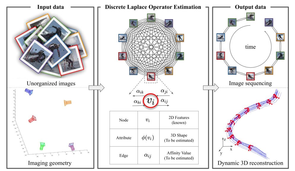
Figure 1: Multi-view capture produces a set of unorganized 2D observations. Our graph formulation of dynamic reconstruction jointly estimates sequencing and 3D geometry. Imagery adapted from [27].

Estimating either absolute or relative temporal values for our observations would require explicit assumptions on the observed scene dynamics and/or the availability of sampling temporal information (e.g. image time-stamps or sampling frequency priors). In the absence of such information or priors, we strive to estimate observation sequencing based on data-dependent adjacency relations defined by a pairwise affinity measure. Towards this end, we make the following assumptions: A1) 2D observations are samples of the continuous motion of a 3D point set; A2) the (unknown and arbitrary) temporal sampling density allows approximate local linear interpolation of 3D geometry; and A3) temporal proximity implies spatial proximity, but not vice-versa (e.g. repetitive or self-intersecting motion). Under such tenets, we can address multi-view capture scenarios comprised of unsynchronized image streams or the more general case of uncoordinated asynchronous photography.

We solve a dictionary learning instance enforcing a discrete differential geometry model, where each dictionary atom corresponds to a 3D estimate, while the set of sparse coefficients describes the spatio-temporal relations among our observations. Our contributions are:

• A graph-theoretic formulation of the dynamic reconstruction problem, where 2D observations are mapped to nodes, 3D geometry are node attributes, and spatio-temporal affinities correspond to graph edges.

• The definition and enforcement of spatio-temporal priors, (e.g. anisotropic smoothness, topological compactness/sparsity, and multi-view reconstructability) in terms of the discrete Laplace operator.

• Integration of available per-stream (e.g. intra-video) sequencing info into global ordering priors enforced in terms of the Laplacian spectral signature.

2 Related work

Dynamic reconstruction in the absence of temporal information is an under-constrained problem akin to single view reconstruction [5, 6, 18, 29, 28, 24]. Some prior work in trajectory triangulation operate under the assumptions of known sequencing info and/or constrained motion priors. Along these lines, Avidan and Shashua [6] estimate dynamic geometry from 2D observations of points constrained to linear and conical motions. However, under the assumption of dense temporal motion sampling, the concept of motion smoothness has been successfully exploited [25, 26, 45, 46, 35, 42, 43, 36, 30, 31]. Park et al. [25] triangulate 3D point trajectories by the linear combination of Direct Cosine Transform trajectory bases with the constraint of a reprojection system. Such a trajectory basis method has low reconstructability when the number of the bases is insufficient and/or the motion correlation between object and camera is large. In [26], Park et al. select number of bases by an N-fold cross validation scheme. Zhu et al. [45] apply $L_{1}$-norm regularization to the basis coefficients to force the sparsity of bases and improve the reconstructability by including a small number of keyframes, which requires user interaction. Valmadre et al. [35] reduce the number of trajectory bases by setting a gain threshold depending on the basis null-space and propose a method using a high-pass filter to mitigate low reconstructability for scenarios having no missing 2D observations. Zheng et al. [43, 42] propose a dictionary learning method to estimate the 3D shape with partial sequencing info, assuming 3D geometry estimates may be approximated by local barycentric interpolation (i.e. self-expressive motion prior) and developed a bi-convex framework for jointly estimating 3D geometry and barycentric weights. However, uniform penalization of self-expressive residual error and fostering symmetric weight coefficients, handicap the approach against non-uniform density sampling. Vo et al. [36] present a spatio-temporal bundle adjustment which jointly optimizes camera parameters, 3D static points, 3D dynamic trajectories and temporal alignment between cameras using explicit physics priors, but require frame-accurate initial time offset and low 2D noise. Efforts at developing more detailed spatio-temporal models within the context of NRSFM include [2, 3, 4].

Temporal alignment is a necessary pre-processing step for most dynamic 3D reconstruction methods. Current video synchronization or image sequencing [8, 21, 39, 23, 14, 9] rely on the image 2D features, foregoing the recovery of the 3D structure. Feature-based sequencing methods like [8, 39, 33] make different assumptions on the underlying imaging geometry. For example, while [8] favors an approximately static imaging geometry, [39] prefers viewing configurations with large baselines. Basha et al. [21] overcomes the limitation of static cameras and improves accuracy by leveraging the temporal info of frames in individual cameras. Padua et al. [23] determines spatio-temporal alignment among a partially order set of observation by framing the problem as mapping of $N$ observations into a single line in $\mathbb{R}^{N}$, which explicitly imposes a total ordering. Unlike previous methods, Gaspar et al [16] propose a synchronization algorithm without tracking corresponding feature between video sequences. Instead, they synchronize two videos by the relative motion between two rigid objects. Tuytelaars et al. [34] determined sequencing based on the approximate 3D intersections of viewing rays under an affine reference frame. Ji et al. [19] jointly synchronize a pair of video sequences and reconstruct their commonly observed dense 3D structure by maximizing the spatio-temporal consistency of two-view pixel correspondences across video sequences.

3 Graph-based Dynamic Reconstruction

For a set of 2D observations in a single image with known viewing parameters, there is an infinite set of plausible 3D geometry estimates which are compliant with a pinhole camera model. We posit that for the asynchronous multi-view dynamic reconstruction of smooth 3D motions, the constraints on each 3D estimate can be expressed in terms of its temporal neighborhood. That is, we aim to enforce spatial coherence among successive 3D observations without the reliance on instance-specific spatial or temporal models. It is at this point that we come to a chicken-egg problem, as we need to define a notion of temporal neighborhood in the context of uncontrolled asynchronous capture w/o timestamps or sampling frequency priors. To address this conundrum we use spatial proximity as a proxy for temporal proximity, which (as prescribed by our third assumption, i.e. A3) is not universally true. Moreover, given that observed events ”happen” over a continuous 1D timeline, we would also like to generalize our notion proximity into one of adjacency, so as to be able to explicitly define the notion of a local neighborhood. Towards this end, we pose the dynamic 3D reconstruction problem in terms of discrete differential geometry concepts.

3.1 Notation and Preliminaries

We consider $P$ dynamic 3D points $\{\mathbf{X}_{p}\}$ observed in $N$ images $\{\mathcal{I}_{n}\}$ with known intrinsic and extrinsic camera matrices $\mathbf{K}_{n}$ and $\mathbf{M}_{n}$. The 2D observation of $\mathbf{X}_{p}$ in $\mathcal{I}_{n}$ is denoted by $\mathbf{x}_{n,p}$, while its 3D position is denoted by $\mathbf{X}_{n,p}$.

Euclidean Structure Matrix. The position of all 3D points across all images is denoted by the matrix

$$\mathbb{X}=\begin{bmatrix}\mathbf{X}_{11}&\dots&\mathbf{X}_{1P}\\ \vdots&\ddots&\vdots\\ \mathbf{X}_{N1}&\dots&\mathbf{X}_{NP}\end{bmatrix}$$ (1)

where each row vector $\mathbf{X}_{np}\in\mathbb{R}^{3}$ specifies the 3D Euclidean coordinates of a point. Each matrix row $\mathbb{X}_{n,:}\in\mathbb{R}^{3\times P}$, represents the 3D shape of the $P$ points in frame $n$.

Structure Motion Graph. We define a fully connected graph $G=(V,E)$, and map each input image $\mathcal{I}_{n}$ to a vertex $v_{n}\in V$. A multi-value function $\phi(\cdot)$ maps a vertex into a point in the shape space, allowing the interpretation $\mathbb{X}=\left[\phi(v_{1});\dots;\phi(v_{N})\right]$. Edge weight values $e_{ij}\in E$ are defined by an affinity function $\alpha(\cdot)$ relating points in our shape space, such that $e_{ij}=\alpha_{ij}=\alpha\left(\phi(v_{i}),\phi(v_{j})\right)$.

Discrete Laplace operator. The Laplace operator $\Delta$ is a second differential operator in $n-$dimensional Euclidean space, which in Cartesian coordinates equals to the sum of unmixed second partial derivatives. For a weighted undirected graph $G=(V,E)$, the discrete Laplace operator is defined in terms of the Laplacian matrix:

$$\mathbb{L}=\mathbb{L}_{[\mathbb{A}]}=\mathbb{D}-\mathbb{A}=diag(\mathbb{A}\cdot\mathbf{1})-\mathbb{A}$$ (2)

where $\mathbb{A}$ is the graph’s symmetric affinity matrix, whose values $\mathbb{A}_{ij}$ correspond to the edge weights $e_{ij}\in\mathbb{R}_{\geq 0}$, and $\mathbb{D}$ is the graph’s diagonal degree matrix, whose values are the sum of the corresponding row in $\mathbb{A}$. $\mathbb{L}$ is positive semi-definite, yielding $\mathbf{x}^{\top}\mathbb{L}\mathbf{x}\geq 0,\;\forall\mathbf{x}\in\mathbb{R}^{n}$. When convenient, we obviate the explicit dependence of $\mathbb{L}$ on $\mathbb{A}$.

Affinity Matrix Decomposition. The pairwise affinity function $\alpha(\cdot)$ (relating our 3D estimates) is implicitly defined in terms of the estimated entries $\mathbb{A}_{ij}$. Importantly, these affinity values also encode the graph’s local topology (i.e. connectivity). Given the a priori unknown topology and distribution of our 3D estimates, we make the following design choices: 1) $\mathbb{A}$ is not assumed to be symmetric, yielding a directed structure graph. 2) we explicitly model the decomposition $\mathbb{A}=\mathbb{D}\mathbb{W}$, which follows from Eq. (2),

$$\mathbb{L}=\mathbb{D}-\mathbb{A}=\mathbb{D}(\mathbb{I}-\mathbb{W})$$ (3)

This decomposition decouples the estimation of each node’s degree value (encoded in $\mathbb{D}$), from the relative affinity weight values for the node’s local neighborhood (encoded in $\mathbb{W}$).

3.2 Geometric Rationale

We leverage the interdependencies among our 3D motion estimates $\mathbb{X}$ and its discrete Laplace operator $\mathbb{L}$, through an optimization framework for their joint estimation. In practice, $\mathbb{L}$ describes the topology of the given structure $\mathbb{X}$ in terms of an affinity function $\alpha(\cdot)$. The values $\alpha_{ij}$ constitute the entries of the affinity matrix $\mathbb{A}_{ij}$ relating the 3D shapes observed at frames $i$ and $j$. These individual values are determined through the estimation of the $\mathbb{D}$ and $\mathbb{W}$ variables within our optimization framework. Hence, the affinity $\alpha$ function will not be explicitly defined, but rather its values will be instantiated from the results of our optimization, which builds upon the following geometric observations.

Remark 1 (Anisotropic Smoothness Prior).

The norm of the Laplacian’s linear form ($\mathbb{LX}$), tends to vanish when any given function value $\phi(v_{i})$ approximates the (affinity-weighted) average of $\phi(v_{j\neq i})$ in its local neighborhood. This follows from the point-wise Laplacian definition

$$\left[\mathbb{LX}\right]_{i,:}=(\Delta\phi)(v_{i})=\sum\nolimits_{j}^{N}\mathbb{A}_{ij}\left[\phi(v_{i})-\phi(v_{j})\right]$$ (4)

This implies approximately linear 3D motion segments allow accurate barycentric interpolation from as little as two neighboring 3D motion samples. Conversely, the penalty for poorly approximated non-linear motion segments may be mitigated by the multiplicative contribution of the degree value towards the affinity value, i.e. $\mathbb{A}_{ij}=\mathbb{D}_{ii}\mathbb{W}_{ij}$

Remark 2 (Collapsing Neighborhood Prior).

The trace of the Laplacian’s quadratic form ($\mathbb{X^{\top}LX}$) tends to vanish as the local neighborhood becomes sparser and more compact, this follows from

$$tr(\mathbb{X}^{\top}\mathbb{L}\mathbb{X})=\sum\nolimits_{i,j}^{N}\mathbb{A}_{ij}||\phi(v_{i})-\phi(v_{j})||_{2}^{2}$$ (5)

This implies sparsity in global affinity, while non-zero $\mathbb{A}_{ij}$ values imply proximity among 3D samples $\mathbb{X}_{i,:}$ and $\mathbb{X}_{j,:}$.

Remark 3 (Spectral Sequencing Prior).

Any line mapping of $V$ into a vector $\mathbf{f}\in\mathbb{R}^{N}$ constitutes an ordering of the graph vertices. Accordingly, when $\mathbf{f}$ is a known and constant affinity preserving mapping, the non-trivial minimization of $\mathbf{f}^{\top}\mathbb{L}\mathbf{f}$ will yield entries in $\mathbb{L}$ approximating the affinities encoded in $\mathbf{f}$. This follows from

$$\mathbf{f}^{\top}\mathbb{L}\mathbf{f}=\sum\nolimits_{i,j}^{N}\mathbb{A}_{ij}\left(f_{i}-f_{j}\right)^{2}$$ (6)

This implies enforcing global sequencing priors by coupling $\mathbb{L}$’s spectral signature to an input vector $\mathbf{f}$.

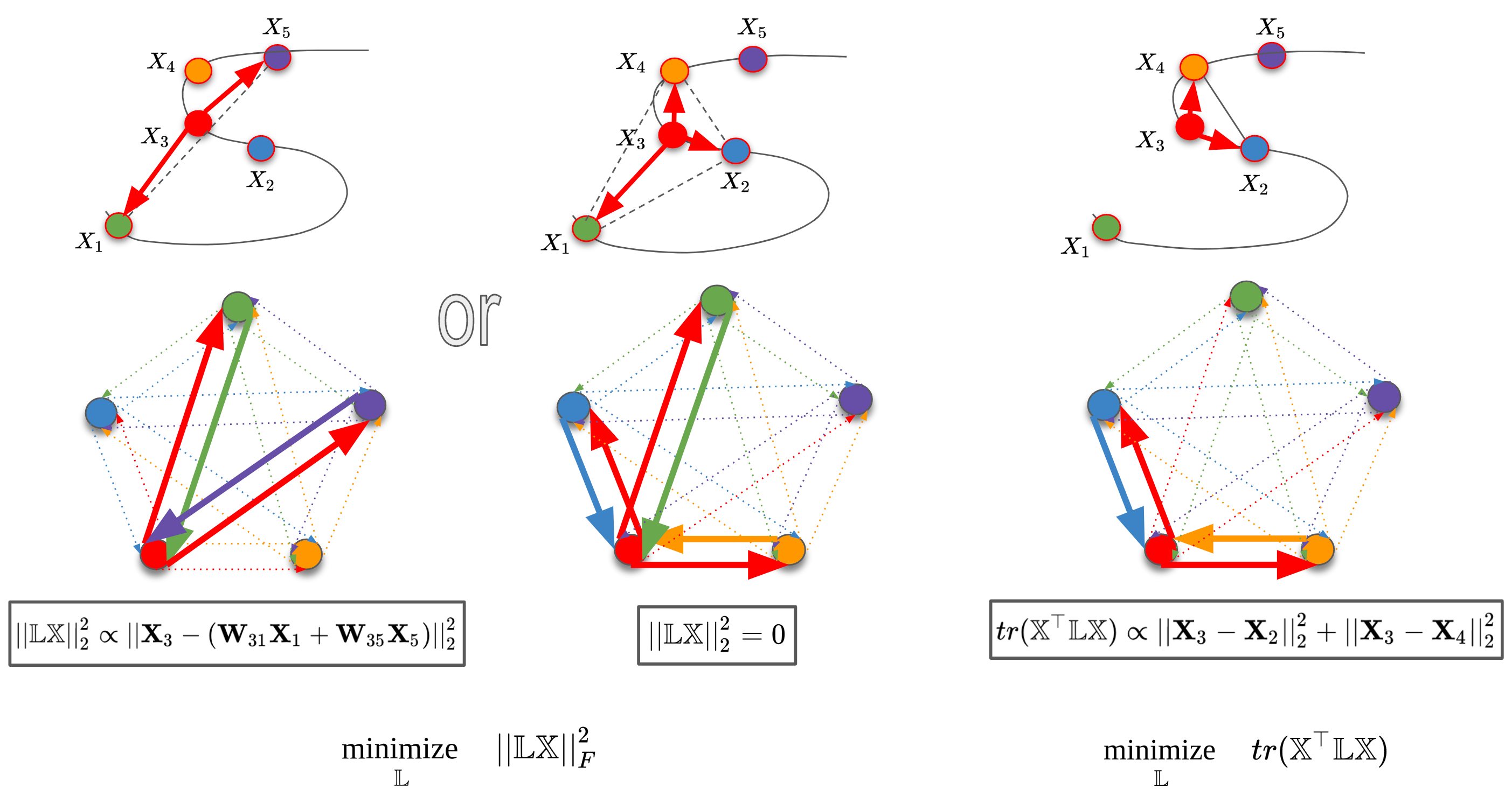
Figure 2: Geometry of Remarks 1 & 2. At top: Arrows denote selected neighboring samples and dashed lines their convex hull. At bottom: Corresponding graph edge structure.

3.3 Optimization Cost Function

Based on the geometric properties encoded by the discrete Laplace operator the formulate the optimization problem:

$$\underset{\mathbb{X},\mathbb{L}}{\text{min}}\quad\mathcal{S}\left(\mathbb{L}\mathbb{X}\right)+\mathcal{T}\left(\mathbb{X}^{\top}\mathbb{L}\mathbb{X}\right)+\mathcal{R}\left(\mathbb{L},\Theta\right)+\mathcal{O}\left(\mathbb{X},\Theta\right),$$ (7)

where $\Theta=\{\{\mathbf{x}_{np}\},\{\mathbf{K}_{n}\},\{\mathbf{M}_{n}\}\}$ denotes the aggregation of all input 2D observations and their camera parameters. Each cost function term addresses a particular aspect of our optimization. $\mathcal{S}(\cdot)$ fosters local smoothness, $\mathcal{T}(\cdot)$ fosters a linear topological structure, $\mathcal{R}(\cdot)$ fosters strong convergence among viewing rays, while $\mathcal{O}(\cdot)$ reduces reprojection errors. For simplicity, we define the problem variables in terms of $\mathbb{L}$ and $\mathbb{X}$. However, given the explicit dependence of $\mathbb{L}$ on $\mathbb{A}$, we’ll redefine the joint optimization of Eq. (7), as a tri-convex optimization problem over $\mathbb{X}$, $\mathbb{D}$, and $\mathbb{W}$.

The next two sections describe the functional models ($\mathcal{S}$, $\mathcal{T}$, $\mathcal{R}$, and $\mathcal{O}$) utilized in Eq. (7), the structure of the estimation variables ($\mathbb{X}$, $\mathbb{D}$, and $\mathbb{W}$), and the constraints applicable to them. We present two variants of our general framework, addressing, respectively, the absence and the estimation of global temporal sequencing priors on the elements of $\{\mathcal{I}_{n}\}$.

4 Solving for Asynchronous Photography

We consider an unordered image set $\{\mathcal{I}_{n}\}$, and rely on the Collapsing Neighborhood Prior to estimate an affinity function matrix whose connectivity approximates a chain-structure connectivity. We interpret such connectivity as temporal ordering relations among our observations.

Enforcing anisotropic smoothness. The functional form

$$\mathcal{S}\left(\mathbb{L}\mathbb{X}\right)=\frac{1}{P}||\mathbb{D}(\mathbb{I}-\mathbb{W})\mathbb{X}||_{F}^{2}$$ (8)

defines the first term of Eq. (7). Minimizing $\mathcal{S}$ w.r.t. $\mathbb{X}$ attracts function values $\phi(v_{i})$ towards the convex hull defined by all $\phi(v_{j\neq i})$ in its local neighborhood. Conversely, minimizing $\mathcal{S}$ w.r.t. $\mathbb{L}$ (i.e. $\mathbb{D}$, $\mathbb{W}$) fosters the selection of neighboring nodes whose mappings $\phi(v_{j\neq i})$ facilitate barycentric interpolation. Here, selection refers to assigning non-zero values $\mathbb{A}_{ij}$ in the affinity matrix.

The values in each row of $\mathbb{W}$ (i.e. $\mathbb{W}_{i,:}$) represent the relative affinity weights for $v_{i}$. Hence, we enforce 1) the sum of each row equal to 1, and 2) strict non-negativity of all entries in $\mathbb{W}$.Moreover, $\mathbb{D}$ represents the out-degree for each node in the directed graph, akin to a global density estimate. We decouple node degree values from the relative affinity weights in $\mathbb{W}$. We enforce strictly positive degree values $\mathbb{D}_{ii}\geq\epsilon$, requiring connectivity to at least one adjacent node.

Enforcing Neighborhood Locality. For a directed graph, we define the trace of the Laplacian quadratic form as

$$tr(\mathbb{X}^{\top}\overset{\text{\tiny$\leftrightarrow$}}{\mathbb{L}}\mathbb{X})=\sum\nolimits_{i,j}^{N}\mathbb{A}_{ij}||\mathbb{X}_{i,:}-\mathbb{X}_{j,:}||_{2}^{2}\\$$ (9)

Where $\overset{\text{\tiny$\leftrightarrow$}}{\mathbb{L}}=\mathbb{L}_{[\mathbb{A}+\mathbb{A}^{\top}]}$ combines the outdegree and indegree Laplacian matrix, and is compliant with the definition in Eq. (5). Diagonal entries of the $N\times N$ matrix $\mathbb{X}^{\top}\mathbb{L}_{[\mathbb{A}+\mathbb{A}^{\top}]}\mathbb{X}$ are the Laplacian quadratic form for each dimension of $\phi()$, and the functional form of $\mathcal{T}$ in Eq. (7) is given by their sum:

$$\begin{split}\mathcal{T}\left(\mathbb{X}^{\top}\mathbb{L}\mathbb{X}\right)=\frac{\lambda_{1}}{P}\sum\nolimits_{i,j}^{N}\mathbb{D}_{ii}\mathbb{W}_{ij}||\mathbb{X}_{i,:}-\mathbb{X}_{j,:}||_{2}^{2}\end{split}$$ (10)

Minimizing $\mathcal{T}$ w.r.t. $\mathbb{X}$ (i.e. fixing $\mathbb{A}$) attracts the estimates $\phi(v_{j\neq i})$ of neighboring elements to be near to $\phi(v_{i})$. Conversely, minimizing $\mathcal{T}$ w.r.t. $\mathbb{A}$, fosters the selection of nearby nodes to form a compact neighborhood, as defined by the weighted sum of the magnitude of the difference vectors $\phi(v_{i})-\phi(v_{j\neq i})$, $\forall\mathbb{A}_{ij}\neq 0$.

Enforcing Observation Ray Constrains. We penalize the distance of a 3D point $\mathbb{X}_{np}$ to its known viewing ray using $\mathbf{d}_{np}=||(\mathbf{X}_{np}-\mathbf{C}_{n})\times\mathbf{r}_{np}||_{2},$ where $\mathbf{r}_{np}$ is a unit vector parallel to the viewing ray $\mathbf{R}_{n}^{\top}\mathbf{K}_{n}^{-1}[\mathbf{x}_{np}^{\top}\quad 1]^{\top}$ and camera pose parameters are given by $\mathbf{M}_{n}=[\mathbf{R}_{n}|-\mathbf{R}_{n}\mathbf{C}_{n}]$ [43]. The functional form of $\mathcal{O}$ from Eq. (7) is

$$\mathcal{O}\left(\mathbb{X},\Theta\right)=\sum\nolimits_{n,p}^{N,P}\frac{\lambda_{2}}{NP}||\mathbf{d}_{np}||_{2}^{2},$$ (11)

which is quadratic for $\mathbb{X}$. The value of $\lambda_{2}$ depends on the 2D noise level and the mean camera-to-scene distance.
Enforcing Multi-view Reconstructability. Viewing geometry plays a determinant role in the overall accuracy of our 3D estimates (see section 7 for a detailed analysis). Intuitively, for moderate-to-high 2D noise levels, the selection of temporally adjacent cameras with small baselines will amplify 3D estimation error. In order to foster the selection of cameras having favorable convergence angles among viewing rays corresponding to the same feature track, we define the functional form of $\mathbb{R}$ from Eq. (7) as

$$\mathcal{R}\left(\mathbb{L},\Theta\right)=\frac{\lambda_{3}}{NP}\sum\nolimits_{i,j,p}^{N,N,P}\left(\mathbb{D}_{ii}\mathbb{W}_{ij}\left(\mathbf{r}_{ip}\cdot\mathbf{r}_{jp}\right)\right)^{2}$$ (12)

5 Solving for Unsynchronized Image Streams

Given an image set comprised of the aggregation of multiple image streams, we ascertain partial sequencing (i.e. within disjoint image subsets). We use this info in two different ways: First, we enforce spatial smoothness among successive observations from a common stream. Second, we integrate disjoint local sequences into a global sequencing estimate we enforce through our optimization.
Enforcing Intra-Sequence Coherence. We define $\mathbb{W}=\mathbb{W}_{var}+\mathbb{W}_{prior}$, where $\mathbb{W}_{var}$ constitutes the variable component of our estimation, while $\mathbb{W}_{prior}$ encodes small additive values for the immediately prior and next frames from the same image stream. The collapsing neighborhood prior will enforce such pseudo-adjacent 3D estimates to be similar.
Manipulating the Spectral Signature of $\mathbb{L}$. For a given global sequencing prior, in the form of a line embedding $\mathbf{f}\in\mathbb{R}^{N}$ of all our graph nodes, we modify Eq. (10) to be

$$\begin{split}\mathcal{T}\left(\mathbf{f}^{\top}\mathbb{L}\mathbf{f}\right)=\frac{\lambda_{1}}{P}\sum\nolimits_{i,j}^{N}\mathbb{D}_{ii}\mathbb{W}_{ij}\left(\mathbf{f}_{i}-\mathbf{f}_{j}\right)^{2}.\end{split}$$ (13)

We now describe how we determine such line embedding $\mathbf{f}$.
Integrating Global Sequencing Priors. Our goal is to integrate preliminary (e.g. initialization) geometry estimates, $\mathbb{X}^{init}$, with reliable but partial sequencing information (e.g. single video frame sequencing) into a global sequencing prior. Towards this end, we pose image sequencing from a given 3D structure $\mathbb{X}$ as a dimensionality reduction instance, where the goal is to find a line mapping which preserves (as much as possible) pairwise proximity relations among 3D estimates. While using Euclidean distance as a pairwise proximity measure is suitable for approximately linear motion, non-linear motion manifolds (i.e. repetitive or self-intersecting motions) may collapse temporally distant observations to proximal locations in the line embedding.
Arc Distance through Dynamic Time Warping. We define approximate 3D trajectory arc distance for shapes within sequenced images streams, as the sum of 3D line segment lengths among adjacent observations, see Fig. 3(a). To generalize this notion across image streams, we perform global approximate inter-sequence registration through Dynamic Time Warping (DTW). Our goal is to assign to each 3D estimate $t^{a}_{i}$ along trajectory $a$ the closest line segment $(t^{b}_{j},t^{b}_{j+1})$ in each of the other trajectories $b\neq a$, without violating any sequencing constraints in our assignments, which we define

$$t^{a}_{i}\rightarrow(t^{b}_{j},t^{b}_{j+1})\quad\nexists\quad t^{a}_{k>i}\rightarrow(t^{b}_{l<j},t^{b}_{l+1})\;\;\forall a\neq b$$ (14)

Once all assignments are made, inter-sequence arc-length between $t^{a}_{i}$ and $t^{b}_{l}$ is trivially computed as the sum of 1) distance to the element $t^{b}_{*}$ in the line segment $(t^{b}_{j},t^{b}_{j+1})$ closest to the $t^{b}_{l}$, plus 2) the intra-sequence arc distance between $t^{b}_{*}$ and $t^{b}_{l}$. Fig. 3(b) illustrates the arc distance from points between $t^{a}_{i}$ and $t^{b}_{l}$ as the length of green line.

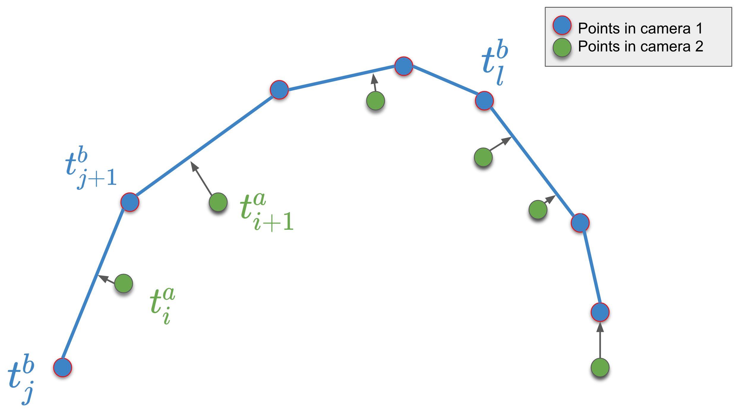
(a) Matching with DTW.

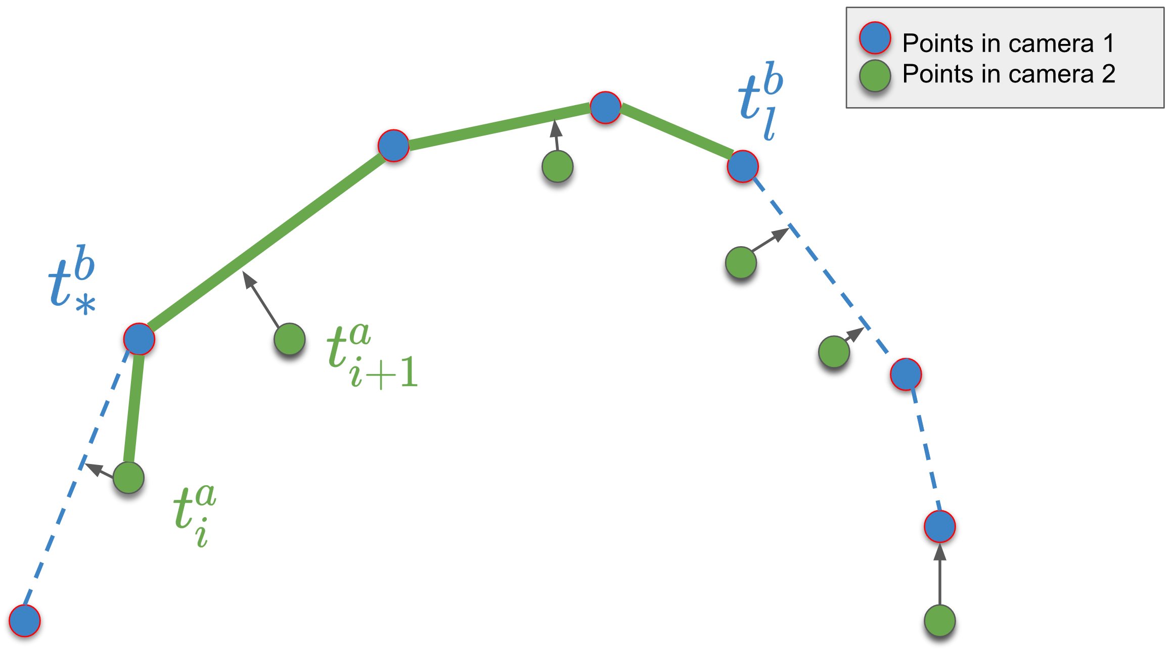
(b) Arc distance

Figure 3: Arc distance between two observations of the same 3D point across different image streams.

Dimensionality Reduction Methods. We use arc length to define a pair-wise distance matrix ${\mathbb{Z}}$, from which we attain a vector embedding $\mathbf{f}\in\mathbb{R}^{n}$ through Spectral Ranking (SR) [15, 13] and Multidimensional Scaling (MDS) [1]. Sequencing is attained by sorting $\mathbf{f}$. Alternatively, we interpret ${\mathbb{Z}}$ as a complete graph’s weight matrix and find the approximate shortest Hamiltonian path (SHP). Table 1 compares these methods operating on ${\mathbb{Z}}$ and the Euclidean distance matrix ${\mathbb{Z}^{E}}$, both matrices were computed from $\mathbb{X}^{init}$ and $\mathbb{X}^{opt}$, which denote respectively, the initial 3D structure and the estimated 3D structure after our optimization.

		Linear motion		Nonlinear motion		Repeating motion
		$\mathbb{X}^{init}$	$\mathbb{X}^{opt}$	$\mathbb{X}^{init}$	$\mathbb{X}^{opt}$	$\mathbb{X}^{init}$	$\mathbb{X}^{opt}$
SR	$\mathbb{Z}^{E}$	0.9956	0.9996	0.9807	0.9991	0.6754	0.7140
	$\mathbb{Z}$	0.9965	1	0.9570	1	0.9711	0.9934
MDS	$\mathbb{Z}^{E}$	0.9943	1	0.7614	0.7044	0.6421	0.6553
	$\mathbb{Z}$	0.9961	1	0.8741	1	0.9316	0.9732
SHP	$\mathbb{Z}^{E}$	1	1	0.4368	0.9996	0.3329	0.7912
	$\mathbb{Z}$	1	1	0.5325	0.9996	0.3947	0.7934

Table 1: Kendall rank correlation vs. ground truth ordering for sequencing attained from initial and estimated structure.

6 Optimization

Eq. (7) is a tri-convex function for variable blocks $\mathbb{X}$, $\mathbb{W}$ and $\mathbb{D}$. We use the ACS [17] strategy, alternatively optimizing over each variable block while fixing the other two. For the first iteration, we initialize $\mathbb{D}$ and $\mathbb{X}$ (to be described), then we alternatively optimize over each variable blocks in the order of $\mathbb{W}$, $\mathbb{D}$ and $\mathbb{X}$ until (thresholded) convergence of our cost function among successive iterations.

Optimizing over $\mathbb{X}$. While variable blocks $\mathbb{W}$ and $\mathbb{D}$ are fixed, the cost function (7) is a quadratic equation for block $\mathbb{X}$ without any constraints. The solution for this quadratic programming problem is the set of variable values found at the zeros of the derivative of the cost function.

Optimizing over $\mathbb{W}$. With $\mathbb{X}$ and $\mathbb{D}$ fixed, minimizing $\mathcal{S}\left(\mathbb{L}\mathbb{X}\right)$, $\mathcal{T}\left(\mathbb{X}^{\top}\mathbb{L}\mathbb{X}\right)$, $\mathcal{O}\left(\mathbb{X},\Theta\right)$ and $\mathcal{R}\left(\mathbb{L},\Theta\right)$, respectively, yield a quadratic equation, linear equation and constant value for $\mathbb{W}$, making the cost function a quadratic equation for $\mathbb{W}$

$$\underset{\mathbb{W}}{\text{min}} \frac{1}{P}||\mathbb{D}(\mathbb{I}-\mathbb{W})\mathbb{X}||_{F}^{2}+\frac{\lambda_{1}}{P}\sum\limits_{ij}^{N}\mathbb{D}_{ii}\mathbb{W}_{ij}||\mathbb{X}_{i,:}-\mathbb{X}_{j,:}||_{2}^{2}$$ (15)

$$+\frac{\lambda_{3}}{NP}\sum\nolimits_{i,j,p}^{N,N,P}\left(\mathbb{D}_{ii}\mathbb{W}_{ij}\left(\mathbf{r}_{ip}\cdot\mathbf{r}_{jp}\right)\right)^{2}$$

s.t. $$\mathbb{W}\mathbf{1}_{N\times 1}=\mathbf{1}_{N\times 1},\quad\mathbb{W}\geq 0$$

Each row of $\mathbb{W}$ is independent and is solved as a quadratic programming problem with linear constrains. We optimize each row in parallel by the Active-Set method in [11].

Optimizing over $\mathbb{D}$. When $\mathbb{X}$ and $\mathbb{W}$ are fixed, optimizing Eq. (7) yields a quadratic equation in terms of the diagonal values of $\mathbb{D}$. We optimize the same equation as Eq. (15), but with linear constrains $\{tr(\mathbb{D})=1,\mathbb{D}\geq 0\}$, normalizing the outdegree sum to one.

Optimizing for the spectral sequencing prior When optimizing over $\mathbb{W}$ or $\mathbb{D}$, the matrix $\mathbb{X}$ is replaced by a vector $\mathbf{f}$, computed from the current estimate of $\mathbb{X}$, through one of the dimensionality reduction methods described earlier (e.g. MDS applied to $\mathbb{Z}$) Hence, the second term becomes

$$\mathbf{f}^{\top}\overset{\text{\tiny$\leftrightarrow$}}{\mathbb{L}}\mathbf{f}=\sum\nolimits_{ij}^{N}\mathbb{D}_{ii}\mathbb{W}_{ij}(\mathbf{f}_{i}-\mathbf{f}_{j})^{2}\\$$ (16)

When using MDS as the dimensionality reduction method, $\mathbf{f}$ approximately preserves the pairwise Arc distance, allowing direct implementation within Eq. (16). When using SR, $\mathbf{f}$ corresponds to the graph’s Fiedler vector, whose entry values range from -1 to 1; requiring a uniform scaling in order to match the range of the current structure estimate $\mathbb{X}$.

Initialization. We initialize the degree matrix to be $\mathbb{D}_{ii}=1/N$. We initialize the 3D structure $\mathbb{X}^{init}_{n,:}$ observed in $\mathcal{I}_{n}$ by the approximate two-view pseudo-triangulation of each viewing ray $\mathbf{r}_{np}$ with its corresponding viewing ray $\mathbf{r^{*}}_{m\neq n,p}$ from the most convergent image $\mathcal{I}_{m}$, which is the $\mathcal{I}_{m}$ with the minimum aggregated pseudo-triangulation error when considering all commonly observed points.

7 Structure Reconstruction Accuracy.

              

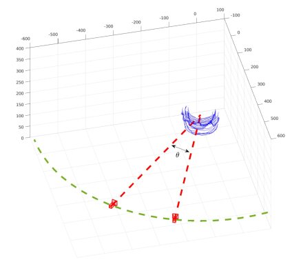
(a) Convergence angle $\theta$

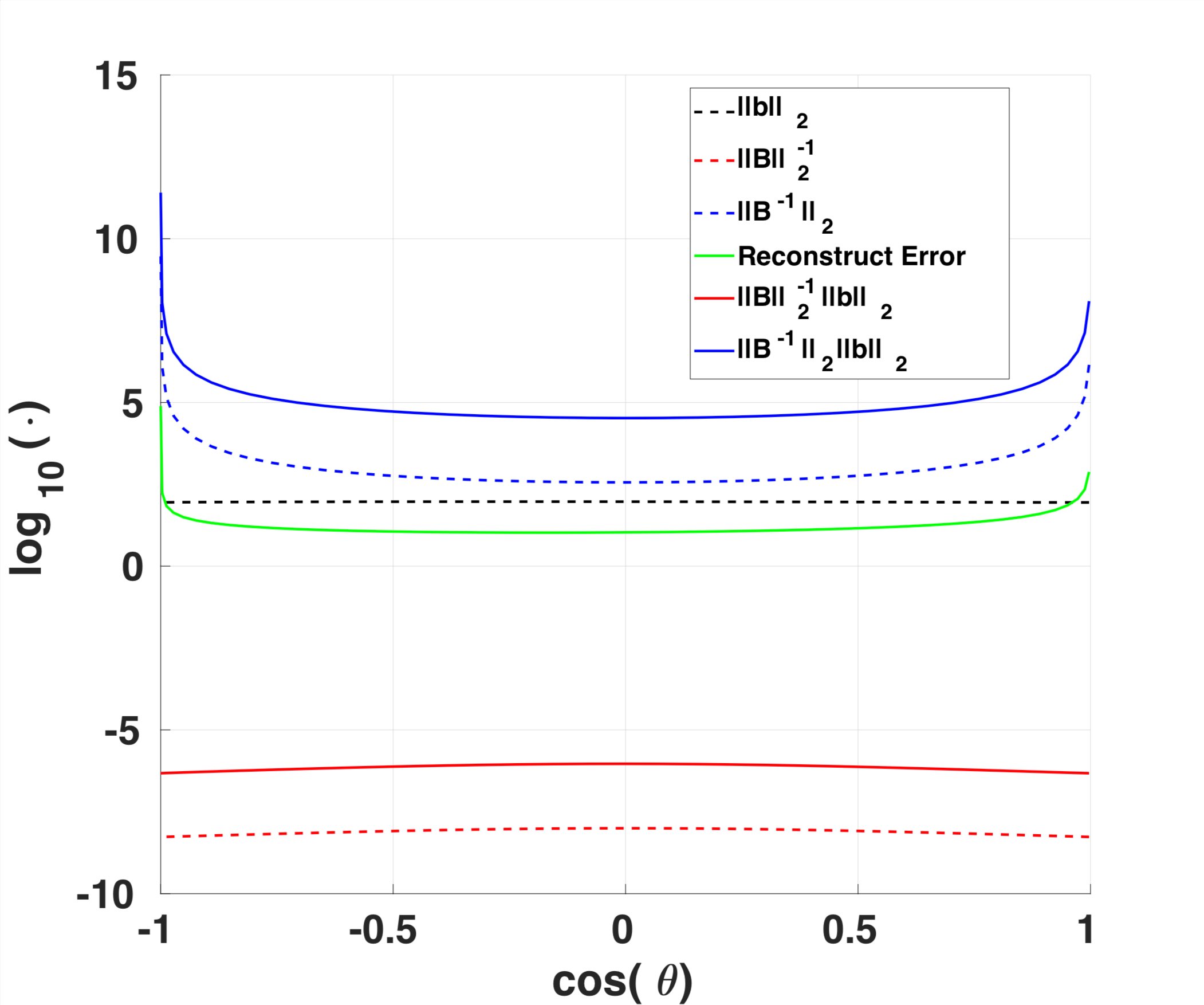
(b) $\mathbb{B}$ term analysis

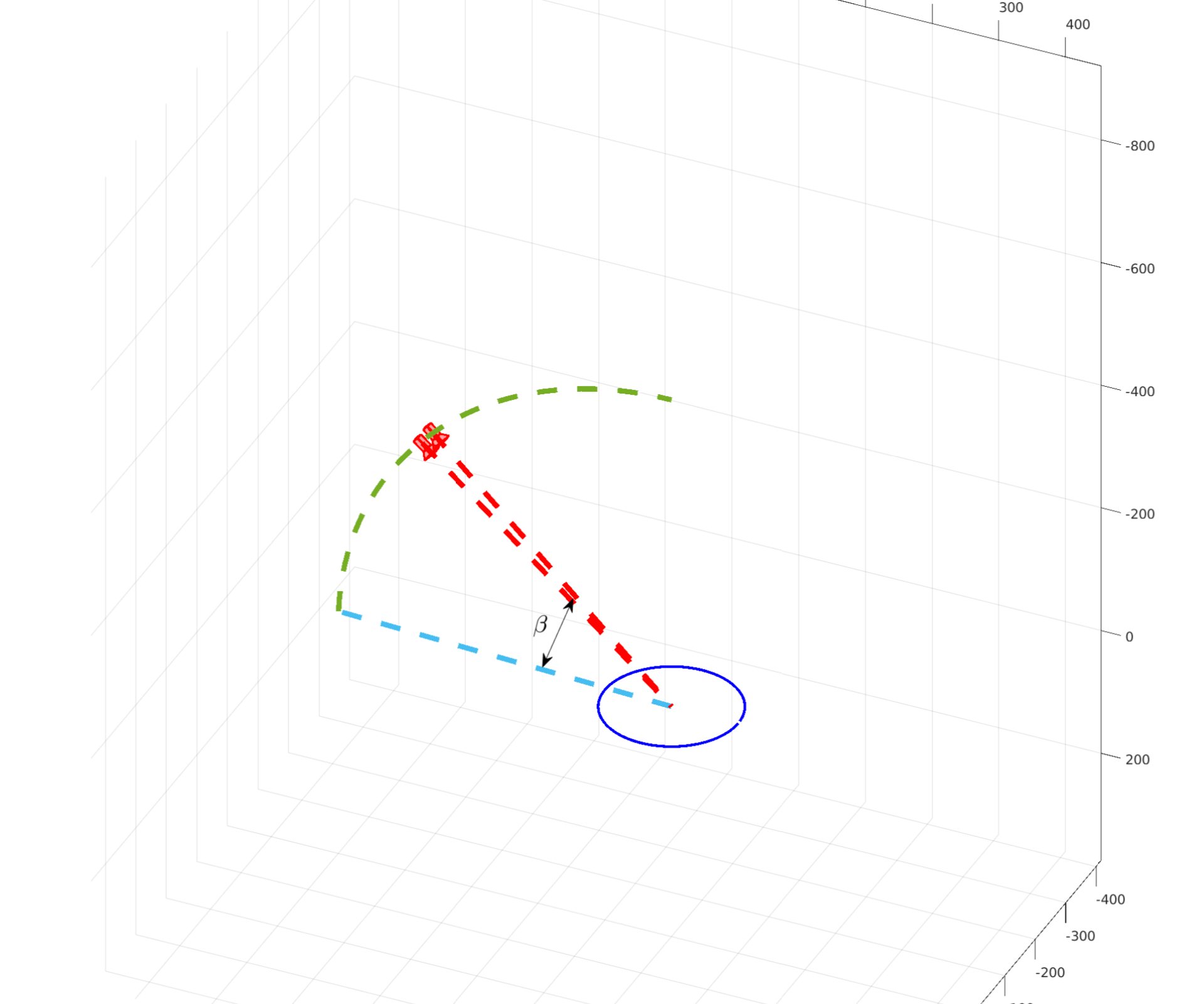
(c) Incidence angle $\beta$

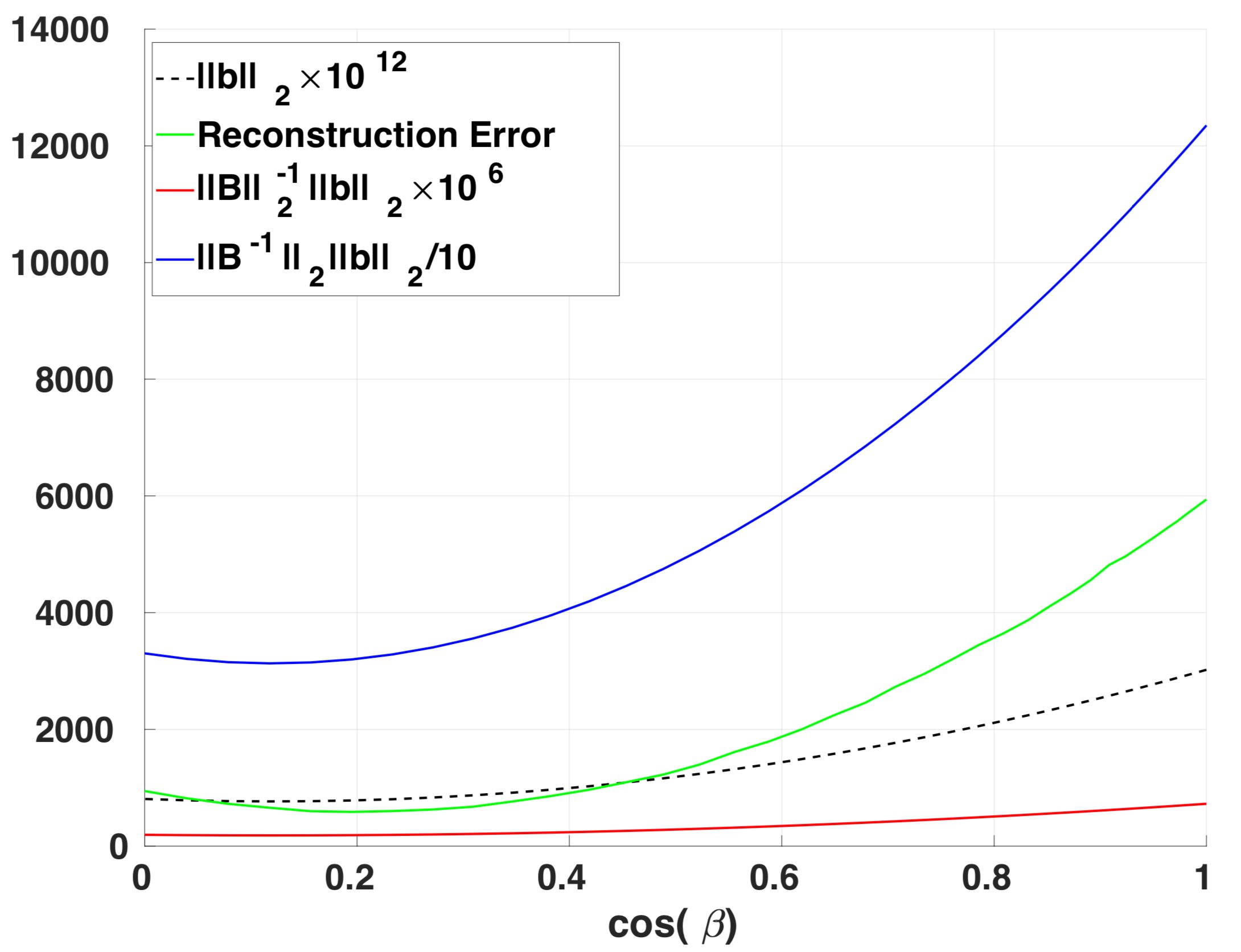
(d) $\mathbf{b}$ term analysis

Figure 4: In (a,b) error bounds specified in Eq. (21) get ”tighter” and reconstruction error is reduced when neighboring viewing rays near orthogonality. In (c,d) as the angle $\beta$ is close to $\pi/2$, both reconstruction error and $\mathbf{||b||}_{2}$ decrease.

We analyze how the Lapalacian linear and quadratic forms influence the accuracy of our estimates of $\mathbb{X}$, assuming: 1) $\mathbb{L}$ is fixed, 2) encodes ground truth temporal adjacency, and 3) noise free 2D observations. This equates to optimizing Eq. (7) while omitting terms $\mathcal{O}$ and $\mathcal{R}$, yielding

$$\underset{\mathbb{X}}{\text{min}}\quad\frac{1}{P}||\mathbb{L}\mathbb{X}||_{F}^{2}+\frac{\lambda_{1}}{P}tr(\mathbb{X}^{\top}\overset{\text{\tiny$\leftrightarrow$}}{\mathbb{L}}\mathbb{X})$$ (17)

We denote the ground truth structure as $\mathbb{X}^{*}$ and since each point is independently estimated, we analyze the condition of one point per shape. Then, $\mathbb{X}$ as a point along a viewing ray is $\mathbb{X}_{n,:}=\mathbb{X}^{*}_{n,:}+l_{n}\mathbf{r}_{n},$ where the unknown variables $l_{n}$ are the signed distance from ground truth along the viewing ray, and $|\mathbf{l}|$ is the reconstruction error (i.e. depth error). Eq. (17) is an unconstrained quadratic programming problem, solved by setting the derivative over $l$ to zero; yielding to

$$\mathbb{B}\mathbf{l} =\mathbf{b}$$ (18)

$$\mathbb{B} =(\mathbb{L}^{\top}\mathbb{L}+\lambda_{1}\overset{\text{\tiny$\leftrightarrow$}}{\mathbb{L}})\odot\begin{bmatrix}\mathbf{r}_{1}^{\top}\mathbf{r}_{1}&\dots&\mathbf{r}_{N}^{\top}\mathbf{r}_{1}\\ \vdots&\ddots&\vdots\\ \mathbf{r}_{1}^{\top}\mathbf{r}_{N}&\dots&\mathbf{r}_{N}^{\top}\mathbf{r}_{N}\end{bmatrix}$$ (19)

$$\mathbf{b}_{n} =(\mathbb{L}^{\top}_{:,n}\mathbb{L}\mathbb{X}^{*}+\lambda_{1}\overset{\text{\tiny$\leftrightarrow$}}{\mathbb{L}}_{n,:}\mathbb{X}^{*})\mathbf{r}_{n}$$ (20)

where $\mathbb{B}$ is an $N\times N$ matrix and $\mathbf{b}$ is an $N\times 1$ vector whose $n$-th element is $\mathbf{b}_{n}$, and $\mathbb{L}_{:,n}$ denotes the $n$-th column of $\mathbb{L}$ and $\overset{\text{\tiny$\leftrightarrow$}}{\mathbb{L}}_{n,:}$ denotes the $n$-th row. From Eq. (18), we attain the lower and upper bounds for reconstruction error as

$$||\mathbb{B}||_{2}^{-1}||\mathbf{b}||_{2}\leq||\mathbf{l}||_{2}\leq||\mathbb{B}^{-1}||_{2}||\mathbf{b}||_{2}$$ (21)

Imaging geometry convergence. We consider two cameras alternating the capture of a motion sequence, which are placed sufficiently far from the motion center $\mathbf{c}$, such that the viewing ray convergence angle for all joints can be approximated by the angle $\theta$ between the cameras to the motion center. We vary $\theta$ from 0 to $\pi$ as in Fig. 4(a).and evaluate the reconstruction error and upper bounds, which as shown in Fig. 4(b) decrease as viewing rays approach orthogonality.

3D motion observability. The vector $\overset{\text{\tiny$\leftrightarrow$}}{\mathbb{L}}_{n,:}\mathbb{X}^{*}$ in Eq. (20), lies on a local motion plane formed by $\mathbb{X}^{*}_{n,:}$ and it’s two neighboring points. Similarly,each row in $\mathbb{L}\mathbb{X}^{*}$ will also be a vector on a local motion plane. For smooth motion under dense sampling, a triplet of successive local motion planes can be approximated by a common 3D plane $\pi_{n}$. Hence, the vector $\mathbb{L}^{\top}_{:,n}\mathbb{L}\mathbb{X}^{*}+\lambda_{1}\overset{\text{\tiny$\leftrightarrow$}}{\mathbb{L}}_{n,:}\mathbb{X}^{*}$ will be contained in $\pi_{n}$, yielding smaller values of $\mathbf{b}_{n}$ as $\pi_{n}$ and the viewing rays $\mathbf{r}_{n}$ near orthogonality.In Fig. 4(c), we consider a circle motion observed by two cameras with constant convergence angle, pointing to the motion center. In this configuration, $||\mathbb{B}||_{2}^{-1}$ and $||\mathbb{B}^{-1}||_{2}$ are nearly constant. We vary the angle $\beta$ between the viewing directions and the motion plane $\pi_{n}$. Fig. 4(d) shows more accurate reconstruction is attained for viewing directions near orthogonal to the motion plane.

8 Experiments

Figure 5: Reconstruction error for motion capture data under different conditions. Reported averages over 20 executions.

   

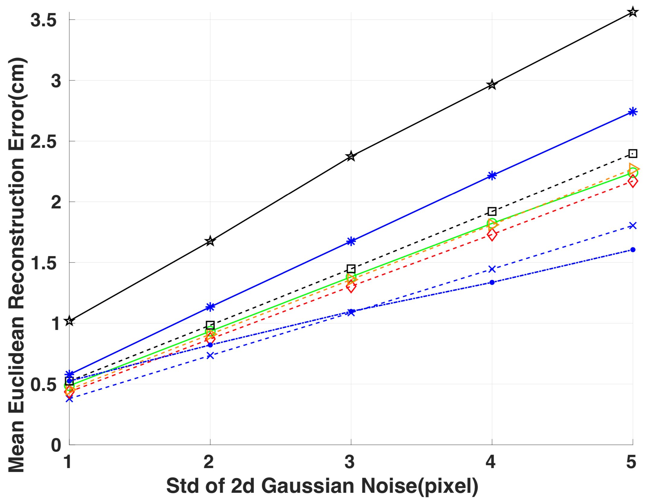
(a) Noise level

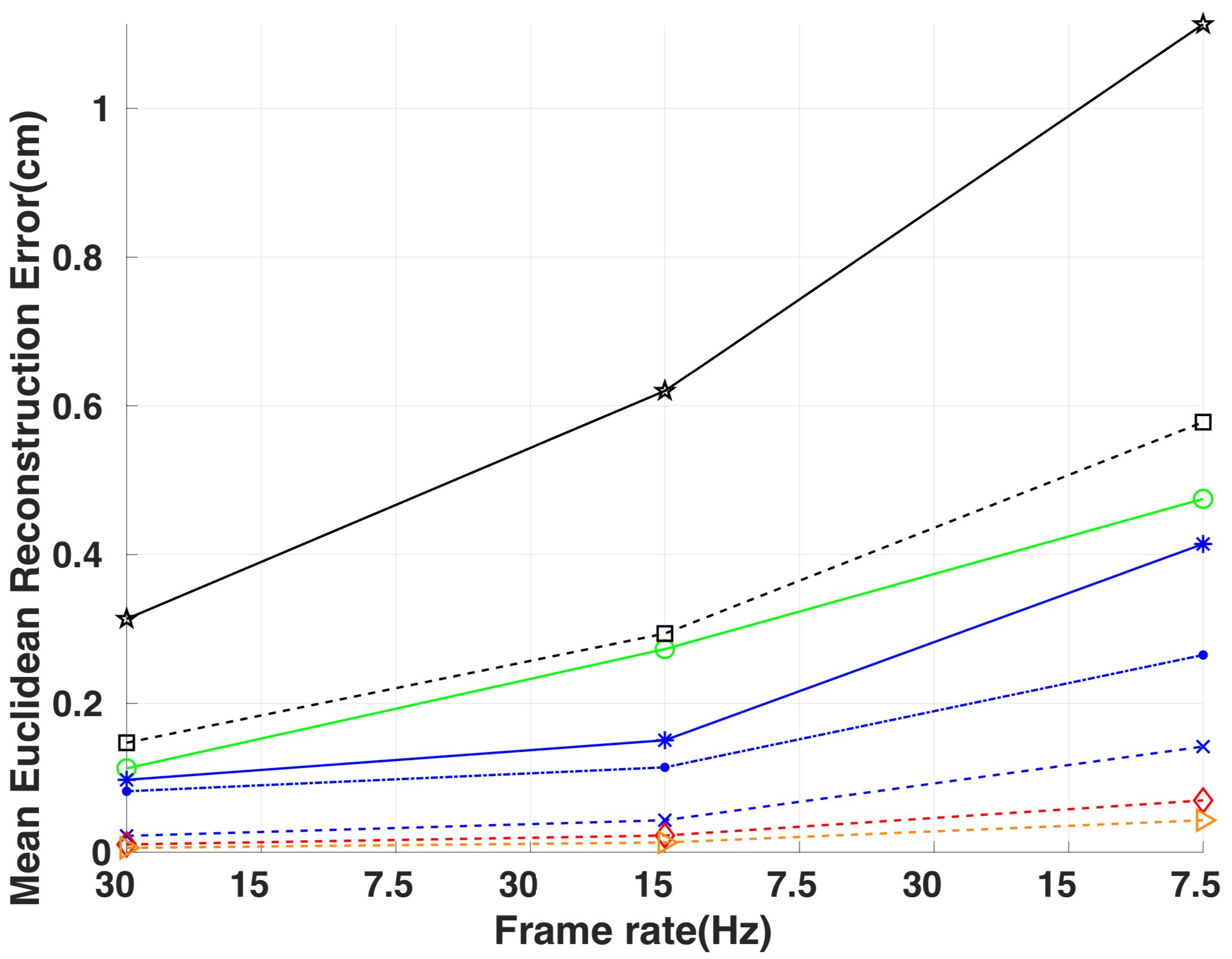
(b) Frame rates

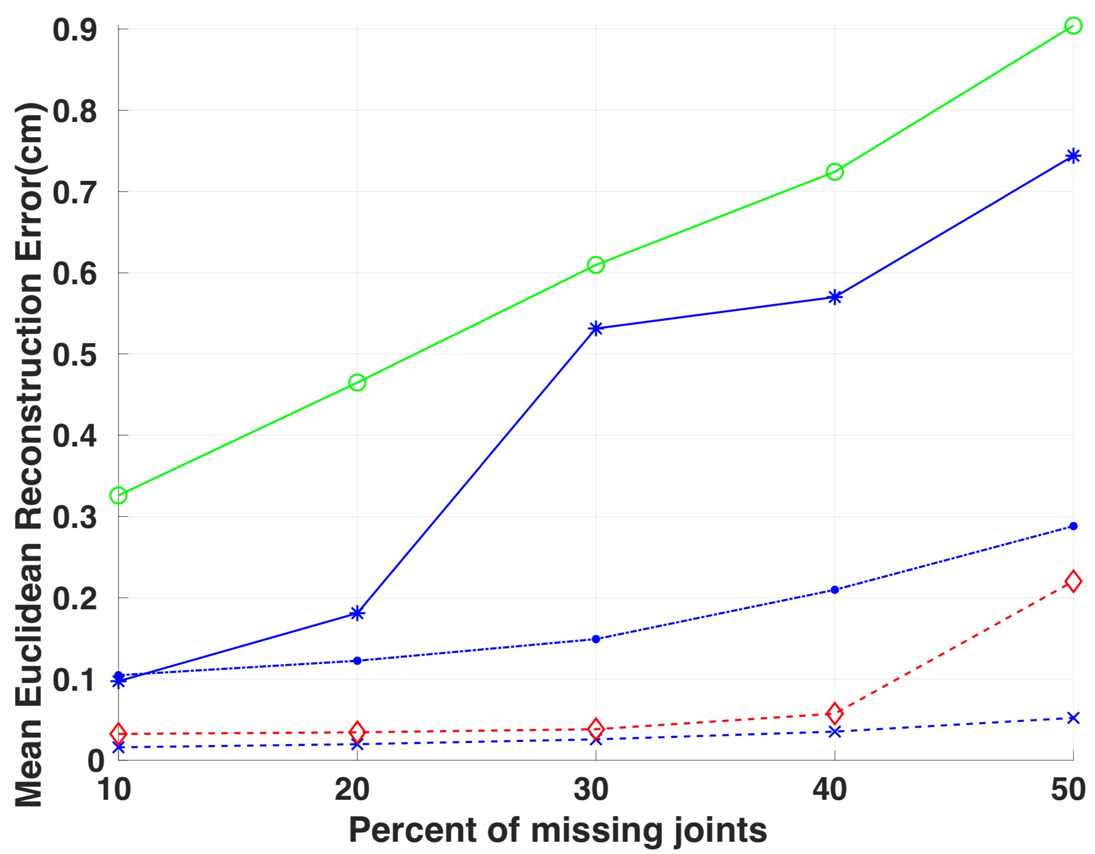
(c) Missing points

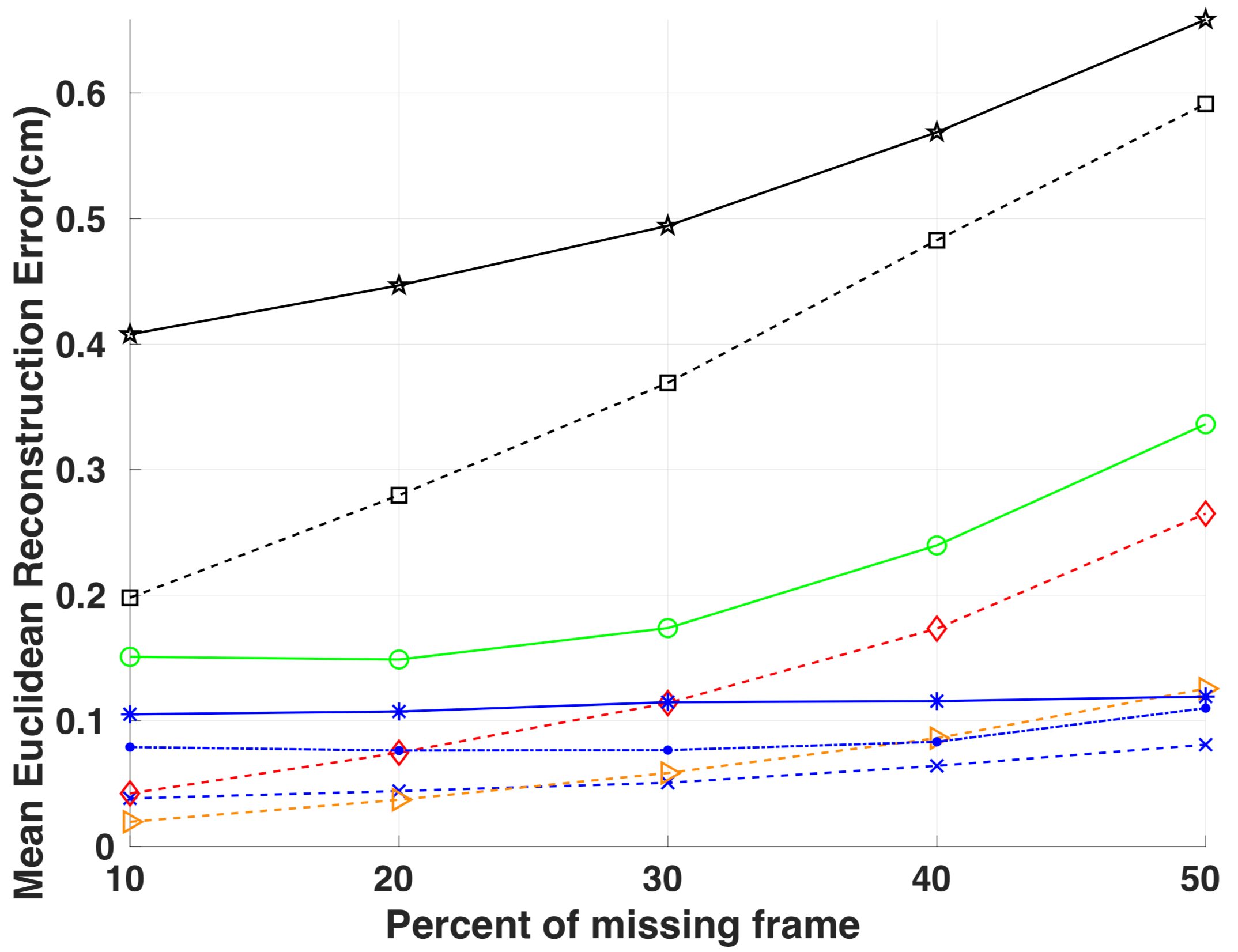
(d) Nonuniform density

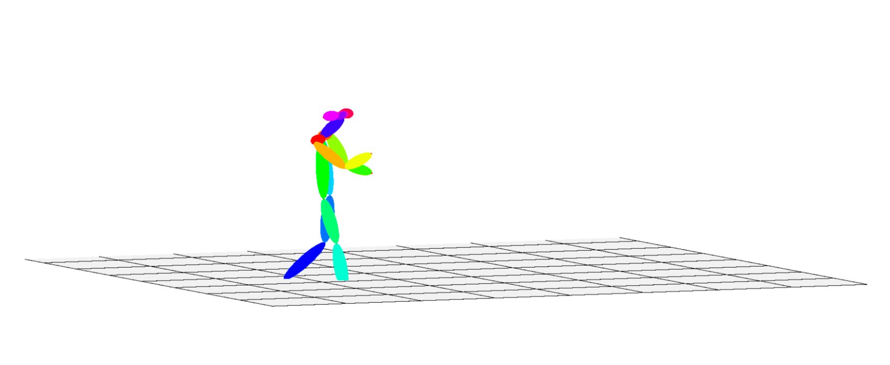
(a) Juggler.

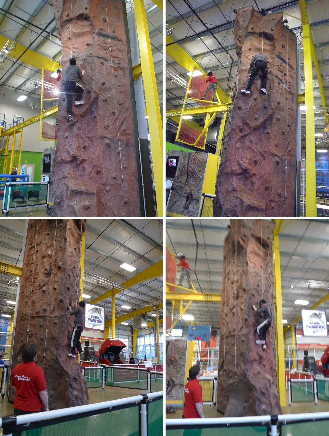
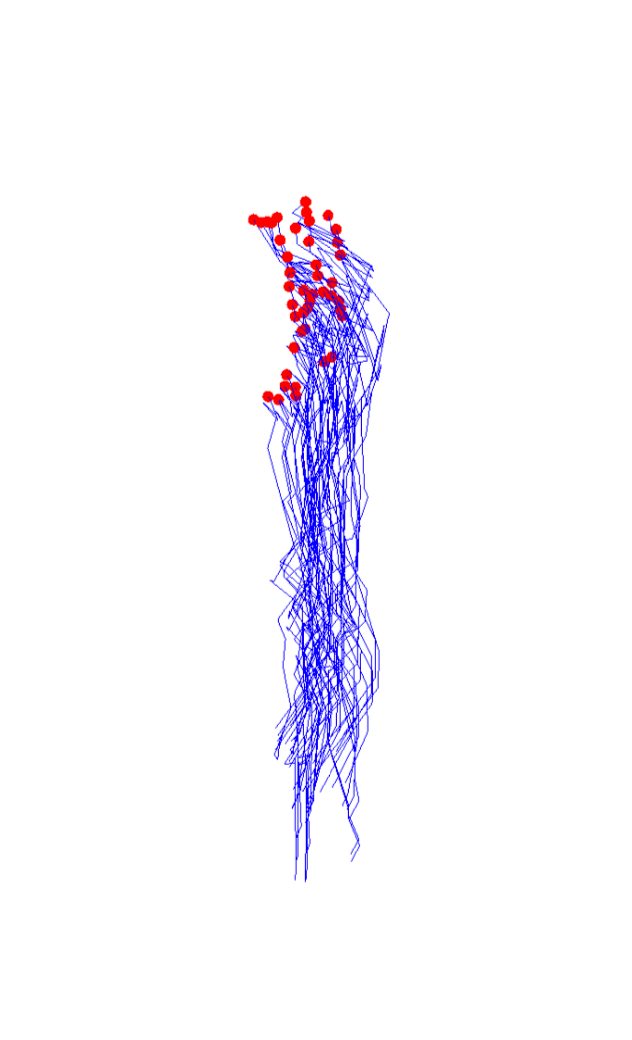
(b) Climb

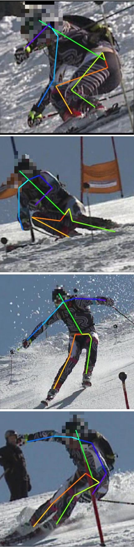
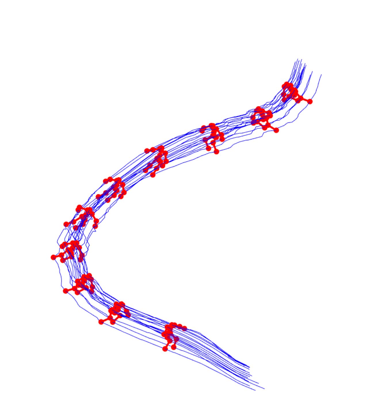
(c) Ski

	data type	motion type	solver type	number of cameras	number of frames	number of joints	frame rate	kendall rank correlation
Juggler	unsynchronized videos	repeating motion	DLOE+MDS+$\mathbb{W}_{prior}$	4	80	18	6.25	0.8816
Climb	unsynchronized images	linear motion	DLOE+MDS+$\mathbb{W}_{prior}$	5	27	45	N/A	0.8689
Ski	unsynchronized videos	nonlinear motion	DLOE+MDS+$\mathbb{W}_{prior}$	6	137	17	N/A	0.9526

Figure 6: Experiments on multi-view image capture. All datasets were devoid of concurrent observations.

  

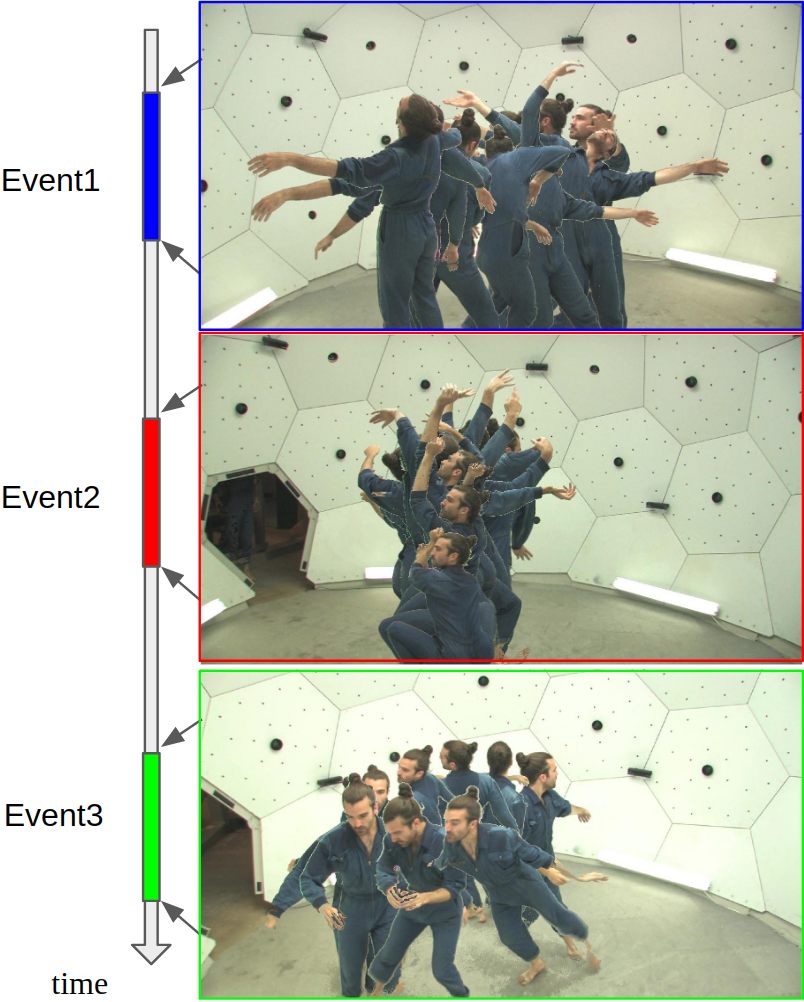
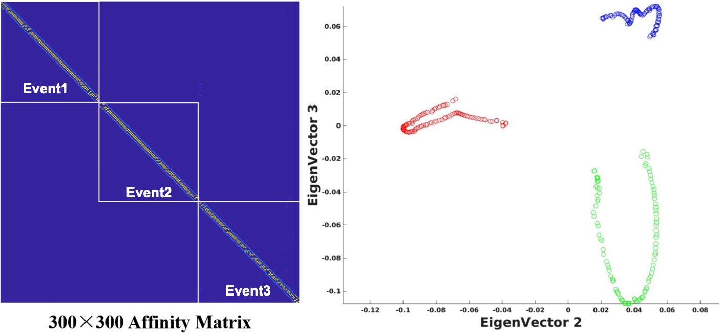
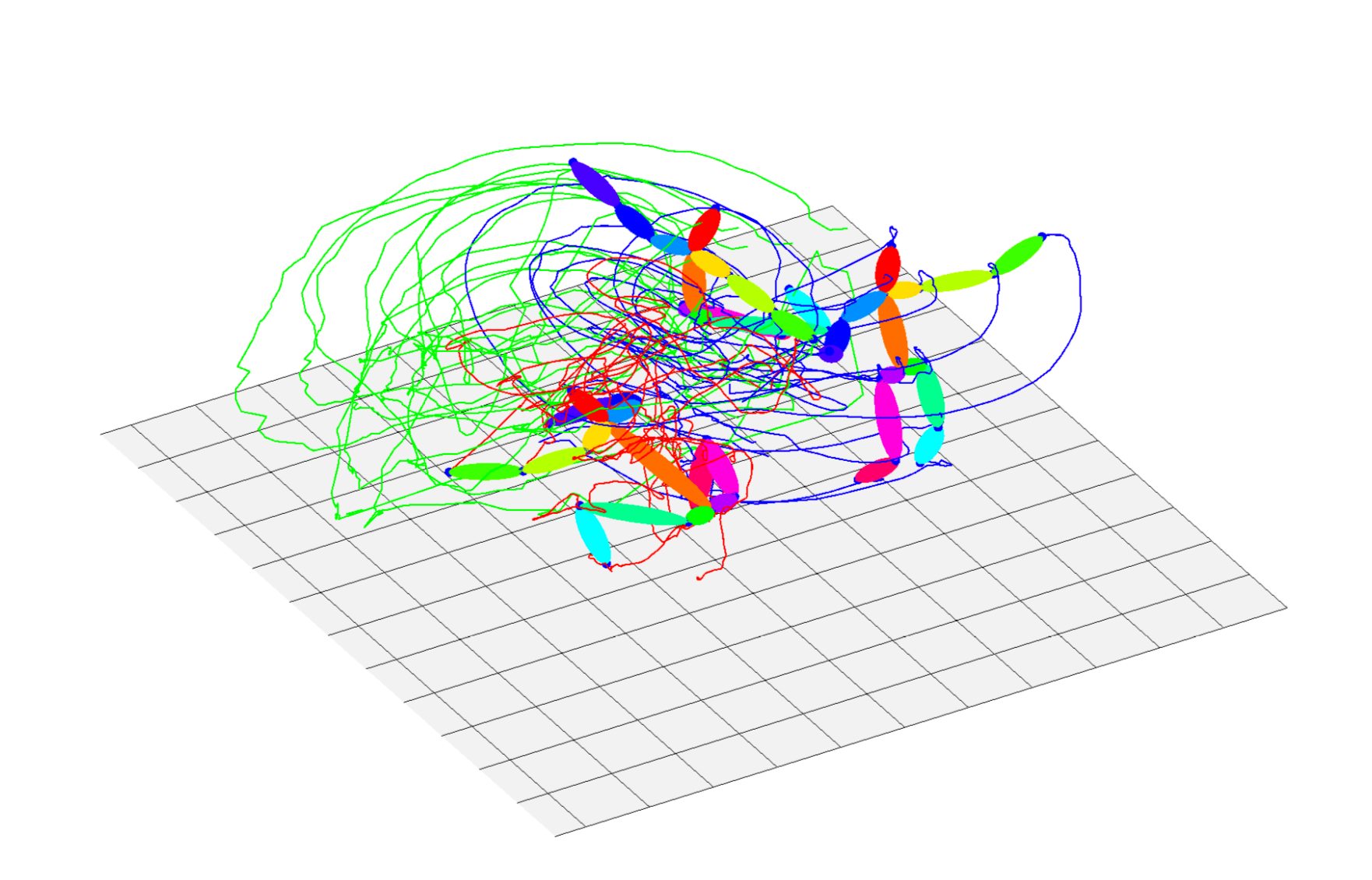
(a) Event segmentation

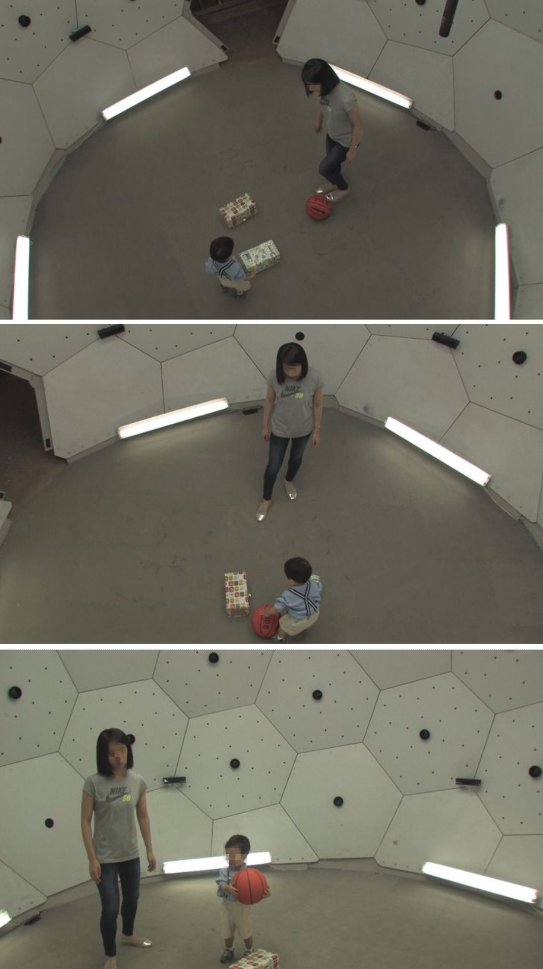
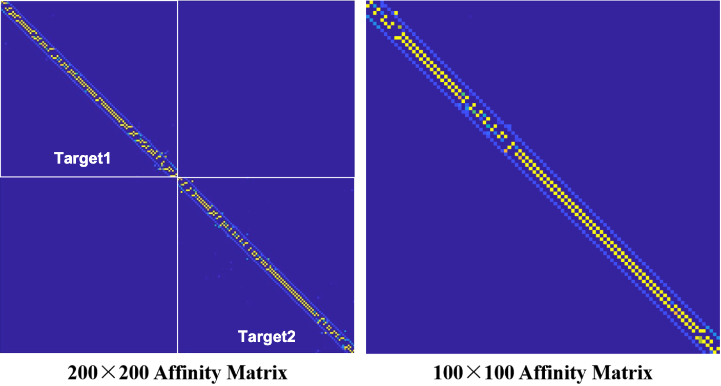
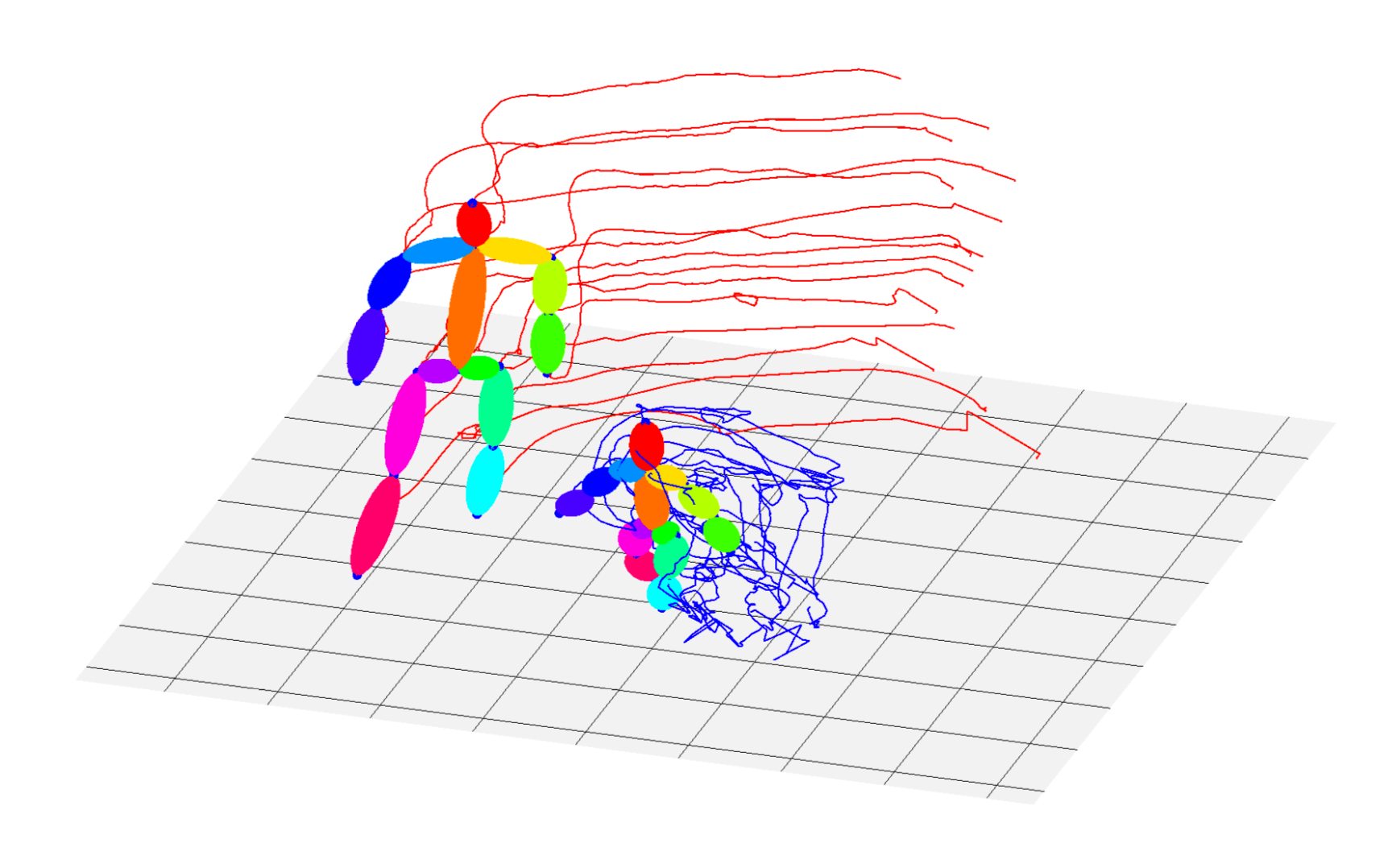
(b) Multi-Target scenario

	data type	motion type	solver type	number of cameras	number of frames	number of joints	frame rate	kendall rank correlation
dance	unsynchronized videos	nonlinear motion	DLOE+$\mathbb{W}_{prior}$	4	300	15	7.5	0.9802
multi-person	independent images	nonlinear motion	DLOE+$\mathbb{W}_{prior}$	4	100	15	7.5	1

Figure 7: Results on Dancing and Toddler [20]. Disjoint Dancing segments form an input datum. Spectral visualization of estimated affinity matrix reveal a triplet of clusters. For Toddler, we use DLOE for instance identification, see text for details.

8.1 Motion Capture Datasets

We synthesize 2D features of human 3D motions for 31 joints with frame rates of 120 Hz [22]. We choose 10 sample motions, each having on average $\sim$300 frames. We use the 3D joint positions as ground truth dynamic structure and project them to each frame on four virtual cameras as 2D observations. All cameras have $1000\times 1000$ resolution and 1000 focal length, are static with a distance of 3 meters around the motion center. The four cameras are unsynchronized, with frame rate up to 30 Hz. Accuracy is quantified by mean 3D reconstruction error. Our method discrete Laplace operator estimation (DLOE) is compared against self-expressive dictionary learning (SEDL)[43], trajectory basis (TB)[26], high-pass filter (HPF)[35] and the pseudo-triangulation approach in Sec. 6. SEDL requires partial sequencing information. TB and HPF require complete ground truth sequencing. We include a version of our method leveraging ground truth sequencing by enforcing structural constraints on $\mathbb{W}$ similarly to HPF.

Varying 2D noise. We add white noise on the 2d observation with std. dev. from 1 to 5 pixels. The parameters $\lambda_{2}$ and $\lambda_{3}$ are fixed as 0.0015 and 0.02. Per Fig. 5(a), reconstruction accuracy degrades as the 2d observation error increases. Our method is competitive with frameworks requiring sequencing info such as TB and HPF.

Varying frame rates. We temporally downsample the motion capture datasets and perform experiments at frames rates of 30 Hz, 15Hz and 7.5 Hz, without 2D observation noise. As shown in Fig. 5(b), without sequencing info, our method outperforms SEDL for lower frame rates. Results for methods using full sequencing info are comparable.
Missing data. We randomly decimate 10% to 50% of total 3D points before projection onto the virtual cameras. Reconstruction error comparisons are restricted to SEDL and TB, as other methods don’t recover missing joints. Per Fig. 5(c), our method has lower reconstruction error, across all missing data levels, compared to SEDL with partial sequencing info and TB with full sequencing info.
Non-uniform density. We randomly drop 10% to 50% of total frames from the motion sequence. The reconstruction error increases disproportionately for the other methods compared to ours, as depicted in Fig. 5(d).

(a) Single iteration run time

(b) Ablation analysis

Figure 8: Optimization run time and cost function ablation

Execution run times. Average run times for our Matlab implementation on an Intel i7-8700K CPU for optimizing each of our three variables are plotted in Fig. 8(a), reconstructing $P=31$ features over a variable number of frames $N$. Time complexity for optimizing over $\mathbb{D}$ using an Active-Set method [11] is ${O}(min(3P,N)(PN+a^{2}))$, where $a$ is the number of non-zero values in the active-set. However, the number of estimation variables for this stage is only $N$. Optimizing $\mathbb{W}$ takes ${O}(min(3P,N)(PN+a^{2})N)$ since we use the same solver for each row of $\mathbb{W}$.Optimizing over $\mathbb{X}$ is an unconstrained convex quadratic programming problem equating to solving a linear system of equations with time complexity of ${O}((NP)^{3})$. Average running time for minimizing either $\mathbb{X}$ or $\mathbb{W}$ are smaller due to the sparsity of $\mathbb{W}$. Total number of iterations depends on initialization quality, reported experiments ran an average of 62.26 iterations.
Ablation Analysis. We analyze the contribution of the different terms in Eq. (7) toward reconstruction accuracy for scenarios of moderate-to-high 2D noise levels. Fig. 8(b) shows results for multiple variants. The observation ray term $\mathcal{O}$ is common to all variants. Best performance is achieved by the instance optimizing over all geometric terms.

8.2 Multi-view Video and Image Datasets

Experiments on imagery with known camera geometry include Juggler[7], Climb [25] and Ski[27] datasets. We unsynchronized images by removing concurrent observations, randomly selecting a single camera when multiple images shared a common timestamp. Timestamps were only used for eliminating concurrency. For Juggler we use as 2D features the joint positions detected by [40]. For Climb and Ski we used the provided 2D feature tracks and 2D joint detection locations, respectively. Fig. 6 illustrates our results and describes the experimental setup.

8.3 Application to Event Segmentation

We consider the case of dynamic reconstruction of spatially co-located, but temporally disjoint events captured in a single aggregated image set. For such scenario we obtain a Laplacian matrix describing a graph with multiple connected components, one per each event. Importantly, for each component we sequence its images and reconstruct its dynamic 3D geometry. Spectral analysis of the Laplacian matrix visualizes the chain-like topology of each of these events/clusters, see Fig. 7(a) top right.

8.4 Application to Multi-Target Scenarios

Given $M$ subjects observed in $N$ images, our aggregated shape representation $\mathbb{X}_{i,:}\in\mathbb{R}^{3MP}$ requires solving data associations of input 2D features among $M$ subjects across $N$ images [37]. To this end, we leverage DLOE’s event segmentation capabilities (section 8.3) as follows: 1) For each input $\mathcal{I}_{n}$, we create a proxy image $\tilde{\mathcal{I}}_{q}$ for each subject observed therein. 2) Execute DLOE on the aggregated set of proxy images $\{{\tilde{\mathcal{I}}_{q}|_{N\leq q\leq MN}}\}$ (each observing $P$ 3D points) to reconstruct each subject’s motion as a distinct event. 3) Associate 3D estimates of $\{{\tilde{\mathcal{I}}_{q}}\}$ based on their common ancestor $\mathcal{I}_{n}$, providing a coalesced spatio-temporal context for each reconstructed event. 4) Aggregate the 2D features of all sibling ${\tilde{\mathcal{I}}_{q}}$ into a single 2D shape representation, enforcing data associations from each event. 5) Run DLOE on the aggregated representation over the $N$ original input images, to improve the decoupled event reconstructions from step 2. Fig. 7(b) shows our workflow results for a two-target scenario.

9 Conclusion

We presented a data-adaptive framework for the modeling of spatio-temporal relationships among visual data. Our tri-convex optimization framework outperforms state of the art methods for the challenging scenarios of decreasing and irregular temporal sampling. The generality of the formulation and internal data representations suggest robust dynamic 3D reconstruction as a data association framework for video.

References

- [1] Hervé Abdi. Metric multidimensional scaling (mds): analyzing distance matrices. Encyclopedia of measurement and statistics. Sage, Thousand Oaks, CA, pages 1–13, 2007.
- [2] Antonio Agudo and Francese Moreno-Noguer. Deformable motion 3d reconstruction by union of regularized subspaces. In 2018 25th IEEE International Conference on Image Processing (ICIP), pages 2930–2934. IEEE, 2018.
- [3] Antonio Agudo and Francesc Moreno-Noguer. A scalable, efficient, and accurate solution to non-rigid structure from motion. Computer Vision and Image Understanding, 167:121–133, 2018.
- [4] Antonio Agudo and Francesc Moreno-Noguer. Robust spatio-temporal clustering and reconstruction of multiple deformable bodies. IEEE Transactions on Pattern Analysis and Machine Intelligence, 41(4):971–984, 2019.
- [5] Shai Avidan and Amnon Shashua. Trajectory triangulation of lines: Reconstruction of a 3d point moving along a line from a monocular image sequence. In Proceedings of the 1999 IEEE Computer Society Conference on Computer Vision and Pattern Recognition, volume 2, pages 62–66. IEEE, 1999.
- [6] Shai Avidan and Amnon Shashua. Trajectory triangulation: 3d reconstruction of moving points from a monocular image sequence. IEEE Transactions on Pattern Analysis & Machine Intelligence, (4):348–357, 2000.
- [7] Luca Ballan, Gabriel J Brostow, Jens Puwein, and Marc Pollefeys. Unstructured video-based rendering: Interactive exploration of casually captured videos. ACM Transactions on Graphics, 29(4):Article–No, 2010.
- [8] Tali Basha, Yael Moses, and Shai Avidan. Photo sequencing. In European Conference on Computer Vision, pages 654–667. Springer, 2012.
- [9] Yaron Caspi, Denis Simakov, and Michal Irani. Feature-based sequence-to-sequence matching. International Journal of Computer Vision, 68(1):53–64, 2006.
- [10] Mo Chen, Qiong Yang, and Xiaoou Tang. Directed graph embedding. In IJCAI, pages 2707–2712, 2007.
- [11] Yuansi Chen, Julien Mairal, and Zaid Harchaoui. Fast and robust archetypal analysis for representation learning. In Proceedings of the IEEE Conference on Computer Vision and Pattern Recognition, pages 1478–1485, 2014.
- [12] Fan Chung. Laplacians and the cheeger inequality for directed graphs. Annals of Combinatorics, 9(1):1–19, 2005.
- [13] Fan RK Chung. Spectral graph theory. Number 92. American Mathematical Soc., 1997.
- [14] Ahmed Elhayek, Carsten Stoll, Kwang In Kim, H-P Seidel, and Christian Theobalt. Feature-based multi-video synchronization with subframe accuracy. In Joint DAGM (German Association for Pattern Recognition) and OAGM Symposium, pages 266–275. Springer, 2012.
- [15] Fajwel Fogel, Alexandre d’Aspremont, and Milan Vojnovic. Serialrank: Spectral ranking using seriation. In Advances in Neural Information Processing Systems, pages 900–908, 2014.
- [16] Tiago Gaspar, Paulo Oliveira, and Paolo Favaro. Synchronization of two independently moving cameras without feature correspondences. In European Conference on Computer Vision, pages 189–204. Springer, 2014.
- [17] Jochen Gorski, Frank Pfeuffer, and Kathrin Klamroth. Biconvex sets and optimization with biconvex functions: a survey and extensions. Mathematical methods of operations research, 66(3):373–407, 2007.
- [18] Mei Han and Takeo Kanade. Reconstruction of a scene with multiple linearly moving objects. International Journal of Computer Vision, 59(3):285–300, 2004.
- [19] Dinghuang Ji, Enrique Dunn, and Jan-Michael Frahm. Spatio-temporally consistent correspondence for dense dynamic scene modeling. In European Conference on Computer Vision, pages 3–18. Springer, 2016.
- [20] Hanbyul Joo, Tomas Simon, Xulong Li, Hao Liu, Lei Tan, Lin Gui, Sean Banerjee, Timothy Godisart, Bart Nabbe, Iain Matthews, et al. Panoptic studio: A massively multiview system for social interaction capture. IEEE Transactions on Pattern Analysis and Machine Intelligence, 41(1):190–204, 2017.
- [21] Yael Moses, Shai Avidan, et al. Space-time tradeoffs in photo sequencing. In Proceedings of the IEEE International Conference on Computer Vision, pages 977–984, 2013.
- [22] Meinard Müller, Tido Röder, Michael Clausen, Bernhard Eberhardt, Björn Krüger, and Andreas Weber. Documentation mocap database hdm05. 2007.
- [23] Flavio Padua, Rodrigo Carceroni, Geraldo Santos, and Kiriakos Kutulakos. Linear sequence-to-sequence alignment. IEEE Transactions on Pattern Analysis and Machine Intelligence, 32(2):304–320, 2010.
- [24] Hyun Soo Park and Yaser Sheikh. 3d reconstruction of a smooth articulated trajectory from a monocular image sequence. In 2011 International Conference on Computer Vision, pages 201–208. IEEE, 2011.
- [25] Hyun Soo Park, Takaaki Shiratori, Iain Matthews, and Yaser Sheikh. 3d reconstruction of a moving point from a series of 2d projections. In European Conference on Computer Vision, pages 158–171. Springer, 2010.
- [26] Hyun Soo Park, Takaaki Shiratori, Iain Matthews, and Yaser Sheikh. 3d trajectory reconstruction under perspective projection. International Journal of Computer Vision, 115(2):115–135, 2015.
- [27] Helge Rhodin, Jörg Spörri, Isinsu Katircioglu, Victor Constantin, Frédéric Meyer, Erich Müller, Mathieu Salzmann, and Pascal Fua. Learning monocular 3d human pose estimation from multi-view images. In Proceedings of the IEEE Conference on Computer Vision and Pattern Recognition, pages 8437–8446, 2018.
- [28] Dana Segal and Amnon Shashua. 3d reconstruction from tangent-of-sight measurements of a moving object seen from a moving camera. In European Conference on Computer Vision, pages 621–631. Springer, 2000.
- [29] Amnon Shashua, Shai Avidan, and Michael Werman. Trajectory triangulation over conic section. In Proceedings of the Seventh IEEE International Conference on Computer Vision, volume 1, pages 330–336. IEEE, 1999.
- [30] Tomas Simon, Jack Valmadre, Iain Matthews, and Yaser Sheikh. Separable spatiotemporal priors for convex reconstruction of time-varying 3d point clouds. In European Conference on Computer Vision, pages 204–219. Springer, 2014.
- [31] Tomas Simon, Jack Valmadre, Iain Matthews, and Yaser Sheikh. Kronecker-markov prior for dynamic 3d reconstruction. IEEE Transactions on Pattern Analysis and Machine Intelligence, 39(11):2201–2214, 2017.
- [32] Olga Sorkine. Laplacian mesh processing. In Eurographics (STARs), pages 53–70, 2005.
- [33] Philip A Tresadern and Ian D Reid. Video synchronization from human motion using rank constraints. Computer Vision and Image Understanding, 113(8):891–906, 2009.
- [34] Tinne Tuytelaars and Luc Van Gool. Synchronizing video sequences. In Proceedings of the 2004 IEEE Conference on Computer Vision and Pattern Recognition, VOL 1, volume 1, pages 762–768. Institute of Electrical and Electronics Engineers, 2004.
- [35] Jack Valmadre and Simon Lucey. General trajectory prior for non-rigid reconstruction. In Proceedings of 2012 IEEE Conference on Computer Vision and Pattern Recognition, pages 1394–1401. IEEE, 2012.
- [36] Minh Vo, Srinivasa G Narasimhan, and Yaser Sheikh. Spatiotemporal bundle adjustment for dynamic 3d reconstruction. In Proceedings of the IEEE Conference on Computer Vision and Pattern Recognition, pages 1710–1718, 2016.
- [37] Minh Vo, Ersin Yumer, Kalyan Sunkavalli, Sunil Hadap, Yaser Sheikh, and Srinivasa Narasimhan. Automatic adaptation of person association for multiview tracking in group activities. arXiv preprint arXiv:1805.08717, 2018.
- [38] Xinchao Wang, Wei Bian, and Dacheng Tao. Grassmannian regularized structured multi-view embedding for image classification. IEEE Trans. Image Processing, 22(7):2646–2660, 2013.
- [39] Daniel Wedge, Du Huynh, and Peter Kovesi. Motion guided video sequence synchronization. In Asian Conference on Computer Vision, pages 832–841. Springer, 2006.
- [40] Shih-En Wei, Varun Ramakrishna, Takeo Kanade, and Yaser Sheikh. Convolutional pose machines. In Proceedings of the IEEE Conference on Computer Vision and Pattern Recognition, pages 4724–4732, 2016.
- [41] Jin Zeng, Jiahao Pang, Wenxiu Sun, Gene Cheung, and Ruichao Xiao. Deep graph laplacian regularization. arXiv preprint arXiv:1807.11637, 2018.
- [42] Enliang Zheng, Dinghuang Ji, Enrique Dunn, and Jan-Michael Frahm. Sparse dynamic 3d reconstruction from unsynchronized videos. In Proceedings of the IEEE International Conference on Computer Vision, pages 4435–4443, 2015.
- [43] Enliang Zheng, Dinghuang Ji, Enrique Dunn, and Jan-Michael Frahm. Self-expressive dictionary learning for dynamic 3d reconstruction. IEEE Transactions on Pattern Analysis and Machine Intelligence, 40(9):2223–2237, 2017.
- [44] Quan Zheng and David B Skillicorn. Spectral embedding of directed networks. Social Network Analysis and Mining, 6(1):76, 2016.
- [45] Yingying Zhu, M Cox, and S Lucey. 3d motion reconstruction for real-world camera motion. In Proceedings of the 2011 IEEE Conference on Computer Vision and Pattern Recognition, pages 1–8. IEEE Computer Society, 2011.
- [46] Yingying Zhu and Simon Lucey. Convolutional sparse coding for trajectory reconstruction. IEEE Transactions on Pattern Analysis and Machine Intelligence, 37(3):529–540, 2015.