Development of image motion compensation system for 1.3 m telescope at Vainu Bappu Observatory

Abstract

We developed a tip-tilt system to compensate the turbulence induced image motion for 1.3 m telescope at Vainu Bappu Observatory, Kavalur. The instrument is designed to operate at visible wavelength band (480-700 nm) with a field of view $1^{\prime}\times 1^{\prime}$. The tilt corrected images have shown up to $\approx$ 57% improvement in image resolution and a corresponding peak intensity increase by a factor of $\approx$ 2.8. A closed-loop correction bandwidth of $\approx$ 26 Hz has been achieved with on-sky tests and the root mean square motion of the star image has been reduced by a factor of $\sim$ 14. These results are consistent with theoretical and numerical predictions of wave-front aberrations caused by atmospheric turbulence and image quality improvement expected from a real-time control system. In this paper, we present the details of the instrument design, laboratory calibration studies and quantify its performance on the telescope.

1 introduction

Soon after the telescope was discovered, it was realized that atmospheric turbulence poses a major hindrance to the performance of the ground-based telescopes. The effects of atmospheric turbulence on astronomical observations was investigated by Fried (1965, 1966a) by relating the statistics of wave distortion to optical resolution. The extensive research on the effect of atmospheric studies shows that the imaging through turbulence is limited by atmospheric seeing $\lambda/r_{0}$, irrespective of optical system resolution $\lambda/D$, where $r_{0}$ is Fried parameter and $D$ is the aperture diameter.

The turbulence induced wave-front distortions are often spread over different spatial scales. The study by Noll (1976) expressed these distortions using Zernike polynomials representing varying degree of aberrations. These polynomials are widely used to evaluate optical system performance. The same was used by Noll (1976) to estimate the effect of atmospheric turbulence on wave-front. From these investigations, it became clear that the effect of wave-front distortions scale with the size of the system aperture. Larger the telescope, stronger the deleterious effect of the higher-order distortions. The image motion, being the lowest order aberration, is primarily caused by the global tilt in the wave-front -sometime also called the angle of arrival fluctuations. The contribution of the lowest order distortions is about 87% of the wave-front phase variance (Fried 1965; Dainty et al. 1998). By eliminating the image motion using a real-time tip-tilt system, the image resolution can be significantly improved -at least for small aperture diameters.

The optical wave-front correction with adaptive optics (AO) system was first used by the US Navy for defence purpose (Greenwood 1977). Its enormous potential was recognized in the field of medical and astronomical use. One of the early realizations of astronomical AO systems, the COME-ON prototype system, was on Observatoire de Haute-Provence (Rousset et al. 1990). Modern telescopes equipped with AO are highly productive and serving the astronomical community better.

The design and development of an AO system should consider the atmospheric characteristics of the telescopic site. Apart from telescope size, the Fried parameter(Fried 1966b), isoplanatic angle (Hubbard et al. 1979) and coherence time (Davis & Tango 1996; Kellerer & Tokovinin 2007) are the key parameters that can guide the design of AO system. The Fried parameter determines the minimum spatial sampling of the wave-front for sensing and correction. The coherence time helps to determine the optimal loop frequency for close loop AO operation. For high-speed operation, the target star should have enough photons to adequately sample the wave-front -both temporally and spatially. This limits the operation of natural guide star AO systems to a small number of target stars that are relatively brighter (Wizinowich et al. 2000). Therefore, to increase the overall sky coverage and improve the effective AO correction over large angular range, a single or multiple artificial laser guide stars are often deployed (Max et al. 1997).

The knowledge of isoplanatic angle is essential in natural guide star systems. In the case of fainter science target, the AO system uses the nearby bright target as a guide star, preferably within an isoplanatic angle. The proximity of the science target to the guide star defines the active correction of the wave-front. Typically, this parameter will range from 2^′′-6^′′(Eaton et al. 1985; Sarazin & Tokovinin 2002).

Conventionally, AO systems initially correct the slope (global tilt with large amplitude) of the wave-front before they correct high-order distortions (high spatial frequency terms with smaller amplitudes). In the former case, a rapidly moving 2-axis steering mirror is used for correcting the wave-front slope variations. Such a system is conceptually simple to develop and cost effective. The layout of a natural guide star tip-tilt correction system is shown in Figure 1. This system has a tip-tilt stage with a mirror mounted on it. In response to changing conditions, the tip-tilt controller constantly steers the actuators to keep stellar beam locked to a fixed reference position in the image plane. A number of tip-tilt systems have been developed in the past (Racine & McClure 1989; Glindemann et al. 1997). A tip-tilt system at Calar Alto 3.5 m telescope, e.g., has shown image motion reduction from $\sim$ $\pm$0.4^′′ to $\sim$ 0.03^′′ with 30-100 Hz loop frequency (Glindemann et al. 1997). This alone could yield a significant improvement in image resolution. A proper exposure time of a tip-tilt sensor is crucial to optimize the performance of the instrument (Martin 1987). For example, Glindemann (1997) has shown that to track/correct an image motion with 5-10 Hz bandwidth, a loop frequency of 50 -100 Hz is required. Close & McCarthy (1994) have developed a Cassegrain secondary tip-tilt AO. They have reported three-fold image motion reduction at 72 Hz loop frequency. Furthermore, Golimowski et al. (1992) have used image motion compensation system for high resolution stellar coronography. The instrument is reported to have achieved a resolution gain by a factor of 2.2. It enabled the observations of a two magnitudes fainter objects than what was achieved without the image stabilization.

The Indian Institute of Astrophysics has initiated a long-term project to develop AO systems for its observatory telescopes. We plan to achieve this in three phases: first, estimating the turbulence parameters at the telescope site, second, the development of tip-tilt image motion compensation system and third, the design and development of higher order AO system. Atmospheric turbulence parameters, namely, the Fried parameter, isokinetic angle and coherence time have been measured in the initial phase (Sreekanth et al. 2019). In this paper we discuss the design and development of a tip-tilt system for 1.3 m telescope at Vainu Bappu Observatory at Kavalur. From here on the paper is organized as follows. In Section 2 we present the details of opto-mechanical design of the instrument followed by the development of control software and tip-tilt calibration methodology. Laboratory tests and characterization of the instrument are discussed in Section 3. The on-sky performance of the instrument is described in Section 4. Finally, in Section 5, we summarized our results.

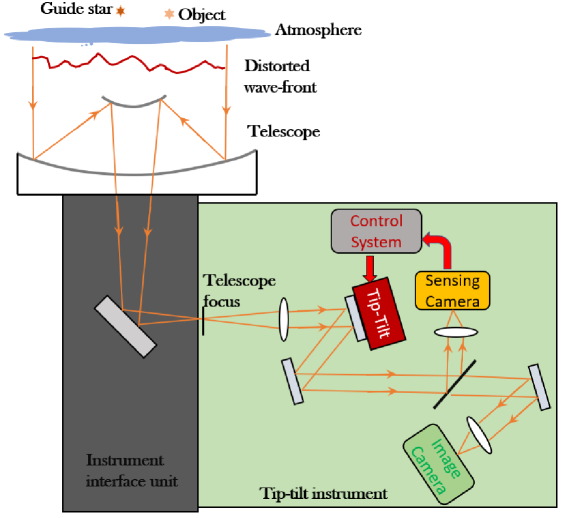
Figure 1: Conceptual layout of a natural guide star tip-tilt correction system. The telescope primary mirror collects the light from a target field. The light beam is directed to tip-tilt instrument. The light is divided between the sensing arm and the imaging arm of the instrument. The image motion is corrected in common path where the tip-tilt stage is placed. The corrected wave-front can be directed to imaging camera or a science instrument.

2 Opto-mechanical design

The tip-tilt system was designed for 1.3 m telescope, Vainu Bappu Observatory located at $78^{\circ}50^{\prime}E$ and $12^{\circ}34^{\prime}N$. The telescope was commissioned in the year 2014. It is a Ritchey-Chretien model telescope with primary and secondary being hyperbolic mirrors. During the routine observations telescope resolution is seeing-limited. A tip-tilt instrument followed by a higher order AO system is envisioned to transform the seeing-limited resolution of the telescope to near diffraction limited case.

2.1 Opto-mechanical design

An optical system of the instrument was designed in ZEMAX ray tracing software. Several design parameters, such as effective focal length, overall weight and dimensions of the instrument were considered. The pixel scale at telescope Cassegrain focus is 0.26^′′/pixel (pixel size = 13 $\mu$m ) while the diffraction limited resolution is 0.106^′′ at 630 nm wavelength. In the optical design of the instrument, the pixel scale was reduced to half of the diffraction limited resolution. This improved the sensitivity of the telescope to measure the image motion. The instrument weighs $\approx$ 28 kg and has dimensions $120\times 60\times 30$ cm³. It was installed on the West port of the telescope as shown in the top panel of Figure 2. A solid model designed in $\it AutoCAD$ is shown in bottom panel of Figure 2. Some key specifications of the telescope and the tip-tilt instrument are listed in Table 1.

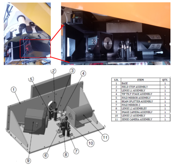
Figure 2: The tip-tilt instrument mounted on the West port of Cassegrain focus of 1.3 m JCB telescope at VBO (top). A CAD model showing the mechanical layout and system components (bottom).

Table 1: Key specifications of tip-tilt instrument. Telescope and instrument layout is shown in Figure 1. F/_#: F-ratio, PS: Pixel Scale.

Property	Value
Wavelength range	480-700 nm
wave-front sense plane FOV2	40′′
Image plane FOV1	1′
Telescope focus F/#, PS	8, 0.26′′
Sensor camera F/#, PS	15.7, 0.06′′
Imaging camera F/#, PS	22.4, 0.08′′

2.2 Sub-components of the instrument

A brief description of essential sub-components of tip-tilt instrument is as follows.

• Tip-tilt stage: We used a fast steering tip-tilt stage from Physik Instrumente (Model: S-330). It is a Piezo-based actuator system with two orthogonal axis. Each of the axis has two actuators that work on the opposite polarity of an applied voltage. These axis are able to deflect the light beam with 0.5 $\mu$rad resolution over a 10 mrad tilt angle. The tip-tilt stage has a one-inch diameter platform to mount a mirror that steers the light beam projected on to it. The stage is driven by Physik Instrumente E-517 control system that has proportional, integral and differential (PID) internal voltage controller to provide a position accuracy of 0.5 $\mu$rad in a close-loop operation.

• Sensing camera: The performance of the tip-tilt instrument depends on its ability to sense the image motion and apply the necessary correction. The sensing camera should be able to operate at high frame rate to record the random drift in the stellar image. We used Andor Neo-sCMOS 2560$\times$2160 pixel, high-speed camera. For exposure time of 1 ms and frame size of $128\times 128$ pixels, we could able to achieve frame rate of $\sim$ 300 using control software developed on LabView platform. With 6.5 $\mu$m pixel size and the magnification achieved by the relay optics, the sensing camera is able to sample the sky with 0.06^′′/pixel.

• Imaging camera: We used Princeton Instruments ProEm eXcelon ($1024\times 1024$, pixel size = $13\mu$m) EMCCD for tilt corrected observations. The CCD is used in continuous exposure mode with simultaneous read out of the data. This is a frame transfer operation. In this mode, the data in active area is vertically shifted to a masked area. This operation takes few microseconds (0.8 $\mu$sec) and enables the active area to be available for next exposure. The full frame of the CCD cover $\approx 1^{\prime}\times 1^{\prime}$ on-sky field of view (FoV) with plate scale of $0.08^{\prime\prime}$/pixel.

2.3 Estimation of image motion

The sensing camera is operated in high-speed mode ($\sim$ 300 fps) to acquire short exposure images. These images were used to estimate the image motion using a centroid tracking method (Close & McCarthy 1994; Golimowski et al. 1992). The noise in the images affects the accuracy of centroid tracking. The images were bias subtracted. Although the magnitude of the dark current itself is negligible, there is considerable bias counts ($\sim$100 counts at 30 K), which contributes error to the centroid estimation. Thus this ‘dark’ subtraction (which includes bias) found to be was essential. The master dark is obtained by taking the median of the dark frames before each experiment.

The centroid estimation should be faster to minimize the time delay between the sensing of the motion and the correction. For this experiment, we have chosen an intensity thresholding centroid technique. In this method, a threshold slightly above the pixel noise level is applied to the image. The method minimizes the noise by assigning zero counts to pixels below the threshold. The resultant image centroid is measured using the weighted average of the intensities as shown in the Equation 1. To measure the improvement in tilt corrected image motion, the root mean square (rms) of the residual centroid motion is estimated using Equation 2:

$$X_{c} = \frac{\sum x_{i}I_{i}}{\sum I_{i}},Y_{c}=\frac{\sum y_{i}I_{i}}{\sum I_{i}},$$ (1)

$$\sigma_{x} = \sqrt[]{\frac{\sum({X_{c}-\bar{X_{c}}})^{2}}{n}},\sigma_{y}=\sqrt[]{\frac{\sum({Y_{c}-\bar{Y_{c}}})^{2}}{n}}$$ (2)

where $X_{c}$, $Y_{c}$ are the estimated centroid of the image, $I_{i,j}$ are pixel intensities, $x_{i,j}$, $y_{i,j}$ are pixel coordinates, $\bar{X_{c}}$, $\bar{Y_{c}}$ are mean centroids and $\sigma_{x}$, $\sigma_{y}$ are associated standard deviations.

2.4 Power spectral density

The power spectral density (PSD) is the measure of energy distributed over a frequency range when the measurements are made within a finite time window (Welch 1967). In this paper, the PSD of the centroids of tilt uncorrected and corrected images was measured. The comparison between the PSD help in determining the correction bandwidth of the tip-tilt instrument. The correction bandwidth is defined as the least frequency at which the ratio of the PSD of the uncorrected and corrected data sets falls to unity, i.e., 0 dB.

$$\widehat{x}(f)=\frac{1}{2\pi\sqrt{T}}\int_{0}^{T}e^{-2{\pi}ift}x(t)dt\\$$ (3)

$$S(f)=|\widehat{x}(f)|^{2}\\$$ (4)

The power spectral density $S(f)$ over limited time interval $[0,T]$ of centroid data $x(t)$ is defined in Equation 3,4. Where, $\widehat{x}(f)$ is the Fourier transform of centroid data with temporal frequency $f$.

2.5 Control Software

A control software with graphical user interface (GUI) is developed using National Instrument’s LabVIEW platform to operate the instrument. The software enables the interoperability between the sensing camera and the tip-tilt stage. The program flow of the control software is shown in the Figure 3. As shown in the flowchart, during the initialization step, the connectivity of the tip-tilt stage and the camera is checked. Subsequently, the exposure time, the number of frames to obtain are set, following which the tip-tilt actuators are initialized. The program has one master loop and one slave loop where the former independently acquires the image frames, and the later processes them in sequence to estimate the centroid. The independence of the master loop from its slave improves the loop frequency of the system. The tip-tilt stage corrects for each of the centroid shifts in real time to compensate for the image motion. There is a time delay of $\approx$ 0.8 ms, after acquiring the image and the tip-tilt mirror reaching its commanded position. The software has option to save the image and centroid data. For optimal performance of the instrument in closed loop, a PID controller was implemented in software.

$$\Delta c(t)=K_{p}e(t)+K_{d}\frac{de(t)}{dt}+K_{i}\int_{0}^{t^{\prime}}e(t^{\prime})dt\\$$ (5)

In the above equation, $K_{p}$, $K_{d}$ and $K_{i}$ are proportional, derivative and integral gains and $e(t)$ is the difference of two consecutive centroid shifts, $\Delta c(t)$ is the centroid shift estimated using the PID control. The controller gains are calculated using trial and error method by monitoring the residual image centroid motion. The estimated values for $K_{p}$, $K_{d}^{\prime}$ and $K_{i}^{\prime}$ are 4E-1, 2.5E-1, 2.3E-3 respectively. Here, $K_{d}^{\prime}$ and $K_{i}^{\prime}$ are $K_{d}*T$ and $K_{i}/T$, where $T$ is time interval between two consecutive centroids. The $\Delta c(t)$ is multiplied by voltage required to cause a pixel shift.

Figure 3: Flow chart of control software.

2.6 Instrument calibration

The calibration is required to accurately map the image wandering on the CCD to the input control voltage that drives the piezo actuators to compensate the image movement across the detector plane. This mapping is unique for each instrument as the linear beam-throw by steering mirror depends on the specific layout of the optical components.

The axis of the stage have been centred around its maximum dynamic range i.e. at five mrad. The layout of laboratory setup is shown in the Figure 4. A point source is generated by spatially filtering the laser beam as shown in the figure. The spatial filter consists of a microscope objective and a Pinhole of 10 $\mu$m. For performance analysis, the centroid motion of the point source image on sensing camera has been observed.

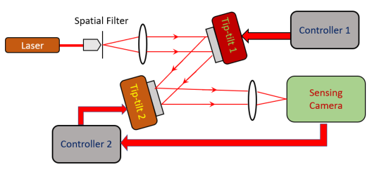
Figure 4: Experiment layout for the tip-tilt calibration in the lab. The tip-tilt stage TT1 was used to induce the image motion while TT2 was used to correct it. The CCD camera was used for recording the movement of the laser spot.

2.6.1 Axis alignment

Ideally, the movement of two actuator axis should be perfectly aligned with the pixel rows (horizontal) and columns (vertical) of the CCD. Initially, the axis of the tip-tilt stage were coarsely aligned by observing the spot traces in the live camera images. After making the fine adjustments, a residual deviation in alignment was measured by taking multiple images of the source on CCD while the beam was progressively steered (horizontally or vertically) in a sequence of voltage steps applied to individual actuators, one at a time. Furthermore, to minimize the alignment error, a rotation matrix (Russell 1971) as shown in Equation 6 was generated from the obtained data. To compensate the small offset in the alignment the shift in the image motion is multiplied with this matrix before applying the corrections in real-time.

$$\begin{bmatrix}x^{\prime}\\ y^{\prime}\\ \end{bmatrix}=\begin{bmatrix}a&b\\ c&d\\ \end{bmatrix}*\begin{bmatrix}x\\ y\\ \end{bmatrix}\\$$ (6)

$$X^{\prime}=AX\\$$ (7)

$$V=KX^{\prime}\\$$ (8)

Equation 7 is the relation between the rotation matrix $A$ and the centroid shifts. In the Equation 6, $x$ and $y$ are image centroid shift, $x^{\prime}$ and $y^{\prime}$ are centroid shift after rotation along H-axis and V-axis. In our experiment, the measured elements of the rotation matrix ($A$) were: $a=1.003$,$b=0.0013$, $c=0.0015$ and $d=0.9996$. These are typical values for a closely aligned system. In Equation 8, $V$ is voltage applied to tip-tilt stage and $K$ is the voltage per unit shift in the centroid.

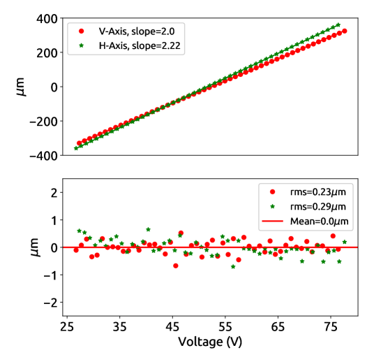
Figure 5: Calibration curves for two-axis tip-tilt stage. The horizontal (H-axis), vertical (V-axis) have been moved with equal step size of 1 V (top). In both cases, the rms deviation from the linear fit is $\sim$ 0.3 $\mu$m (bottom).

The response of each actuator is tested independently by tilting it over a range of 3 mrad to 8 mrad with an input voltage step size of 1V. The image centroids for each input step voltage is recorded. The mean centroid shift is estimated by measuring the average difference between two consecutive centroids over the earlier mentioned tilt range. Figure 5 (top panel) shows the image centroid shift on the camera as a function of input voltage. The error in actuator movement is defined as the difference between two consecutive centroids with respect to the mean centroid shift. It is plotted in the Figure 5 (bottom panel). The estimated rms error in the actuator movement is less than 0.3 $\mu$m. Results of tip-tilt stage calibration are summarized in Table 2.

Table 2: Tip-tilt stage axis calibration

Parameter	Value
Number of samples	51
Exposure time per sample	3 ms
Tip-Tilt range	3-8 mrad
Voltage range	24-78 V
Voltage step size	$\sim$ 1V
Linear image shift (total)	$\sim$650 $\mu$m
Mean centroid shift	$\sim$ 12 $\mu$m
rms error in movement	$\sim$ 0.3$\mu$m

3 Laboratory testing of the instrument

Initially, a prototype of the instrument was set up in the laboratory. Centroid data of short exposure images of the star was obtained a priory from the telescope. This data was then used as input to one of the steering mirrors to simulate the image motion in the lab studies. For characterization of the instrument, the residual image centroid motion and the PSD of tilt uncorrected and corrected images were analysed.

The layout of the laboratory setup is shown in Figure 4. In this study we used two tip-tilt stages -one to induce the image motion (Piezosystems jena, Model Number: PSH x/2); and the other to correct it. The former has the frequency response up to 3 kHz, 0.02 $\mu$rad resolution and $\pm$4 mrad dynamic range.

The centroid data (in pixels) need to be converted to the voltages which will be applied to the tip-tilt stage 1 (TT1). For this purpose, the per-pixel voltage (0.21 V for H-axis and 0.23 V for V-axis) is estimated for the TT1 system from the calibration curves. The voltages were applied to TT1 to induce the image motion at the frequency of 33 Hz. This is to maintain at least 10 times correction bandwidth (Hardy 1998) of the system. The induced image motion is tracked using the centroid estimations.

The image motion data was recorded both with and without the tip-tilt correction. The Figure 6 shows the image centroid motion in the laboratory. The rms of corrected image motion is reduced by a factor of $\sim$ 12.8 in horizontal axis and $\sim$ 9.8 in vertical axis, compared to the uncorrected.

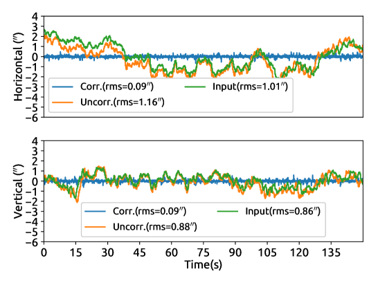
Figure 6: Image centroid motion in arcsec (^′′) along horizontal (top panel) and vertical (bottom panel) axis of the camera. The plot has three sets of data i.e. the induced image motion, the uncorrected image motion and the corrected residual image motion. The induced and the sensed image motion has $\sim$ $96\%$ correlation. The image shift is converted to arc-seconds by multiplying the image shift with pixel scale similar to the telescope (0.06^′′).

The closed loop correction bandwidth of the system was estimated from the power spectral densities of the image motions for both tilt uncorrected and corrected cases. The observed correction bandwidth (0 dB)is $\sim 25Hz$.

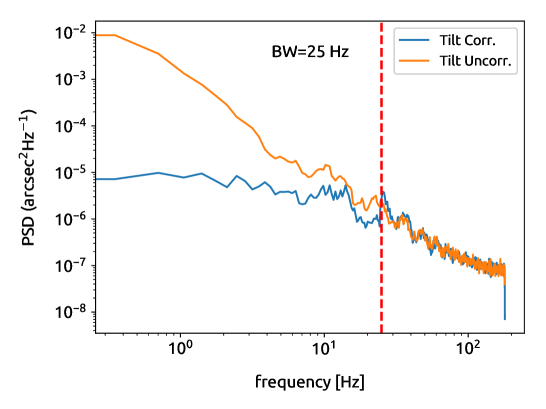
Figure 7: The power spectral density of centroid data in laboratory. The vertical line signifies the merging of the two plots. This is the 0 dB closed loop correction bandwidth (red line) of the system.

4 On-sky testing of the instrument

After successful alignment and calibration, the instrument was mounted on the telescope (see Figure 2). Initial tests were done in March 2018. The on-sky performance of the tip-tilt system is described in terms of the residual rms image motion, correction bandwidth, full width half maximum and peak intensity of the image. We are presenting these results after satisfactory performance has been achieved since January 2019.

4.1 Observations

The objects of $m_{v}$ brighter than six have been chosen. These objects were close to the zenith with hour angle of less than one hour. Preferably, targets with more than one object in the field have been chosen. This enables the instrument to sense the bright star with high-speed and apply the correction to the entire field. List of the targets used is given in the Table 3. These targets were observed on different days from March 2019 to May 2019.

For high speed performance, a region of interest (ROI) has been chosen around the target image on sensing camera. This enhanced the frame rate and thus increased the overall loop frequency. The exposure times are chosen from 3 ms to 20 ms. The longer exposure time allows us to observe the relatively fainter targets. This enables us to vary a loop frequency from $\sim$ 290 fps to 47 fps. Each data set was recorded over 150 seconds. Under poor atmospheric conditions, the binning operation was carried out in the program to enhance the signal to noise ratio. This might have reduced the accuracy in centroid estimation, but overall, it improved the correction performance.

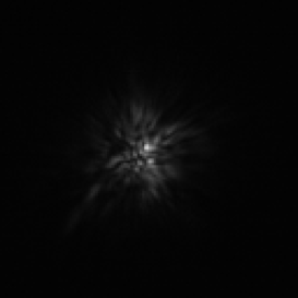
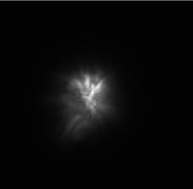
Figure 8: Illustration object: HIP57632. The short exposure time (3 ms) image on sensing camera (left). Relatively long exposure time (200 ms) image on the imaging camera. The frame size is $\sim$ $10^{\prime\prime}\times 10^{\prime\prime}$.

The tilt corrected images were acquired on imaging camera. This camera was given relatively longer exposure time($\sim$200 ms). Because of a set of objects with different magnitude, we chose a fixed exposure time to avoid pixel saturation in case of a brighter object. In Figure 8, the short exposure image of sensing camera and the imaging camera were shown.

A total of 1000 images of each target field were acquired on the imaging camera. Every target was observed for tilt uncorrected and corrected images. These images were processed using a Python script. The image frames have been dark subtracted and flat fielded prior to the analysis. The co-added images, as shown in Figure 9, will give the equivalently long exposure images. Finally, these images were divided by number of obtained frames. This will average the intensity of each frame and minimize the effect of intensity fluctuations on the estimation of the performance.

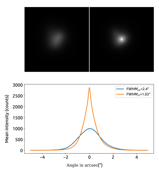
Figure 9: Illustration: Object HIP57632. The tilt uncorrected (top-left) and the tilt corrected (top-right) co-added images. The psf of the image along the horizontal axis is shown in the bottom panel.

4.2 Image centroid, PSD and psf comparison

The instrument was characterized by measuring the residual image motion. Figure 10 shows the tilt-corrected and uncorrected image centroids recorded consecutively by sensing camera. The rms value was reduced to $\sim$0.08^′′ from $\sim$1.26^′′.

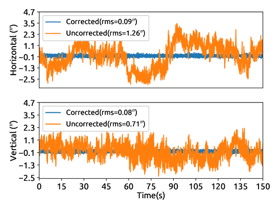
Figure 10: Image centroid motion of HIP57632. The rms image motion has been reduced by a factor of $\sim$ 14 in horizontal axis and $\sim$ 8.9 in vertical axis.

The image motion power spectral density is shown in Figure 11. The correction bandwidth of the system is found to be $\sim$26 Hz, depicted with a vertical line in the figure. The temporal frequencies beyond this limit are uncorrected.

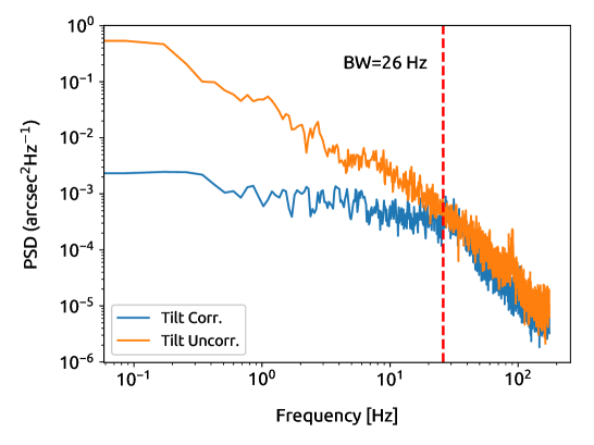
Figure 11: The power spectral density of the image motion for star HIP57632. Vertical dotted line demarcates the close-loop bandwidth of the system.

On imaging camera, the psf is expected to be sharper with tip-tilt instrument in operation. The Figure 9 shows the psf of HIP57632. The full width at half maximum (FWHM) of the psf has improved from 2.4^′′ to 1.03^′′. The improvement in FWHM was calculated as shown in Equation 9. This is a $\sim$ 57% improvement.

$$Improvement(\%)=\frac{FWHM_{uc}-FWHM_{cr}}{FWHM_{uc}}\times 100\\$$ (9)

Here, $FWHM_{uc}$ is for uncorrected image and $FHWM_{cr}$ is for corrected image.

In the above case, the peak intensity of tilt corrected psf has increased by factor of $\sim$ 2.8. This improves the sensitivity of the instrument towards the observation of a fainter object. The sensitivity was estimated by using the Equation 10. This is equation relates the magnitude difference of a star with peak intensity of the tilt uncorrected and corrected images. It is observed that the sensitivity is improved by a factor of 1.1 in magnitude.

$$\Delta m_{v}=-2.512*log_{10}\Big{[}\frac{I_{c}}{I_{uc}}\Big{]}\\$$ (10)

Where, ${I_{c}}/{I_{uc}}$ is the ratio of peak intensities of tilt corrected and uncorrected images, $\Delta m_{v}$ is the improvement in apparent magnitude. Here, we considered, ${I_{c}}/{I_{uc}}$ as ${4.3}/{1.49}$.

4.3 Effect of loop frequency

The optimal frame rate is essential for the effective tilt correction of the images in a close-loop operation. This is in confirmation with the fact that the wave-front distortions are caused by the spatial and the temporal disturbances in the atmosphere. The spatial distortions are corrected by compensating for the shift in the image centroid. But the dynamic nature of the atmosphere induces high frequency image motion. To overcome this effect, the time delay between the instant of estimation of the shifts and the instant of the correction applied to the corrector should be kept minimum.

To study the effect of loop frequency on the peak intensity of the tilt-corrected images, we observed HIP57632 with different frame rates. The frame rate was changed by changing the exposure time of the sensing camera from three to 20 ms, yielding loop frequencies of 290 to 47 Hz.

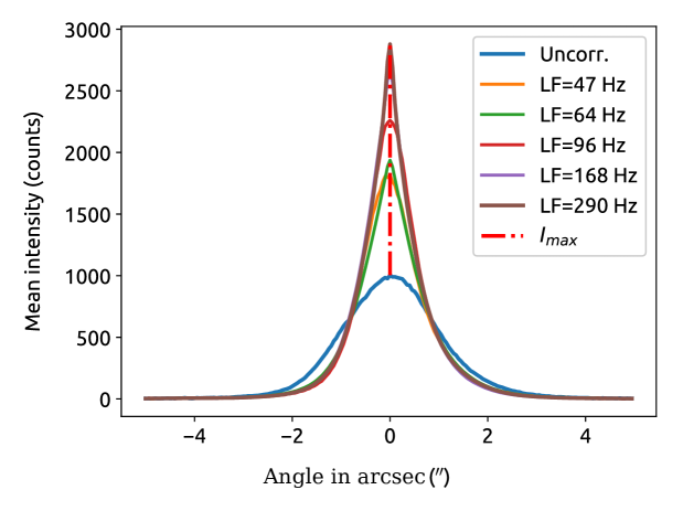
Figure 12: Comparison of tip-tilt corrected psf of HIP57632 for different loop frequencies. The peak intensity is showing logistic growth with loop frequency.

In Figure 12, cross section of the psfs with different loop frequency are plotted. The peak intensity of the psf was increased with increase in loop frequency and the result is plotted in Figure 13. In this figure, the peak factor was defined as the ratio of peak intensity of the tilt corrected to that of uncorrected image.

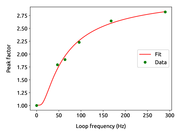
Figure 13: Increment in peak factor with loop frequency.

We have modeled the effect of loop frequency on peak factor with a function of the form shown in Equation 11.

$$I_{pf}(f)=K_{1}+K_{2}*(1-e^{-f_{0}/f})\\$$ (11)

In the above equation, $f$ is loop frequency, $I_{pf}$ is peak factor and the estimated constants are $K_{1}$, $K_{2}$ and $f_{0}$ estimated to be $\approx$ 3.2, -2.2 and 52 Hz, respectively. The units of $K_{2}$ and $K_{1}$ are similar to $I_{max}$. Arguably, the estimated values of the constants depend on the target intensity and the atmospheric seeing conditions.

In Figure 14, the power spectral densities for different loop frequencies are shown. We can see that that the correction bandwidth increased to $\sim$ 26 Hz at 290 Hz from $\sim$ 4.8 Hz at 47 Hz loop frequency. On an average, the correction bandwidth is $\sim$ 1/10 of the loop frequency which is in agreement with other studies reported in literature (Hardy 1998).

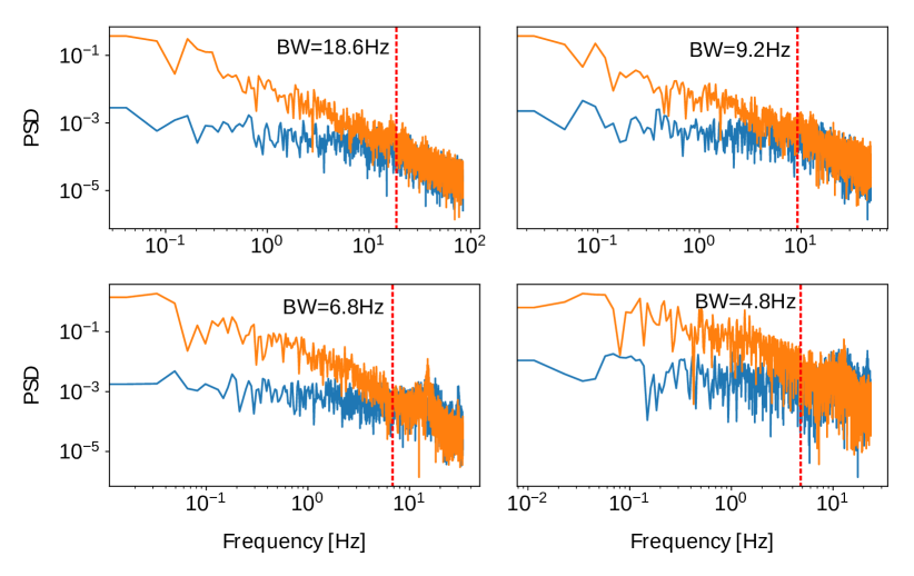
Figure 14: The PSD (arcsec²Hz^-1) with respect to correction bandwidth for object HIP57632. The orange and the blue lines are PSD of tilt uncorrected and corrected centroid data. The loop frequency is 168 Hz (left) and 96 Hz (right) for top row, 64 Hz (left) and 47 Hz (right) for bottom row and their correction bandwidths (red line) are in the plot.

4.4 Gain in angular resolution

The tilt corrected images show improvement in angular resolution. The gain in angular resolution is a function of relative sizes of the telescope aperture (D) and the atmospheric coherence diameter $r_{0}$. This relation can be theoretically estimated using the formalism given by Roddier (1981) and is shown in Figure 15. The gain is defined as the ratio of equivalent width (Roddier 1981) of tilt uncorrected image and corrected images. The observed values of the gain for a set of six targets as listed in Table 3 are over plotted on the theoretical curve. $r_{0}$ is estimated from the equivalent width of the uncorrected images (to get the $D/r_{0}$ for the observed data). The observed gain has shown a deviation up to 24% from the theoretical gain.

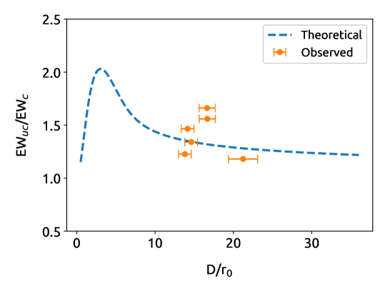
Figure 15: Comparison of gain in angular resolution between the theoretical and the observed data. On vertical axis, EW_uc and EW_c are equivalent widths of tilt uncorrected and corrected image.

4.5 Performance of the instrument on faint targets

We observed a set of seven objects as listed in Table 3 (objects 7-13) to validate the increase in sensitivity of the instrument due to image stabilization. Usually, a bright star near faint star is used for sensing the image motions and the same correction is applied to the entire field. If the faint star is close enough, the corrections are similar and thus the sensitivity of the instrument on the faint star increases.

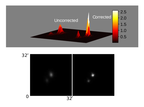
Figure 16: Surface plot of HIP50583, containing average tilt uncorrected and corrected image. The frame size is $\sim$ $32^{\prime\prime}\times 32^{\prime\prime}$.

In Figure 16 the tilt uncorrected and corrected image of HIP50583 is shown. The object has brightness of 2.37 in magnitude with a relatively fainter object with magnitude of 3.47, at an angular separation of 4.63^′′. The correction increased the peak intensity by a factor of $\sim$ 2.5 times in brighter object $\sim$ 2.1 times in fainter object. The angular resolution (FWHM) of these objects improved by 52% and 46% respectively. Similar to this, several other objects were observed and these results are shown in Figure 17 and Table 3.

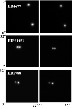
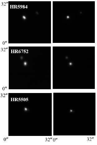
Figure 17: Examples: Tilt uncorrected and corrected images of various targets.

Table 3: List of observed stars with varying angular separation. In the table, $m_{v}$ is apparent magnitude, $\Delta m_{v}$ is magnitude different between two objects and ’Sep’ is angular separation between the objects in arc-sec. Peak factor is the ratio of tilt corrected and uncorrected image and improvement in resolution ($R$) is similar to Equation 9. LF is approximate loop frequency

Sl.No.	Target	RA	Dec	$m_{v}$	$\Delta m_{v}$	Sep(${\prime\prime}$)	LF (fps)	Peak factor	R(%)
1	HIP57632,$\--$	11 49 03.5	+14 34 19.4	2.13	$\--$	$\--$	290	2.8,$\--$	57,$\--$
2	HIP54879,$\--$	11 14 14.4	+15 25 46.4	3.35	$\--$	$\--$	290	2.1,$\--$	45,$\--$
3	HIP37279,$\--$	07 39 18.1	+05 13 29.9	0.37	$\--$	$\--$	290	1.8,$\--$	44,$\--$
4	HIP65474,$\--$	13 25 11.5	-11 09 40.7	0.97	$\--$	$\--$	290	1.4,$\--$	32,$\--$
5	HIP67927,$\--$	13 54 41.0	+18 23 51.7	2.68	$\--$	$\--$	290	1.5,$\--$	38,$\--$
6	HIP69673,$\--$	14 15 39.6	+19 10 56.6	-0.05	$\--$	$\--$	290	2.4,$\--$	50,$\--$
7	HIP50583, gam02 Leo	10 19 58	19 50 29.3	2.37	1.1	4.63	290	2.5, 2.1	52, 46
8	HIP61941, gam Vir B	12 41 39.6	-01 26 57.7	2.74	0.75	1.52	290	2.4, 2.3	51, 49
9	HR4677, HD 106976	12 18 08	-03 57 05.01	5.99	0.7	20.33	64	1.5, 1.3	36, 32
10	HR6752, 70 Oph B	18 05 27	02 30 0.0	4.03	2.04	4.91	98	1.9, 1.7	41,36
11	HR5789, del Ser B	15 34 48.1	10 32 15.9	3.79	1.4	4.1	98	1.7, 1.5	32, 33
12	HR5984, bet02 Sco	16 05 26.2	-19 48 19.6	2.5	2.3	13.64	98	1.8, 1.6	42, 36
13	HR5505, eps Boo B	14 44 59.2	+27 04 27.2	2.39	2.4	2.58	98	1.8, 1.5	43, 31

5 Summary and conclusion

A tip-tilt instrument has been developed for the 1.3 m JCB telescope to overcome the image degradation caused by angle of arrival fluctuations. In laboratory, a simulated image motion corresponding the actual data acquired from the telescope was used to characterize the instrument. The on-sky performance of the instrument was analyzed by observing several stars of varying brightness and angular separation. The real-time correction has shown a characteristic improvement in the image quality that is consistent with previously reported studies in the literature. This study has led to the following findings and conclusions:

1. In laboratory, the rms image motion was reduced by $\sim$12 times and the correction bandwidth was estimated to be a $\sim$ 25 Hz for a loop frequency of 290 Hz.

2. On telescope, the rms image motion was reduced by $\sim$14 times and the correction bandwidth was estimated to be about 0.1 times the loop frequency, where the loop frequency was varied from 47 Hz to 290 Hz (five distinct frequencies in this range).

3. The FWHM of the image reduced from 2.4^′′ to 1.03^′′. This corresponds to 57% improvement in the image resolution.

4. The sensitivity of the instrument was found to increased by a factor of 1.1 magnitude (corresponding to the increase in the dynamic range, peak intensity ratio of 2.8).

5. In the case of targets with two close-by stars in the field, the FWHM of the individual psf decreased and the peak brightness increased depending on the magnitudes. For example, in the case of HIP50583 with separation of 4.63^′′ and magnitude difference of 1.1, the FWHM of the bright star increased by 52% and that of the faint star increased by 46%. The peak brightness of the bright star increased by a factor of $\sim$ 2.5 and that of the faint star increased by a factor of $\sim$ 2.1.

To further improve the image quality to near diffraction limited resolution of the telescope, the work on a higher order AO system is under progress.

References

- Close & McCarthy (1994) Close, L., & McCarthy, D. 1994, Publications of the Astronomical Society of the Pacific, 106, 77
- Dainty et al. (1998) Dainty, J. C., Koryabin, A. V., & Kudryashov, A. V. 1998, Applied optics, 37, 4663
- Davis & Tango (1996) Davis, J., & Tango, W. 1996, PASP, 108, 456
- Eaton et al. (1985) Eaton, F., Peterson, W., Hines, J., & Fernandez, G. 1985, Applied optics, 24, 3264
- Fried (1965) Fried, D. L. 1965, J. Opt. Soc. Am. A, 55, 1427
- Fried (1966a) Fried, D. L. 1966a, J. Opt. Soc. Am. A, 56, 1372
- Fried (1966b) Fried, D. L. 1966b, J. Opt. Soc. Am. A, 56, 1372
- Glindemann (1997) Glindemann, A. 1997, Publications of the Astronomical Society of the Pacific, 109, 682
- Glindemann et al. (1997) Glindemann, A., McCaughrean, M. J., Hippler, S., et al. 1997, Publications of the Astronomical Society of the Pacific, 109, 688
- Golimowski et al. (1992) Golimowski, D., Clampin, M., Durrance, S., & Barkhouser, R. 1992, Applied optics, 31, 4405
- Greenwood (1977) Greenwood, D. P. 1977, JOSA, 67, 390
- Hardy (1998) Hardy, J. W. 1998, Adaptive Optics for Astronomical Telescopes (Oxford.Univ.press), 448
- Hubbard et al. (1979) Hubbard, G., Hege, K., Reed, M., et al. 1979, The Astronomical Journal, 84, 1437
- Kellerer & Tokovinin (2007) Kellerer, A., & Tokovinin, A. 2007, A&A, 461, 775
- Martin (1987) Martin, H. M. 1987, PASP, 99, 1360
- Max et al. (1997) Max, C. E., Olivier, S. S., Friedman, H. W., et al. 1997, Science, 277, 1649
- Noll (1976) Noll, R. J. 1976, JOSA, 66, 207
- Racine & McClure (1989) Racine, R., & McClure, R. D. 1989, Publications of the Astronomical Society of the Pacific, 101, 731
- Roddier (1981) Roddier, F. 1981, in Progress in optics, Vol. 19 (Elsevier), 281
- Rousset et al. (1990) Rousset, G., Fontanella, J., Kern, P., Gigan, P., & Rigaut, F. 1990, Astronomy and Astrophysics, 230, L29
- Russell (1971) Russell, C. T. 1971, Cosmic Electrodynamics, 2, 184
- Sarazin & Tokovinin (2002) Sarazin, M., & Tokovinin, A. 2002, in European Southern Observatory Conference and Workshop Proceedings, Vol. 58, 321
- Sreekanth et al. (2019) Sreekanth, R. V., Banyal, R. K., Sridharan, R., & Selvaraj, A. 2019, Research in Astronomy and Astrophysics, 19, 074
- Welch (1967) Welch, P. 1967, IEEE Transactions on audio and electroacoustics, 15, 70
- Wizinowich et al. (2000) Wizinowich, P. L., Acton, D. S., Lai, O., et al. 2000, in Adaptive Optical Systems Technology, Vol. 4007, International Society for Optics and Photonics, 2