WUB/19-04

Constrained Hybrid Monte Carlo algorithms for gauge-Higgs models

Abstract

We develop Hybrid Monte Carlo (HMC) algorithms for constrained Hamiltonian systems of gauge-Higgs models and introduce a new observable for the constraint effective Higgs potential. We use an extension of the so-called Rattle algorithm to general Hamiltonians for constrained systems, which we adapt to the 4D Abelian-Higgs model and the 5D SU(2) gauge theory on the torus and on the orbifold. The derivative of the potential is measured via the expectation value of the Lagrange multiplier for the constraint condition and allows a much more precise determination of the effective potential than conventional histogram methods. With the new method, we can access the potential over the full domain of the Higgs variable, while the histogram method is restricted to a short region around the expectation value of the Higgs field in unconstrained simulations, and the statistical precision does not deteriorate when the volume is increased. We further verify our results by comparing to the one-loop Higgs potential of the 4D Abelian-Higgs model in unitary gauge and find good agreement. To our knowledge, this is the first time this problem has been addressed for theories with gauge fields. The algorithm can also be used in four dimensions to study finite temperature and density transitions via effective Polyakov loop actions.

1 INTRODUCTION

The Brout-Englert-Higgs (BEH) mechanism [1, 2] explains the generation of the mass of gauge bosons in gauge theories coupled to a scalar field called the Higgs field. The Standard Model (SM) of particle physics relies on this mechanism. In 2012 a scalar particle of mass around $125$ GeV was discovered at the LHC accelerator at CERN [3, 4] rendering the SM complete. The masses of the gauge bosons arise by Spontaneous Symmetry Breaking (SSB) triggered by the Higgs potential. The origin of the Higgs potential is, as of yet, unknown. Moreover, the mass of the Higgs particle has a quadratic sensitivity to a ultra-violet cut-off, the so-called hierarchy problem. These problems suggest that a more fundamental process is behind the Higgs mechanism.

An elegant solution is provided by Gauge-Higgs Unification (GHU) models [5, 6, 7] and relies on the existence of extra dimensions. In these models the Higgs field is identified with (some of) the extra-dimensional components of the gauge field. The gauge symmetry of the higher dimensional theory protects the Higgs mass from corrections which are quadratic in the cut-off. Moreover, a Higgs potential is generated by loop effects and can give a mass to the gauge bosons in the regular four dimensions. A particular GHU model in terms of a five-dimensional (5D) SU(2) gauge theory where the extra dimension is compactified on an $S^{1}/\mathbb{Z}_{2}$ orbifold was formulated in [8, 9] in the context of lattice field theory. At the fixed points of the orbifold, the gauge group is explicitly broken down to U(1). The theory exhibits SSB [10, 11] in accordance with Elitzur’s theorem [12], via the spontaneous breaking of the so-called stick symmetry [13, 14], giving rise to the BEH mechanism. This observation was confirmed in [15, 16] via semi-analytic mean-field calculations.

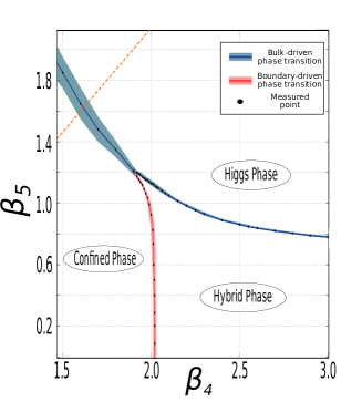
The system has been found to exhibit three phases, see Fig. 1 (left), separated by first order phase transition lines which are characterized by the expectation value of the Polyakov loop in the extra dimension: in the confined (de-confined) phase the Polyakov loop exhibit zero (non-zero) expectation value in every direction. In this context, the de-confined phase is labelled Higgs phase, because it is where the Higgs potential develops SSB, giving rise to non-zero gauge boson masses. The third phase, which is characteristic only of the orbifold geometry, shows confined dynamics in the orbifold’s bulk, and de-confined dynamics on its boundaries; it is, therefore, called hybrid phase. These results, which are favorably pointing towards the suitability of this theory for describing the electro-weak sector of the Standard Model, are reported in [17, 18].

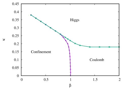
Figure 1: (left) From [17]. The phase diagram for $N_{5}=4$ in the region of the Higgs-hybrid phase transition of the 5D orbifold gauge theory (see Sect. 5). The points show the location of a first-order phase transition. The red and blue lines represent the width of the corresponding hystereses, while the dashed orange line represents $\gamma=1$ ($\beta_{4}=\beta_{5}$). (right) The phase diagram of the Abelian-Higgs model (see Sect. 3) with $\lambda=1$ showing a similar phase structure. The green and purple curves correspond to different order parameters.

The phase structure is similar to the one of the four-dimensional (4D) Abelian-Higgs model, shown in Fig. 1 (right). Moreover, on the orbifold boundaries of the 5D GHU model one observes dimensional reduction from five to four dimensions [17], which suggests that there is a localization mechanism for the gauge field. In order to corroborate the relation of the 5D GHU model with torus and orbifold boundary conditions to the dimensionally reduced theory, the 4D adjoint resp. Abelian-Higgs model, we want to compute the effective potentials in the various cases.

The goal of this work is to develop an algorithm for measuring the so-called constraint effective potential in lattice simulations of gauge-Higgs models. The constraint effective potential corresponds in the infinite volume limit to the conventional effective potential [19, 20]. A way to measure the constraint effective potential is presented in Ref. [21]. It is based on the Hybrid Monte Carlo (HMC) algorithm [22] for constrained Hamiltonians. The latter include constraint conditions on the Higgs fields which lead to the constrained equations of motion. This is discussed in Sect. 2 where we derive a formula to measure the derivative of the constraint effective potential in terms of the expectation value of the Lagrange multiplier for the constraint. Then we focus on the implementation of the constrained HMC for the 4D Abelian-Higgs model Sect. 3 and the 5D SU(2) gauge theory with torus Sect. 4 and orbifold Sect. 5 boundary conditions, and present constraint effective potentials for all cases. In Sect. 3.3 we compare the constraint effective potential of the 4D Abelian-Higgs model in unitary gauge to the one-loop (continuum) effective potential for this model [23]. In the conclusions Sect. 6 we give an outlook to the application of our constrained algorithms to measure effective potentials in gauge-Higgs models and also in other theories, e.g., in finite temperature Quantum Chromodynamics (QCD).

2 THE CONSTRAINT EFFECTIVE POTENTIAL

The exact effective potential is the infinite volume limit of the so-called constraint potential $U_{\Omega}(\Phi)\overset{\Omega\rightarrow\infty}{\rightarrow}U_{{\rm eff}}(\Phi)$ [19, 20]. The latter can be calculated non-perturbatively, via simulating the constrained path integral,

$$e^{-\Omega U_{\Omega}(\Phi)}=\int\mathcal{D}\phi\delta(\frac{1}{\Omega}\sum_{n_{\mu}}\mathcal{H}(n_{\mu})-\Phi)e^{-S[\phi]}$$ (2.1)

where $n_{\mu}$ ($\mu=0,1,2,3$) are the integer coordinates of the points on a lattice with volume $\Omega$ and the average of the Higgs field $\mathcal{H}(n_{\mu})$, constructed from the field variables $\phi(n_{\mu})$, takes a fixed value $\Phi$. This was first shown in the pure Higgs theory by Kuti and Shen [21], who suggested to measure the derivative of the constraint effective potential $U_{\Omega}$ with respect to the constraint field $\Phi$ during the constrained simulations. This method requires a separate simulation for every value of $\Phi$, but the effective potential can be determined with greater accuracy than fitting a distribution $P(\Phi)$ from unconstrained simulations. In order to derive $U_{\Omega}(\Phi)$ we introduce the constrained Hamiltonian

$$\tilde{H}[\phi,\pi] = H[\phi,\pi]+\lambda^{(1)}\biggr{(}\frac{1}{\Omega}\sum_{n_{\mu}}\mathcal{H}(n_{\mu})-\Phi\biggr{)},\quad H[\phi,\pi]=S[\phi]+\frac{1}{2}\sum_{n_{\mu}}\pi^{2}(n_{\mu})$$ (2.2)

with fictitious momentum variables $\pi(n_{\mu})$, including the Lagrange multiplier $\lambda^{(1)}$, to be determined in such a way that it ensures the constraint condition, which demands that the Higgs field $\mathcal{H}(n_{\mu})$ fluctuates around a fixed average value $\Phi$. Using the constrained Hamiltonian (2.2) we rewrite the constrained path integral (2.1) as

$$e^{-\Omega U_{\Omega}(\Phi)} = \int\mathcal{D}\phi\delta(\frac{1}{\Omega}\sum_{n_{\mu}}\mathcal{H}(n_{\mu})-\Phi)e^{-S[\phi]}=\int\mathcal{D}\phi\mathcal{D}\pi e^{-\tilde{H}[\phi,\pi]}$$ (2.3)

The derivative of Eq. (2.3) with respect to the constrained variable $\Phi$ yields

$$-\Omega U_{\Omega}^{\prime}e^{-\Omega U_{\Omega}} = -\int\mathcal{D}\phi\mathcal{D}\pi\tilde{H}^{\prime}e^{-\tilde{H}}=\int\mathcal{D}\phi\mathcal{D}\pi\lambda^{(1)}e^{-\tilde{H}}$$ (2.4)

$$\Rightarrow U_{\Omega}^{\prime}(\Phi) = -\dfrac{1}{\Omega}\dfrac{\int\mathcal{D}\phi\mathcal{D}\pi\lambda^{(1)}e^{-\tilde{H}}}{e^{-\Omega U_{\Omega}}}=-\dfrac{1}{\Omega}\big{\langle}\lambda^{(1)}\big{\rangle}_{\Phi}\equiv U_{\Omega,\rm{cnst.}}^{\prime}$$ (2.5)

the derivative of the constraint effective potential $U_{\Omega}^{\prime}(\Phi)\equiv U_{\Omega,\rm{cnst.}}^{\prime}$ given by the expectation value of the first Lagrange multiplier during simulations at fixed $\Phi$ ($\langle\ldots\rangle_{\Phi}$).

The simulations are performed using Hybrid Monte Carlo methods [22] implementing constrained equations of motion (cEOMs) of the form

$$\dot{\phi}(n_{\mu}) = \dfrac{\partial\tilde{H}}{\partial\pi(n_{\mu})}=\pi(n_{\mu})\quad\mbox{and}\quad\dot{\pi}(n_{\mu})=-\dfrac{\partial\tilde{H}}{\partial\phi(n_{\mu})}=-\dfrac{\partial S}{\partial\phi(n_{\mu})}-\dfrac{\lambda^{(1)}}{\Omega}\dfrac{\partial\mathcal{H}}{\partial\phi(n_{\mu})},$$ (2.6)

including a term incorporating the Lagrange multiplier, which has to be evaluated first, before solving the cEOMs. This is done by demanding that the first derivative of the constraint condition with respect to molecular dynamics time, the so-called hidden constraint, vanishes as the constraint is a conserved quantity. For a non-composite Higgs field $\mathcal{H}(n_{\mu})$ we have a constraint condition that is linear in the underlying fields and the hidden constraint only depends on the momenta $\pi(n_{\mu})$. In this case we can apply standard leap-frog algorithms, which preserve linear constraints exactly, as all Runge-Kutta schemes. If the constraint is applied to composite fields however, e.g., $\mathcal{H}(n_{\mu})=\phi^{\dagger}(n_{\mu})\phi(n_{\mu})$ as in the Abelian-Higgs model, we get additional conditions of the form $\sum_{n_{\mu}}\dot{\phi}(n_{\mu})\phi(n_{\mu})=\sum_{n_{\mu}}\pi(n_{\mu})\phi(n_{\mu})$, depending on $\pi(n_{\mu})$ and $\phi(n_{\mu})$. In standard leap-frog algorithms, these fields are never defined at the same integration time in a trajectory, which spoils the evaluation of the hidden constraint. In the case of SU(N) gauge fields, the situation is even worse. First of all, the definition of a gauge invariant Higgs field leads to composite fields in terms of the underlying gauge variables. Further, the equations of motion define the change of the fields in HMC algorithms not by an additive but a multiplicative exponential term proportional to the momenta $\pi(n_{\mu})$, which causes an additional challenge for the determination of the Lagrange multiplier(s), cf. sections 4 and 5 and appendices A.2-A.4.

We use an extension of the Newton-Störmer-Verlet-leapfrog method, the so-called Rattle algorithm for general Hamiltonians of constrained systems [24, 25], with an additional half integration step for the momenta $\pi$ ($\pi_{n+1/2}$ to $\pi_{n+1}$, the index $n$ denotes the molecular dynamics time step $nh$, with the integration step size $h$). This ensures to have field and momentum variables at the same integration time and allows us to apply the hidden constraint. The implementations of the constrained equations of motion for our special cases using the Rattle algorithm are detailed in appendix A. In the next chapters we summarize the new algorithms for the various models with numerical tests of their time-reversibility. Further, we present first results for the constraint effective potentials and compare them to Higgs potentials from unconstrained simulations using the histogram method and a one-loop Higgs potential [23].

3 4D ABELIAN-HIGGS MODEL

The action of the 4D Abelian-Higgs model is given by

$$S[U_{\mu},\phi] = S_{g}[U_{\mu}]+S_{\phi}[U_{\mu},\phi],\quad S_{g}[U]=\beta\sum_{n_{\mu}}\sum_{\mu<\nu}\left\{1-\mbox{Re}U_{\mu\nu}(n_{\mu})\right\}$$ (3.1)

$$S_{\phi}[U_{\mu},\phi] = \sum_{n_{\mu}}|\phi(n_{\mu})|^{2}-2\kappa\sum_{\mu}\mbox{Re}\left\{\phi^{\dagger}(n_{\mu})[U_{\mu}(n_{\mu})]^{q}\phi(n_{\mu}+a\hat{\mu})\right\}+\lambda(|\phi(n_{\mu})|^{2}-1)^{2}$$ (3.2)

with $\beta$ and $\lambda$ the gauge and quartic couplings, respectively, $\kappa$ the hopping (mass) parameter, $\phi=\phi_{1}+i\phi_{2}$ a complex scalar field, $U_{\mu}(n_{\mu})$ U(1) gauge links and $U_{\mu\nu}(n_{\mu})=U_{\mu}(n_{\mu})U_{\nu}(n_{\mu}+\hat{\mu})U_{\mu}^{\dagger}(n_{\mu}+\hat{\nu})U_{\nu}^{\dagger}(n_{\mu})$ the standard plaquettes. $n_{\mu}$ ($\mu=0,1,2,3$) are the integer coordinates of the points on the 4D lattice of volume $\Omega=L_{s}^{3}\times L_{t}$ and we use a charge parameter $q=1$.

3.1 Constrained simulation

In order to respect gauge invariance of the 4D Abelian-Higgs model, the (composite) Higgs field is constructed via $\mathcal{H}(n_{\mu})=\phi^{\dagger}(n_{\mu})\phi(n_{\mu})$ and our constraint condition reads

$$\dfrac{1}{\Omega}\sum_{n_{\mu}}\phi^{\dagger}(n_{\mu})\phi(n_{\mu})=\dfrac{1}{\Omega}\sum_{n_{\mu},i=1,2}\phi_{i}(n_{\mu})^{2}=\Phi.$$ (3.3)

which has to be fulfilled at all times, therefore, the field variables $\phi(n_{\mu})$ have to be initialized with respect to the constraint already. The hidden constraint is given by the first derivative of the constraint condition with respect to integration time, i.e.,

$$\sum_{n_{\mu},i=1,2}\phi_{i}(n_{\mu})\dot{\phi}_{i}(n_{\mu})=\sum_{n_{\mu},i=1,2}\phi_{i}(n_{\mu})\pi_{i}(n_{\mu})=0,$$ (3.4)

which has to vanish in order for the constraint condition to be fulfilled at all times. Therefore, when drawing the Gaussian-distributed random conjugate momenta $\pi^{r}(n_{\mu})$ we have to ensure that they comply with the hidden constraint Eq. (3.4), which we achieve via orthogonal projection [24]

$$\pi_{i,0}(n_{\mu})=\pi_{i}^{r}(n_{\mu})-\dfrac{\phi_{i}(n_{\mu})}{\Omega\Phi}\sum_{m_{\mu},j=1,2}\pi_{j}^{r}(m_{\mu})\phi_{j}(m_{\mu}).$$ (3.5)

$\pi_{i,0}$ are defined as a linear transformation of $\{\pi_{j}^{r}\}$ and, therefore, are still normally distributed around zero. The constrained HMC algorithm for the Abelian-Higgs model can be formulated in the following way, using the so-called Rattle algorithm [24, 25] (see appendix A.1 for the derivation)

$$\pi_{i,n+1/2} = \pi_{i,n}-\dfrac{h}{2}\bigg{(}\dfrac{\partial S}{\partial\phi_{i,n}}+\dfrac{2\phi_{i,n}\lambda_{n}^{(1)}}{\Omega}\bigg{)}\;,\qquad P_{\mu,n+1/2}\;=\;P_{\mu,n}-\dfrac{h}{2}\dfrac{\partial S}{\partial U_{\mu,n}}$$ (3.6a)

$$\phi_{i,n+1} = \phi_{i,n}+h\pi_{i,n+1/2}\;,\qquad\qquad\qquad\qquad U_{\mu,n+1}\;=\;U_{n}+hP_{\mu,n+1/2}$$ (3.6b)

$$\lambda_{n}^{(1)} = \dfrac{\Omega}{h^{2}}-\sum_{n_{\mu},i}\dfrac{\phi_{i,n}}{2\Phi}\dfrac{\partial S}{\partial\phi_{i,n}}\pm\sqrt{\dfrac{\Omega^{2}}{h^{4}}+\bigg{(}\sum_{n_{\mu},i}\dfrac{\phi_{i,n}}{2\Phi}\dfrac{\partial S}{\partial\phi_{i,n}}\bigg{)}^{2}-\dfrac{\Omega}{\Phi}\sum_{n_{\mu},i}\bigg{(}\dfrac{\pi_{i,n}}{h}-\dfrac{1}{2}\dfrac{\partial S}{\partial\phi_{i,n}}\bigg{)}^{2}}$$ (3.6c)

$$\pi_{i,n+1} = \pi_{i,n+1/2}-\dfrac{h}{2}\bigg{(}\dfrac{\partial S}{\partial\phi_{i,n+1}}+\dfrac{2\phi_{i,n+1}\lambda_{n}^{(2)}}{\Omega}\bigg{)}$$ (3.6d)

$$\lambda_{n}^{(2)} = \sum_{n_{\mu},i}\bigg{(}\dfrac{\phi_{i,n+1}\pi_{i,n+1/2}}{h\Phi}-\dfrac{\phi_{i,n+1}}{2\Phi}\dfrac{\partial S}{\partial\phi_{i,n+1}}\bigg{)}$$ (3.6e)

where $X_{i,n}\equiv X_{i,n}(n_{\mu})$ at molecular dynamics (MD) time $nh$ with the (MD) integration step size $h$. The gauge links $U_{\mu}(n_{\mu})$ and corresponding conjugate momenta $P_{\mu}(n_{\mu})$ are updated using the standard leap-frog algorithm. For the Higgs field $\phi(n_{\mu})$ and conjugate momenta $\pi(n_{\mu})$ the first three (left) equations (3.6a-3.6c) determine $\pi_{n+1/2}$ and $\phi_{n+1}$, such that the constraint is fulfilled at integration step $n+1$. During numerical simulations it turns out that only the $-$ sign in front of the square root fulfills the constraint condition. Equations (3.6d-3.6e) ensure the hidden constraint for fields $\phi_{n+1}$ and momenta $\pi_{n+1}$ at the same integration time, before starting over, i.e., continuing to integration times $n+3/2$ and $n+2$ subsequently.

We check numerically the time reversibility by performing one trajectory with stepsize $+h$ and another one with $-h$, retrieving the initial field and momentum variables. Further, we calculate the Jacobian $J=\dfrac{\partial(\phi_{n+1}(n_{\mu}),\pi_{n+1}(n_{\mu}))}{\partial(\phi_{n}(m_{\mu}),\pi_{n}(m_{\mu}))}$ numerically, yielding a $(4^{L^{4}})^{2}$ matrix with det$J=1$, implying volume preservation. This is just a test of our implementation since the Rattle algorithm ensures these two and other necessary geometric properties, see appendix A.

3.2 Constraint effective potential

Using the algorithm we want to measure the derivative of the constraint effective potential $U_{\Omega,\rm{cnst.}}^{\prime}(\Phi)=-\dfrac{1}{\Omega}\big{\langle}\lambda^{(1)}\big{\rangle}_{\Phi}$ during Monte Carlo simulations. The numerical observable $\lambda^{(1)}$ however, depends on the molecular dynamics integration stepsize $h$, which is not a physical quantity and, therefore, we want to analyze the continuum limit $h\rightarrow 0$ of this observable by rewriting the square root as a Taylor series

$$\lambda^{(1)} \stackrel{{\scriptstyle h\rightarrow 0}}{{=}} \dfrac{1}{2\Phi}\sum_{n_{\mu},i}\bigg{(}\pi_{i}^{2}-\phi_{i}\dfrac{\partial S}{\partial\phi_{i}}\bigg{)}\;\Rightarrow\;U_{\Omega,\rm{cnst.}}^{\prime}\equiv\dfrac{1}{2\Omega\Phi}\bigg{\langle}\sum_{n_{\mu},i}\bigg{(}\phi_{i}\dfrac{\partial S}{\partial\phi_{i}}-\pi_{i}^{2}\bigg{)}\bigg{\rangle}_{\Phi}$$ (3.7)

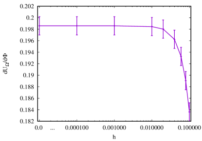
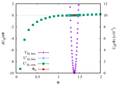
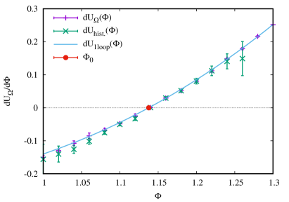
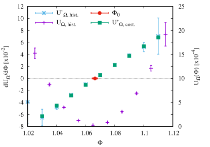
Figure 2: (left) Well defined continuum limit of $U_{\Omega,\rm{cnst.}}^{\prime}$ (2.5) with respect to step size $h\rightarrow 0$, it agrees with the continuum form $U_{\Omega,\rm{cont.}}^{\prime}$ (3.7) at $h=0$ for $h\leq 0.01$. (right) Effective potential and derivatives from histogram method and constrained simulations for the Abelian-Higgs model at $\beta=1.4,\kappa=0.17,\lambda=0.15$ on $\Omega=8^{4}$ lattices. The potential and its derivative diverge for $\Phi\rightarrow 0$.

In Fig. 2 (left) we investigate the continuum limit $h\rightarrow 0$ by plotting $U_{\Omega,\rm{cnst.}}^{\prime}$ for various simulation step sizes $h$, rapidly approaching the continuum value $U_{\Omega,\rm{cont.}}^{\prime}$ at $h=0$. We conclude that for the purpose of measuring the effective potential an integration step size of $h\leq 0.01$ is sufficient, for simplicity however, we use the continuum form anyhow.

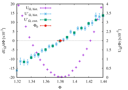
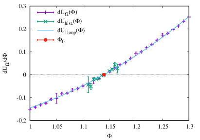
First results of the effective potential in the Higgs phase are presented in Fig. 2 (right) and Fig. 3 for $\beta=1.4,\kappa=0.17,\lambda=0.15$ and $\beta=0.6,\kappa=0.3,\lambda=1$ on $\Omega=8^{4}$ lattices, comparing the derivative of the constraint effective potential $U_{\Omega,\rm{cnst.}}^{\prime}$ with the effective potential $U_{\Omega,\rm{hist.}}$ and its derivative obtained from a standard histogram method, i.e., measuring the distribution of the field $\Phi=\sum_{n_{\mu}}\phi(n_{\mu})^{\dagger}\phi(n_{\mu})$ in an unconstrained simulation, appropriately binning it in a normalized histogram and taking the logarithm. The unconstrained simulation for the histogram method needs much more statistics than the individual constrained simulations combined to achieve comparable precision, only in the vicinity of the expectation value of the Higgs field $\Phi_{0}=\langle\Phi\rangle$. Note that the latter exactly coincides with the zero crossing of the derivative of the (constraint) effective potential, and we can read off the Higgs mass from the second derivative of the (constraint) effective potential at $\Phi_{0}$. Further notice in the right plot of Fig. 2 that with the new method to measure the derivative of the constraint effective potential, we can access the Higgs potential over the full parameter range of $\Phi$ with very high precision and find in the case of the Abelian-Higgs model that it diverges for $\Phi\rightarrow 0$, since only positive values of $\Phi$ are allowed by definition, see Eq. (3.3).

Figure 3: Effective potential and derivatives from histogram method and constrained simulations for the Abelian-Higgs model at $\beta=0.6,\kappa=0.3,\lambda=1$ (left) and $\beta=1.4,\kappa=0.17,\lambda=0.15$ (right, zoom of right plot in Fig. 2) on $\Omega=8^{4}$ lattices.

3.3 Comparison to the one-loop Higgs potential in unitary gauge

Note, we can write the action (3.2) in unitary gauge using the variable transformation proposed in [26] p.322, $\phi(n_{\mu})=\rho(n_{\mu})\exp{i\varphi(n_{\mu})}\;\Rightarrow\;\phi_{1}=\rho\cos\varphi,\;\phi_{2}=\rho\sin\varphi$:

$$S_{\rho}[V_{\mu},\rho] = \sum_{n_{\mu}}\bigg{[}\rho(n_{\mu})^{2}+\lambda(\rho(n_{\mu})^{2}-1)^{2}-2\kappa\rho(n_{\mu})\mbox{Re}\sum_{\mu}\rho(n_{\mu}+\hat{\mu})\overbrace{e^{-i\varphi(n_{\mu}+\hat{\mu})}U_{\mu}(n_{\mu})e^{i\varphi(n_{\mu})}}^{=V_{\mu}(n_{\mu})}\bigg{]},$$

with gauge invariant links $V_{\mu}(n_{\mu})$. This allows us to rewrite the constrained Hamiltonian as

$$\tilde{H}[V_{\mu},\rho]=S_{\rho}[V_{\mu},\rho]-\sum_{n_{\mu}}\ln[\rho(n_{\mu})]+\dfrac{1}{2}\sum_{n_{\mu}}\pi(n_{\mu})^{2}+\lambda^{(1)}\bigg{(}\dfrac{1}{\Omega}\sum_{n_{\mu}}\rho(n_{\mu})-\Phi\bigg{)},$$

where the $\ln(\rho)$ term enters from the Jacobian of the variable transformation and plays an important role: for small $\rho$ we get a diverging contribution to the action which pushes the system away from $\rho\leq 0$ which would be unphysical. The constrained equations of motion read

$$\dot{\rho}(n_{\mu})=\;\;\dfrac{\partial\tilde{H}}{\partial\pi(n_{\mu})}\,=\;\pi(n_{\mu})\;,\qquad\dot{\pi}(n_{\mu})=-\dfrac{\partial\tilde{H}}{\partial\rho(n_{\mu})}=-\dfrac{\partial S_{\rho}}{\partial\rho(n_{\mu})}+\dfrac{1}{\rho(n_{\mu})}-\dfrac{\lambda^{(1)}}{\Omega}$$

and derivatives of the constraint condition with respect to the molecular dynamics time allow us to solve for the Lagrange multiplier $\lambda^{(1)}$

$$\sum_{n_{\mu}}\dot{\rho}(n_{\mu})=\sum_{n_{\mu}}\pi(n_{\mu})=0\Rightarrow\sum_{n_{\mu}}\dot{\pi}(n_{\mu})=0\Rightarrow\lambda^{(1)}=\sum_{n_{\mu}}\bigg{(}\dfrac{1}{\rho(n_{\mu})}-\dfrac{\partial S_{\rho}}{\partial\rho(n_{\mu})}\bigg{)}.$$

We can use the standard leap-frog algorithm to perform the HMC updates as shown in [27] for a Higgs-Yukawa theory with $N_{f}$ fermions. In order to guarantee that the hidden constraint is fulfilled by the algorithm (note that the leap-frog algorithm would yield momenta fulfilling the constraint at the new time point, as it preserves linear constraints only in the momenta exactly), one has to initialize the (random) fictitious momenta $\pi(n_{\mu})$ in each trajectory accordingly, i.e., with respect to $\sum_{n_{\mu}}\pi(n_{\mu})=0$. During the constrained simulations we measure the derivative of the effective potential $U^{\prime}_{\Omega}(\Phi)=-\frac{1}{\Omega}\langle\lambda^{(1)}\rangle=\frac{1}{\Omega}\langle\sum_{n_{\mu}}[\partial S_{\rho}/\partial\rho(n_{\mu})-1/\rho(n_{\mu})]\rangle_{\Phi}$, where $\langle\ldots\rangle_{\Phi}$ means the expectation value at fixed $\Phi=\Omega^{-1}\sum_{n_{\mu}}\rho(n_{\mu})$.

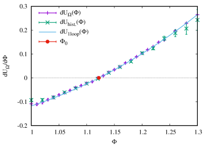
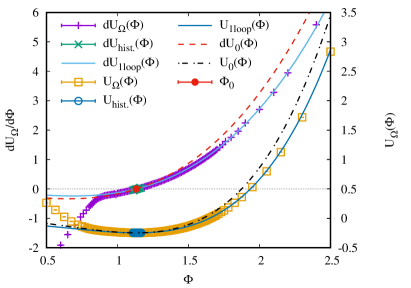
Results are presented in Fig. 4, where we compare the constraint effective potential with the effective potential measured by the histogram method in unconstrained simulations and with the finite, one-loop Higgs potential given by [23] (here $\tilde{\lambda}=4\lambda$)

$$V_{1}(\phi)=\frac{1}{2}m_{H}^{2}\phi^{2}+\left[\sqrt{\frac{\tilde{\lambda}}{2}}m_{H}-\frac{m_{H}}{16\pi^{2}\sqrt{2\tilde{\lambda}}}\Bigg{(}9\tilde{\lambda}^{2}+\frac{8\tilde{\lambda}^{2}m_{Z}^{4}}{m_{H}^{4}}\Bigg{)}\right]{\phi^{3}}+\frac{\phi^{4}}{4}\left[\tilde{\lambda}-\frac{1}{16\pi^{2}}\Bigg{(}\frac{32\tilde{\lambda}^{2}m_{Z}^{4}}{m_{H}^{4}}\Bigg{)}\right]$$ (3.8)

via fitting the (bare) Higgs mass $m_{H}$. We actually fit the derivative $U^{\prime}_{1\rm{loop}}(\Phi)=V^{\prime}_{1}(\Phi-\Phi_{0})$ to our measured $U^{\prime}_{\Omega}(\Phi)$, using the bare quartic coupling $\lambda$ and Z-boson mass given by the quasi-classical perturbative relation $m_{Z}=\sqrt{2\kappa g^{2}\langle\rho^{2}\rangle}$ [29], with the gauge coupling $g^{2}=1/\beta$. We choose a large value $\beta=8$ in order to stay in the weak coupling regime where we expect renormalization effects to be small. We find that the one-loop formula fits the constraint potential much better than the classical ansatz $U_{0}(\Phi)=-m_{H}^{2}\Phi^{2}/2+\lambda\Phi^{4}$, while the histogram data cannot differentiate the one-loop corrections within their limited range of $\Phi$.

$\qquad\quad\beta=8,\kappa=0.166,\lambda=0.15,\Omega=4^{4}\qquad\qquad\qquad\;\beta=8,\kappa=0.166,\lambda=0.15,\Omega=8^{4}\qquad\quad$
$\beta=8,\kappa=0.166,\lambda=0.15,\Omega=8^{3}\times 16$

Figure 4: Derivatives of the effective potential from histogram method and constrained simulations for the Abelian-Higgs model in unitary gauge at $\beta=8,\kappa=0.166$ and $\lambda=0.15$ and different lattice volumes $\Omega$, fitted with the derivative of the one-loop Higgs potential $V_{1}(\phi)$ [23] via $m_{H}$. The fits work quite well in the vicinity of $\Phi_{0}$, allowing us to extract reasonable Higgs masses, see also Table 1 and 2. The plot on the bottom to the right is an overview plot to the one on the left, showing the effects of the one-loop corrections compared to the classical potential $U_{0}(\Phi)=-m_{H}^{2}\Phi^{2}/2+\lambda\Phi^{4}$, where $m_{H}=2\Phi_{0}\sqrt{\lambda}$, also listed in Table 1. In order to plot the correct classical potential, the histogram, constraint and one-loop potentials are shifted by an integration constant $U_{0}(\Phi_{0})$ in the bottom right plot.

During the unconstrained simulations we also measure the two-point function [29]

$$C_{i}(\Delta t)=L_{t}^{-1}\sum_{t}\langle(O_{i}(t)-\langle O_{i}(t)\rangle)(O_{i}(t+\Delta t)-\langle O_{i}(t+\Delta t)\rangle)\rangle\approx\mathrm{cnst}(e^{-m\Delta t}+e^{-m(L_{t}-\Delta t)})$$ (3.9)

of the following lattice operators associated with quantum numbers $J^{PC}=0^{++}$ and $1^{--}$

$$O_{H}(t) = \Omega_{3}^{-1}\,\mathrm{Re}\sum_{x}\sum_{\mu=1,2,3}\rho(x,t)V_{\mu}(x,t)\rho(x+\hat{\mu},t)$$ (3.10)

$$O_{Z}(t) = \Omega_{3}^{-1}\,\mathrm{Im}\sum_{x}\sum_{\mu=1,2,3}\rho(x,t)V_{\mu}(x,t)\rho(x+\hat{\mu},t)$$ (3.11)

with the spatial (3D) volume $\Omega_{3}$. Fitting with the ansatz given on the right hand side of Eq. (3.9), discarding points with $\Delta t=0$ and $1$, we can extract the renormalized Higgs mass $m_{H,R}$ from the first operator $O_{H}$ and the gauge Z-boson (massive photon) mass $m_{Z,R}$ from $O_{Z}$ , the determined masses are summarized in Table 1. It can be seen, that renormalization effects are indeed small for $\beta=8$ (in contrast to $\beta=2.5$) and the masses agree quite well. We also list the classical values of the Higgs mass $2\Phi_{0}\sqrt{\lambda}$, derived from the classical ansatz $U_{0}(\Phi)$, which quantify the discrepancy of the classical Higgs potential ansatz, wich is just the tree level approximation, compared to the one-loop result.

$\beta$	$\lambda$	$\kappa$	$\Phi_{0}$	$\langle\rho^{2}\rangle$	$2\Phi_{0}\sqrt{\lambda}$	$m_{H}$	$m_{H,R}$	$m_{Z}$	$m_{Z,R}$
2.5	3.0	0.184	0.931(1)	0.913(2)	3.229(1)	4.071(1)	0.662(19)	0.362(1)	0.276(17)
8	0.15	0.164	1.100(1)	1.414(2)	0.852(1)	1.062(1)	1.054(19)	0.241(1)	0.176(13)
		0.166	1.133(1)	1.489(1)	0.878(1)	1.093(1)	1.099(21)	0.247(1)	0.185(12)
		0.168	1.164(1)	1.563(1)	0.902(1)	1.131(1)	1.162(23)	0.256(1)	0.209(14)
		0.17	1.194(1)	1.634(3)	0.925(1)	1.162(1)	1.218(28)	0.263(1)	0.224(17)
		0.2	1.555(1)	2.593(2)	1.204(1)	1.575(1)	1.787(26)	0.360(1)	0.328(19)

Table 1: Higgs and Z-boson masses from fits of the one-loop potential Eq. (3.8) to the constraint effective potential on $\Omega=8^{3}\times 16$ volumes via $m_{H}$ using the quasi-classical relation $m_{Z}=\sqrt{2\kappa g^{2}\langle\rho^{2}\rangle}$ [29], and from fits of the two-point function Eq. (3.9) using the operators given in Eq. (3.11) for $m_{H,R}$ and $m_{Z,R}$. We also list the classical values of the Higgs mass $2\Phi_{0}\sqrt{\lambda}$ quantifying the discrepancy of the classical potential compared to the one-loop result.

In Table 2 we show that the extracted Higgs mass does not depend on the volume and the precision of the new method does not deteriorate when increasing the latter, in contrast to the histogram method. We conclude that the constraint effective potential accurately determines the Higgs mass and reproduces not only the effective potential from the histogram method, but also compares very well to the one-loop Higgs potential given in Eq. (3.8) [23].

volume	$\Phi_{0}$	$m_{H}$	$U^{\prime}_{\Omega}(1.0)$	$U^{\prime}_{\Omega}(1.11)$	$U^{\prime}_{\mathrm{h.}}(1.11)$	$U^{\prime}_{\Omega}(1.15)$	$U^{\prime}_{\mathrm{h.}}(1.15)$	$U^{\prime}_{\Omega}(1.3)$
$4^{4}$	1.122(8)	1.068(1)	-0.099(3)	-0.016(3)	-0.014(3)	0.033(3)	0.034(3)	0.264(2)
$4^{3}\times 16$	1.132(1)	1.092(1)	-0.142(2)	-0.032(3)	-0.019(8)	0.018(3)	0.025(5)	0.261(3)
$8^{4}$	1.133(1)	1.093(1)	-0.159(2)	-0.040(2)	-0.043(17)	0.015(3)	0.017(9)	0.250(1)
$8^{3}\times 16$	1.133(1)	1.093(1)	-0.160(2)	-0.040(3)	-0.044(34)	0.013(3)	0.016(13)	0.252(1)

Table 2: Volume scaling of the Higgs mass $m_{H}$ from fits to the effective potential, except for the smallest volume we don’t see an effect, and comparison of the precision of the derivative of the potential obtained from constrained ($U_{\Omega}^{\prime}$) and unconstrained (histogram, $U_{\rm h.}^{\prime}$) simulations. Contrary to the latter, the error of results from constrained simulations does not increase with the volume. The results are for $\beta=8,\kappa=0.166$ and $\lambda=0.15$.

4 5D SU(2) GAUGE THEORY ON THE TORUS

The anisotropic Wilson plaquette action for a 5D SU(2) gauge theory with periodic (torus) boundary conditions is given by [30, 31, 32]

$$S_{W}^{tor}=\sum_{n_{\mu}}\sum_{n_{5}=0}^{N_{5}-1}\bigg{[}\frac{\beta_{4}}{2}\sum_{\mu<\nu}\mathrm{Re}\,\mbox{Tr}\{1-U_{\mu\nu}(n_{\mu},n_{5})\}+\frac{\beta_{5}}{2}\sum_{\mu}\mathrm{Re}\,\mbox{Tr}\{1-U_{\mu 5}(n_{\mu},n_{5})\}\bigg{]}\,,$$ (4.1)

where $\beta_{4}$ and $\beta_{5}$ are the gauge couplings associated with plaquettes spanning the standard four dimensions ($U_{\mu\nu}$) and the fifth dimension ($U_{\mu 5}$) respectively. The anisotropy is $\gamma=\sqrt{\beta_{5}/\beta_{4}}$ and in the classical limit $\gamma=a_{4}/a_{5}$, where $a_{4}$ denotes the lattice spacing in the usual four dimensions and $a_{5}$ denotes the lattice spacing in the extra dimension. The theory is defined on the periodic interval $I=\{n_{\mu},0\leq n_{5}<N_{5}\}$, where $(n_{\mu},n_{5})$, $\mu=0,1,2,3$ are the integer coordinates of the points of the five-dimensional lattice.

We start with a Higgs field $\mathcal{H}(n_{\mu})=\mbox{Tr}P_{5}(n_{\mu})$ given by the Polyakov loops in the extra dimension $P_{5}(n_{\mu})=\prod_{n_{5}=0}^{N_{5}-1}[U_{5}(n_{\mu},n_{5})]$, and the constraint condition is given by $\frac{1}{2\Omega}\sum_{n_{\mu}}\mbox{Tr}P_{5}(n_{\mu})=\Phi$ (4.2c). Hence, only the links in the extra dimension will be affected by the constraint, all other links $U_{\mu}(n_{\mu},n_{5})$, $\mu=0,1,2,3$ can be updated using the standard leapfrog method. For the links $U_{5}(n_{\mu},n_{5})$ and momenta $\pi_{5}(n_{\mu},n_{5})$ we apply the Rattle algorithm in appendix A.2 and find

$$\pi_{n+1/2} = \pi_{n}-\dfrac{h}{2}\biggr{(}\dfrac{\partial S}{\partial U_{n}}-\dfrac{\lambda_{n}^{(1)}}{8\Omega}\mbox{Tr}[...\sigma_{i}U_{n}...]\sigma^{i}\biggr{)}$$ (4.2a)

$$U_{n+1} = e^{h\pi_{n+1/2}}U_{n}$$ (4.2b)

$$0 = \dfrac{1}{2\Omega}\sum_{n_{\mu}}\mbox{Tr}P_{n+1}(n_{\mu})-\Phi=\dfrac{1}{2\Omega}\sum_{n_{\mu}}\mbox{Tr}\prod_{n_{5}=0}^{N_{5}-1}U_{n+1}-\Phi$$ (4.2c)

$$\pi_{n+1} = \pi_{n+1/2}-\dfrac{h}{2}\biggr{(}\dfrac{\partial S}{\partial U_{n+1}}-\dfrac{\lambda_{n}^{(2)}}{8\Omega}\mbox{Tr}[...\sigma_{i}U_{n+1}...]\sigma^{i}\biggr{)}$$ (4.2d)

$$0 = \dfrac{1}{8\Omega}\sum_{n_{\mu},n_{5}}\mbox{Tr}\{\mbox{Tr}[...\sigma_{i}U_{n+1}...]\sigma^{i}\pi_{n+1}\}$$ (4.2e)

The term $\mbox{Tr}[...\sigma_{i}U_{n}...]\sigma^{i}$ denotes a Polyakov line at $n_{\mu}$ with an insertion of $\sigma_{i}$ at $n_{5}$, summing over $i=1,2,3$ for the three Pauli matrices. The first three equations determine $(\pi_{n+1/2},U_{n+1},\lambda_{n}^{(1)})$, whereas the remaining two give $(\pi_{n+1},\lambda_{n}^{(2)})$.

We use a simple Secant method to get $\lambda_{n}^{(1)}$ up to machine precision, providing a precise root for the functional given by our constraint condition in Eq. (4.2c)

$$f(\lambda_{n}^{(1)}) = \dfrac{1}{2\Omega}\sum_{n_{\mu}}\mbox{Tr}P_{n+1}(n_{\mu},\lambda_{n}^{(1)})-\Phi=\dfrac{1}{2\Omega}\sum_{n_{\mu}}\mbox{Tr}\prod_{n_{5}=0}^{N_{5}-1}U_{n+1}(n_{\mu},n_{5},\lambda_{n}^{(1)})-\Phi$$

with $U_{n+1}(n_{\mu},n_{5},\lambda_{n}^{(1)})$ given in Eq. (4.2b). We iterate $\lambda^{(1)}_{n,k+1}=\lambda^{(1)}_{n,k}-f(\lambda^{(1)}_{n,k})[\lambda^{(1)}_{n,k}-\lambda^{(1)}_{n,k-1}]/[f(\lambda^{(1)}_{n,k})-f(\lambda^{(1)}_{n,k-1})]$, starting from an approximate solution $\lambda^{(1)}_{n,0}$ obtained by truncating the the exponential in (4.2b) after $\mathcal{O}(h^{2})$

$$\dfrac{\lambda^{(1)}_{n,0}}{8\Omega} = \bigg{\{}\sum_{n_{\mu},n_{5}}\bigg{(}\mbox{Tr}[...\dfrac{\partial S}{\partial U_{n}(n_{\mu},n_{5})}U_{n}(n_{\mu},n_{5})...]-\mbox{Tr}[...\pi_{n}^{2}(n_{\mu},n_{5})U_{n}(n_{\mu},n_{5})...]$$

$$-2\sum_{m_{5}>n_{5}}^{N_{5}-1}\mbox{Tr}[...\pi_{n}(n_{\mu},n_{5})U_{n}(n_{\mu},n_{5})...\pi_{n}(n_{\mu},m_{5})U_{n}(n_{\mu},m_{5})...]\bigg{)}\bigg{\}}/$$

$$\qquad\sum_{n_{\mu},n_{5}}\mbox{Tr}\{...\mbox{Tr}[...\sigma_{i}U_{n}(n_{\mu},n_{5})...]\sigma^{i}U_{n}(n_{\mu},n_{5})...\}$$

The iteration stops when $\lambda^{(1)}_{n,k+1}=\lambda^{(1)}_{n,k}$ or $f(\lambda^{(1)}_{n,k})=f(\lambda^{(1)}_{n,k-1})$ up to machine precision.

The second Lagrange multiplier is determined as (see appendix A.2 for details)

$$\dfrac{\lambda_{n}^{(2)}}{8\Omega} = \dfrac{\sum_{n_{\mu},n_{5}}\mbox{Tr}[...\sigma_{i}U_{n+1}(n_{\mu},n_{5})...]\mbox{Tr}[\sigma^{i}\partial S/\partial U_{n+1}(n_{\mu},n_{5})-2\sigma^{i}\pi_{n+1/2}(n_{\mu},n_{5})/h]}{\sum_{n_{\mu},n_{5}}\mbox{Tr}\{(\mbox{Tr}[...\sigma_{i}U_{n+1}(n_{\mu},n_{5})...]\sigma^{i})^{2}\}}$$ (4.4)

Again, we have to initialize the Polyakov lines to fulfill the constraint condition (4.2c), e.g., with the help of axial gauge, and when drawing the Gaussian-distributed random conjugate momenta $\pi^{r}(n_{\mu},n_{5})$ we have to ensure that they comply with the hidden constraint (4.2e), which we achieve via orthogonal projection

$$\pi_{0}(n_{\mu},n_{5})=\pi^{r}(n_{\mu},n_{5})-\dfrac{\sum_{n_{\mu},n_{5}}\mbox{Tr}\{\mbox{Tr}[...\sigma_{i}U(n_{\mu},n_{5})...]\sigma^{i}\pi^{r}(n_{\mu},n_{5})\}}{\sum_{n_{\mu},n_{5}}\mbox{Tr}\{(\mbox{Tr}[...\sigma_{i}U(n_{\mu},n_{5})...]\sigma^{i})^{2}\}}\mbox{Tr}[...\sigma_{i}U(n_{\mu},n_{5})...]\sigma^{i}$$

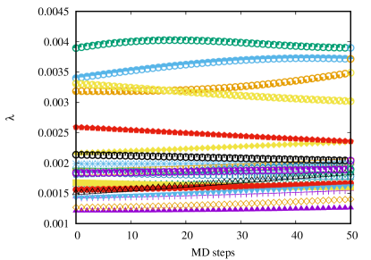
Fig. 5 shows that the Rattle algorithm for the 5D torus keeps the average Polyakov loop fixed (left plot). The Lagrange multiplier along a trajectory is plotted on the right.

\begin{overpic}[width=216.81pt]{figures/torattle2} \put(47.0,21.0){\scriptsize$\Phi=\dfrac{1}{2\Omega}\sum_{n_{\mu}}\mbox{Tr}P_{5}(n_{\mu})=0.4$} \end{overpic}

Figure 5: 5D Torus constrained HMC (Rattle) algorithm on a $2^{5}$ lattice: the individual Polyakov lines fluctuate around their average (left), guaranteed by an additional term in the Hamiltonian with the Lagrange multiplier $\lambda$ shown on the right evolving within different trajectories indicated by different colors/point styles.

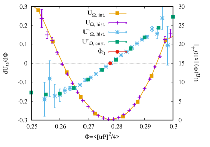
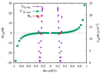
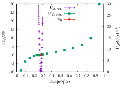
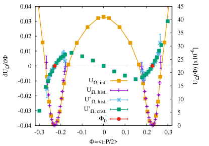
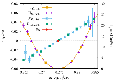
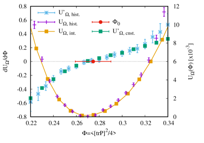
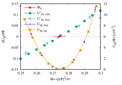
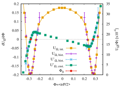
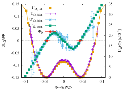
Figure 6: 5D Torus Effective Higgs Potential $U_{\Omega,\mathrm{hist.}}$ from the histogram method, its numerical derivative $U^{\prime}_{\Omega,\mathrm{hist.}}$, the derivative from constrained HMC $U^{\prime}_{\Omega,\mathrm{cnst.}}$ and its numerical integral $U_{\Omega,\mathrm{int.}}$ for $\beta_{4}=\beta_{5}=1.66,\Omega=8^{4},N_{5}=4$. The unconstrained expectation value of the Polyakov $\Phi_{0}=\langle\mbox{Tr}P_{5}/2\rangle=\pm 0.282$ has two degenerate minima (left column), while $\Phi_{0}=\langle(\mbox{Tr}P_{5})^{2}/4\rangle=0.278$ is always greater than zero of course (right column). The potentials (and derivatives) diverge at the boundaries because $-1\leq\mbox{Tr}P_{5}/2\leq 1$ and $0<(\mbox{Tr}P_{5})^{2}/4\leq 1$. The upper plots are a zoom of the plots in the second row.

Figure 7: 5D Torus Effective Higgs Potential $U_{\Omega,\mathrm{hist.}}$ from the histogram method, its numerical derivative $U^{\prime}_{\Omega,\mathrm{hist.}}$, the derivative from constrained HMC $U^{\prime}_{\Omega,\mathrm{cnst.}}$ and its numerical integral $U_{\Omega,\mathrm{int.}}$ for $\beta_{4}=1.0,\beta_{5}=2.8,\Omega=24\times 12^{3},N_{5}=4$ (upper plots). This point lies in the compcat phase of the theory, where dimensional reduction via compactification is expected. For $\mbox{Tr}P$ we find two degenerate minima, $(\mbox{Tr}P)^{2}$ only shows the positive potential minimum, of course. The lower plots are on smaller volumes for comparison, i.e. $V=4^{5}$ on the left and $8^{4}\times 4$ on the right. Note the different ranges for the abscissa and different scales for the ordinate.

Because of center symmetry, $\langle\mbox{Tr}P_{5}\rangle$ always vanishes in finite volume. Therefore, we further investigate the constraint $\frac{1}{4\Omega}\sum_{n_{\mu}}[\mbox{Tr}P_{5}({n_{\mu}})]^{2}=\Phi$ which fixes the Higgs field $\mathcal{H}=\frac{1}{8\Omega}\sum_{n_{\mu}}\mbox{Tr}[P_{5}({n_{\mu}})-P_{5}^{\dagger}({n_{\mu}})]^{2}=\Phi-1$ of the torus model and is invariant under center symmetry. The algorithm which fulfills the constraint is slightly more complicated than the one above and is formulated in appendix A.3. The implementation is equivalent to the previous cases and, therefore, we just summarize the important steps:

• initialize the field variables $q$ to fulfill the constraint $g(q)=0$

• draw (unconstrained) Gaussian distributed random momenta $p$

• project the momenta $p$ to satisfy the hidden constraint $\dot{g}(q,p)$

• propagate $p$ and $q$ as defined by the Rattle discretization

• accept new fields with probability $r=\text{min}[1,\exp(-\Delta H)]$

With the right tools at hand we now measure the constraint effective potentials $U_{\Omega}(\Phi)$ via their derivatives $U^{\prime}_{\Omega}(\Phi)=-\langle\lambda^{(1)}\rangle/\Omega$ for both cases $\langle\mbox{Tr}P_{5}/2\rangle$ and $\langle(\mbox{Tr}P_{5})^{2}/4\rangle$ of the 5D SU(2) gauge theory on the torus. In Fig. 6 we show effective Higgs potentials and their derivatives for the symmetric point $\beta_{4}=\beta_{5}=1.66$ on $\Omega=8^{4},N_{5}=4$ lattices. The results of the constrained method are in good agreement with the histogram potential in the vicinity of the expectation value of the Higgs field. The histogram method is limited to that narrow region, getting narrower the larger the lattice size, while the constraint effective potential can be measured very precisely over the whole parameter range. The unconstrained expectation values of the Higgs field $\Phi_{0}$ exactly coincide with the zero crossing of the (constraint) effective potentials. $\Phi_{0}=\langle\mbox{Tr}P_{5}/2\rangle=\pm 0.282$ is non-zero and we find two degenerate minima of the potential, the derivative of the constraint effective potential accordingly vanishes three times and its (numerical) integral shows the familiar Mexican hat form, which the histogram method cannot reproduce at all because of its limitations in potential width and accuracy. The upper plots in Fig. 7 present effective Higgs potentials for $\beta_{4}=1.0,\beta_{5}=2.8$ on $\Omega=24\times 12^{3},N_{5}=4$ lattices. This point lies in the so-called compact phase of the theory, where dimensional reduction via compactification is expected. Again we find two degenerate minima of the potential for $\Phi_{0}=\langle\mbox{Tr}P_{5}/2\rangle=\pm 0.228$ and the Mexican hat form is reproduced by the constraint effective potential only. The Higgs observable $(\mbox{Tr}P)^{2}$ only shows the positive potential minimum, and we also show results for two smaller volumes for comparison (lower plots). We conclude, that the constrained method is favorable to the histogram method in terms of accuracy and measurement range, the only drawback is the slower HMC algorithm which is essential for the first but not the latter.

5 5D SU(2) GAUGE THEORY ON THE ORBIFOLD

The orbifold theory we consider here is defined in the five-dimensional domain $I=\{n_{\mu},0\leq n_{5}\leq N_{5}\}$ with volume $N_{t}\times N_{s}^{3}\times N_{5}$. The anisotropic Wilson gauge action for an SU(2) gauge theory on this orbifold is given by [8]

$$S_{W}^{orb}=\sum_{n_{\mu}}\bigg{[}\frac{\beta_{4}}{2}\sum_{n_{5}=0}^{N_{5}}\sum_{\mu<\nu}w\,\mathrm{Re}\,\mbox{Tr}\{1-U_{\mu\nu}(n_{\mu},n_{5})\}+\frac{\beta_{5}}{2}\sum_{n_{5}=0}^{N_{5}-1}\sum_{\mu}\mathrm{Re}\,\mbox{Tr}\{1-U_{\mu 5}(n_{\mu},n_{5})\}\bigg{]}\,,$$ (5.1)

which follows the parametrization of Eq. (4.1). The weight $w$ is due to the orbifold geometry and takes a value $w=1/2$ for plaquettes $U_{\mu\nu}$ on the boundaries and it is $w=1$ elsewhere. The boundary links are in the gauge group U(1) and all other links are in SU(2). The anisotropy is $\gamma=\sqrt{\beta_{5}/\beta_{4}}$ and in the classical limit $\gamma=a_{4}/a_{5}$, where $a_{4}$ denotes the lattice spacing in the usual four dimensions and $a_{5}$ denotes the lattice spacing in the extra dimension. The theory is defined on the interval $I=\{n_{\mu},0\leq n_{5}\leq N_{5}\}$, where $(n_{\mu},n_{5})$, $\mu=0,1,2,3$ are the integer coordinates of the points. Given a constrained Hamiltonian for the Polyakov loop

$$P_{5}(n_{\mu}) = \prod_{n_{5}=0}^{N_{5}-1}[U_{5}(n_{\mu},n_{5})]\sigma_{3}\prod_{n_{5}=N_{5}-1}^{0}[U_{5}^{\dagger}(n_{\mu},n_{5})]\sigma_{3}$$ (5.2)

$$\tilde{H}[U_{5}] = S[U_{5}]+\sum_{n_{\mu}}\mbox{Tr}[\pi_{5}^{2}({\bf x})]+\lambda^{(1)}\bigg{(}\dfrac{1}{2\Omega}\sum_{n_{\mu}}\mbox{Tr}P_{5}(n_{\mu})-\Phi\bigg{)}$$ (5.3)

we solve the constrained equations of motion

$$\dot{U}_{5}(n_{\mu},n_{5}) = \pi_{5}(n_{\mu},n_{5})U_{5}(n_{\mu},n_{5}),$$

$$\dot{\pi}_{5}(n_{\mu},n_{5}) = -\dfrac{\partial S[U_{5}]}{\partial U_{5}(n_{\mu},n_{5})}+\dfrac{\lambda^{(1)}}{8\Omega}\mbox{Tr}[...\sigma_{i}U_{5}(n_{\mu},n_{5})...-...U_{5}^{\dagger}(n_{\mu},n_{5})\sigma_{i}...]\sigma^{i}$$

using the Rattle algorithm derived in appendix A.4. Like in the torus models, we use a Secant method to determine the first Lagrange multiplier $\lambda^{(1)}$, starting with an educated guess given by Eq. (A.4), and we have to initialize the momenta according to the hidden constraint.

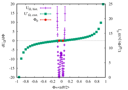
Figure 8: 5D Orbifold Effective Higgs Potential $U_{\Omega,\mathrm{hist.}}$ from the histogram method, its numerical derivative $U^{\prime}_{\Omega,\mathrm{hist.}}$ and the derivative from constrained HMC $U^{\prime}_{\Omega,\mathrm{cnst.}}=-\langle\lambda_{n}^{(1)}\rangle_{\Phi}/\Omega$ for the symmetric point $\beta_{4}=\beta_{5}=1.66,\Omega=8^{4},N_{5}=5$. This point lies in the Higgs phase, where the stick symmetry is broken and we find two degenerate minima of the potential. The left plot is a zoom of the right plot, where we show the full parameter range $-1<\mbox{Tr}P/2<1$.

The constraint effective potential is measured via its derivative $U^{\prime}_{\Omega,\mathrm{cnst.}}=-\langle\lambda_{n}^{(1)}\rangle_{\Phi}/\Omega$, a first result is shown in Fig. 8 for the symmetric point $\beta_{4}=\beta_{5}=1.66$ on a $\Omega=8^{4},N_{5}=4$ lattice. This point in parameter space lies in the Higgs phase close to the bulk-driven phase transition, see Fig. 1. The stick symmetry is broken and we find two degenerate minima of the potential. The constrained observable $\Phi$ however, is not yet the exact definition of the Higgs field in the orbifold model, which is given by $\mathcal{H}=\frac{1}{4\Omega}\sum_{n_{\mu}}\mbox{Tr}[P_{5}({n_{\mu}})-P_{5}^{\dagger}({n_{\mu}}),\sigma_{3}]^{2}$. The algorithm for the latter is in progress.

6 CONCLUSIONS AND OUTLOOK

We successfully implemented constrained hybrid Monte Carlo algorithms for the 4D Abelian-Higgs and a 5D SU(2) gauge theory with torus and orbifold boundary conditions which allow us to simulate systems with constraint conditions, which appear as Lagrange multiplier terms in the Hamiltonian. To our knowledge, this is the first time this problem has been solved for theories with gauge fields. In order to solve the constrained equations of motion we use an extension of the Newton-Störmer-Verlet-leapfrog method to general Hamiltonians for constrained systems, the so-called Rattle algorithm. This generalized leap-frog method has an additional half integration step for the conjugate momenta in order to evaluate the so-called hidden constraint, which is the derivative of the constraint condition with respect to molecular dynamics time and in our cases involves both fields and momenta, after a full integration time step, in order to calculate the Lagrange multipliers which ensure that the constraints are fulfilled. The algorithm fulfills all necessary geometrical properties, summarized in appendix A, and we numerically tested the time-reversibility and volume preservation. First simulation results show that the constraint effective potential accurately not only reproduces the effective potential from the histogram method, but drastically increases the range of accessibility of the effective potential, as the histogram method is restricted to the vicinity of the expectation value of the Higgs field, and the precision does not deteriorate when increasing the volume. Furthermore, for the 4D Abelian-Higgs model in unitary gauge we show that the constraint effective potential agrees well with the continuum one-loop Higgs potential given in Eq. (3.8) from [23]. We quantitatively compare the shape of the potentials for a weak gauge coupling. The Higgs mass determined from the potential agrees with the one extracted from fitting the two-point function of Higgs operators. The comparison to perturbative results is non-trivial for the other models due to the composite nature of the Higgs observables and, therefore, similar investigations are postponed to future work. In particular, we want to compare our constraint effective potentials in the 5D gauge theory cases with the one-loop effective Higgs potentials for the torus [33] and orbifold [11] models respectively.

We also plan to measure the constraint effective potentials on larger lattices and extract the Higgs masses in the different models considered. The latter is given by the second derivative of the constraint effective potential at the vacuum expectation value of the Higgs field and can be compared to the masses measured by different methods, e.g., by fitting two point functions from unconstrained simulations, which will allow us to study renormalization effects of the different mass determinations. Further we can compare the potentials measured in the different models and study the compactification and dimensional reduction scenarios of the 5D torus and orbifold models respectively via their connection to the 4D adjoint and Abelian-Higgs model.

Finally, an interesting application of these algorithms are effective Polyakov loop actions in finite temperature QCD. The effective Polyakov loop action (PLA) is the theory which results from integrating out all of the degrees of freedom of the theory, subject to the condition that the Polyakov lines are held fixed. This was studied in the strong coupling expansion [34], but also in full lattice QCD simulations. It was found that this effective theory is more tractable than the underlying lattice gauge theory (LGT) when confronting the sign problem at finite density, for recent advances see [35]. The developed algorithms in this article can be adapted to this problem, where the individual Polyakov lines and not their average over the whole lattice are constrained. This requires Lagrange multiplier terms for each Polyakov line, which appear as a product in the path integral or a sum in the Hamiltonian. There is no additional numerical effort though, instead of summing over the whole lattice to evaluate one Lagrange multiplier, one just calculates the individual factors locally. The extraction of the effective Polyakov loop potential can in principal proceed in a similar way as described in this work, or else by the relative weights approach as presented in [36].

7 ACKNOWLEDGMENTS

We thank Nikos Irges, Jean Zinn-Justin, Tomasz Korzec, Julius Kuti and Andreas Wipf for helpful discussions. We gratefully acknowledge the Gauss Center for Supercomputing (GCS) for providing computer time at the supercomputers JURECA/JUWELS at the Juelich Supercomputing Centre (JSC) under GCS/NIC project ID HWU24. This work was supported by the Deutsche Forschungsgemeinschaft in the SFB/TRR55 under Project B5 (R.H.).

Appendix A The Rattle algorithm for general constrained Hamiltonian systems

The most important numerical method for the solution of constrained Hamiltonian systems, the Rattle algorithm, is an adaptation of the Newton-Störmer-Verlet-leapfrog method that can be interpreted as a partitioned Runge-Kutta method and thus allows the extension to general Hamiltonians, c.f. [24, 25]. We consider mechanical systems with coordinates $q$ that are subject to constraints $g(q)=0$, and corresponding momenta $p$. The equations of motion are then given by

$$\dot{p} = -\nabla_{q}H(p,q)-\nabla_{q}g(q)\lambda$$

$$\dot{q} = \nabla_{p}H(p,q),\qquad 0=g(q),$$ (A.0.1)

where the Hamiltonian $H(p,q)$ is of the form

$$H(p,q)=\frac{1}{2}p^{T}M^{-1}p+U(q)$$ (A.0.2)

with a positive definite mass matrix $M$ and a potential $U(q)$. To compute the Lagrange multiplier $\lambda$, we differentiate the constraint $g(q(t))$ with respect to time, giving the so-called hidden constraint

$$0=\nabla_{q}g(q)^{T}\nabla_{p}H(p,q),$$ (A.0.3)

which is an invariant of the flow (A.0.1). We choose a step size h and discretized integration time $t_{n}=t_{0}+nh$. For initial values $(p_{n},q_{n})\in\mathcal{M}$, i.e., consistent with $g(q)=0$ and (A.0.3), the Rattle method yields an approximation $(p_{n+1},q_{n+1})$ which is again on the solution manifold $\mathcal{M}$:

$$p_{n+1/2} = p_{n}+\dfrac{h}{2}\bigg{(}\nabla_{q}U(q_{n})+\nabla_{q}g(q_{n})\lambda_{n}^{(1)}\bigg{)}$$ (A.0.4a)

$$q_{n+1} = q_{n}+hM^{-1}p_{n+1/2},$$ (A.0.4b)

$$0 = g(q_{n+1}),$$ (A.0.4c)

$$p_{n+1} = p_{n+1/2}+\frac{h}{2}\bigg{(}\nabla_{q}U(q_{n+1}),+\nabla_{q}g(q_{n+1})\lambda_{n}^{(2)}\bigg{)}$$ (A.0.4d)

$$0 = \nabla_{q}g(q_{n+1})^{T}M^{-1}p_{n+1}$$ (A.0.4e)

The first three equations determine $(p_{n+1/2},q_{n+1},\lambda_{n}^{(1)})$, whereas the remaining two give $(p_{n+1},\lambda_{n}^{(2)})$. Note that both Lagrangian multipliers are only intermediate variables and are not transported in the flow $\Phi_{h}$. We thus have a numerical flow $\Phi_{h}:\mathcal{M}\rightarrow\mathcal{M}$ with the following geometrical properties:

• the Rattle method is time-reversible, i.e., it holds $\rho\circ\Phi_{h}\circ\rho\circ\Phi_{h}=I$ with flipping the momenta denoted by $\rho(p,q)=(-p,q)$ ; if symmetry holds, i.e., $\Phi_{h}=\Phi_{-h}^{-1}$, this is equivalent to $\rho\circ\Phi_{h}=\Phi_{-h}\circ\rho$;

  • symmetry can be checked by exchanging the subscripts $n\leftrightarrow n+1$ and step size $h\leftrightarrow-h$, which has to leave the method unaltered. In our case, the first equation becomes the forth and vice-versa, if we change the denomination of both Lagrangian multipliers, which are only intermediate variables; the second equation remains unchanged; the nonlinear equations (A.0.4c),(A.0.4e) at time point $t_{n}+1$ are become those at $t_{n}$ (and vice-versa).

  • the condition $\rho\circ\Phi_{h}=\Phi_{-h}\circ\rho$ can be easily checked.

• ensures long-time energy conservation, to be verified via $\langle\exp(-\Delta H)=1\rangle$

• the Rattle algorithm is symplectic, i.e., the flow preserves areas in phase space

• det $\partial\Phi_{h}/\partial(p,q)=1$, i.e., the flow preserves the volume in phase space

• conservation of first integrals and preservation of adiabatic invariants

• provides a discrete virial theorem

For more details see [24, 25]. Now we summarize the algorithms for the various models.

A.1 Rattle algorithm for the 4D Abelian-Higgs model

Given a constraint condition for the complex variables $\phi(n_{\mu})$

$$\dfrac{1}{\Omega}\sum_{n_{\mu}}\phi^{\dagger}(n_{\mu})\phi(n_{\mu})=\Phi,$$ (A.1.1)

the constrained HMC (Rattle) algorithm can be formulated in the following way

$$\pi_{n+1/2} = \pi_{n}-\dfrac{h}{2}\bigg{(}\dfrac{\partial S}{\partial\phi_{n}}+\dfrac{2\phi_{n}\lambda_{n}^{(1)}}{\Omega}\bigg{)}$$ (A.1.2a)

$$\phi_{n+1} = \phi_{n}+h\pi_{n+1/2}$$ (A.1.2b)

$$0 = \dfrac{1}{\Omega}\sum_{n_{\mu}}\phi_{n+1}^{\dagger}\phi_{n+1}-\Phi$$ (A.1.2c)

$$\pi_{n+1} = \pi_{n+1/2}-\dfrac{h}{2}\bigg{(}\dfrac{\partial S}{\partial\phi_{n+1}}+\dfrac{2\phi_{n+1}\lambda_{n}^{(2)}}{\Omega}\bigg{)}$$ (A.1.2d)

$$0 = \dfrac{2}{\Omega}\sum_{n_{\mu}}\phi_{n+1}\pi_{n+1}$$ (A.1.2e)

Plugging $\pi_{n+1/2}$ into $\phi_{n+1}$ and evaluating the constraint gives $\lambda_{n}^{(1)}$:

$$0 = \sum\bigg{(}\dfrac{\phi_{n}}{h}+\pi_{n}-\dfrac{h}{2}\dfrac{\partial S}{\partial\phi_{n}}-\dfrac{h\phi_{n}\lambda_{n}^{(1)}}{\Omega}\bigg{)}^{2}-\dfrac{\Omega\Phi}{h^{2}}$$

$$= \cancel{\sum\dfrac{\phi_{n}^{2}}{h^{2}}}+\sum\pi_{n}^{2}+\sum\dfrac{h^{2}}{4}\bigg{(}\dfrac{\partial S}{\partial\phi_{n}}\bigg{)}^{2}+\dfrac{h^{2}\lambda_{n}^{(1)2}}{\Omega}\underbrace{\sum\dfrac{\phi_{n}^{2}}{\Omega}}_{=\Phi}+\dfrac{2}{h}\underbrace{\sum\phi_{n}\pi_{n}}_{=0}-\sum\phi_{n}\dfrac{\partial S}{\partial\phi_{n}}$$

$$-2\lambda_{n}^{(1)}\underbrace{\sum\dfrac{\phi_{n}^{2}}{\Omega}}_{=\Phi}-h\sum\pi_{n}\dfrac{\partial S}{\partial\phi_{n}}-\dfrac{2h\lambda_{n}^{(1)}}{\Omega}\underbrace{\sum\phi_{n}\pi_{n}}_{=0}+\dfrac{h^{2}\lambda_{n}^{(1)}}{\Omega}\sum\phi_{n}\dfrac{\partial S}{\partial\phi_{n}}-\cancel{\dfrac{\Omega\Phi}{h^{2}}}$$

$$= \lambda_{n}^{(1)2}+\lambda_{n}^{(1)}\bigg{(}\sum\dfrac{\phi_{n}}{\Phi}\dfrac{\partial S}{\partial\phi_{n}}-\dfrac{2\Omega}{h^{2}}\bigg{)}+\dfrac{\Omega}{\Phi}\sum\bigg{(}\dfrac{\pi_{n}^{2}}{h^{2}}-\dfrac{\phi_{n}}{h^{2}}\dfrac{\partial S}{\partial\phi_{n}}-\dfrac{\pi_{n}}{h}\dfrac{\partial S}{\partial\phi_{n}}+\dfrac{1}{4}\bigg{(}\dfrac{\partial S}{\partial\phi_{n}}\bigg{)}^{2}\bigg{)}$$

$$\Rightarrow\lambda_{n}^{(1)} = \dfrac{\Omega}{h^{2}}-\sum\dfrac{\phi_{n}}{2\Phi}\dfrac{\partial S}{\partial\phi_{n}}\pm\sqrt{\dfrac{\Omega^{2}}{h^{4}}+\bigg{(}\sum\dfrac{\phi_{n}}{2\Phi}\dfrac{\partial S}{\partial\phi_{n}}\bigg{)}^{2}-\dfrac{\Omega}{\Phi}\sum\bigg{(}\dfrac{\pi_{n}}{h}-\dfrac{1}{2}\dfrac{\partial S}{\partial\phi_{n}}\bigg{)}^{2}}$$

During numerical simulations it turns out that only the $-$ sign in front of the square root in $\lambda_{n}^{(1)}$ fulfills the constraint condition. Plugging $\pi_{n+1}$ into the hidden constraint (A.1.2e) gives

$$\lambda_{n}^{(2)} = \sum_{n_{\mu}}\bigg{(}\dfrac{\phi_{n+1}\pi_{n+1/2}}{h\Phi}-\dfrac{\phi_{n+1}}{2\Phi}\dfrac{\partial S}{\partial\phi_{n+1}}\bigg{)}$$

When drawing the Gaussian-distributed random conjugate momenta $\pi^{r}(n_{\mu})$ we have to ensure that they comply with the hidden constraint, which we achieve via orthogonal projection

$$\pi_{0}(n_{\mu})=\pi^{r}(n_{\mu})-\dfrac{\phi(n_{\mu})}{\Omega\Phi}\sum_{m_{\mu}}\pi^{r}(m_{\mu})\phi(m_{\mu}),$$

as can be verified by plugging it back into (A.1.2e).

A.2 Rattle algorithm for 5D SU(2) gauge theory on the torus fixing $\langle\mbox{Tr}P\rangle$

Given a constraint condition for the SU(2) link variables $U_{5}(n_{\mu})$ in the fifth dimension

$$\dfrac{1}{2\Omega}\sum_{n_{\mu}}\mbox{Tr}\prod_{n_{5}=0}^{N_{5}-1}U_{5}(n_{\mu},n_{5})=\Phi$$ (A.2.1)

the constrained HMC (Rattle) algorithm can be formulated in the following way

$$\pi_{n+1/2} = \pi_{n}-\dfrac{h}{2}\bigg{(}\dfrac{\partial S}{\partial U_{n}}-\dfrac{\lambda_{n}^{(1)}}{8\Omega}\mbox{Tr}[...\sigma_{i}U_{n}...]\sigma^{i}\bigg{)}$$ (A.2.2a)

$$U_{n+1} = e^{h\pi_{n+1/2}}U_{n}$$ (A.2.2b)

$$0 = \dfrac{1}{2\Omega}\sum_{n_{\mu}}\mbox{Tr}\prod_{n_{5}=0}^{N_{5}-1}U_{n+1}(n_{\mu},n_{5})-\Phi$$ (A.2.2c)

$$\pi_{n+1} = \pi_{n+1/2}-\dfrac{h}{2}\bigg{(}\dfrac{\partial S}{\partial U_{n+1}}-\dfrac{\lambda_{n}^{(2)}}{8\Omega}\mbox{Tr}[...\sigma_{i}U_{n+1}...]\sigma^{i}\bigg{)}$$ (A.2.2d)

$$0 = \sum_{n_{\mu},n_{5}}\mbox{Tr}\{\mbox{Tr}[...\sigma_{i}U_{n+1}(n_{\mu},n_{5})...]\sigma^{i}\pi_{n+1}(n_{\mu},n_{5})\}$$ (A.2.2e)

where $\mbox{Tr}[...\sigma_{i}U_{5}(n_{\mu},n_{5})...]\sigma^{i}$ is the derivative of the constraint with respect to $U_{5}(n_{\mu},n_{5})$, using

$$\partial_{5}\mbox{Tr}U_{5} \equiv \dfrac{i}{2}\sigma^{a}\partial_{5,a}\mbox{Tr}U_{5}=\dfrac{i}{2}\sigma^{a}\lim_{\epsilon\rightarrow 0}\dfrac{\mbox{Tr}(e^{i\epsilon\frac{\sigma_{a}}{2}}U_{5})-\mbox{Tr}U_{5}}{\epsilon}=-\dfrac{1}{4}\mbox{Tr}(\sigma_{a}U_{5})\sigma^{a}$$

When evaluating the constraint condition for $U_{n+1}$ we truncate the exponential in (A.2.2b)

$$e^{h\pi_{n+1/2}} = 1+h\pi_{n}-\dfrac{h^{2}}{2}\dfrac{\partial S}{\partial U_{n}}+\dfrac{\lambda_{n}^{(1)}h^{2}}{16\Omega}\mbox{Tr}[...\sigma_{i}U_{n}...]\sigma^{i}+\dfrac{h^{2}}{2}\pi_{n}^{2}+\mathcal{O}(h^{3})$$ (A.2.3)

and solve for $\lambda_{n}^{(1)}$ up to the same order

$$\Phi = \dfrac{1}{2\Omega}\sum_{n_{\mu}}\mbox{Tr}[e^{h\pi_{n+1/2}(n_{\mu},0)}U_{n}(n_{\mu},0)\ldots e^{h\pi_{n+1/2}(n_{\mu},N_{5}-1)}U_{n}(n_{\mu},N_{5}-1)]$$

Φ $$= \dfrac{1}{2\Omega}\sum_{n_{\mu}}\bigg{\{}h\sum_{n_{5}=0}^{N_{5}-1}\bigg{(}\underbrace{\mbox{Tr}[...\pi_{n}(n_{\mu},n_{5})U_{n}(n_{\mu},n_{5})...]}_{\sum\ldots=0}-\dfrac{h}{2}\mbox{Tr}[...\dfrac{\partial S}{\partial U_{n}(n_{\mu},n_{5})}U_{n}(n_{\mu},n_{5})...]$$

$$+\dfrac{\lambda_{n}^{(1)}h}{16\Omega}\mbox{Tr}\{...\mbox{Tr}[...\sigma_{i}U_{n}(n_{\mu},n_{5})...]\sigma^{i}U_{n}(n_{\mu},n_{5})...\}+\dfrac{h}{2}\mbox{Tr}[...\pi_{n}^{2}(n_{\mu},n_{5})U_{n}(n_{\mu},n_{5})...]$$

$$+h\sum_{m_{5}>n_{5}}^{N_{5}-1}\mbox{Tr}[...\pi_{n}(n_{\mu},n_{5})U_{n}(n_{\mu},n_{5})...\pi_{n}(n_{\mu},m_{5})U_{n}(n_{\mu},m_{5})...]\bigg{)}+\cancel{\mbox{Tr}P_{n}(n_{\mu})}\bigg{\}}+\mathcal{O}(h^{3})$$

$$\dfrac{\lambda_{n}^{(1)}}{8\Omega} = \bigg{\{}\sum_{n_{\mu},n_{5}}\bigg{(}\mbox{Tr}[...\dfrac{\partial S}{\partial U_{n}(n_{\mu},n_{5})}U_{n}(n_{\mu},n_{5})...]-\mbox{Tr}[...\pi_{n}^{2}(n_{\mu},n_{5})U_{n}(n_{\mu},n_{5})...]$$

$$-2\sum_{m_{5}>n_{5}}^{N_{5}-1}\mbox{Tr}[...\pi_{n}(n_{\mu},n_{5})U_{n}(n_{\mu},n_{5})...\pi_{n}(n_{\mu},m_{5})U_{n}(n_{\mu},m_{5})...]\bigg{)}\bigg{\}}/$$

$$\qquad\sum_{n_{\mu},n_{5}}\mbox{Tr}\{...\mbox{Tr}[...\sigma_{i}U_{n}(n_{\mu},n_{5})...]\sigma^{i}U_{n}(n_{\mu},n_{5})...\}+\mathcal{O}(h^{3})$$

We use a Secant method to get the Lagrange multiplier with machine precision. Plugging $\pi_{n+1}$ (A.2.2d) into the hidden constraint (A.2.2e) gives $\lambda_{n}^{(2)}$:

$$\dfrac{\lambda_{n}^{(2)}}{8\Omega} = \sum_{n_{\mu},n_{5}}\bigg{(}\mbox{Tr}[...\sigma_{i}U_{n+1}(n_{\mu},n_{5})...]\sigma^{i}\partial S/\partial U_{n+1}(n_{\mu},n_{5})$$

$$\quad-2\mbox{Tr}[...\sigma_{i}U_{n+1}(n_{\mu},n_{5})...]\sigma^{i}\pi_{n+1/2}(n_{\mu},n_{5})/h\bigg{)}/$$

$$\qquad\sum_{n_{\mu},n_{5}}\mbox{Tr}\{(\mbox{Tr}[...\sigma_{i}U_{n+1}(n_{\mu},n_{5})...]\sigma^{i})^{2}\}$$

Again, when drawing the Gaussian-distributed random conjugate momenta $\pi^{r}(n_{\mu},n_{5})$ we have to ensure that they comply with the hidden constraint, which we achieve by orthogonal projection

$$\pi_{0}(n_{\mu},n_{5}) = \pi^{r}(n_{\mu},n_{5})-\mu\mbox{Tr}[...\sigma_{i}U(n_{\mu},n_{5})...]\sigma^{i}$$

and solving for $\mu$ by plugging $\pi_{0}(n_{\mu},n_{5})$ into the hidden constraint (A.2.2e)

$$\mu = \dfrac{\sum_{n_{\mu},n_{5}}\mbox{Tr}\{\mbox{Tr}[...\sigma_{i}U(n_{\mu},n_{5})...]\sigma^{i}\pi^{r}(n_{\mu},n_{5})\}}{\sum_{n_{\mu},n_{5}}\mbox{Tr}\{(\mbox{Tr}[...\sigma_{i}U(n_{\mu},n_{5})...]\sigma^{i})^{2}\}}$$

A.3 Rattle algorithm for 5D SU(2) gauge theory on the torus fixing $\langle(\mbox{Tr}P_{5})^{2}\rangle$

Given a constraint condition for the average of the squared trace of the Polyakov loop $P_{5}$ in the extra dimension constructed from SU(2) link variables $U_{5}(n_{\mu})$

$$\dfrac{1}{4\Omega}\sum_{n_{\mu}}(\mbox{Tr}P_{n+1})^{2}=\dfrac{1}{4\Omega}\sum_{n_{\mu}}\mbox{Tr}\prod_{n_{5}=0}^{N_{5}-1}U_{n+1}(n_{\mu},n_{5})\mbox{Tr}\prod_{n_{5}=0}^{N_{5}-1}U_{n+1}(n_{\mu},n_{5})=\Phi$$ (A.3.1)

the constrained HMC (Rattle) algorithm can be formulated in the following way

$$\pi_{n+1/2} = \pi_{n}-\dfrac{h}{2}\bigg{(}\dfrac{\partial S}{\partial U_{n}}-\dfrac{\lambda_{n}^{(1)}}{16\Omega}\mbox{Tr}P_{n}\mbox{Tr}[...\sigma_{i}U_{n}...]\sigma^{i}\bigg{)}$$ (A.3.2a)

$$U_{n+1} = e^{h\pi_{n+1/2}}U_{n}$$ (A.3.2b)

$$0 = \dfrac{1}{4\Omega}\sum_{n_{\mu}}\mbox{Tr}\prod_{n_{5}=0}^{N_{5}-1}U_{n+1}(n_{\mu},n_{5})\mbox{Tr}\prod_{n_{5}=0}^{N_{5}-1}U_{n+1}(n_{\mu},n_{5})-\Phi$$ (A.3.2c)

$$\pi_{n+1} = \pi_{n+1/2}-\dfrac{h}{2}\bigg{(}\dfrac{\partial S}{\partial U_{n+1}}-\dfrac{\lambda_{n}^{(2)}}{16\Omega}\mbox{Tr}P_{n+1}\mbox{Tr}[...\sigma_{i}U_{n+1}...]\sigma^{i}\bigg{)}$$ (A.3.2d)

$$0 = \sum_{n_{\mu},n_{5}}\mbox{Tr}P_{n+1}\mbox{Tr}\{\mbox{Tr}[...\sigma_{i}U_{n+1}(n_{\mu},n_{5})...]\sigma^{i}\pi_{n+1}(n_{\mu},n_{5})\}$$ (A.3.2e)

with $2\mbox{Tr}P_{5}(n_{\mu})\mbox{Tr}[...\sigma_{i}U_{5}(n_{\mu},n_{5})...]\sigma^{i}$ the derivative of the constraint with respect to $U_{5}(n_{\mu},n_{5})$. Again, we truncate the exponential in (A.3.2b)

$$e^{h\pi_{n+1/2}} = 1+h\pi_{n}-\dfrac{h^{2}}{2}\dfrac{\partial S}{\partial U_{n}}+\dfrac{\lambda_{n}^{(1)}h^{2}}{32\Omega}\mbox{Tr}P_{n}\mbox{Tr}[...\sigma_{i}U_{n}...]\sigma^{i}+\dfrac{h^{2}}{2}\pi_{n}^{2}+\mathcal{O}(h^{3})$$ (A.3.3)

and plug $U_{n+1}$ into the constraint condition, solving for $\lambda_{n}^{(1)}$ up to the same order

$$\Phi = \dfrac{1}{4\Omega}\sum_{n_{\mu}}\bigg{(}\mbox{Tr}[e^{h\pi_{n+1/2}(n_{\mu},0)}U_{n}(n_{\mu},0)\ldots e^{h\pi_{n+1/2}(n_{\mu},N_{5}-1)}U_{n}(n_{\mu},N_{5}-1)]\bigg{)}^{2}$$

Φ $$= \dfrac{1}{4\Omega}\sum_{n_{\mu}}\bigg{\{}\cancel{(\mbox{Tr}P_{n})^{2}}+2h\sum_{n_{5}=0}^{N_{5}-1}\bigg{(}\underbrace{\mbox{Tr}[...\pi_{n}U_{n}...]}_{\sum\ldots=0}-\dfrac{h}{2}\mbox{Tr}[...\dfrac{\partial S}{\partial U_{n}(n_{\mu},n_{5})}U_{n}(n_{\mu},n_{5})...]$$

$$+\dfrac{\lambda_{n}^{(1)}h}{32}\mbox{Tr}P_{n}\mbox{Tr}\{...\mbox{Tr}[...\sigma_{i}U_{n}(n_{\mu},n_{5})...]\sigma^{i}U_{n}(n_{\mu},n_{5})...\}+\dfrac{h}{2}\mbox{Tr}[...\pi_{n}^{2}(n_{\mu},n_{5})U_{n}(n_{\mu},n_{5})...]$$

$$+h\sum_{m_{5}>n_{5}}^{N_{5}-1}\mbox{Tr}[...\pi_{n}(n_{\mu},n_{5})U_{n}(n_{\mu},n_{5})...\pi_{n}(n_{\mu},m_{5})U_{n}(n_{\mu},m_{5})...]\bigg{)}\,\mbox{Tr}P_{n}(n_{\mu})$$

$$+h^{2}\sum_{n_{5}=0}^{N_{5}-1}\sum_{m_{5}=0}^{N_{5}-1}\mbox{Tr}[...\pi_{n}(n_{\mu},n_{5})U_{n}(n_{\mu},n_{5})...]\mbox{Tr}[...\pi_{n}(n_{\mu},m_{5})U_{n}(n_{\mu},m_{5})...]\bigg{\}}+\mathcal{O}(h^{3})$$

$$\dfrac{\lambda_{n}^{(1)}}{16\Omega} = \bigg{\{}\sum_{n_{\mu}}\bigg{[}\mbox{Tr}P_{n}(n_{\mu})\sum_{n_{5}}\bigg{(}\mbox{Tr}[...\dfrac{\partial S}{\partial U_{n}(n_{\mu},n_{5})}U_{n}(n_{\mu},n_{5})...]-\mbox{Tr}[...\pi_{n}^{2}(n_{\mu},n_{5})U_{n}(n_{\mu},n_{5})...]$$

$$-2\sum_{m_{5}>n_{5}}^{N_{5}-1}\mbox{Tr}[...\pi_{n}(n_{\mu},n_{5})U_{n}(n_{\mu},n_{5})...\pi_{n}(n_{\mu},m_{5})U_{n}(n_{\mu},m_{5})...]\bigg{)}$$

$$-\sum_{n_{5}}\sum_{m_{5}}\mbox{Tr}[...\pi_{n}(n_{\mu},n_{5})U_{n}(n_{\mu},n_{5})...]\mbox{Tr}[...\pi_{n}(n_{\mu},m_{5})U_{n}(n_{\mu},m_{5})...]\bigg{]}\bigg{\}}$$

$$\qquad/\sum_{n_{\mu},n_{5}}(\mbox{Tr}P_{n}(n_{\mu}))^{2}\mbox{Tr}\{...\mbox{Tr}[...\sigma_{i}U_{n}(n_{\mu},n_{5})...]\sigma^{i}U_{n}(n_{\mu},n_{5})...\}+\mathcal{O}(h^{3})$$

We use a Secant method to get the Lagrange multiplier with machine precision. Plugging $\pi_{n+1}$ (A.3.2d) into the hidden constraint (A.3.2e) gives $\lambda_{n}^{(2)}$:

$$\dfrac{\lambda_{n}^{(2)}}{16\Omega} = \sum_{n_{\mu},n_{5}}\bigg{(}\mbox{Tr}P_{n}(n_{\mu})\mbox{Tr}[...\sigma_{i}U_{n+1}(n_{\mu},n_{5})...]\sigma^{i}\partial S/\partial U_{n+1}(n_{\mu},n_{5})$$

$$\qquad-2\mbox{Tr}P_{n}(n_{\mu})\mbox{Tr}[...\sigma_{i}U_{n+1}(n_{\mu},n_{5})...]\sigma^{i}\pi_{n+1/2}(n_{\mu},n_{5})/h\bigg{)}/$$

$$\qquad\sum_{n_{\mu},n_{5}}(\mbox{Tr}P_{n}(n_{\mu}))^{2}\mbox{Tr}\{(\mbox{Tr}[...\sigma_{i}U_{n+1}(n_{\mu},n_{5})...]\sigma^{i})^{2}\}$$

Again, when drawing the Gaussian-distributed random conjugate momenta $\pi^{r}(n_{\mu},n_{5})$ we have to ensure that they comply with the hidden constraint, which we achieve by the orthogonal projection

$$\pi_{0}(n_{\mu},n_{5}) = \pi^{r}(n_{\mu},n_{5})-\mu\mbox{Tr}P\mbox{Tr}[...\sigma_{i}U(n_{\mu},n_{5})...]\sigma^{i}$$

and solving for $\mu$ by plugging $\pi_{0}(n_{\mu},n_{5})$ into the hidden constraint (A.3.2e)

$$\mu = \dfrac{\sum_{n_{\mu},n_{5}}\mbox{Tr}\{\mbox{Tr}P\mbox{Tr}[...\sigma_{i}U(n_{\mu},n_{5})...]\sigma^{i}\pi^{r}(n_{\mu},n_{5})\}}{\sum_{n_{\mu},n_{5}}\mbox{Tr}\{(\mbox{Tr}P\mbox{Tr}[...\sigma_{i}U(n_{\mu},n_{5})...]\sigma^{i})^{2}\}}$$

A.4 Rattle algorithm for the 5D orbifold gauge-Higgs model fixing $\langle\mbox{Tr}P\rangle$

Given a constraint condition for the SU(2) link variables $U_{5}(n_{\mu})$ in the fifth dimension

$$\dfrac{1}{2\Omega}\sum_{n_{\mu},n_{5}}\prod_{n_{5}=0}^{N_{5}-1}[U_{5}(n_{\mu},n_{5})]\sigma_{3}\prod_{n_{5}=N_{5}-1}^{0}[U_{5}^{\dagger}(n_{\mu},n_{5})]\sigma_{3}=\Phi,$$ (A.4.1)

the constrained HMC (Rattle) algorithm can be formulated in the following way

$$\pi_{n+1/2} = \pi_{n}-\dfrac{h}{2}\bigg{(}\dfrac{\partial S}{\partial U_{n}}-\dfrac{\lambda_{n}^{(1)}}{8\Omega}\mbox{Tr}[...\sigma_{i}U_{n}...-...U_{n}^{\dagger}\sigma_{i}...]\sigma^{i}\bigg{)}$$ (A.4.2a)

$$U_{n+1} = e^{h\pi_{n+1/2}}U_{n},\qquad U_{n+1}^{\dagger}=U_{n}^{\dagger}e^{-h\pi_{n+1/2}}$$ (A.4.2b)

$$0 = \dfrac{1}{2\Omega}\sum_{n_{\mu}}\mbox{Tr}\prod_{n_{5}=0}^{N_{5}-1}[U_{n+1}(n_{\mu},n_{5})]\sigma_{3}\prod_{n_{5}=N_{5}-1}^{0}[U_{n+1}^{\dagger}(n_{\mu},n_{5})]\sigma_{3}-\Phi$$ (A.4.2c)

$$\pi_{n+1} = \pi_{n+1/2}-\dfrac{h}{2}\bigg{(}\dfrac{\partial S}{\partial U_{n+1}}-\dfrac{\lambda_{n}^{(2)}}{8\Omega}\mbox{Tr}[...\sigma_{i}U_{n+1}...-...U_{n+1}^{\dagger}\sigma_{i}...]\sigma^{i}\bigg{)}$$ (A.4.2d)

$$0 = \dfrac{1}{8\Omega}\sum_{n_{\mu},n_{5}}\mbox{Tr}\{\mbox{Tr}[...\sigma_{i}U_{n+1}(n_{\mu},n_{5})...-...U_{n+1}^{\dagger}(n_{\mu},n_{5})\sigma_{i}...]\sigma^{i}\pi_{n+1}(n_{\mu},n_{5})\}\qquad$$ (A.4.2e)

The first three lines determine $(\pi_{n+1/2},U_{n+1},\lambda_{n}^{(1)})$, whereas the remaining two give $(\pi_{n+1},\lambda_{n}^{(2)})$. Again, we truncate the exponentials in (A.4.2b)

$$e^{h\pi_{n+1/2}} = 1+h\pi_{n}-\dfrac{h^{2}}{2}\dfrac{\partial S}{\partial U_{n}}+\dfrac{h^{2}\lambda}{16\Omega}\mbox{Tr}[...\sigma_{i}U_{n}...-...U_{n}^{\dagger}\sigma_{i}...]\sigma^{i}+\dfrac{h^{2}}{2}\pi_{n}^{2}+\mathcal{O}(h^{3})$$

$$e^{-h\pi_{n+1/2}} = 1-h\pi_{n}+\dfrac{h^{2}}{2}\dfrac{\partial S}{\partial U_{n}}-\dfrac{h^{2}\lambda}{16\Omega}\mbox{Tr}[...\sigma_{i}U_{n}...-...U_{n}^{\dagger}\sigma_{i}...]\sigma^{i}+\dfrac{h^{2}}{2}\pi_{n}^{2}+\mathcal{O}(h^{3})$$

and solve the constraint (A.4.2c) for the first Lagrange multipliers

$$\dfrac{\lambda_{n}^{(1)}}{8\Omega} = \bigg{\{}\sum_{n_{\mu},n_{5}}\bigg{(}\mbox{Tr}[...\dfrac{\partial S}{\partial U_{n}(n_{\mu},n_{5})}U_{n}(n_{\mu},n_{5})...-...U_{n}^{\dagger}(n_{\mu},n_{5})\dfrac{\partial S}{\partial U_{n}(n_{\mu},n_{5})}...]$$

$$\qquad-\mbox{Tr}[...\pi_{n}^{2}(n_{\mu},n_{5})U_{n}(n_{\mu},n_{5})...+...U_{n}^{\dagger}(n_{\mu},n_{5})\pi_{n}^{2}(n_{\mu},n_{5})...]$$

$$\qquad-2\sum_{m_{5}}\mbox{Tr}\bigg{[}...\pi_{n}(n_{\mu},n_{5})U_{n}(n_{\mu},n_{5})...\pi_{n}(n_{\mu},m_{5}>n_{5})U_{n}(n_{\mu},m_{5}>n_{5})...$$

$$\qquad\qquad\qquad-...\pi_{n}(n_{\mu},n_{5})U_{n}(n_{\mu},n_{5})...U_{n}^{\dagger}(n_{\mu},m_{5})\pi_{n}(n_{\mu},m_{5})...$$

$$\qquad\qquad\qquad+...U_{n}^{\dagger}(n_{\mu},m_{5}>n_{5})\pi_{n}(n_{\mu},m_{5}>n_{5})...U_{n}^{\dagger}(n_{\mu},n_{5})\pi_{n}(n_{\mu},n_{5})...\bigg{]}\bigg{)}\bigg{\}}/$$

$$\sum_{n_{\mu},n_{5}}\mbox{Tr}[...\sigma_{i}U_{n}(n_{\mu},n_{5})...-...U_{n}^{\dagger}(n_{\mu},n_{5})\sigma_{i}...]\mbox{Tr}[...\sigma^{i}U_{n}(n_{\mu},n_{5})...-...U_{n}^{\dagger}(n_{\mu},n_{5})\sigma^{i}...]$$

$$+\mathcal{O}(h^{3})$$

We use a Secant method to get the Lagrange multiplier with machine precision. Plugging $\pi_{n+1}$ (A.4.2d) into the hidden constraint (A.4.2e) gives $\lambda_{n}^{(2)}$:

$$\dfrac{\lambda_{n}^{(2)}}{8\Omega} = \sum_{n_{\mu},n_{5}}\bigg{(}\mbox{Tr}\{\mbox{Tr}[...\sigma_{i}U_{n}...-...U_{n}^{\dagger}\sigma_{i}...]\sigma^{i}\partial S/\partial U_{n+1}(n_{\mu},n_{5})\}$$

$$\qquad\quad-2\mbox{Tr}\{\mbox{Tr}[...\sigma_{i}U_{n}...-...U_{n}^{\dagger}\sigma_{i}...]\sigma^{i}\pi_{n+1/2}(n_{\mu},n_{5})\}/h\bigg{)}/$$

$$\quad\sum_{n_{\mu},n_{5}}\mbox{Tr}\{(\mbox{Tr}[...\sigma_{i}U_{n+1}...-...U_{n+1}^{\dagger}\sigma_{i}...]\sigma^{i})^{2}\}$$

We initialize momenta $\pi_{0}$ from Gaussian-random distributed $\pi^{r}$ via orthogonal projection

$$\pi_{0}(n_{\mu},n_{5}) = \pi^{r}(n_{\mu},n_{5})-\mu\mbox{Tr}[...\sigma_{i}U(n_{\mu},n_{5})...-...U(n_{\mu},n_{5})^{\dagger}\sigma_{i}...]\sigma^{i}$$

$$0 = \dfrac{1}{8\Omega}\sum_{n_{\mu},n_{5}}\mbox{Tr}\{\mbox{Tr}[...\sigma_{i}U(n_{\mu},n_{5})...-...U^{\dagger}(n_{\mu},n_{5})\sigma_{i}...]\sigma^{i}\pi_{0}(n_{\mu},n_{5})\}$$

$$\Rightarrow\mu = \dfrac{\sum_{n_{\mu},n_{5}}\mbox{Tr}\{\mbox{Tr}[...\sigma_{i}U(n_{\mu},n_{5})...-...U(n_{\mu},n_{5})^{\dagger}\sigma_{i}...]\sigma^{i}\pi^{r}(n_{\mu},n_{5})\}}{\sum_{n_{\mu},n_{5}}\mbox{Tr}\{(\mbox{Tr}[...\sigma_{i}U(n_{\mu},n_{5})...-...U(n_{\mu},n_{5})^{\dagger}\sigma_{i}...]\sigma^{i})^{2}\}}$$

Appendix B References