Surrogate Optimization of Deep Neural Networks for Groundwater Predictions

Abstract

Sustainable management of groundwater resources under changing climatic conditions require an application of reliable and accurate predictions of groundwater levels. Mechanistic multi-scale, multi-physics simulation models are often too hard to use for this purpose, especially for groundwater managers who do not have access to the complex compute resources and data. Therefore, we analyzed the applicability and performance of four modern deep learning computational models for predictions of groundwater levels. We compare three methods for optimizing the models’ hyperparameters, including two surrogate model-based algorithms and a random sampling method. The models were tested using predictions of the groundwater level in Butte County, California, USA, taking into account the temporal variability of streamflow, precipitation, and ambient temperature. Our numerical study shows that the optimization of the hyperparameters can lead to reasonably accurate performance of all models (root mean squared errors of groundwater predictions of 2 meters or less), but the “simplest” network, namely a multilayer perceptron (MLP) performs overall better for learning and predicting groundwater data than the more advanced long short-term memory or convolutional neural networks in terms of prediction accuracy and time-to-solution, making the MLP a suitable candidate for groundwater prediction.

Keywords:

Hyperparameter optimization; Machine learning; Derivative-free optimization; Groundwater prediction; Surrogate models

1 Introduction

The massive amount of data obtained from field observations and computer simulations has resulted in heightening an interest in the application of machine learning (ML) models and artificial intelligence to interpret observational data, detect patterns, and derive operational decisions related to management of water resources. Although scientists have been exploiting ML tools for image recognition [1], development of autonomous vehicles [2], inferring physical and chemical phenomena [3], and many more, their application for hydrological predictions is still limited.

Selecting an appropriate ML model is a challenging problem and the model architecture needs to be designed with an optimal set of hyperparameters such as the number of hidden layers and nodes per layer in deep learning models. Once these hyperparameters have been set, a very large-scale global optimization problem has to be solved in which we fit the learning model to the data by optimizing the network’s weights. Stochastic optimization methods such as stochastic gradient descent [4, 5] or the ADAM optimizer [6] have been successfully used for this task. In practice, the hyperparameters are often tuned “by hand” [7, 8], i.e., hyperparameters are chosen, perhaps, at random or based on previous experience, and then the ML model’s weights are optimized. One of the drawbacks of this approach is that training the model can be computationally expensive and, depending on the dataset, may require from a few minutes to several hours of compute time, and thus, the final hyperparameters obtained with this approach are usually not optimal.

To date, only a few systematic approaches have been developed to automate HPO in learning models. This includes the widely-used random and grid search approaches [9]. However, the grid search does not scale well with the number of hyperparameters in the model. Ilievski et al. [10] use a deterministic surrogate model algorithm based on radial basis functions to tune the hyperparameters of deep neural networks. The authors show the performance of the method on image data only, and it is unclear if the results can be generalized to time series data. Snoek et al. [11] developed a Gaussian process (GP) based algorithm for HPO, and the authors investigate how the choice of the GP kernel and the GP’s own hyperparameters can influence the performance of the ML model. Bergstra [12] used Bayesian methods for HPO. Bayesian optimization has also been used by [13] to train support vector machines and convolutional neural networks (CNNs) for large data sets. The authors train their learning model on a subset of the data in order to decrease the amount of required training time. The developers of Auto-Keras [14] also used Bayesian optimization with a new type of kernel for the GP model, and a new acquisition function that enables the optimization of network morphism. The disadvantages of Bayesian optimization and GPs, in general, are the underlying assumptions that are made regarding the distributions of the errors and the covariance structure, which is usually not available a priori. Moreover, GPs do not scale very well with the number of observations because optimizing the GP’s own hyperparameters becomes computationally expensive. Another approach to HPO is the use of genetic algorithms. For example, the Multinode Evolutionary Neural Networks for Deep Learning [15] tool uses a genetic algorithm and support vector machines for tuning the hyperparameters of CNNs. Evolutionary algorithms are known to require hundreds to thousands of function evaluations to find a solution, which is not always feasible to do. The authors of HyperNOMAD [16] extended the NOMAD algorithm [17] to automatically optimize the hyperparameters and the learning process of deep neural networks using the mesh adaptive direct search algorithm. The authors show the performance of HyperNOMAD on image data. Finally, surrogate models have been used for the automated HPO of deep learning models by [18]. Their strategy is based on exploiting high performance computers and asynchronous computations to evaluate a large number of model architectures.
In this article, we focus on the problem of ML model selection and hyperparameter optimization (HPO) for a pressing application problem of predicting daily groundwater levels in California (CA), United States, for groundwater wells that are affected by streamflow and climatic changes. Due to the non-stationary nature of the groundwater levels, traditional time series forecasting like ARIMA and regression methods are not suitable. We analyze the performance of a long short-term memory recurrent neural network (LSTM), a multilayer perceptron (MLP), a simple recurrent neural network (RNN), and a convolutional neural net (CNN) because they represent the most widely used deep learning models and their suitability for hydrological timeseries data has not been studied thoroughly. We compare the models based on their prediction accuracy and the time it takes to find the best hyperparameters for each model.
In order to find the best hyperparameters, we pose the HPO problem as a bilevel black-box optimization problem. The upper level problem objective function, the model performance, is not given in closed form as it requires solving a computationally expensive optimization lower level problem, the model fitting problem. The goal is to find the best hyperparameters (upper-level variables) with as few calls to the lower level problem as possible. We solve this problem by using two types of adaptive, derivative-free surrogate model algorithms, namely one based on radial basis functions (RBFs) and one based on GPs. We compare the surrogate model approaches for HPO to the widely used method of randomly sampling the hyperparameter space. We demonstrate the application of the surrogate model approaches for a groundwater prediction application. Here, we consider two cases: one, in which we use a single groundwater observation well, and the second, in which we use multiple groundwater observation wells for model training and predictions.
The remainder of this paper is organized as follows. In Section 2, we introduce the mathematical problem description of HPO. We describe the details of the surrogate model based optimization algorithms in Section 3. In Section 4, we briefly review the learning models we use in our numerical experiments. In Section 5, we provide the details of the groundwater prediction problem, and we describe the setup and the results of our numerical experiments. Finally, Section 6 concludes the paper and outlines future research directions. Supplemental materials contain additional data and results of numerical experiments.

2 Mathematical Problem Description of Hyperparameter Optimization

The problem of finding the best parameters of a learning model can be stated as a bilevel optimization problem:

$$\min_{\boldsymbol{\theta},\mathbf{w}^{*}}\ell(\boldsymbol{\theta},\mathbf{w}^{*};\mathcal{D}_{\text{test}})$$ (1)

$$\text{s.t. }\boldsymbol{\theta}\in\Omega$$ (2)

$$\mathbf{w}^{*}\in\arg\min_{\mathbf{w}\in\mathcal{W}}L(\mathbf{w};\boldsymbol{\theta},\mathcal{D}_{\text{train}}).$$ (3)

Here, we divide the dataset $\mathcal{D}$ into training data $\mathcal{D}_{\text{train}}$ and testing data $\mathcal{D}_{\text{test}}$. At the upper level, we optimize the $d$ hyperparameters (model architecture), $\boldsymbol{\theta}=[\theta^{(1)},\ldots,\theta^{(d)}]^{T}$ using the test data $\mathcal{D}_{\text{test}}$ (equations (1) and (2)). At the lower level, we fit the model to the training data $\mathcal{D}_{\text{train}}$ by determining the optimal weights $\mathbf{w}^{*}$ given the current network architecture $\boldsymbol{\theta}$ (equation (3)). Note that there may be more than one vector $\mathbf{w}^{*}$ that solve problem (3) for a given network architecture, however the python package we use to solve this lower level problem in our implementation returns only a single solution.

The set $\Omega$ is modeled as a discrete finite set

$$\Omega=\prod_{i=1}^{d}\mathcal{I}_{i}$$ (4)

where $\mathcal{I}_{i}$ denotes a discrete set of values that can be assumed by parameter $\theta^{(i)}$. The domain $\mathcal{W}$ over which the weights are optimized is continuous. We use the notation $L(\mathbf{w};\boldsymbol{\theta},\mathcal{D}_{\text{train}})$ in (3) to indicate that we optimize over the parameters $\mathbf{w}$ given a set of parameters $\boldsymbol{\theta}$ and the training data set $\mathcal{D}_{\text{train}}$.

Our assumption that all hyperparameters can only assume a limited number of values is motivated by practical considerations. Some parameters, such as the number of network layers can only be integers. Other parameters, such as the dropout rate can range between 0 and 1. However, in practice, only a finite number of options is considered for all hyperparameters due to limited resources and an assumption that very small changes in these hyperparameters are not likely to affect the performance of the learning model significantly.

The loss functions $\ell$ and $L$ in equations (1) and (3) may be the same, for example, a root mean squared error between the data (actual value) and the fitted model (estimated values), but they may also be different depending on the goal of the analysis. For example, the upper level function could also include a regularization term to encourage model simplicity or low training and prediction times. In order to obtain the objective function value $\ell(\boldsymbol{\theta},\mathbf{w}^{*};\mathcal{D}_{\text{test}})$ for a certain architecture $\boldsymbol{\theta}$ at the upper level, we have to solve the fitting problem (3) at the lower level. The lower level problem is usually a difficult large-scale global optimization problem and stochastic optimizers are commonly used to solve it. Due to the stochasticity of the optimization method, solving problem (3) twice for the same hyperparameters but with different random number seeds will in general lead to two different solutions. Therefore, the upper level problem can be considered as a stochastic optimization problem. In order to obtain a good estimate of $\ell$ for a given $\boldsymbol{\theta}$, the lower level problem should be solved several times, and thus instead of minimizing $\ell$ at the upper level, we minimize its expected value $\mathbb{E}_{\zeta}[\ell(\boldsymbol{\theta},\mathbf{w}^{*}(\zeta);\mathcal{D}_{\text{test}})]$ where $\zeta$ is a random variable that encodes the randomness due to the lower level optimizer. Depending on the application, it might also be appropriate to minimize the worst case loss. Thus, the optimal solution $\mathbf{w}^{*}$ as well as the best hyperparameter choice $\boldsymbol{\theta}^{*}$ depend on $\zeta$.

Solving the lower level optimization problem is in general time-consuming and, depending on the network architecture (defined by $\boldsymbol{\theta}$), may require many minutes to hours (a large number of layers, nodes, and epochs lead to long compute times at the lower level). This compute time requirement restricts how many times the lower level problem can be solved for each hyperparameter set in order to obtain statistically significant point estimates of the expectation value.

Due to the problem structure described above, there is no algebraic description of the upper level $\ell$ available (black-box, see, e.g., [19] for a discussion of black-box optimization) and neither is gradient information. The loss function is generally multimodal with several local and global optima. Therefore, HPO requires an efficient, gradient-free, optimization method that can search both locally and globally in order to be able to find good solutions, yet be able to escape from local optima.

3 Surrogate Models for Efficient Hyperparameter Optimization (HPO)

Surrogate model-based derivative-free optimization algorithms have been developed to efficiently solve computationally expensive black-box problems. A surrogate model $m$ approximates the costly objective function [20]: $\ell(\boldsymbol{\theta})=m(\boldsymbol{\theta})+e(\boldsymbol{\theta})$, where $e(\cdot)$ denotes the difference between the true objective and the surrogate approximation. Here we omit the dependence of $\ell$ on $\mathbf{w}^{*}(\zeta)$ for ease of notation and because we are only interested in approximating the relationship between $\boldsymbol{\theta}$ and the corresponding value of $\ell$, in which the optimization over the $\mathbf{w}$’s is implied.

Most surrogate model optimization algorithms have been developed for problems with continuous parameters, which are constrained only by lower and upper bounds, see, e.g., [21, 22, 23, 24]. However, there are some algorithms for problems with other characteristics such as computationally expensive-to-compute constraints [25, 26, 27, 28], integer constraints on all parameters [29], mixed-integer parameters [30, 31, 32, 33, 34], multiple conflicting objectives [35, 36], hidden constraints [37, 38, 39], and multiple levels of objective function fidelity [40, 41, 42]. For an overview of derivative-free and black-box optimization topics, we refer the reader to [43],

Many difficult optimization problems have been tackled successfully using surrogate model methods, e.g., in the structure optimization of nanomaterials [44], in cloud simulations [45], in climate modeling [46]; in watershed water quality management [26], and in aerodynamic design [47].

In this article, we will use a surrogate model approach for optimizing the integer-constrained hyperparameters of deep learning models. We implement and compare two different approaches: (a) a radial basis function (RBF) as surrogate and a weighted score to iteratively select sample points (similar to SO-I [29]); (b) a Gaussian process (GP) model and an expected improvement [24] acquisition function, which we optimized over an integer lattice, using a genetic algorithm to iteratively generate a new sample point (a new set of hyperparameters $\boldsymbol{\theta}$).

Global surrogate model algorithms generally follow the same structure: (1) Generate an initial experimental design and evaluate the expensive objective function at the selected points; (2) Use all input-output data pairs to compute the parameters of the surrogate model; (3) Optimize a computationally cheap auxiliary function on the surrogate model to determine the next point in the parameter space where the expensive objective will be evaluated. We iterate between steps (2) and (3) until a stopping criterion has been met. Natural stopping criteria include a maximum number of allowed function evaluations, a maximum CPU time, or a maximum number of failed consecutive improvement trials. In step (2), different types of surrogate models can be used, such as GP models [48], RBFs [49, 50], or polynomial regression models [51]. Different methods have been developed for iteratively selecting new sample points. For example, [24] maximized an expected improvement criterion, [22] used a stochastic sampling approach, and [21] minimized a “bumpiness” measure. In this article, we compare the performance of the expected improvement criterion and the stochastic sampling when all parameters are assumed to be integer values. The pseudocode of the hyperparameter optimization method is shown in Algorithm 1, and the individual steps are described in more detail in the following subsections.

Algorithm 1 Algorithm for computationally expensive HPO of learning models

1:Prepare hyperparameters for optimization: Map the finite set of possible values using sequences of consecutive integers, denote this domain by $\Omega$.

2:Initial design: Create an initial experimental design with $n_{0}$ points $\boldsymbol{\Theta}=\{\boldsymbol{\theta}_{1},\ldots,\boldsymbol{\theta}_{n_{0}}\}$ by randomly selecting integer-valued vectors from $\Omega$. For each $\boldsymbol{\theta}_{j}\in\boldsymbol{\Theta}$, compute the upper level objective function value ($\ell(\boldsymbol{\theta}_{j})$) by solving the lower level problem (3).

3:Set $n\leftarrow n_{0}$.

4:Adaptive sampling:

5:Use all input-output pairs $\{(\boldsymbol{\theta}_{j},\ell(\boldsymbol{\theta}_{j}))\}_{j=1}^{n}$ to compute the parameters of the surrogate model.

6:Optimize an acquisition function to select the next evaluation point $\boldsymbol{\theta}^{\text{new}}$.

7:Solve the lower level problem (3) to obtain the objective function value at $\boldsymbol{\theta}^{\text{new}}$.

8:Set $n\leftarrow n+1$ and go to Step 5.

9:Stop when the termination condition is satisfied.

3.1 Step 1: Preparing the Hyperparameters for Optimization

When preparing the hyperparameters in Step 1, we have to take into account that they may live on very different ranges and therefore we map them to sequences of consecutive integers. For example, if the first parameter can assume the values $\{0,0.1,\ldots,0.5\}$ and the second parameter can assume the values $\{50,100,150\}$, then the search domain is $\Omega=\{0,1,\ldots,5\}\times\{1,2,3\}$. This decreases the difference in parameter ranges. To evaluate the loss function, we map the parameters back to their original values, e.g., by multiplying with 0.1 and 50, respectively, for the two examples above.

3.2 Step 2: Initial Experimental Design

In Step 2, we generate $n_{0}$ randomly selected initial points from $\Omega$ at which we evaluate the upper level objective function. These points satisfy the integer constraints by definition. For each point, we solve the lower level problem $N=5$ times and compute the upper level objective function as the average of $N$ evaluations. These $N$ evaluations can be done in parallel to reduce the required evaluation time.

3.3 Steps 4-9: The Adaptive Sampling Loop

During the adaptive sampling loop, we compute the parameters of the surrogate model using all previously evaluated points (which is different from trust region type methods that may use a subset of the evaluated points). Generally, any surrogate model can be used in the algorithm. We consider RBFs and GPs in this article. In the following, we describe the details of these surrogate models and the associated adaptive sampling methods.

Radial Basis Functions and Stochastic Sampling

Our first approach (“RBF approach”) to the HPO of learning models is based on RBF models with a cubic kernel. These models have previously been shown to perform well for various optimization problems including problems with integer constraints, see e.g., [44, 26, 52]. RBFs have the general form

$$m_{\text{RBF}}(\boldsymbol{\theta})=\sum_{j=1}^{n}\lambda_{j}\varphi(\|\boldsymbol{\theta}-\boldsymbol{\theta}_{j}\|_{2})+p(\boldsymbol{\theta}),$$ (5)

where $\boldsymbol{\theta}_{j},j=1,\ldots,n$, are already evaluated points, $\varphi(r)=r^{3}$ is the RBF function with a cubic kernel (other kernels are possible, see e.g., [21]), $\|\cdot\|_{2}$ denotes the Euclidean norm, and $p(\boldsymbol{\theta})=\beta_{0}+\boldsymbol{\beta}^{T}\boldsymbol{\theta}$ is a linear polynomial tail. The parameters $\lambda_{1},\ldots,\lambda_{n},\beta_{0}$, and $\boldsymbol{\beta}=[\beta_{1},\ldots,\beta_{d}]^{T}$ are determined by solving a linear system of equations:

$$\begin{bmatrix}\boldsymbol{\Phi}&\mathbf{P}\\ \mathbf{P}^{T}&\mathbf{0}\end{bmatrix}\begin{bmatrix}\boldsymbol{\lambda}\\ \boldsymbol{\tilde{\beta}}\end{bmatrix}=\begin{bmatrix}\boldsymbol{\ell}\\ \mathbf{0}\end{bmatrix},$$ (6)

where the elements of the matrix $\boldsymbol{\Phi}$ are $\Phi_{{k,l}}=\varphi(\|\boldsymbol{\theta}_{k}-\boldsymbol{\theta}_{l}\|_{2})$, $k,l=1,\ldots,n$, $\mathbf{0}$ is a matrix with all entries 0 of appropriate dimension, and

$$\mathbf{P}=\begin{bmatrix}\boldsymbol{\theta}_{1}^{T}&1\\ \vdots&\vdots\\ \boldsymbol{\theta}_{{n}}^{T}&1\\ \end{bmatrix}\quad\boldsymbol{\lambda}=\begin{bmatrix}\lambda_{1}\\ \lambda_{2}\\ \vdots\\ \lambda_{n}\end{bmatrix}\quad\boldsymbol{\tilde{\beta}}=\begin{bmatrix}\beta_{1}\\ \beta_{2}\\ \vdots\\ \beta_{d}\\ \beta_{0}\end{bmatrix},\quad\boldsymbol{\ell}=\begin{bmatrix}\mathbb{E}_{\zeta}[\ell(\boldsymbol{\theta}_{1},\mathbf{w}_{1}^{*}(\zeta);\mathcal{D}_{\text{test}})]\\ \mathbb{E}_{\zeta}[\ell(\boldsymbol{\theta}_{2},\mathbf{w}_{2}^{*}(\zeta);\mathcal{D}_{\text{test}})]\\ \vdots\\ \mathbb{E}_{\zeta}[\ell(\boldsymbol{\theta}_{n},\mathbf{w}_{n}^{*}(\zeta);\mathcal{D}_{\text{test}})]\end{bmatrix}.$$ (7)

The matrix in (6) is invertible if and only if rank$(\mathbf{P})=d+1$ [49], where $d$ denotes the problem dimension. Here, $\mathbf{w}_{j}^{*}$ is an optimal weight vector (lower level solution obtained by solving problem (3)) corresponding to the $j$th evaluated parameter vector $\boldsymbol{\theta}_{j}$.

In order to identify the next sample point, we find the point $\boldsymbol{\theta}^{\text{best}}\in\arg\min\{\mathbb{E}_{\zeta}[\ell(\boldsymbol{\theta}_{j},\mathbf{w}_{j}^{*}(\zeta);\mathcal{D}_{\text{test}})],j=1,\ldots,n\}$ that has the lowest objective function value (if there are multiple, we select one at random). Then, we generate a large number $M=500$ of candidate points by perturbing each value of the best point found so far by either adding or subtracting a value randomly chosen from $\{1,2\}$. If the perturbed point falls outside of $\Omega$, we reflect it over the corresponding boundary to the inside of $\Omega$. The points created by perturbation enable a local search around $\boldsymbol{\theta}^{\text{best}}$. In addition, we generate a second set of candidate points by randomly selecting another $M$ points from $\Omega$. These points represent our global search. Thus, we have $2M$ candidate points in total.

In order to select the next evaluation point $\boldsymbol{\theta}^{\text{new}}$ from the candidate points, we follow the ideas of [22] in which two scores are computed for each point, namely the distance to the already evaluated points (distance score) and the objective function value as predicted by the RBF surrogate (RBF score). We compute a weighted sum of both scores and the candidate point that achieves the best weighted sum will become the next evaluation point (for details, see the online supplement Section A). By placing a large weight on the distance score, we preferentially sample at points that are far away from already sampled points (global search). If the weight for the RBF score is large, we preferentially sample points with low predicted objective function values. This represents a local search, because points with low predicted objective function values are usually in the vicinity of the best point found so far. Note that candidates that have already been evaluated previously are discarded. Thus, if we did not have a stopping criterion and sampling continued, the globally optimal solution would eventually be found, following a simple counting argument.

Gaussian Process Models and Expected Improvement

Our second approach (GP approach) to the HPO of learning models is based on GP models and expected improvement sampling [24] over an integer lattice. According to a literature review, GP (or kriging) models have been widely used as surrogate models to approximate expensive-to-compute objective functions. By definition, GP models not only provide a prediction of the function values at unsampled points, but also an estimate of the associated uncertainty. In kriging, we treat the function we want to approximate like the realization of a stochastic process, and write the surrogate as

$$m_{\text{GP}}(\boldsymbol{\theta})=\mu+Z(\boldsymbol{\theta}).$$ (8)

Here, $\mu$ represents the mean of the stochastic process and $Z(\boldsymbol{\theta})$ is distributed as $\mathcal{N}(0,\sigma^{2})$. Thus, the term $Z(\boldsymbol{\theta})$ represents a deviation from the underlying global model (the mean). We assume a correlation between the errors, which is based on the distance to the other points. At an unsampled point $\boldsymbol{\theta}^{\text{new}}$, the kriging prediction is treated like a realization of a random variable $M_{\text{GP}}(\boldsymbol{\theta}^{\text{new}})$ that is normally distributed with mean $\mu$ and variance $\sigma^{2}$. The correlation between two random variables $Z(\boldsymbol{\theta}_{k})$ and $Z(\boldsymbol{\theta}_{l})$ is defined as

$$Corr\left(Z(\boldsymbol{\theta}_{k}),Z(\boldsymbol{\theta}_{l})\right)=\exp\left(-\sum_{i=1}^{d}\boldsymbol{\gamma}_{i}|\theta_{k}^{(i)}-\theta_{l}^{(i)}|^{q_{i}}\right),$$ (9)

where $\gamma_{i}$ determines how fast the correlation decreases in the $i$th dimension, and $q_{i}$ reflects the smoothness of the function in the $i$th dimension (we use $q_{i}=2$ for all $i$). We denote by $\mathbf{R}$ the $n\times n$ matrix whose $(k,l)$th element is given by (9). The kriging parameters $\mu,\sigma^{2}$, and $\gamma_{i}$ are estimated by maximum likelihood. Then, the prediction at a new point $\boldsymbol{\theta}^{\text{new}}$ is defined as

$$m_{\text{GP}}(\boldsymbol{\theta}^{\text{new}})=\hat{\mu}+\mathbf{r}^{T}\mathbf{R}^{-1}(\boldsymbol{\ell}-\mathbf{1}\hat{\mu}),$$ (10)

where $\mathbf{1}$ is a vector of ones of appropriate dimension and $\boldsymbol{\ell}$ as in (7) and

$$\mathbf{r}=\begin{bmatrix}Corr\left(Z(\boldsymbol{\theta}^{\text{new}}),Z(\boldsymbol{\theta}_{1})\right)\\ \vdots\\ Corr\left(Z(\boldsymbol{\theta}^{\text{new}}),Z(\boldsymbol{\theta}_{n})\right)\end{bmatrix}.$$ (11)

The corresponding mean squared error is

$$s^{2}(\boldsymbol{\theta}^{\text{new}})=\hat{\sigma}^{2}\left(1-\mathbf{r}^{T}\mathbf{R}^{-1}\mathbf{r}+\frac{(1-\boldsymbol{1}^{T}\mathbf{R}^{-1}\mathbf{r})^{2}}{\mathbf{1}^{T}\mathbf{R}^{-1}\mathbf{1}}\right)$$ (12)

with

$$\hat{\mu}=\frac{\mathbf{1}^{T}\mathbf{R}^{-1}\boldsymbol{\ell}}{\mathbf{1}^{T}\mathbf{R}^{-1}\mathbf{1}}$$ (13)

and

$$\hat{\sigma}^{2}=\frac{(\boldsymbol{\ell}-\mathbf{1}\hat{\mu})^{T}\mathbf{R}^{-1}(\boldsymbol{\ell}-\mathbf{1}\hat{\mu})}{n}.$$ (14)

From the properties of the GP model, we can now define an expected improvement function which we use to iteratively select a new sample point $\boldsymbol{\theta}^{\text{new}}$. We denote by $\mathcal{L}$ a random variable that represents our uncertainty about the function value. Its mean and variance at a point $\boldsymbol{\theta}$ are defined by the kriging predictor, namely $m_{\text{GP}}(\boldsymbol{\theta})$ and $s^{2}(\boldsymbol{\theta})$. We denote by $\ell^{\text{best}}=\ell(\boldsymbol{\theta}^{\text{best}})$ the best function value we have found so far during the upper level optimization. If the value $\mathcal{L}$ is less than $\ell^{\text{best}}$, we have an improvement $I=\ell^{\text{best}}-\mathcal{L}$. The expected value of this improvement is computed as

$$\mathbb{E}(I)=s(\boldsymbol{\theta})\left(v\Phi(v)+\phi(v)\right),$$ (15)

where

$$v=\frac{\ell^{\text{best}}-m_{\text{GP}}(\boldsymbol{\theta})}{s(\boldsymbol{\theta})}$$ (16)

and $\Phi$ and $\phi$ are the normal cumulative distribution and density functions, respectively, and $s(\boldsymbol{\theta})=\sqrt{s^{2}(\boldsymbol{\theta})}$ is the squared root of the mean squared error.

In order to select the next evaluation point $\boldsymbol{\theta}^{\text{new}}$, we have to maximize the expected improvement. Since the maximum argument will not necessarily fall onto a point that satisfies the integer constraints, we have to maximize the function over an integer lattice. Therefore, we use a genetic algorithm (see [53] for introducing genetic algorithms), which returns an integer-feasible point $\boldsymbol{\theta}^{\text{new}}\in\Omega$ at which we do the next expensive function evaluation.

3.4 Algorithm Parameters

Our algorithm has several parameters that can be adjusted and may impact the results of our simulations. In our numerical experiments, we use $n_{0}=d+1$ points as the number of initial experimental design points. Generally, we would like to use a large number, but the more initial points we use, the fewer points can be acquired iteratively (as the bottleneck is usually the number of allowed evaluations). For each hyperparameter vector, we solve the lower level problem $N=5$ times to obtain an estimate of the expected value of the outer objective function. The value of $N$ should be adjusted based on the available compute resources.

In each iteration, we generate $2M$ candidate points, with $M=500$. If the number of hyperparameters and the number of values each hyperparameter can assume are small, we can alternatively generate candidate points by completely enumerating all possible solutions for which we would then compute the weighted scores or the expected improvement values, and choose the best candidate, but in our HPO setting, this is not applicable due to the huge number of possible solutions (see also Table 1 in Section 5.3).

The weights for the selection criteria in the RBF approach cycle through the pattern $\{0,0.25,0.5,0.75,1\}$. In the first iteration, the weight is 0; in the second iteration, the weight is 0.25, and so on, and after the weight 1 was used, it will be set back to 0 in the next iteration. This cycling enables the sampling to transition from searching locally to globally.

Another important parameter is the set of randomly chosen perturbations $\{1,2\}$ that are added or subtracted to the current best solution. The goal of the perturbation is to enable a local search and given that our parameter ranges are relatively small, using the values $\{1,2\}$ is appropriate and a maximum perturbation of 2 is reasonable to prevent creating too many candidate points that are outside the upper and lower bounds. If larger parameter ranges were present, larger perturbation values could be chosen.

In general, the amount of available compute time and the number of hyperparameters to be optimized dictate the algorithm parameter values for $N,M$, and the maximum number of allowed upper level evaluations. We use a maximum number of 50 upper level function evaluations as stopping criterion.

4 Review of Learning Models

In this section, we provide a brief review of the different deep learning models that we are using in our numerical study and their associated hyperparameters. These hyperparameters determine the model architecture, and thus how well the model performs in terms of minimizing the loss.

The number of layers, the number of nodes in each layer, the type of activation functions, and the type of optimizer are examples of hyperparameters. Each node in a network layer may have a different activation function. The Rectified Linear Unit (ReLU) activation function, $f(\cdot)=\max(0,\cdot)$, is commonly used. The learning model corresponding to a given architecture ($\boldsymbol{\theta}$) is trained to find the weight vector ($\mathbf{w}^{*}$) that minimizes the loss $L$. The optimizers used for this task share the idea of backpropagation [54] which is an iterative method based on gradient descent and the chain rule. Therefore, the number of iterations (=the number of epochs) and the batch size (=the number of samples in the gradient update) are additional hyperparameters that must be determined. Among many existing optimizers, ADAM [6], Adamax, and RMSprop [55] are widely used. Each of these optimizers has their own hyperparameters such as the learning rate and the decay rate. Finally, a dropout rate ($\alpha\in(0,1)$) can be set to help prevent overfitting at each layer except for the output layer. The dropout rate means that randomly selected $\alpha\times$(number of nodes in the layer) nodes are ignored during training.

4.1 Multilayer Perceptron Model (MLP)

The MLP [56] is a feed-forward neural network that consists of an input layer, at least one hidden layer, and an output layer. It can model nonlinear patterns by introducing multiple layers and nonlinear activation functions that transform input signals. It has been primarily used for classification and function estimation problems [57]. MLPs have been used for, e.g., forecasting drought [58], estimating evapotranspiration [59], and predicting water flow [60]. Unlike other statistical models, the MLP does not make any assumptions regarding the prior probability density distribution of the training data [61].

4.2 Convolutional Neural Networks (CNN)

The CNN [62] is also a feed-forward neural network that applies a sliding window filter on the input dataset, and has three main characteristics, namely local connectivity, shared weight, and spatial or temporal sub-sampling. The local connectivity means that the weighted linear combination is restricted to within the filter (not fully connected). All local fields share the same weights. The weighted values are transformed with the activation function $f(\cdot)$, and the function returns a feature map. The sub-sampling is an optional step to extract other features in the feature map by reducing its size. An example method of sub-sampling is to pool the data to replace the input by a summary statistic such as the maximum (max-pooling) or mean (avg-pooling) value. The filters can also be used to extract features. The filter can be applied to both the input and the feature map to make deeper neural networks. Finally, the extracted features are fully connected to the output layer. Note that additional hidden layers can be constructed between the final feature layer and the output layer. Additional CNN specific hyperparameters that must be optimized include the number of filters, the filter size, whether or not to apply sub-sampling, and the method and the size of the sub-sampling.

In practice, CNN’s have been used for a variety of application areas ranging from image recognition (e.g., ResNet [63]) to time series classification [64], and time series forecasting [65].

4.3 Simple Recurrent Neural Networks (RNN)

Recurrent Neural Networks (RNNs) can represent dynamic temporal behavior by using a directed graph structure between nodes to store sequence representations. The decision an RNN sees at time $t-1$ affects the decision at time $t$. Unlike feed-forward neural networks, which take the entire sequence input as is, the RNN first takes in the output generated from the previous sequence steps (memory) before taking the input step. In the simplest RNN, the memory is carried forward through the hidden state, which is a function of the product of the input at time $t$ and a weight matrix that is added to a product of the hidden state at time $t-1$ and another hidden weight matrix. The output is a function of the product of the last hidden state and a weight matrix. The activation function in the RNN is a hyperbolic tangent function that allows an increase or decrease in the value of the state. The weight matrices are adjusted by error backpropagation. A drawback of RNNs is that often, despite choosing the optimal set of hyperparameters, errors flowing “backward in time” in a fully connected RNN may either vanish or blow up, which leads to oscillating weights or long training times. RNNs have been used in applications like speech recognition [66], text generation [67], and time series forecasting in hydrology [68, 69], where system memory and context are critical to prediction.

4.4 Long Short-Term Memory Recurrent Neural Networks (LSTM)

Long short-term memory networks [70] are an improvement of RNNs and are able to learn long-term dependencies. LSTMs have a structure that allows them to represent temporal behavior and remember previous behavior through a special arrangement of modules. Besides a hidden state, LSTMs also have a cell state that runs through the entire chain and is responsible for storing the long term dependencies. The information flow between the cell state, the hidden state, and the input state is controlled through different types of gates. A simple LSTM unit contains an input gate, an output gate, and a forget gate. The forget gate [71] enables the network to overcome the potentially unbounded growth of cell states when a continuous time series is used. The forget gate is a sigmoid activation function that decides how much information from the previous cell state should be passed to the next. The output from the forget gate is a function of the input, the previous hidden states with their corresponding weight matrices, and a bias vector. It enables resetting the memory blocks once their contents are out of date.

The input gate decides how to update the cell state. The hyperbolic tangent activation function generates new candidate solutions using the weighted input and hidden state and a bias vector. The new cell state is generated from the weighted sum of the previous cell state and the input state. The output gate generates the new hidden state from the new cell state and the input carrying the most recent information.

LSTMs have been used in many different applications, e.g, for language modeling [72], speech recognition [73], traffic speed prediction [74], and time series modeling [75].

5 Numerical Experiments for Timeseries Data

In the following, we describe our groundwater application problem, the data used in the numerical experiments, and the setup and results of the experiments. Additional results and data are provided in the online supplement.

We designed numerical experiments to answer two main questions: (1) Which learning model is best suited for making accurate predictions of groundwater levels? (2) Which HPO method leads to the best results fastest? In order to answer these questions, we use our HPO methods to train and test the learning models on historical observations and we compare the performance of the four learning models to each other. We use the optimized model architectures to predict the future groundwater levels and we compare these predictions to “future” data, i.e., groundwater data that was not used for optimizing the hyperparameters or training the models.

5.1 Motivation and Description of the Groundwater Prediction Application

In California (CA), United States, groundwater has always been an important resource for agriculture, drinking, and other beneficial purposes. An unprecedented multi-year drought endured in the recent past (2012-2016) led to regulations on long-term water conservation and management of groundwater (see the 2014 Sustainable Groundwater Management Act (SGMA) [76] in CA).

However, this situation is not unique to CA, and drought severity is expected to increase over many regions with changes in climate [77] increasing the agricultural dependencies on groundwater [78]. There is therefore an increased urgency for time series forecasting of groundwater depths.

Groundwater depths are typically estimated using mechanistic multi-scale, multi-physics simulation models (see, e.g., [79, 80, 81]). However, these models require extensive characterization of hydrostratigraphic properties and accurate quantification of boundary conditions, including recharge sources, climate variability as well as changes in pumping [82], which are not always known apriori. Moreover, these models’ computational complexity does not make them desirable when groundwater predictions for multiple future climate scenarios are needed to make actionable decisions for sustainable groundwater management. Thus, it is appealing to use purely data-driven machine learning methods that are computationally inexpensive and that can be continually updated as new observations are obtained. Moreover, in some cases data-informed learning models have shown better performance than process-informed simulations, possibly due to deficiencies in model structure from incomplete process representations [83].

In the groundwater modeling context, artificial neural networks (ANNs) have previously been used for both modeling and prediction purposes (see e.g., [84]). More recently, RNNs have been used to predict groundwater levels (e.g., [69, 8]). The application of LSTMs is still limited in the field of hydrologic sciences. For example, LSTMs have recently been used to predict changes of river discharge from precipitation across the Continental United States using publicly available datasets [85]. [8] use an LSTM to predict groundwater levels in the Hetao Irrigation District in China.

In this article, we focus in particular on the Butte County watershed in CA. This area belongs to CA’s Central Valley, which is one of the largest agricultural lands in the world and produces over 250 crops a year [86]. Butte County is considered a high-priority watershed by SGMA and it is therefore vital to develop tools for groundwater predictions that will enable actionable and timely decision support for the planning and management of groundwater resources in this region in the future.

5.2 Observation Data in Butte County, CA, USA

At the Butte County watershed, we have high-frequency (daily) observations of groundwater levels available for the duration of approximately eight years (2010-2018). We train our learning models on historic daily observations of temperature, precipitation, streamflow, groundwater levels, as well as features such as the week and month of the year that the measurement was taken.

Since there were gaps in the observations for temperature, precipitation, and groundwater levels (e.g., which may happen due to faulty sensors or bad data quality), we imputed the missing values using the R package imputeTS “Time Series Missing Value Imputation” [87]. This package provides state-of-the-art imputation algorithms along with plotting functions for univariate time series missing data statistics. We use the na.seadec function with the Kalman Smoothing and State Space Models algorithm. This algorithm removes the seasonal component from the time series, performs imputation on the deseasonalized time series, and then adds the seasonal component again. To create an uninterrupted time series (due to some faulty data entries at the end of the hydrological year, i.e., end of September), we used the na.locf algorithm (”Imputation by Last Observation Carried Forward”) of the imputeTS package.

In the following study, we consider two scenarios, namely a“single well case” and “multi-well case”. In the single well case, we train the model on the groundwater levels measured only at a single well and we predict only for this one well. In the multi-well case, we use the groundwater level data from three different wells to train the learning models, and we make predictions for all three wells. Note that we do not train a separate model for each well, but rather we have one model for all three wells. A summary of the data sources we use in our study as well as the time series for all variables are shown in the online supplement in Section B. The time series for the groundwater levels at all wells reflect the significant decline in the amount of available groundwater between 2010 and 2016.

5.3 Setup of the Numerical Experiments

We conducted our numerical experiments with python ($version~{}3.7$) on Ubuntu 16.04 with Intel^® Xeon(R) CPU E3-1245 v6 @ 3.70GHz $\times$ 8, and 31.2 GiB memory. We use the Keras package [88] with the TensorFlow [89] backend for our deep learning architectures. For the genetic algorithm in the GP approach we use the DEAP python package [90]. In the genetic algorithm we use 100 generations with 100 individuals each and we use a crossover probability of 0.75. For the GP itself, we use the implementation in Sklearn [91].

Preparing the Data

We divide our observation data into two sets – one for training the models ($\mathcal{D}_{\text{train}}(\boldsymbol{\theta})$) and one for testing the models ($\mathcal{D}_{\text{test}}(\boldsymbol{\theta})$), i.e., comparing the model’s groundwater predictions to the true observations. In our setting, there is a dependency of the number of daily observations used for training and testing the models on a hyperparameter that we are optimizing. This dependency is described in more detail in the following. The model output is the groundwater level for the next day and the inputs are the values of all the variables at the current day and all values at some previous days. More specifically, we define the number of previous days whose data are used as input as a lag number, $G$. The lag number $G$ means that the variable values of the $G$ previous days are used. This lag thus determines the size of $\mathcal{D}_{\text{train}}(\boldsymbol{\theta})$ and $\mathcal{D}_{\text{test}}(\boldsymbol{\theta})$. To illustrate it with an example, suppose that there are a total 5 days of observations and for each day we have measurements of 6 variables. We denote $\delta(t)$, $t=1,\ldots,5$, as the day of the measurement. If the lag $G=1$, each sample consists of two days of observations (the current and the previous day) and therefore has 2$\times$6 =12 variable values. The total number of samples we obtain is thus four: $(\{\delta(1),\delta(2)\},\{\delta(2),\delta(3)\},\{\delta(3),\delta(4)\},\{\delta(4),\delta(5)\})$. If the lag $G=2$, we use the measurements for each variable at the two previous days in addition to the data for the current day, and thus each sample consists of three days and has 3$\times$6=18 variable values. The total number of samples we have is then three: $(\{\delta(1),\delta(2),\delta(3)\},\{\delta(2),\delta(3),\delta(4)\},\{\delta(3),\delta(4),\delta(5)\})$. Thus, as is, the lag would determine the total number of samples for our model input. However, we divide the dataset such that the number of training samples is the same regardless of the lag. In other words, the number of samples in $\mathcal{D}_{\text{train}}(\boldsymbol{\theta})$ is always the same and the dimension of each sample (= the number of days $\times$ the number of variables in each day) varies depending on the lag. The samples that were not used for defining $\mathcal{D}_{\text{train}}(\boldsymbol{\theta})$ constitute the test set $\mathcal{D}_{\text{test}}(\boldsymbol{\theta})$. Therefore, the lag determines how much historical information will be used in each sample. By setting the lag as a hyperparameter, the optimization aims to not only find the best network architecture, but also the optimal amount of historical information in each sample that leads to minimizing the outer objective function.

In order to make future groundwater predictions, we use the given values (here from the dataset $\mathcal{D}_{\text{test}}(\boldsymbol{\theta})$) of temperature, precipitation, and streamflow discharge and predict the corresponding groundwater levels with the trained models. Because the input groundwater data in $\mathcal{D}_{\text{test}}(\boldsymbol{\theta})$ are assumed to be unknown, we use the predicted groundwater level value from the model. Therefore, the input groundwater data are dynamically obtained as we make predictions for each additional day.

Before using the variable values for training and testing our learning models, we normalize all variables’ values to [0,1]. The reason is that different observed variables affect the groundwater level in specific ways and their values are generally on different ranges. Scaling them to [0,1] enables us to better capture the variables’ interactions within the learning models. For the groundwater data, this is, however, not straight-froward. The recent drought in CA has caused the groundwater levels to drop to unprecedented low levels. Thus, for scaling purposes, it is difficult to assign a maximum and a minimum groundwater level as future groundwater levels may go below or above recorded values. We therefore assigned a minimum groundwater level of 0, which here refers to the mean sea level and it is a fair assumption that the water level can never drop below 0 even though this value has never been observed (unless it is located near the sea coast). For the upper bound, we use the maximum observed groundwater level. The reason is that over the past, we have observed a steadily decreasing trend in the amount of groundwater. Although wet years may cause the groundwater levels to go above the maximum recorded values, it is a good choice as it reflects the reality observed so far. Another possible upper limit could be the ground surface elevation (GSE), as groundwater cannot go above the ground. However, the GSE is also a dynamic parameter, as several places in CA suffer from land subsidence due to groundwater withdrawal. For the other variables (temperature, precipitation, streamflow discharge) the scaling is trivial as we have full information of the minimum and maximum values of the whole time series (past observations as well as future predictions). For the streamflow discharge, we applied a log-transformation before scaling the data to [0,1] because of the huge variations that occur (compare the time series in the online supplement). Note that the scaling does not mean that the predicted groundwater levels will be below the chosen maximum, and the future groundwater level predictions can go beyond their historical maximum levels depending on the input values of the other variables.

Replications of Inner and Outer Optimizations and Hyperparameters

The training of the models in the inner optimization and the search for the optimal hyperparameter in the outer optimization both have stochastic elements. For performing the inner large-scale optimization for a given hyperparameter set, we use stochastic optimizers. Therefore, given a specific hyperparameter set $\hat{\boldsymbol{\theta}}$, we solve the inner problem five times and we define the inner optimization’s loss function as the average over these five trials (as an approximation of $\mathbb{E}_{\zeta}[\ell(\hat{\boldsymbol{\theta}},\mathbf{w}^{*}(\zeta);\mathcal{D}_{\text{test}}(\hat{\boldsymbol{\theta}}))]$). The outer optimization also has stochastic elements (in the initial experimental design and in the adaptive sampling methods). Therefore, in order to obtain an average outer optimization performance, we repeat the HPO for each model with each algorithm five times. We allow each HPO method to try 50 different hyperparameter sets.

The hyperparameters we optimize as well as the possible (unmapped) values for each hyperparameter are summarized in Table 1. We keep the learning and the decay rates at their default values of $0.001$ and $0.0$, respectively. From a practical perspective, allowing a lag of 365 days is reasonable as this would allow the model to use the information from a whole year worth of data, and thus recognize seasonality and correlations between the time of the year and the groundwater levels. However, for RNN and also for LSTM, a maximum lag of 365 days was too large, causing problems with backpropagation in training and thus problems in the optimization. We were able to run the LSTM and RNN five times successfully by restricting the maximum lag to 60 days for the single well case.

Although the structure of the networks and their detailed mechanics are different (see Section 4), the number of input/output nodes are formed in the same way. The number of input nodes are the same as the number of variables in a sample. For the earlier example with five days and lag $G=1$, all models would have 12 input nodes. The number of output nodes are the same as the number of wells whose groundwater data we are learning, i.e., one for the single well case and three for the multi-well case.

Table 1: Hyperparameters in the optimization and their possible values. NA means that a model does not have that particular hyperparameter. # indicates “number of”. LSTM=long short-term memory network; MLP=multilayer perceptron; RNN=recurrent neural network; CNN=convolutional neural network.

LSTM MLP RNN CNN #Epochs $\{50,100,\ldots,450,500\}$ $\{50,100,\ldots,450,500\}$ $\{50,100,\ldots,450,500\}$ $\{50,100,\ldots,450,500\}$ Dropout rate $\{0.0,0.1,\ldots,0.5\}$ $\{0.0,0.1,\ldots,0.5\}$ $\{0.0,0.1,\ldots,0.5\}$ $\{0.0,0.1,\ldots,0.5\}$ Batch size $\{50,100,\ldots,450,500\}$ $\{50,55,\ldots,195,200\}$ $\{50,55,\ldots,195,200\}$ $\{50,55,\ldots,195,200\}$ #Layers $\{1,2,3,4\}$ $\{1,2,3,4,5,6\}$ $\{1,2,3,4,5,6\}$ $\{1,2,3,4,5,6\}$ Lag $\{3,6,9,\ldots,60\}$ $\{30,35,\ldots,360,365\}$ $\{3,6,9,\ldots,60\}$ $\{30,35,\ldots,360,365\}$ #Nodes per hidden layer $\{3,6,\ldots,27,30\}$ $\{5,10,\ldots,45,50\}$ $\{5,10,\ldots,45,50\}$ NA #Filters NA NA NA $\{5,10,\ldots,45,50\}$ Filter size NA NA NA $\{2,3,4,5\}$ Possible combinations 480,000 7,588,800 2,232,000 30,355,200

For LSTM, we use the ReLu activation function in all the deeper layers except the outer layer. For training the LSTM for a given hyperparameter set, we use the RMSprop optimizer. In the MLP, we also use the ReLu activation function for all nodes except those in the output layer. The nodes of the output layer have the linear activation function because we are dealing with real-valued outputs. We use ADAM for the lower level optimization. During the construction of the CNN, we add a fully connected hidden layer with 50 nodes between the last convolution layer and the output layer. For simplicity, we do not apply the sub-sampling option here. The activation function and the lower level optimizer for the CNN and the RNN are the same as for the MLP. We leave the dropout rate of the recurrent step fixed at 0. Even with our simplifying assumptions that all layers in the model have the same hyperparameter values for the dropout rate, the number of nodes, the number of filters, the filter size, and the large step sizes (e.g., steps of 50 for the number of epochs), we can see from Table 1 (bottom) that the number of possible hyperparameter combinations ranges from hundred thousands to millions. Trying all of these combinations is computationally infeasible, especially in our setting where optimal hyperparameters have to be determined fast to enable timely groundwater management decisions.

5.4 Numerical Results

In the following subsections, we compare the results of our numerical experiments obtained with LSTM, MLP, CNN, and RNN for the single well case. For the multi-well case, we compare only LSTM, MLP, and CNN. We did not include the RNN model for the multi-well case as it suffers from the problems with backpropagation mentioned earlier. It therefore often fails to fit a model to a given architecture. Also, as we will see for the single well results, the RNN performed worst among all learning models. Therefore, we do not include the RNN in the multi-well analysis.

We compare the performance of our two optimization approaches (the RBF approach and the GP approach) with a random sampling (RS) approach for HPO. We illustrate our results in the form of progress plots, time series plots, wall clock time plots, and plots of the distributions of the optimal hyperparameters found in each of the five trials. In addition, we illustrate the models’ predictive performance for data in the future that was not used during optimizing the hyperparameters or during training the models. This “out-of-sample prediction” allows us to gain insights into the models’ extrapolation performance. We report additional results including tables with the optimal hyperparameter values for each model and each optimization strategy as well as the corresponding losses (and the resulting groundwater prediction errors) in the online supplement in Section C.

5.5 Results for Predicting Groundwater at a Single Well in Butte County, CA

Comparison of Mean Squared Errors

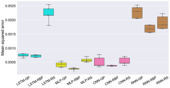
In Figure 1 we show the distribution of the optimal outer objective function values over five trials for all models and all optimization methods after the optimization has finished. The final mean squared errors (MSEs) are fairly low for all learning models and all optimization approaches. In the online supplement in Table 2, we show the numerical MSE values for all trials as well as the corresponding deviation of the predicted groundwater level from the truth. Almost all trials of all models reach a deviation of about 2 meters or less, which is considered highly accurate. Figure 1 shows that there is a noticeable difference between the performance of the types of learning models, with MLP and CNN generally leading to the smallest (best) final MSEs. We also observe a difference in the variation of the results over the five trials with RBF leading to the smallest variation for all HPO methods. The RNN performs worst regardless of the HPO method used. This may be related to the fact that all HPO methods have difficulties in finding optimal solutions or that the RNN is simply not able to capture the groundwater data any better. Figure 1 also indicates that the RBF approach generally leads to the lowest errors among all HPO methods.

Figure 1: Boxplots of mean squared errors for the single well case over five HPO trials. Low values are better. LSTM=long short-term memory network; MLP=multilayer perceptron; CNN=convolutional neural network; RNN=recurrent neural network; GP=Gaussian process; RBF=radial basis function; RS = random sampling.

Analysis of Optimized Hyperparameters

We compare the distributions of the final hyperparameter values over all five trials obtained with the different HPO methods. Figure 1 showed that the MLP optimized with the RBF approach leads overall to the best results. Figure 2 shows the corresponding hyperparameters. Here, the colored bars represent the mean and the black lines show the standard deviation over the five solutions for the MLP. We see that generally all HPO methods lead to a more complex MLP network, the RBF method leading to approximately 5 layers with approximately 25 nodes each. For the RBF method, the lag is large, using almost a full year of past data. The dropout rate and the optimal number of epochs for the RBF method are smaller than those obtained with the GP. Note that larger dropout rates discourage overfitting of the models to the data. We observe the largest differences between the HPO methods for the number of epochs.

The distributions of the optimal hyperparameters for LSTM, CNN, and RNN are shown in the online supplement in Section C.1.1 in Figure 3. For the CNN, we observe a similar behavior as for the MLP: the optimal RBF solutions have a large number of layers, filters, and lags. For LSTM, all HPO methods prefer smaller, less complex networks, and for the RNN, the HPO methods return networks of different complexities with generally larger standard deviations on the optimal hyperparameter values.

Figure 2: Distribution of the optimized hyperparameter values for MLP for the single well case. The colored bars represent the mean and the black lines show the standard deviation over five solutions. LSTM=long short-term memory network; MLP=multilayer perceptron; CNN=convolutional neural network; RNN=recurrent neural network; GP=Gaussian process; RBF=radial basis function; RS = random sampling.

Analysis of HPO Convergence

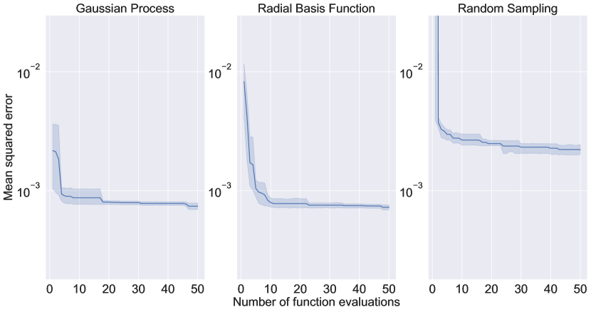
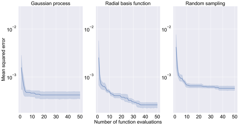
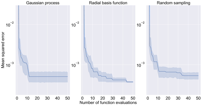
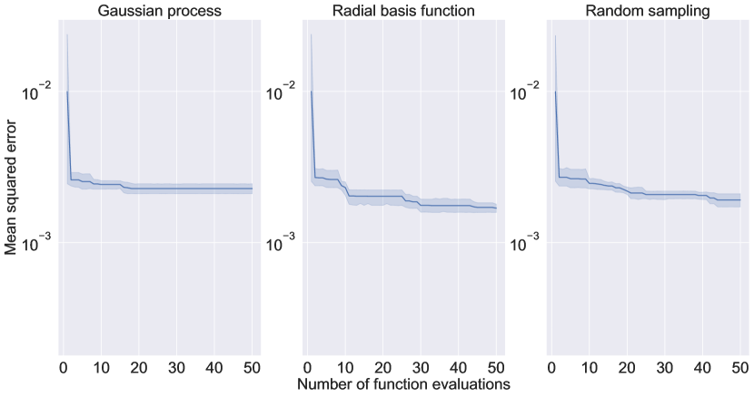
Besides the final solutions obtained with the different HPO methods, we are also interested in how fast the methods converge, i.e., how many calls to the inner optimization loop are necessary. For this purpose, we use progress plots that illustrate how quickly the average and the standard deviation of the outer objective function values over five trials decrease as the number of function evaluations increases. Ideally, the graphs should drop off fast, which means that improved network architectures were found within very few hyperparameter evaluations. The plot of the standard deviation reflects how robust each method is. Small standard deviation envelopes indicate that all five trials with the HPO methods converged to an approximately equally good solution. We show these convergence plots in Figure 3.

For the LSTM (Figures 3(a)) we can see that the GP and RBF approaches lead to more robust solutions (narrow standard deviation bands) than the RS approach. The standard deviation associated with the random sampling remains the largest throughout. This can be expected as the random sampling does not have a systematic search approach that allows it to intensify the search locally around good solutions.

For MLP, on the other hand, the RBF performed best and the convergence plot (Figure 3(b)) reflects that the RBF approach also converged faster than the GP and the RS. For MLP, GP has wider standard deviation bands than RBF throughout indicating less robustness. The standard deviations obtained with RS are smaller for MLP than for LSTM. Since the RS is lacking any systematic search for improvements, this may be an indicator that there are several solutions for MLP with similar performance.

For CNN (Figure 3(c)), we can see significant differences in the convergence behavior between the three HPO methods. The RBF approach has smaller standard deviations than GP and RS. We notice that the search with the GP gets stuck after about 12 function evaluations and it gets stuck in different solutions as is reflected by the width of the standard deviation envelopes.

Finally, for RNN (Figures 3(d)), we observe the overall worst performance. All HPO models make only slow progress towards improved solutions and the five trials with the RBF method show the average best performance.

(a) LSTM

(b) MLP

(c) CNN

(d) RNN

Figure 3: Convergence plots showing the average and the standard deviation of the outer objective function values over five trials versus the number of function evaluations for all four learning models for the single well case.

Analysis of Computing Times

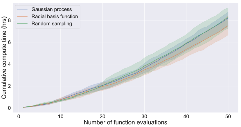
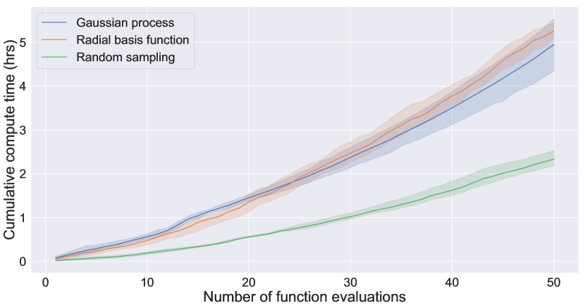
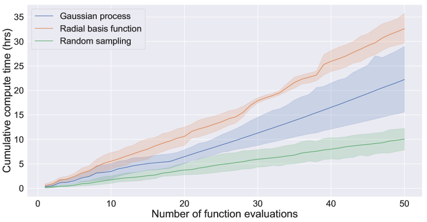
As training larger, more complex networks requires more compute time, we also plot the cumulative function evaluation time for each network type and each HPO method in order to compare the wall clock time to solution. Here, we only compare the amount of time spent on function evaluations and we assume that the HPO methods’ own computational overheads are negligible. We show the average and the standard deviations of the computing times over all five trials in Figure 4. Comparing the figures, we see that optimizing the hyperparameters of the MLP (Figure 4(b)) is fastest for all HPO methods (within 5 hours) even though the optimal MLP architectures were fairly complex.

For the LSTM (Figure 4(a)), we can see that the computing times of all three HPO methods are approximately equal. Since the final optimized networks are smaller compared to MLP for all HPO methods and the number of epochs is approximately the same for RS and GP (compare Figure 3a in Section C.1.1 in the online supplement), we conclude that on average all HPO methods tried networks of similar complexity. The computing times for the CNN (Figure 4(c)) are significantly larger than for all other network types (RBF needs on average over 30 hours for the CNN compared to less than 8 hours for all other network types). For RNN (Figure 4(d)), we observe large variations between the times for the individual optimization trials. RBF may take from 3 to 11 hours and RS takes between 7 hours and 25 hours. Thus, if the goal is to train learning models on a laptop or simple desktop computer to make predictions for future groundwater levels in a timely manner, one may prefer using the MLP or the LSTM in terms of expected computing time.

(a) LSTM

(b) MLP

(c) CNN

(d) RNN

Figure 4: Cumulative function evaluation time versus number of function evaluations for all four learning models for the single well case.

Analysis of Performance on Testing Data

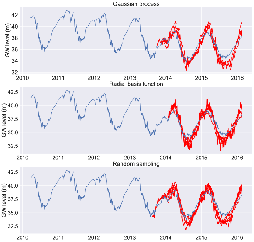
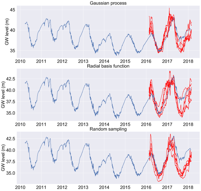
We illustrate in Figure 5 how well the optimized MLP and LSTM models capture the testing time series data (for CNN and RNN results, see the online supplement, Section C.1.2, Figure 4). As described earlier, we train the models on a subset of the historical observations (approximately beginning 2010-end 2013) and we test their performance on another subset (approximately beginning 2014-end 2015) to compute the outer objective function values. In Figures 5(a) and 5(b), we show the training data and for each optimization trial, we show the predictions of the optimized models for the testing data. The closer the predictions (red graphs) are to the true data (blue), the better. We can see that both MLP and LSTM are able to capture the seasonality in the data well. The predictions made with the MLP appear more erratic, i.e, we see many small jumps in daily groundwater predictions. This behavior is observed in the daily groundwater measurements and is due to, e.g., irrigation or other water withdrawal activities. The LSTM predictions are somewhat smoother, which indicates that the daily drawdown patterns are not learned as well.

(a) MLP

(b) LSTM

Figure 5: Groundwater level predictions obtained from five hyperparameter optimizations of MLP and LSTM, respectively, for the single well case for each HPO method. GW=groundwater.

Out-of-Sample Future Groundwater Predictions

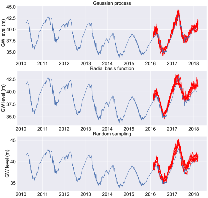
Finally, we are interested in how well the optimized learning models will predict groundwater data that was not used during the HPO. We retrain the models with the optimized hyperparameters on the whole dataset $\mathcal{D}$ (2010-2016) and we predict the groundwater levels from February 20, 2016 to February 28, 2018. We illustrate these “out-of-sample” predictions for each of the five trials for MLP and LSTM in Figure 6. We see that both models are able to keep the trend in the data (decreasing groundwater levels in the summer, increasing levels in the winter), but the MLP predictions are much more accurate and less variable than the LSTM predictions. The LSTM is not able to capture the higher groundwater levels in the wet years (2017, 2018). The out-of-sample predictions for CNN and RNN are provided in the online supplement in Section C.1.3 in Figure 5. The RNN makes significantly worse out-of-sample predictions than the MLP. The distributions of the MSEs for the out-of-sample predictions are provided in the form of boxplots in the online supplement in Figure 6.

(a) MLP

(b) LSTM

Figure 6: Out-of-sample groundwater predictions with the five optimized MLP and LSTM models, respectively, for the single well case. GW=groundwater.

5.6 Results for Predicting Groundwater at Multiple Wells in Butte County, CA

Watersheds are large and generally have more than a single well from which groundwater is pumped or with the help of which the amount of available groundwater is monitored. Using multiple wells will allow us to better assess the average health of a watershed, and thus to avoid letting local fluctuations drive policies and decisions. Therefore, within Butte County, we selected three additional wells. Ideally, we do not want to train and optimize a separate learning model for each well, but rather we want one learning model that can be trained on and used for predicting the data at multiple wells simultaneously. We train and optimize the hyperparameters as before with the only difference that we now have three groundwater input data streams and three nodes in each output layer. We use these data to optimize the hyperparameters of MLP, LSTM, and CNN. For reasons of space considerations, we present detailed results only for the MLP. The LSTM and CNN results are in the online supplement in Section C.2.

Comparison of Mean Squared Errors

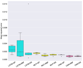
We show a comparison of the distributions of the final mean squared errors for all three learning models and all HPO methods obtained from five optimization trials in Figure 7. The optimal mean squared errors are for almost all models and HPO methods larger by an order of magnitude for the multi-well case than for the single well case (see also the numerical data provided in Table 3 in the online supplement). This is to be expected as more time series must be fit and one set of hyperparameters may not be optimal for the data of all three wells. We can see that the MLP and the CNN optimized with the RBF approach lead to the lowest errors. Also RS performs reasonably well for all three models in the multi-well case, while it showed significantly worse performance in the single well case. Thus, in terms of performance consistency, one should opt for an HPO method that systematically explores the search space rather than the RS method.

Figure 7: Boxplots of mean squared errors for the multi-well case. LSTM=long short-term memory network; MLP=multilayer perceptron; CNN=convolutional neural network; RNN=recurrent neural network; GP=Gaussian process; RBF=radial basis function; RS = random sampling.

Analysis of Optimized Hyperparameters

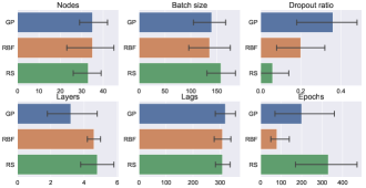
We show the distribution of the optimized hyperparameters only for the MLP (Figure 8). The results for LSTM and CNN are in the online supplement in Section C.2.1 in Figure 7. For the MLP, the RBF method chooses again a large complex network (4-5 layers and on average over 30 nodes per layer) and a large lag. Also the optimal solutions for the CNN (see online supplement) show that a complex network with many layers and filters is preferred and also the lag is large. On the other hand, the optimal LSTM network structure is significantly smaller with only 1-2 layers.

Figure 8: Distribution of the optimized hyperparameter values for MLP for the multi-well case. The colored bars show the mean of the values over five trials and the black lines indicate the standard deviation. GP=Gaussian process; RBF=radial basis function; RS=random sampling.

Analysis of HPO Convergence

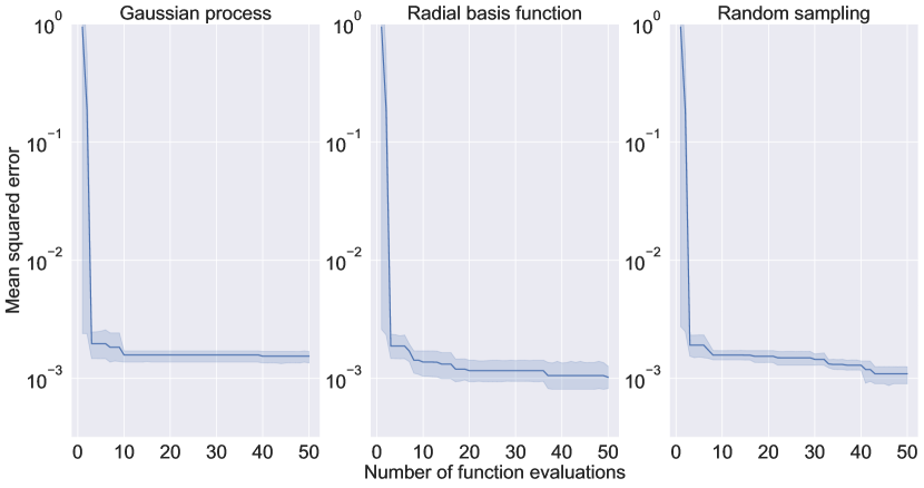
As for the single well case, we illustrate how fast each HPO method converges. We show the progress plots on the example of MLP in Figure 9(a) (results for LSTM and CNN are in the online supplement in Section C.2.2 in Figure 8). We observe that all HPO methods converge fast and the RBF method achieves on average the best performance.

Analysis of Computing Times

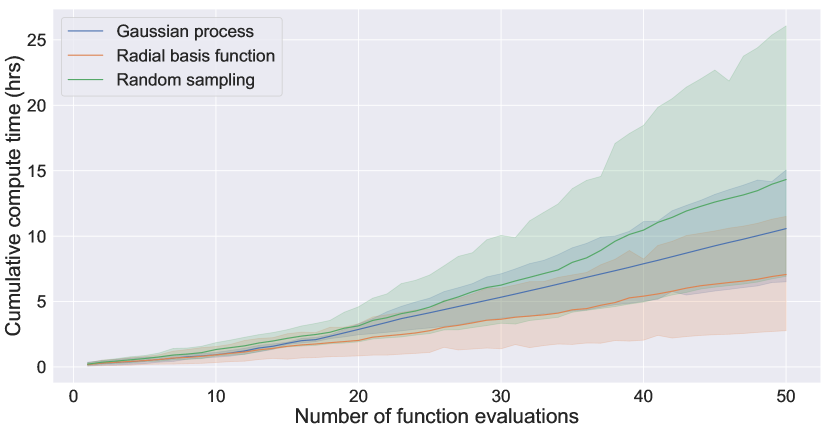
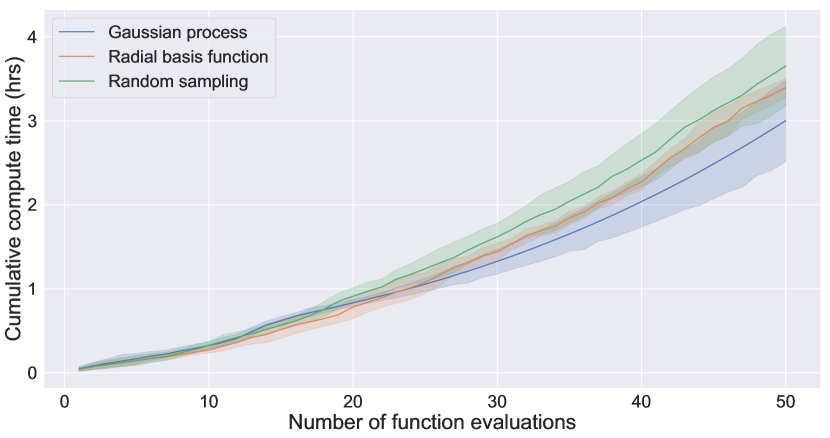
The cumulative computation time for the MLP over all function evaluations is shown in Figure 9(b). All HPO methods require approximately the same time and the HPO is completed within 4 hours. The CNN again requires the largest amount of time to solution (up to 30 hours) and the HPO for the LSTM completes within 10 hours (see Figure 10 in Section C.2.4 in the online supplement). Thus, we conclude that the MLP optimized with the RBF should be the learning model and HPO method of choice as it attains high quality solutions within the lowest computation time.

(a) Convergence plot

(b) Cumulative evaluation time

Figure 9: Convergence plot showing the average and the standard deviation of the outer objective function value versus the number of function evaluations (left) and cumulative function evaluation time versus number of function evaluations (right) for MLP for the multiple well case.

Analysis of Performance on Testing Data

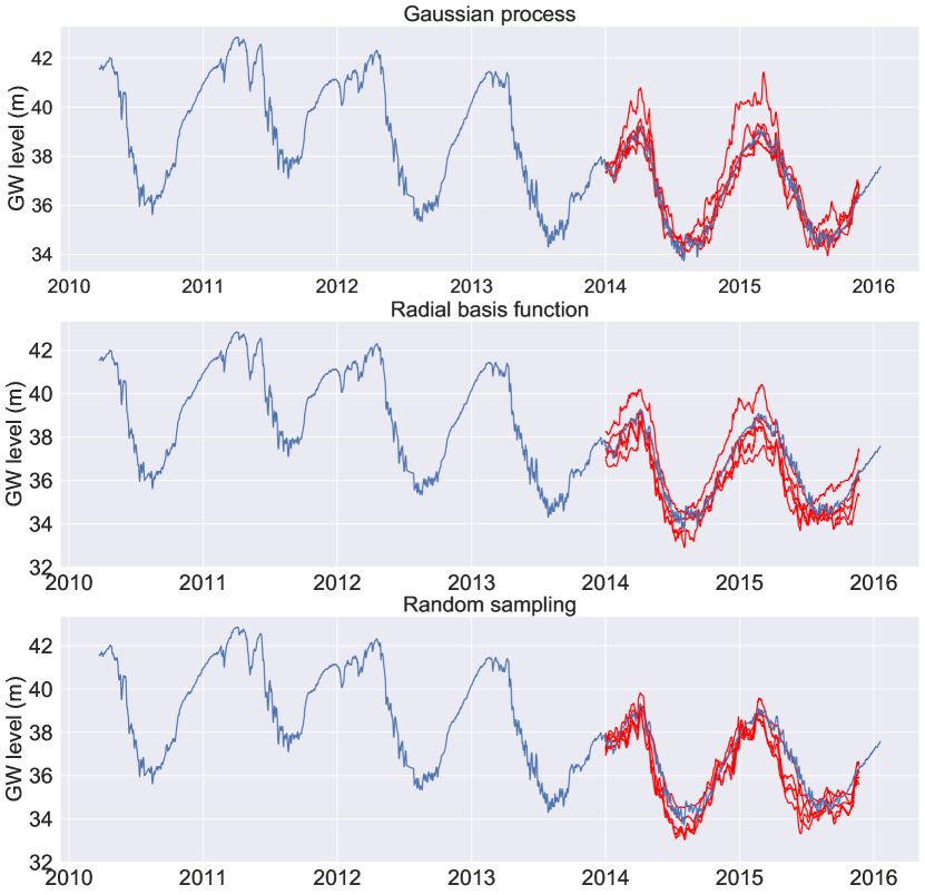
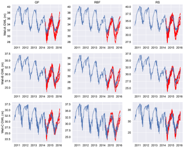
In Figure 10, we show the predictions obtained with the optimized MLP models for all three wells for the testing data. All three HPO methods are able to capture the seasonality in the data and all three HPO methods appear to underpredict the true groundwater levels for wells A and B. Well C is generally better fitted by all three HPO methods. This same observation holds true for the CNN predictions (Figure 9b in Section C.2.3 in the online supplement). One possible explanation is that the errors made in the predictions for well C dominate the HPO. This may be due to the more erratic behavior of the groundwater levels for well C, which are manifested by more severe drawdowns and thus more patterns must be learnt (the most complex time series dominated the optimization). Using a weighted sum of the wells’ errors as outer objective function could potentially help mitigating this problem. The LSTM predictions (Figure 9a in Section C.2.3 in the online supplement) have generally a larger variability than CNN and MLP and we observe larger jumps in the daily groundwater predictions. Note that for the multi-well case, we do not have additional observations for all three wells for making “out-of-sample” predictions.

Figure 10: Groundwater level predictions obtained from five hyperparameter optimizations of MLP for the multiple well case for each HPO method. GWL=groundwater level.

6 Summary and Directions of Future Research

Our work presented in this article is motivated by the need for computationally lightweight approximation models that can run on a laptop or simple desktop computer and that can reasonably accurately predict groundwater levels with the overarching goal to enable timely and reliable water resources management decisions.

In this article, we studied the applicability of several purely data-informed learning models whose hyperparameters were optimized with three different methods for predicting the groundwater level. We used four deep learning models, namely convolutional neural networks (CNNs), recurrent neural networks (RNNs), multilayer perceptron (MLP), and long short-term memory networks (LSTMs). We formulated a bilevel optimization problem for finding the optimal hyperparameters of the learning models. At the upper level, we have a pure-integer stochastic problem, and at the lower level, we have a large-scale global optimization problem. We solved the hyperparameter optimization (HPO) problem with three different methods. We used two surrogate model based optimization methods (one based on radial basis functions (RBFs) and one based on Gaussian process (GP) models) and a random sampling method. In our numerical experiments, we trained the learning models on daily observation data of groundwater levels and meteorological variables at, respectively, one (“single well case”) and three (“multi-well case”) groundwater monitoring wells in Butte County, California, USA.

Our study shows that with the right HPO method, different types of deep learning models, including CNN, LSTM, and MLP (and to a limited extend also RNN), can be tuned to make accurate forecasts of daily groundwater levels (within two meters of the true values). The main difference between the performance of the methods is the total optimization time and the associated optimal model complexity. We showed that the surrogate model based HPO methods lead to better performing network architectures than randomly sampling the hyperparameter space. Our results show that the “simplest” learning model, the MLP, optimized with the RBF method, generally performs best and its optimization time is lowest. The RNN is the worst performing model and the most cumbersome to use as it often fails to fit a model for an architecture due to its problems during backpropagation. The CNN also performs well in terms of prediction accuracy, but it requires considerably more computation time than the other models. The results for the LSTM are less robust and have a large variation.

Directions of future research include applying the RBF-optimized MLP model for groundwater predictions at other watersheds in California and other parts of the United States to assess how well our method generalizes to watersheds with different characteristics (e.g., geology, groundwater use, weather patterns). We will study the sensitivity of the model performance to different input variables. This analysis will inform us about which data should be collected and thus where the necessary data acquisition infrastructure investments should be made. Similarly, we will study how sensitive the model predictions are to the amount of training data points (daily versus monthly observations) and when fewer years of data are used in training. This future research direction also includes applying our method for learning model optimization on other time series data such as predicting water quality.

Acknowledgements

This work was supported by Laboratory Directed Research and Development (LDRD) funding from Berkeley Lab, provided by the Director, Office of Science, of the U.S. Department of Energy under Contract No. DE-AC02-05CH11231. This research used resources of the National Energy Research Scientific Computing Center (NERSC), a U.S. Department of Energy Office of Science User Facility operated under Contract No. DE-AC02-05CH11231.

References

- [1] Y. LeCun, Y. Bengio, and G. Hinton. Deep learning. Nature, 521(436-444), 2015.
- [2] M. Kuderer, S. Gulati, and W. Burgard. Learning driving styles for autonomous vehicles from demonstration. In 2015 IEEE International Conference on Robotics and Automation (ICRA), pages 2641–2646, 2015.
- [3] S. Rudy, A. Alla, S.L. Brunton, and J.N. Kutz. Data-driven identification of parametric partial differential equations. SIAM Journal on Applied Dynamical Systems, 18(2):643–660, 2019.
- [4] L. Bottou. Large-scale machine learning with stochastic gradient descent. In 19th International Conference on Computational Statistics, pages 177–186, 2010.
- [5] H. Robbins and S. Monro. A stochastic approximation method. The Annals of Mathematical Statistics, 22(3):400–407, 1951.
- [6] D.P. Kingma and J.L. Ba. ADAM: A method for stochastic optimization. In ICLR 2015, 2015.
- [7] A. Najah, A. El-Shafie, O.A. Karim, and A.H. El-Shafie. Application of artificial neural networks for water quality prediction. Neural Computing and Applications, 22(1):187–201, 2013.
- [8] J. Zhang, Y. Zhu, X. Zhang, M. Ye, and J. Yang. Developing a Long Short-Term Memory (LSTM) based model for predicting water table depth in agricultural areas. Journal of Hydrology, 561(918-929), 2018.
- [9] J. Bergstra and Y. Bengio. Random search for hyper-parameter optimization. The Journal of Machine Learning Research, 13(1):281–305, 2012.
- [10] I. Ilievski, T. Akhtar, J. Feng, and C.A. Shoemaker. Efficient hyperparameter optimization of deep learning algorithms using deterministic RBF surrogates. In Proceedings of the Thirty-First AAAI Conference on Artificial Intelligence, 2017.
- [11] J. Snoek, H. Larochelle, and R. P. Adams. Practical Bayesian optimization of machine learning algorithms. In Advances in Neural Information Processing Systems, 2012.
- [12] J. Bergstra, D. Yamins, and D.D. Cox. Making a science of model search: Hyperparameter optimization in hundreds of dimensions for vision architectures. In Proceedings of the 30th International Conference on Machine Learning, 2013.
- [13] A. Klein, S. Falkner, S. Bartels, P. Hennig, and F. Hutter. Fast Bayesian optimization of machine learning hyperparameters on large datasets. In Proceedings of the 20th International Conference on Artificial Intelligence and Statistics (AISTATS) 2017, Fort Lauderdale, Florida, USA, volume 54, 2017.
- [14] H. Jin, Q. Song, and X. Hu. Auto-Keras: An efficient neural architecture search system. arXiv preprint arXiv:1806.10282 [cs.LG], 2019.
- [15] S.R. Young, D.C. Rose, T.P. Karnowski, S.-H. Lim, and R.M. Patton. Optimizing deep learning hyper-parameters through an evolutionary algorithm. In MLHPC ’15 Proceedings of the Workshop on Machine Learning in High-Performance Computing Environments, volume Article No.4, 2015.
- [16] D. Lakhmiri, S. Le Digabel, and C. Tribes. HyperNOMAD: Hyperparameter optimization of deep neural networks using mesh adaptive direct search. arXiv preprint arXiv:1907.01698 [cs.LG], July 2019.
- [17] S. Le Digabel. Algorithm 909: NOMAD: Nonlinear optimization with the MADS algorithm. ACM Transactions on Mathematical Software, 37, 2011.
- [18] P. Balaprakash, M. Salim, T.D. Uram, V. Vishwanath, and S.M. Wild. Deephyper: Asynchronous hyperparameter search for deep neural networks. In 2018 IEEE 25th International Conference on High Performance Computing (HiPC), pages 42–51, 2018.
- [19] C. Audet and M. Kokkolaras. Blackbox and derivative-free optimization: theory, algorithms and applications. Optimization and Engineering, 17(1):1–2, 2016.
- [20] A.J. Booker, J.E. Dennis Jr, P.D. Frank, D.B. Serafini, V. Torczon, and M.W. Trosset. A rigorous framework for optimization of expensive functions by surrogates. Structural Multidisciplinary Optimization, 17:1–13, 1999.
- [21] H.-M. Gutmann. A radial basis function method for global optimization. Journal of Global Optimization, 19:201–227, 2001.
- [22] R.G. Regis and C.A. Shoemaker. A stochastic radial basis function method for the global optimization of expensive functions. INFORMS Journal on Computing, 19:497–509, 2007.
- [23] K. Holmström. An adaptive radial basis algorithm (ARBF) for expensive black-box global optimization. Journal of Global Optimization, 41:447–464, 2008.
- [24] D.R. Jones, M. Schonlau, and W.J. Welch. Efficient global optimization of expensive black-box functions. Journal of Global Optimization, 13:455–492, 1998.
- [25] C. Audet and J.E. Dennis Jr. Mesh adaptive direct search algorithms for constrained optimization. SIAM Journal on Optimization, 17:188–217, 2006.
- [26] J. Müller and J. Woodbury. GOSAC: global optimization with surrogate approximation of constraints. Journal of Global Optimization, doi:10.1007/s10898-017-0496-y, 2017.
- [27] L. Nuñez, R.G. Regis, and K. Varela. Accelerated random search for constrained global optimization assisted by radial basis function surrogates. Journal of Computational and Applied Mathematics, 340:276–295, 2018.
- [28] R.G. Regis. Stochastic radial basis function algorithms for large-scale optimization involving expensive black-box objective and constraint functions. Computers & Operations Research, 38:837–853, 2011.
- [29] J. Müller, C.A. Shoemaker, and R. Piché. SO-I: a surrogate model algorithm for expensive nonlinear integer programming problems including global optimization applications. Journal of Global Optimization, 59:865–889, 2013.
- [30] M.A. Abramson, C. Audet, J. Chrissis, and J. Walston. Mesh adaptive direct search algorithms for mixed variable optimization. Optimization Letters, 3:35–47, 2009.
- [31] E. Davis and M. Ierapetritou. Kriging based method for the solution of mixed-integer nonlinear programs containing black-box functions. Journal of Global Optimization, 43:191–205, 2009.
- [32] K. Holmström. An adaptive radial basis algorithm (ARBF) for expensive black-box mixed-integer global optimization. Journal of Global Optimization, 9:311–339, 2008.
- [33] J. Müller. MISO: Mixed integer surrogate optimization framework. Optimization and Engineering, 17(1):177–203, 2015.
- [34] J. Müller, C.A. Shoemaker, and R. Piché. SO-MI: A surrogate model algorithm for computationally expensive nonlinear mixed-integer black-box global optimization problems. Computers and Operations Research, 40:1383–1400, 2013.
- [35] R. Datta and R.G. Regis. A surrogate-assisted evolution strategy for constrained multi-objective optimization. Expert Systems with Applications, 57:270–284, 2016.
- [36] J. Müller. SOCEMO: Surrogate Optimization of Computationally Expensive Multiobjective Problems. INFORMS Journal on Computing, 29(4):581–596, 2017.
- [37] R. Gramacy and S. Le Digabel. The mesh adaptive direct search algorithm with treed Gaussian process surrogates. Pacific Journal of Optimization, 11, 2011.
- [38] H.K.H. Lee, R.B. Gramacy, C. Linkletter, and G.A. Gray. Optimization subject to hidden constraints via statistical emulation. Pacific Journal of Optimization, 7:467–478, 2011.
- [39] J. Müller and M. Day. Surrogate optimization of computationally expensive black-box problems with hidden constraints. INFORMS Journal on Computing, Articles in Advance 05 Jul 2019(https://doi.org/10.1287/ijoc.2018.0864), 2019.
- [40] C. Audet, G. Savard, and W. Zghal. A mesh adaptive direct search algorithm for multiobjective optimization. European Journal of Operational Research, 204(3):545–556, 2010.
- [41] J. Müller. An algorithmic framework for the optimization of computationally expensive bi-fidelity black-box problems”. INFOR: Information Systems and Operational Research, DOI: 10.1080/03155986.2019.1607810, 2019.
- [42] A.I.J. Forrester, A. Sóbester, and A.J. Keane. Multi-fidelity optimization via surrogate modelling. Proceedings of the Royal Society, 463:3251–3269, 2007.
- [43] C. Audet and W. Hare. Derivative-Free and Blackbox Optimization. Springer Series in Operations Research and Financial Engineering, Springer International Publishing, 2017.
- [44] O. Karslıoğlu, M. Gehlmann, J. Müller, S. Nemšàk, J. Sethian, A. Kaduwela, H. Bluhm, and C. Fadley. An efficient algorithm for automatic structure optimization in X-ray standing-wave experiments. Journal of Electron Spectroscopy and Related Phenomena, 230:10–20, 2019.
- [45] W. Langhans, J. Müller, and W. Collins. Optimization of the Eddy‐Diffusivity/Mass‐Flux shallow cumulus and boundary‐layer parameterization using surrogate models. Journal of Advances in Modeling Earth Systems, 11:402–416, 2019.
- [46] J. Müller, R. Paudel, C.A. Shoemaker, J. Woodbury, Y. Wang, and N. Mahowald. CH4 parameter estimation in CLM4.5bgc using surrogate global optimization. Geoscientific Model Development Discussions, 8:141–207, 2015.
- [47] D. Toal and A. Keane. Efficient multi-point aerodynamic design optimization via co-kriging. Journal of Aircraft, 48(5):1685–1695, 2011.
- [48] G. Matheron. Principles of geostatistics. Economic Geology, 58:1246–1266, 1963.
- [49] M.J.D. Powell. Advances in Numerical Analysis, vol. 2: wavelets, subdivision algorithms and radial basis functions. Oxford University Press, Oxford, pp. 105-210, chapter The Theory of Radial Basis Function Approximation in 1990. Oxford University Press, London, 1992.
- [50] M.J.D. Powell. Recent Research at Cambridge on Radial Basis Functions. New Developments in Approximation Theory, pp. 215-232. Birkhäuser, Basel, 1999.
- [51] R.H. Myers and D.C. Montgomery. Response Surface Methodology, Process and Product Optimization using Designed Experiments. Wiley-Interscience Publication, 1995.
- [52] S.M. Wild and C.A. Shoemaker. Global convergence of radial basis function trust-region algorithms for derivative-free optimization. SIAM Review, 55:349–371, 2013.
- [53] M. Mitchell. An Introduction to Genetic Algorithms. Cambridge, MA: MIT Press, 1996.
- [54] D.E. Rumelhart, G.E. Hinton, R.J. Williams, et al. Learning representations by back-propagating errors. Cognitive modeling, 5(3):1, 1988.
- [55] G. Hinton, N. Srivastava, and K. Swersky. Neural networks for machine learning. lecture 6a, overview of mini-batch gradient descent. lecture notes, 2012.
- [56] C.M. Bishop et al. Neural networks for pattern recognition. Oxford University Press, 1995.
- [57] S. Trenn. Multilayer perceptrons: Approximation order and necessary number of hidden units. IEEE transactions on neural networks, 19(5):836–844, 2008.
- [58] Z. Ali, I. Hussain, M. Faisal, H.M. Nazir, T. Hussain, M.Y. Shad, A. Mohamd Shoukry, and S. Hussain Gani. Forecasting drought using multilayer perceptron artificial neural network model. Advances in Meteorology, ID 5681308:9 pages, 2017.
- [59] H. Tabari and P.H. Talaee. Multilayer perceptron for reference evapotranspiration estimation in a semiarid region. Neural Computing and Applications, 23(2):341–348, 2013.
- [60] P. Araujo, G. Astray, J.A. Ferrerio-Lage, J.C. Mejuto, J.A. Rodriguez-Suarez, and B. Soto. Multilayer perceptron neural network for flow prediction. Journal of Environmental Monitoring, 13(1):35–41, 2011.
- [61] M.W. Gardner and S.R. Dorling. Artificial neural networks (the multilayer perceptron) – a review of applications in the atmospheric sciences. Atmospheric Environment, 32(14-15):2627–2636, 1998.
- [62] Y. LeCun, L. Bottou, Y. Bengio, P. Haffner, et al. Gradient-based learning applied to document recognition. Proceedings of the IEEE, 86(11):2278–2324, 1998.
- [63] K. He, X. Zhang, S. Ren, and J. Sun. Deep residual learning for image recognition. In Proceedings of the IEEE Conference on Computer Vision and Pattern Recognition, pages 770–778, 2016.
- [64] Z. Cui, W. Chen, and Y. Chen. Multi-scale convolutional neural networks for time series classification. arXiv preprint arXiv:1603.06995, 2016.
- [65] A. Borovykh, S. Bohte, and C.W. Oosterlee. Conditional time series forecasting with convolutional neural networks. arXiv preprint arXiv:1703.04691, 2017.
- [66] T. Mikolov, M. Karafiát, L. Burget, J. Černockỳ, and S. Khudanpur. Recurrent neural network based language model. In Eleventh Annual Conference of the International Speech Communication Association, 2010.
- [67] I. Sutskever, J. Martens, and G.E. Hinton. Generating text with recurrent neural networks. In Proceedings of the 28th International Conference on Machine Learning (ICML-11), pages 1017–1024, 2011.
- [68] Y.-M. Chiang, L.-C. Chang, and F.-J. Chang. Comparison of static-feedforward and dynamic-feedback neural networks for rainfall–runoff modeling. Journal of Hydrology, 290(3-4):297–311, 2004.
- [69] P. Coulibaly, F. Anctil, R. Aravena, and B. Bobée. Artificial neural network modeling of water table depth fluctuations. Water Resources Research, 37(4):885–896, 2001.
- [70] S. Hochreiter and J. Schmidhuber. Long short-term memory. Neural Computing, 9:1735–1780, 1997.
- [71] F.A. Gers, J. Schmidhuber, and F. Cummins. Learning to forget: continual prediction with LSTM. Neural Computing, 12:2451–2471, 2000.
- [72] M. Sundermeyer, R. Schluter, and H. Ney. LSTM neural networks for language modeling. In Proceedings of the 12th Annual Conference of the International Speech Communication Association, Portland, Oregon, USA, pages 601–608, 2012.
- [73] A. Graves, A. Mohamed, and G. Hinton. Speech recognition with deep recurrent neural networks. In Proceedins of the 2013 International Conference on Acoustics, Speech, and Signal Processing, 2013.
- [74] X. Ma, Z. Tao, Y. Wang, H. Yu, and Y. Wang. Long short-term memory neural network for traffic speed prediction using remote microwave sensor data. Transportation Research Part C: Emerging Technologies, 54:187–197, 2015.
- [75] D. Hsu. Multi-period time series modeling with sparsity via Bayesian variational inference. arXiv preprint arXiv:1707.00666v3, 2018.
- [76] California Department of Water Resources. SGMA groundwater management.
- [77] B.I. Cook, J.S. Mankin, and K.J. Anchukaitis. Climate change and drought: From past to future. Current Climate Change Reports, 4(2):164–179, 2018.
- [78] M Taylor. Liquid Assets: Improving management of the state’s groundwater resources. Technical report, Legislative Analyst’s Office, 2010.
- [79] C.D. Langevin, J.D. Hughes, E.R. Banta, R.G. Niswonger, S. Panday, and A.M. Provost. Documentation for the MODFLOW 6 groundwater flow model. Technical report, US Geological Survey, 2017.
- [80] C.I. Steefel, C.A.J. Appelo, B. Arora, D. Jacques, T. Kalbacher, O. Kolditz, V. Lagneau, P.C. Lichtner, K.U. Mayer, J.C.L. Meeussen, et al. Reactive transport codes for subsurface environmental simulation. Computational Geosciences, 19(3):445–478, 2015.
- [81] T. Xu, N. Spycher, E. Sonnenthal, G. Zhang, L. Zheng, and K. Pruess. TOUGHREACT version 2.0: A simulator for subsurface reactive transport under non-isothermal multiphase flow conditions. Computers & Geosciences, 37(6):763–774, 2011.
- [82] S. Sahoo, T.A. Russo, J. Elliott, and I. Foster. Machine learning algorithms for modeling groundwater level changes in agricultural regions of the US. Water Resources Research, 53(5):3878–3895, 2017.
- [83] F. Karandish and J. Šimunek. A comparison of numerical and machine-learning modeling of soil water content with limited input data. Journal of Hydrology, 543:892–909, 2016.
- [84] I.N. Daliakopoulos, P. Coulibaly, and I.K. Tsanis. Groundwater level forecasting using artificial neural networks. Journal of Hydrology, 309(1-4):229–240, 2005.
- [85] F. Kratzert, D. Klotz, C. Brenner, K. Schulz, and M. Herrnegger. Rainfall–runoff modelling using long short-term memory (LSTM) networks. Hydrology and Earth System Sciences, 22(11):6005–6022, 2018.
- [86] C.C. Faunt. Groundwater availability of the Central Valley aquifer, California. Professional paper 1766, 225 p., U.S. Geological Survey, 2009.
- [87] S. Moritz and T. Bartz-Beielstein. imputeTS: Time series missing value imputation in R. 2017.
- [88] F. Chollet. keras. GitHub repository, https://github.com/fchollet/keras, 2015.
- [89] M. Abadi, A. Agarwal, P. Barham, E. Brevdo, Z. Chen, C. Citro, G.S. Corrado, A. Davis, J. Dean, M. Devin, et al. Tensorflow: Large-scale machine learning on heterogeneous distributed systems. arXiv preprint arXiv:1603.04467, 2016.
- [90] F.-A. Fortin, F.-M. De Rainville, M.-A. Gardner, C. Gagné, and M. Parizeau. DEAP: Evolutionary algorithms made easy. Journal of Machine Learning Research, 13:2171–2175, 2012.
- [91] F. Pedregosa, G. Varoquaux, A. Gramfort, V. Michel, B. Thirion, O. Grisel, M. Blondel, P. Prettenhofer, R. Weiss, V. Dubourg, J. Vanderplas, A. Passos, D. Cournapeau, M. Brucher, M. Perrot, and E. Duchesnay. Scikit-learn: Machine learning in Python. Journal of Machine Learning Research, 12:2825–2830, 2011.