Harnessing symmetry-protected topological order for quantum memories

Abstract

Spin chains with symmetry-protected edge modes are promising candidates to realize intrinsically robust physical qubits that can be used for the storage and processing of quantum information. In any experimental realization of such physical systems, weak perturbations in the form of induced interactions and disorder are unavoidable and can be detrimental to the stored information. At the same time, the latter may in fact be beneficial; for instance by deliberately inducing disorder which causes the system to localize. In this work, we explore the potential of using an $XZX$ cluster Hamiltonian to encode quantum information into the local edge modes and comprehensively investigate the influence of both many-body interactions and disorder on their stability over time, adding substance to the narrative that many-body localization may stabilize quantum information. We recover the edge state at each time step, allowing us to reconstruct the quantum channel that captures the locally constrained out of equilibrium time evolution. With this representation in hand, we analyze how well classical and quantum information are preserved over time as a function of disorder and interactions. We find that the performance of the edge qubits varies dramatically between disorder realizations. Whereas some show a smooth decoherence over time, a sizeable fraction are rapidly rendered unusable as memories. We also find that the stability of the classical information – a precursor for the usefulness of the chain as a quantum memory – depends strongly on the direction in which the bit is encoded. When employing the chain as a genuine quantum memory, encoded qubits are most faithfully recovered for low interaction and high disorder.

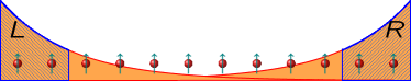
Figure 1: This is a sketch of the one-dimensional spin chain investigated in this work. The support of the edge zero mode operators under the influence of perturbations is depicted in orange. The blue regions are the local edge qubits to which an experimenter would have access.

I Introduction

The prospect of highly controllable quantum simulators Gross and Bloch (2017); Blatt and Roos (2012); Aspuru-Guzik and Walther (2012); Eisert et al. (2015) allows for the simulation of complex Hamiltonians, potentially realizing exotic phases of matter. A celebrated class of such phases are topological phases of matter which offer the promise of robust encodings of quantum information with a reduced need for active error correction Dennis et al. (2002); Kitaev (2003); Kitaev and Preskill (2006). Simple instances of these exist in one-dimensional spin chains, where one finds symmetry-protected topological phases (SPTs) which host emergent edge zero modes that enforce approximate degeneracies in the spectrum and define edge states which are dynamically decoupled from the bulk Haldane (1983); Kitaev (2001); Verresen et al. (2017); Wen (2013); Chen et al. (2013). The latter feature makes these systems interesting candidates for physical qubits used in quantum memories, as well as in implementations of measurement-based quantum computation Miller and Miyake (2015); Stephen et al. (2017); Raussendorf et al. (2017), which exploit the entanglement properties of the SPT to effectuate gate operations. However, for a practical quantum memory architecture, the topologically facilitated isolation of the edge states from the bulk must preserve the encoded data for a sufficiently long time, ideally several thousand multiples of the time taken to implement logical gates.

The ability of an SPT edge mode to retain information depends largely on the strength of interactions which perturb the SPT order. These drive two related phenomena: the splitting of the ground state degeneracy and the broadening of its edge zero modes. While the former controls the phase transition, the latter can have a significant impact on our ability to practically use the edge modes for storage purposes. We should typically expect to encode information into only a finite number of spins located at the boundary of the chain. The edge mode has no such restriction, and usually decays exponentially into the chain (see Fig. 1). This mismatch between the finite number of sites we can encode into and the long tails of the edge mode operators means that we can never expect our information to be totally preserved even when we take the system to the thermodynamic limit to make the edge modes exact constants of motion. With this in mind, one naturally turns to search for features which can further localize the edge modes without engaging in fine-tuning.

One readily available and promising candidate for this role is disorder. While usually considered an obstacle to analytical and numerical study, this feature is both generically present in physical systems and also enables a variety of localization phenomena, which may conceivably enhance the localization of the emergent edge modes. These go by different names depending on whether the underlying physics is describable using free fermions (Anderson localization Anderson (1958)) or is intrinsically interacting (many-body localization, abbreviated to MBL Abanin et al. (2019); Gogolin and Eisert (2016)). While the exact phenomenology of these two differ, both of those feature local constants of motion. In the SPT context this has been proposed as a method to attenuate the effective interaction between the two edge modes, since any coupling between them must be mediated by bulk eigenstates which, if only locally supported, can only connect the two via a prohibitively small number of virtual processes Huse et al. (2013); Chandran et al. (2014); Kjäll et al. (2014).

While this heuristic is appealing, precious little confirmation of it has been forthcoming since initial investigations established that the edge modes are not de-stabilized by the presence of disorder Bahri et al. (2015). In fact, a recent work by some of the authors Goihl et al. (2019) – built on the earlier Ref. Goihl et al. (2018) – suggests that the shape of the edge mode when subjected to disorder and interaction changes in a more intricate way than expected . There, the support of the edge modes was investigated and, surprisingly, found to depend heavily on the specific edge mode that was analysed. In light of this, a thorough examination of disorder effects on the temporal stability of edge mode appears to be urgently required. Here, achieve this goal: We explicitly determine the dynamics of the encoded subspace and quantify the extent to which information can be recovered at a given time.

Before proceeding, it is critical to specify what is meant by a good quantum memory. Any imperfect memory device can be viewed as a partially decohering channel acting upon the encoded quantum states. For a comprehensive investigation, the first step is to compute the operators that define this channel, from which all potentially relevant measures can then be calculated. It is important to carefully select measures that meaningfully quantify the notion of information preservation in the context of quantum computation and communication applications. Ideally, a measure should be operationally well motivated, straightforward to calculate and amenable to experimental verification. In this work, we perform full reconstruction of the time-evolved state on the edge mode subspace. This allows us to fully reconstruct the effective quantum channel applied at each time step. With this reconstruction at hand, we compute bounds on two measures of information preservation when using the system as a quantum memory: the retrievability of a logical bit, which is a prerequisite for a quantum memory; and the coherent information, which bounds the quantum capacity, that is the ultimate limit to quantum information transmission and particularly relevant for quantum communication applications, e.g., quantum repeaters Briegel et al. (1998); Muralidharan et al. (2016). For the classical information, we find a multi-faceted behaviour consistent with Ref. Goihl et al. (2019) supporting the observation that encoding with different edge state bases results in different stability behaviour. In the quantum information setting, we find that disorder helps the recovery of the encoded qubits, but low interaction strength is mandatory. Our results extend and enrich the narrative of disorder helping localize edge modes, as we find that there are encodings and Hamiltonian parameters for which this paradigm holds and others where it does not. In practice, this either makes an optimization over all possible parameters necessary to find the “sweet spot” of information coherence or demands an educated choice of physical realization. One can equally see our work as shedding new lights into notions of locally constrained non-equilibrium dynamics that interplays with disorder Chen et al. (2018).

II Setting

In this work, we analyze the interplay of disorder, interactions and symmetry-protected topological (SPT) order. We are specifically interested in the stability of the protected subspace spanned by the unperturbed edge modes when the system is subjected to many-body interactions and disorder. To measure the extent to which the locally encoded state gets entangled with the bulk, we time evolve the system and reconstruct the unperturbed edge mode subspace. We study a spin chain of length $N$ hosting a disordered $XZX$ cluster Hamiltonian

$$H_{0}(\{h_{j}\})=-\sum_{j=2}^{N-1}(1+h_{j})X_{j-1}Z_{j}X_{j+1}\,,$$ (1)

where the $h_{j}$ are drawn uniformly from the interval $[-\frac{\Delta}{2},\frac{\Delta}{2}]$ and $X_{j},Y_{j},Z_{j}$ are the Pauli operators acting at site $j$. Here, we restrict the disorder to act only on the cluster terms, disordering around a mean bulk gap of 1. We include this offset to distinguish the ability of disorder to help localize the edge modes from the bulk energy gap’s power to do the same. The choice to have disorder appear in the coefficient of the cluster terms is a pragmatic one; any other model of disorder, e.g. a random local magnetic field, competes with the SPT order and thereby drives a transition to a topologically trivial phase Huse et al. (2013); Bahri et al. (2015). Disordering the cluster terms themselves is an ideal version of disorder in the sense that this version splits degenerate levels for excited states, while preserving the ground state manifold. Therefore, we expect any other model of disorder to cause less localization in the system.

Even disordered, the Hamiltonian in Eq. (1) is a solvable representative of an SPT phase protected by the time reversal operator

$$\mathcal{T}=\prod_{i=1}^{N}Z_{i}\mathcal{K}\,,$$ (2)

where $\mathcal{K}$ is complex conjugation. Thus, this system supports protected edge zero modes, operators localized on the edge which commute with the Hamiltonian, at least up to an error that is exponentially suppressed in system size. At this solvable point, these operators commute exactly and can be identified by inspection. There are six such operators,

$$\mathcal{O}_{\rm Edge}^{i}=\left\{\begin{array}[]{ cccc}\mathcal{O}_{L}^{x}=X_{1},&\mathcal{O}_{R}^{x}=X_{N},\\ \mathcal{O}_{L}^{y}=Y_{1}X_{2},&\mathcal{O}_{R}^{y}=X_{N-1}Y_{N},\\ \mathcal{O}_{L}^{z}=Z_{1}X_{2},&\mathcal{O}_{R}^{z}=X_{N-1}Z_{N}\end{array}\right\}\,,$$ (6)

that split into two independent Pauli algebras, one for the left and right edge, respectively. Each of these Pauli algebras implies the existence of a special two-dimensional Hilbert space hosted on these edges, corresponding to the fundamental representation of these algebras.

The physical situation underlying this algebraic picture is reflected by a subtle decomposition of the Hilbert space. The logical left (right) edge qubit is only encoded into a two-dimensional subspace ${\cal H}_{L}$ (${\cal H}_{R}$) of the four-dimensional Hilbert space described by the physical qubits on the two left-most (right-most) sites. It is important to stress that the bulk degrees of freedom, associated with ${\cal H}_{\text{Bulk}}$, involve physical sites $3,\dots,N-2$ as well as the remaining two-dimensional subspaces of each of the two edges. Initial preparations are product state vectors of the form

$$|\psi\rangle=|\psi_{L}\rangle\otimes|\psi_{\text{Bulk}}\rangle\otimes|\psi_{R}\rangle\,.$$ (7)

In the ideal limit, without any interactions, these edge states $|\psi_{L}\rangle$, $|\psi_{R}\rangle$ are independent of the global unitary time evolution generated by $H_{0}$ - never becoming entangled with the bulk - and thus do not decohere. This changes, however, as soon as coupling terms are added to the Hamiltonian. In this case, the actual edge modes broaden (sketched in Fig. 1) and no longer coincide with their compact form in Eq. (6). The corresponding edge states hybridize, splitting the degeneracy by an amount which is suppressed exponentially with system size Haldane (1983); Kitaev (2001); Affleck et al. (1988, 1987). Our logical qubits are no longer time independent and become entangled with the rest of the chain. By restricting ourselves to measurements of the edge operators in Eq. (6), we will be partially tracing an entangled state leading to decoherence over time.

To model this effect, we introduce an Ising-type interaction

$$H_{\text{ZZ}}(J)=-J\sum_{j=1}^{N-1}Z_{j}Z_{j+1}\,,$$ (8)

resulting in the following Hamiltonian

$$H(\{h_{j}\},J)=H_{0}(\{h_{j}\})+H_{\text{ZZ}}(J)\,,$$ (9)

where we vary both $J$ and $\Delta$. Note that the resulting Hamiltonian is not free anymore and hence requires a treatment in the full Hilbert space.

As we are interested in studying the evolution of the states of the edge Hilbert space, we need a way of constructing the reduced dynamics on what is effectively an open quantum system. This can be done by time evolving an initial pure product state on the entire system of the form in Eq. (7), and then evaluating the time-evolved reduced state of the edge, $\rho_{t}$, as

$$\rho_{t} =\text{ tr }_{\text{Bulk}}(e^{-iHt}|\psi\rangle\langle\psi|e^{iHt})$$ (10)

$$=\mathcal{E}_{t}(|\psi_{L,R}\rangle\langle\psi_{L,R}|)\,,$$

with $|\psi_{L,R}\rangle=|\psi_{L}\rangle\otimes|\psi_{R}\rangle$. These dynamics, for fixed bulk preparations, gives rise to a family of quantum channels ${\cal E}_{t}$, acting on the state space over ${\cal H}_{L,R}$. This time-parametrized family is also referred to as the dynamical map that captures time evolution of the edge. We now investigate the effects of these dynamics on the viability of the edge modes as a quantum memory.

III Methods

III.1 Characterizing quantum memories

The approximate conservation of the observable quantities is often used as a proxy for the information storage capabilities of a physical system, topological or otherwise. In fact, disordered models in a many-body localized phase have been shown to preserve spin orientation along a magnetization direction both theoretically Serbyn et al. (2013); Huse et al. (2014) and experimentally Schreiber et al. (2015) in one dimension, with similar results in two dimensions Choi et al. (2016). While these phenomena are indeed hallmarks of dynamical decoupling, they are only a prerequisite for a useful quantum memory. Specifically, the information encoded into a polarized spin state in an MBL system is only a classical bit string, even if the system itself is quantum. Given the abundance of efficient classical memories, using a quantum system for bit storage seems wasteful. A true quantum memory must be able to robustly store an arbitrary - typically unknown - qubit. This necessitates the existence of a protected two-dimensional Hilbert space, which is not guaranteed by the presence of even an arbitrary number of conserved quantities. Rather, preservation of any fixed basis can be seen as a necessary condition, but to promote the system in question to a quantum memory, all other possible bases must be preserved, too.

To assess the usefulness of a system as a quantum memory, we will now introduce measures which quantify the amount of both classical and quantum information that are retrievable from our system. As mentioned above, classical information storage is a necessary condition for realizing a quantum memory. The storage capabilities of quantum states are relevant for quantum computations, where one reads in a classical bit string into a quantum system, then performs some (possibly) quantum gates on it and reads out the classical bit string encoding the result of the computation again. Moreover, many quantum communication protocols require a quantum memory, e. g. for quantum networks it is often necessary to store an entangled state between some nodes while preparing further entanglement between others. As such, quantum memories are a crucial building block for many quantum technologies Acin et al. (2018).

Since we are interested in the stability of information (whether classical or quantum) stored in edge states, care should be taken in defining measures thereof. The robustness of a logical bit, whose value is encoded via orthogonal state vectors $|\psi\rangle$ and $|\phi\rangle$ in an imperfect quantum memory described in its time evolution by $\mathcal{E}_{t}$, is essentially given by the distinguishability of the logical states at the output (i.e. between $\rho=\mathcal{E}_{t}(|\psi\rangle\langle\psi|)$ and $\sigma=\mathcal{E}_{t}(|\phi\rangle\langle\phi|)$. This can be captured by the trace distance,

$$\mathcal{D}(\rho,\sigma)=\frac{1}{2}||\rho-\sigma||_{1}\,.$$ (11)

Operationally, this is directly related to the probability of successfully recovering an encoded logical bit. For example, the maximum probability $p$ of distinguishing between quantum states $\rho$ and $\sigma$ on a single-shot level is

$$p=\frac{1}{2}+\frac{1}{2}\mathcal{D}(\rho,\sigma)\,,$$ (12)

assuming each state occurs with initial identical probability of $1/2$. This, then, is precisely the optimal probability that an unknown equiprobable logical bit could be successfully determined from the output of the memory.

As outlined above, these notions can be extended to quantify the performance of a quantum memory by considering all possible encodings. This insight was used in Ref. Xu et al. (2018) to propose a figure of merit called the integrity, which is essentially the output distinguishability minimized over all possible orthogonal state encodings. Intuitively, this measure tracks how well the entire logical subspace is preserved under the time evolution. It can also be related to other important metrics in quantum information processing such as the logical fidelity and the error correction pseudo-threshold Svore et al. (2005); Cross et al. (2009).

For our system the integrity at time $t$ will be given by,

$$\mathcal{I}(t)=\min_{|\psi_{L,R}\rangle\perp|\phi_{L,R}\rangle}\mathcal{D}(\mathcal{E}_{t}(|\psi_{L,R}\rangle\langle\psi_{L,R}|),\mathcal{E}_{t}(|\phi_{L,R}\rangle\langle\phi_{L,R}|))\,.$$ (13)

where $|\psi_{L,R}\rangle$ is a quantum state vector of ${\cal H}_{L,R}$ and $|\phi_{L,R}\rangle$ is an orthogonal state vector, evolved in time. Note that this is a slight generalization with respect to Xu et al. (2018) where only single qubit systems were considered, for which the orthogonal complement of a pure state is uniquely defined. The generalization here to two qubit states will thus require simultaneous minimization over pairs of orthogonal input states, which can still be captured as an efficiently solvable semi-definite problem. Nevertheless, the primary minimization in the integrity is highly non-trivial for general $\mathcal{E}_{t}$ so we will resort to upper bounding this quantity by evaluating the output distinguishability for particular orthogonal encodings.

Given the above definition of the integrity, there is an immediate connection to the classical information capacity of the quantum channel ${\cal E}_{t}$. This quantifies the asymptotic rate at which classical bits encoded in quantum states can be retrieved, once the quantum systems undergo an evolution dictated by the quantum channel ${\cal E}_{t}$. This is the most meaningful definition of capturing the capability of storing classical information. On the formal level, it is defined as the regularized Holevo-$\chi$ of the quantum channel Wilde (2013). Since the integrity gives rise to a specific product encoding, we have

$$p_{\mathcal{I}}(t)\log p_{\mathcal{I}}(t)+(1-p_{\mathcal{I}}(t))\log(1-p_{\mathcal{I}}(t))\leq C_{\rm Cl}(\mathcal{E}_{t})$$ (14)

where $p_{\mathcal{I}}(t)$ is the distinguishing probability associated with $\mathcal{I}(t)$ via Eq. 12.

In what follows, we restrict ourselves to eigenstates of the unperturbed edge mode operators in Eq. (6) as inputs. That is, the initial orthogonal state vectors $|\psi_{L,R}\rangle$ and $|\phi_{L,R}\rangle$ entering the definition of the integrity are chosen to be orthogonal eigenvectors of $X_{L}\otimes X_{R}$, $Y_{L}\otimes Y_{R}$, and $Z_{L}\otimes Z_{R}$. We make this choice because it should be relevant in the context of possible experimental realizations, and also because similar input states have been shown to saturate the minimum in Eq. (13) for some classes of channels Xu et al. (2018). We refer to these physically motivated variants as directed integrities and will denote them as ${\cal I}_{X}(t),{\cal I}_{Y}(t),{\cal I}_{Z}(t)$, respectively.

For quantum communication, arguably the most meaningful quantity is the quantum channel capacity $Q$, which is the maximum number of qubits which can be reliably transmitted per use of the channel in the asymptotic limit of many uses. More precisely this means that $Q(\mathcal{E}_{t})$ is the maximum rate at which one can send qubits through a channel $\mathcal{E}$, such that the probability of error goes to zero in the limit of many uses of the channel. To date, this quantity has only be evaluated for certain classes of channels. This is because, in general, it requires a complicated optimization over input encodings (possibly entangled across channel uses). Typically, one writes $Q$ using a ‘regularization’ of the the single-shot capacity $Q_{1}$

$$Q(\mathcal{E}_{t})=\lim_{n\rightarrow\infty}\frac{1}{n}Q_{1}(\mathcal{E}_{t}^{\otimes n})$$ (15)

where $\mathcal{E}_{t}^{\otimes n}$ represents $n$ parallel uses of the channel. To calculate $Q_{1}$ one only optimizes over encodings for a single input round thus,

$$Q_{1}(\mathcal{E}_{t}) = \sup_{\rho}\left(S(\mathcal{E}_{t}(\rho))-S((\mathcal{E}_{t}\otimes\mathbb{I})(|\psi\rangle\langle\psi|))\right)$$ (16)

$$= \sup_{\rho}C(\mathcal{E}_{t})_{\rho}\,,$$

where $|\psi\rangle$ is a purification of $\rho$ and $S(\rho)=-\mathrm{tr}(\rho\log\rho)$ is the von Neumann entropy. The quantity on the right, $C(\mathcal{E}_{t})_{\rho}$, is called the coherent information Wilde (2013).

Even this optimization can be quite challenging, so we instead choose a particular input state which yields a lower bound to the channel capacity. We choose to input one half of a maximally entangled state, such that the state going through the channel, $\rho$, will be the maximally mixed state. This state is completely isotropic and should hence be a good candidate to assess the (possibly asymmetric) induced noise. In fact, it also can be shown via the Choi-Jamiołkowski isomorphism that the resulting bipartite output state is a unique alternative representation of the map $\mathcal{E}$. In any event, this procedure yields a convenient lower bound to the quantum capacity of the memory.

III.2 Computing figures of merit

Having identified meaningful quantities for determining whether information is protected, we turn to the messy business of actually computing them. The first step is to compute the quantum channel $\mathcal{E}_{t}$ which captures the edge state dynamics. There are several mathematically equivalent ways to represent a quantum channel, such its Choi-Jamiołkowski isomorphic quantum state or its Kraus operators Nielsen and Chuang (2000). We will employ an alternative approach, better-suited to the particularities of problem, known as the matrix form of the channel. Obtaining this representation will essentially boil down to computing the final edge states given a set of well chosen initializations. While this is formally done by evaluating the partial trace in Eq. (10), doing so directly is very inefficient. The difficulty comes from attempting to trace over ${\cal H}_{\text{Bulk}}$, which contains information that lives on the same physical sites as the edge qubits. This means that we cannot use the physical site index to perform the partial trace, forcing us to change to a basis where the decomposition of our full Hilbert space into ${\cal H}_{\text{Bulk}}\otimes{\cal H}_{\text{L,R}}$ is made explicit.

To avoid this complication, we compute the density matrix by instead evaluating the expectation values of a tomographically complete set of observables, built using the edge mode operators defined in Eq. (6). With these, we reconstruct the density matrix on the two qubit system residing on the edge using

$$\rho(t)=\frac{1}{4}\sum_{\begin{subarray}{c}i,j\in\\ \{0,x,y,z\}\end{subarray}}\langle\mathcal{O}^{i}_{L}\mathcal{O}^{j}_{R}(t)\rangle\sigma_{L}^{i}\otimes\sigma_{R}^{j}\,,$$ (17)

where a superscript of 0 indicates that we take an identity operator in the relevant Hilbert space. Beyond providing a computational advantage in the following analysis, this method of evaluating the density matrix also provides an intuitive picture for how one would characterize a memory experimentally. The experimenter would measure a tomographically complete set of observables until sufficient statistics are obtained to accurately determine the expectation values in Eq. (17) and hence reconstruct the density matrix Hradil (1997); Nielsen and Chuang (2000). This procedure, known as quantum state tomography, has been implemented in a wide variety of quantum information experiments White et al. (1999); Roos et al. (2004); Steffen et al. (2006); Lvovsky and Raymer (2009). In general, at least $d^{2}-1$ different measurement settings are required to fully characterize a $d$-dimensional state.

With the edge state determined, only the computational challenge of obtaining the effective channel $\mathcal{E}_{t}$ remains. Since $\mathcal{E}_{t}$ is linear, we can always think of it as acting on a vector space spanned by the Hilbert-Schmidt scalar products of basis elements, usually written as $|m\rangle\langle n|$, and find its matrix elements in that basis. In our case, the matrix form can be obtained from the numerical values of $\mathcal{E}_{t}(|m\rangle\langle n|)$, using a Z-spin basis, letting $|m\rangle,|n\rangle\in\{|\uparrow,\uparrow\rangle,|\downarrow,\downarrow\rangle,|\uparrow,\downarrow\rangle,|\downarrow,\uparrow\rangle\}$. However, our procedure in Eq. (17) only allows us to evaluate the map on elements of the form $|m\rangle\langle m|$, and so producing all the operator basis elements seems out of reach. Thankfully, there exists an algorithm for producing the off-diagonal elements, namely

$$\mathcal{E}_{t}(|m\rangle\langle n|)$$ (18)

$$=\mathcal{E}_{t}(|+\rangle\langle+|)+i\mathcal{E}_{t}(|-\rangle\langle-|)-\frac{1+i}{2}\mathcal{E}_{t}(|n\rangle\langle n|)$$

$$-\frac{1+i}{2}\mathcal{E}_{t}(|m\rangle\langle m|)\,,$$

where $|+\rangle=1/\sqrt{2}(|m\rangle+|n\rangle)$ and $|-\rangle=1/\sqrt{2}(|m\rangle+i|n\rangle)$. This entire process of characterizing a map by performing state tomography on the output of a set of judiciously chosen inputs is often referred to as quantum process tomography Nielsen and Chuang (2000). Performing this calculation at every time step allows us to track the progressive degradation of the memory and calculate any of the single-shot quantities defined in Section III.1. We do so for a number of disorder configurations and interaction strengths, obtaining a comprehensive picture of the edge’s response to both.

IV Results

In this section, we present the numerical results obtained for the disordered SPT model with Ising-type perturbations defined in Eq. (9). We carried out simulations for a system size $N=14$ and $100$ disorder realizations. The Hamiltonian parameters used are $J\in\{0.1,0.075,0.05,0.025\}$ and $\Delta\in\{0.5,1.0,1.5,2.0,2.5,3.0,3.5\}$, where we deliberately chose some values $\Delta\geq 2$ to study the regime where disorder competes with the bulk gap.

All shown time traces were simulated from $t=0$ to $2000$ (in units of inverse energy of the $XZX$ coupling) by integrating Schrödinger’s equation with a step size of $\Delta t=0.1$. For each disorder realization, we use 20 different initial states to obtain full tomographic information of the two-qubit subspace. At every integer time slice, we calculate the expectation value of all 15 combinations of the unperturbed edge mode operators given in Eq. (6). Tracking these quantities over time allows us to reconstruct the full channel that represents the time evolution reduced to the edges as laid out in Eq. (10).

As discussed in Section III.1, we will first investigate directed integrities which, individually, are only a measure of the quality of a classical memory. When all three Pauli directions are taken together, however, they serve as an upper bound for the integrity of the quantum channel. We find that the behaviour of each instance varies considerably between different disorder realizations. To demonstrate this issue, in Fig. 2 we show the time traces of the $Z$-directed integrity ${\cal I}_{Z}(t)$ for 15 randomly chosen instances of disorder with Hamiltonian parameters $J=0.1$ and $\Delta=1.5$. The red curve is an average over the 15 traces, the traces themselves are shown in shades of green and blue.

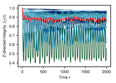
Figure 2: This plot shows the $Z$-directed integrity ${\cal I}_{Z}(t)$ as a function of time for 15 random samples (blue/green shades) and their average (red). The Hamiltonian parameters in this plot are $J=0.075$ and $\Delta=1.0$. The system is of size $N=14$ and we simulated the time evolution until $t=2000$ using step sizes of $\Delta t=0.1$.

Though this average looks well-behaved, the obtained traces show a wide variety of behaviour from one realization to the next. It is useful to split the traces into two groups: those which decreases exponentially with gentle fluctuations, and those which oscillate wildly within an exponentially decaying envelope. The former of these should dominate any average, and so we expect that our disorder-averaged quantities should softly decay, a finding consistent with previous results in related work Bahri et al. (2015).

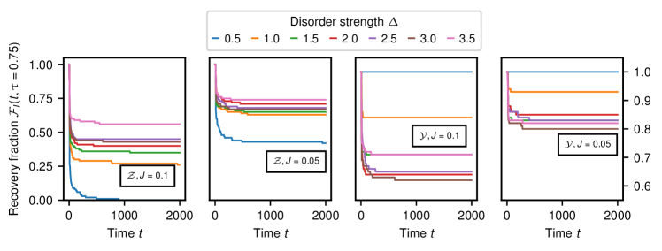
Figure 3: Recovery fractions of directed integrities for a fixed threshold as a function of time. The left two panels show data for two different interaction strengths $J$ for the $Z$-directed integrity $\mathcal{F}_{{\cal I}_{Z}}(t,\tau=0.7)$. The panels on the right show the same interaction strengths $J$ for the $Y$-directed integrity $\mathcal{F}_{I_{Y}}(t,\tau=0.7)$. Note the different scale of the y-axes. Colours encode the disorder strength $\Delta$. The system is of size $N=14$ and we simulated the time evolution until $t=2000$ using step sizes of $\Delta t=0.1$.

While this would usually be the end of a story featuring disorder, the appearance of rapidly fluctuating traces is very concerning. Since a low value in the integrity and coherent information both indicate the formation of entanglement, we can only conclude that the edge state is oscillating between states of high and low bulk entanglement. This scenario constitutes a fiendish obstacle for any experimental implementation. Even if one could in principle decode the stored data by picking a moment of low entanglement, the experimenter would need detailed knowledge about the system dynamics to do so reliably. One might hope that these wild fluctuations are limited to this single integrity plot, indicating a pathology with limited scope. But, as we shall see, they appear in a sizeable fraction of disorder realizations and so are intrinsic to the dynamics of this system.

Given the extreme variation between disorder realizations, we find ourselves in a circumstance where disorder averaging would impede our ability to determine the suitability of this system to act as a quantum memory. Instead, we will define a phenomenological quantity appropriate for the given problem, which we call the recovery fraction

$$\mathcal{F}_{A}(t,\tau):=\frac{N_{\text{rec}}}{N_{\text{tot}}}\,,$$ (19)

where $N_{\text{rec}}$ is defined as the number of instances for which the measured quantity $A$ is larger than $\tau$, i.e. $|\{A(t)|A(t^{\prime})>\tau\quad\forall t^{\prime}\leq t\}|$. The coefficient $\tau$ captures a minimum threshold that a hypothetical experimenter would need in order to recover the encoded information. In the limit of infinite sample size, the recovery fraction converges to a probability. This recovery probability gives the relative proportion of systems that reliably, meaning for all times smaller than $t$, stay above the recovery threshold $\tau$.

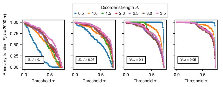
Figure 4: Final recovery fraction of directed integrities at $t=2000$ as a function of the threshold $\tau$. The panels on the left show data for two different interaction strengths $J$ for the $Z$-directed integrity $\mathcal{F}_{{\cal I}_{Z}}(t=2000,\tau)$. The panels on the right show the same interaction strengths $J$ for the $Y$-directed integrity $\mathcal{F}_{I_{Y}}(t=2000,\tau)$. Colours encode the disorder strength $\Delta$. The system is of size $N=14$.

IV.1 Directed integrities

We first investigate the directed integrities ${\cal I}_{X}(t),I_{Y}(t),{\cal I}_{Z}(t)$, which quantify how well the two initially orthogonal states in the $X,Y,$ or $Z$ logical basis remain so. Each of these gives an upper bound to the true integrity, but there are significant differences between these bases which require comment.

As described above, we will look at the recovery fraction to identify which realizations would be unusable due to rapid oscillatory behaviour. Fig. 3 shows the time evolution of the recovery fraction for each directed integrity. The left panels show the recovery fraction for the $Z$-directed integrity $\mathcal{F}_{{\cal I}_{Z}}(t,\tau=0.7)$ for interaction strengths $J\in\{0.1,0.05\}$. Colours encode the different disorder strengths. For any combination of Hamiltonian parameters, we find a steep initial drop of the recovery probability followed by a long plateau. When tuning the strengths of the interactions and disorder, we find that decreasing interactions and increasing disorder increases the apparent saturation value of the recovery probability. This is plausibly explained by the sharper localization behaviour in such conditions, a mechanism that conceivably improves the storage of classical information. The sharp initial drop-off is both intriguing and highly disturbing, as it implies that even for relatively weak interaction strengths (e. g. $J=0.05$), a huge fraction of disorder realizations fall below threshold immediately. The loss of 25% to 50% of these shows that, while the overall decay profile may be exponential, the fine structure of the evolution would preclude us from saying that the information is protected in any practical sense. We would like to point out that the $X$-directed integrity shows the same qualitative behaviour and thus is not displayed separately here.

When analysing the recovery fraction for the $Y$-directed integrity $\mathcal{F}_{I_{Y}}(t,\tau=0.7)$ shown in the two panels on the right, we find a sizeable quantitative increase of the recovery fraction accompanied by a similar qualitative effect of interactions, namely the recovery probability decreases with interaction strength. However, its disorder dependence differs significantly from the ${\cal I}_{Z}(t)$ case. Here, increasing the disorder strength decreases the integrity of the $Y$-basis. Moreover, the recovery fraction is the lowest when the disorder strength is large enough to cancel the mean bulk gap ($\Delta\geq 2$). While initially shocking, the large quantitative and qualitative difference between bases actually mirrors results from previous numerical studies performed by some of the authors Goihl et al. (2019), where the perturbed edge zero mode operators showed a similar disorder and interaction dependence.

While the time dependence of $\mathcal{F}_{I}$ reveals curious behaviour, in practice, an experimenter will be interested in how well the bit can be recovered after time evolution. It is thus instructive to consider the final value of our simulation at $t=2000$ and plot this value as a function of the threshold $\tau$, ensuring that we have not artificially depressed the recovery fraction by choosing an overly optimistic threshold. The resulting plots are shown in Fig. 4. Again, the colour encodes disorder and the two panels on the left show two interaction strengths $J\in\{0.1,0.05\}$ for the final recovery fraction of the $Z$-directed integrity $\mathcal{F}_{{\cal I}_{Z}}(t=2000,\tau)$. Here, we find that the recovery fraction starts at one and smoothly goes to zero when the threshold reaches one. Again, the interaction plays a crucial role here, depressing the recovery fraction uniformly as it increases. The disorder blunts this effect as before, but the effect saturates when it is of the order of the mean bulk gap. When turning to the final recovery fraction of the $Y$-directed integrity $\mathcal{F}_{I_{Y}}(t=2000,\tau)$ shown in the two panels on the right, we again see an extreme sensitivity to the disorder strength, with a final recovery fraction which is almost identically 1 for all but the most aggressive values of $\tau$ while disorder is very low ($<0.5$), with an immediate drop-off for higher disorder strengths. What becomes more apparent is disorder’s homogenization of the bases, improving the integrity of the $X$ and $Z$ encodings while simultaneously degrading the $Y$ encoding so that the final recovery fractions are similar.

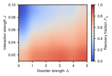
Figure 5: In this heat map, we show the disorder and interaction dependence of the final recovery fraction $\mathcal{F}_{{\cal I}_{Z}}(t=2000,\tau=0.7)$ for a fixed threshold for the $Z$-directed integrity.

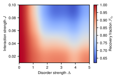
Figure 6: In this heat map, we show the disorder and interaction dependence of the final recovery fraction $\mathcal{F}_{I_{Y}}(t=2000,\tau=0.7)$ for a fixed threshold for the $Y$-directed integrity.

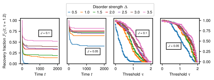
Figure 7: This plot shows data for the coherent information for interaction strengths $J\in\{0.1,0.05\}$. Panels on the left show the time evolution of the recovery fraction of the coherent information $\mathcal{F}_{C}(t,\tau=1.2)$. Colours encode the disorder strength $\Delta$. The system is of size $N=14$. Simulations run up to $2000$ tunnelling times with a step size of $\Delta t=0.1$. Panels on the right show the final recovery fraction of the coherent information $\mathcal{F}_{C}(t=2000,\tau)$ as a function of the threshold $\tau$ for the same interaction and disorder strengths.

These results are nicely summarised in Fig. 5 and  6, heat maps of $\mathcal{F}_{{\cal I}_{Z}}(t,\tau=0.7)$ and $\mathcal{F}_{I_{Y}}(t,\tau=0.7)$ respectively. Here we can clearly see the monotonic improvement of the $Z$-directed integrity with increasing disorder and decreasing interaction strength, while the $Y$-directed integrity shows a clear dip as $\Delta$ approaches 2. We do see a resurgence in both plots when $\Delta$ moves beyond 4, but this corresponds to the disorder scale becoming the dominant energy scale in the problem, playing a similar role to the mean gap in the original problem.

Taken together, the directed integrities paint a curious picture. Classical bits encoded using any basis will be susceptible to degradation from interactions. Bizarrely, our ability to attenuate this with disorder depends more on the chosen edge basis than the interaction strength, with the $Y$-basis being clearly superior for weak disorder. We would like to stress again, that considering single directed integrities only allows conclusions about the classical information storage. The actual integrity is the minimum of all possible encodings, and is thus upper bounded by the worst of our directed integrity results, e.g. the $Z$-directed integrity. Since this is improved by introducing disorder, this suggests that disorder does in fact help its ability to store quantum information, albeit at the cost of reducing its classical information storage capabilities, which are captured by the $Y$-directed integrity. To confirm this, we will now calculate the coherent information of the dynamical map.

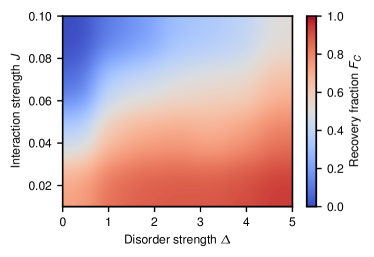
Figure 8: In this heat map, we show the disorder and interaction dependence of the final recovery fraction of the coherent information $\mathcal{F}_{C}(t=2000,\tau=1.2)$.

IV.2 Coherent information

In this part, we carry out the very same analysis as for the directed integrities but now we use the coherent information $C(t)$ which gives a lower bound to the single-shot capacity $Q_{1}(t)$ of our system. $Q_{1}(t)$ quantifies the number of qubits which could be reliably be extracted from our system after our time evolution using some optimal single-shot encoding strategy. The coherent information then corresponds to fixing an encoding strategy, and thus both range from zero to two.

The time dependence of the recovery fraction of the coherent information $\mathcal{F}_{C}(t,\tau=1.2)$ for a fixed threshold and different interaction strengths is shown in the left panels of Fig. 7. The behaviour shown is strikingly similar to the $Z$-directed integrity, showing the same immediate decline in recovery fraction, but now for a quantity which is genuinely quantum. Decreasing the interaction strength and increasing the disorder strength both improve the coherent information monotonically, a feature also shared with the $Z$-directed integrity. These similarities continue in the final recovery probability of the coherent information $\mathcal{F}_{C}(t=2000,\tau)$ as a function of cutoff $\tau$ shown in the panels on the right in Fig. 7, showing that most of the improvement comes from reducing the interaction strength.

If we now again consider the final recovery probability of the coherent information $\mathcal{F}_{C}(t=2000,\tau=1.2)$ with fixed threshold as a function of disorder and interaction strength shown in Fig. 8, we again see that high disorder and low interaction lead to the highest final recovery fraction of the coherent information. The figure looks very similar to what we have obtained for the $Z$-directed integrities, confirming that the ability of these to store information is the limiting factor in edge’s ability to preserve quantum information reliably.

V Conclusions

Using edge modes of topologically protected systems is a promising avenue for quantum information tasks. It is, however, largely unclear how stable information encoded into these systems will actually be when the system is perturbed away from its solvable point by spurious interactions and disorder, both of which are omnipresent in realistic experimental realizations. Here, we present numerical results for the dynamical recoverability of information – both classical and quantum – encoded into the edge mode subspace of an $XZX$ cluster Hamiltonian with both tunable many-body interactions and disorder as a perturbation. We reconstruct the edge state density matrix to obtain the channel which represents the time evolution. With these data, we are in position to calculate measures of classical information, namely directed integrities; and quantum information, namely the coherent information.

Studying the directed integrities, we find that not only disorder strength and interaction strength change the amount of recoverable information, but also that the specific encoding direction plays a crucial role in determining the coherence of the encoded bits. The best encoding is found to be in the $Y$ basis of the unperturbed Hamiltonian, yielding very stable bits for a large range of interaction strengths and low disorder. The narrative of disorder aiding the encoding is wrong for this setting. It holds, however, for an encoding in the $Z$ or $X$ bases, where the detrimental effect of interaction strength can be counteracted by introducing disorder.

For quantum information, we recover and provide further substance to the narrative that disorder increases the ability of the system to store quantum information. Interactions decrease the quality of the memory in a similar way to the classical encoding in $Z$ or $X$ direction.

To distinguish well- and ill-behaved disorder realizations, we set a minimum performance threshold and evaluated the fraction of runs which stayed above it over the course of the evolution. Quite surprisingly, this fraction failed to decay smoothly over time, as one would expect if there was gradual decoherence of the edge states. Instead, the recover fraction dropped precipitously, indicating that a large fraction of disorder realizations describe systems that would be worthless for information storage purposes. Furthermore, these may not have an appreciable effect on disorder averages, as they are rapidly oscillatory instead of simply dropping to zero immediately. It seems fair to say that the interplay of disorder, interactions and SPT order is less understood than previously anticipated. Our findings are compatible with those in Ref. Goihl et al. (2019), where a similarly multi-faceted picture for the edge mode support was found using a completely different method. These results demand more foundational work possibly including an extension of perturbation theory to systems with topologically protected degeneracies.

Our work covers information loss due to unitary dynamics under perturbed Hamiltonians, but real world experiments are also coupled to the outside world leading to further decoherence. Since localization effects are also expected to be diminished in the presence of dissipation van Nieuwenburg et al. (2017); Lüschen et al. (2017), the amount of information protection induced by disorder seems questionable. Given that open system dynamics are also capable of corrupting topological data directly, even without the presence of many-body interactions Budich et al. (2012); Rainis and Loss (2012); Mazza et al. (2013), investigating the circumstances where disorder, interactions, and a particle reservoir are all present is likely to yield fascinating results.

VI CO₂-emission table

Here, we summarize the climate expenses of the simulations presented in this work.

Numerical simulations
Total Kernel Hours [$\mathrm{h}$]	308000
Thermal Design Power per Kernel [$\mathrm{W}$]	5.75
Total Energy Consumption of Simulations [$\mathrm{kWh}$]	1771
Average Emission of CO2 in Germany [$\mathrm{kg/kWh}$]	0.56
Total CO2-Emission from Numerical Simulations [$\mathrm{kg}$]	992
Were the Emissions Offset?	Yes
Transportation
Total CO2-Emission from Transportation [$\mathrm{kg}$]	0
Were the Emissions Offset?	Yes
Total CO2-Emission [$\mathrm{kg}$]	992

Figure 9: Estimated climate footprint of the computations presented in this paper. Prototyping is not included in these calculations. Estimations have been calculated using the examples of Scientific CO₂nduct Goihl and Sweke and are correct to the best of our knowledge.

VII Acknowledgements

We would like to thank Ingo Roth for discussions on optimization schemes. NW acknowledges funding support from the European Unions Horizon 2020 research and innovation programme under the Marie Sklodowska-Curie grant agreement No.750905. This work has been supported by the ERC (TAQ), the DFG (CRC 183, FOR 2724, EI 519/7-1), and the Templeton Foundation. This work has also received funding from the European Union’s Horizon2020 research and innovation programme under grant agreement No 817482 (PASQuanS).

References

- Gross and Bloch (2017) C. Gross and I. Bloch, Science 357, 995 (2017).
- Blatt and Roos (2012) R. Blatt and C. F. Roos, Nature Phys. 8, 277 (2012).
- Aspuru-Guzik and Walther (2012) A. Aspuru-Guzik and P. Walther, Nature Phys. 8, 285 (2012).
- Eisert et al. (2015) J. Eisert, M. Friesdorf, and C. Gogolin, Nature Phys. 11, 124 (2015).
- Dennis et al. (2002) E. Dennis, A. Kitaev, A. Landahl, and J. Preskill, J. Math. Phys. 43, 4452 (2002).
- Kitaev (2003) A. Y. Kitaev, Ann. Phys. 303, 2 (2003).
- Kitaev and Preskill (2006) A. Kitaev and J. Preskill, Phys. Rev. Lett. 96, 110404 (2006).
- Haldane (1983) F. D. M. Haldane, Phys. Rev. Lett. 50, 1153 (1983).
- Kitaev (2001) A. Y. Kitaev, Physics-Uspekhi 44, 131 (2001).
- Verresen et al. (2017) R. Verresen, R. Moessner, and F. Pollmann, Phys. Rev. B 96, 165124 (2017).
- Wen (2013) X.-G. Wen, Phys. Rev. D 88, 045013 (2013).
- Chen et al. (2013) X. Chen, Z.-C. Gu, Z.-X. Liu, and X.-G. Wen, Phys. Rev. B 87, 155114 (2013).
- Miller and Miyake (2015) J. Miller and A. Miyake, Phys. Rev. Lett. 114, 120506 (2015).
- Stephen et al. (2017) D. T. Stephen, D.-S. Wang, A. Prakash, T.-C. Wei, and R. Raussendorf, Phys. Rev. Lett. 119, 010504 (2017).
- Raussendorf et al. (2017) R. Raussendorf, D.-S. Wang, A. Prakash, T.-C. Wei, and D. T. Stephen, Phys. Rev. A 96, 012302 (2017).
- Anderson (1958) P. W. Anderson, Phys. Rev. 109, 1492 (1958).
- Abanin et al. (2019) D. Abanin, E. Altman, I. Bloch, and M. Serbyn, Rev. Mod. Phys. 91, 021001 (2019).
- Gogolin and Eisert (2016) C. Gogolin and J. Eisert, Rep. Prog. Phys. 79, 56001 (2016).
- Huse et al. (2013) D. A. Huse, R. Nandkishore, V. Oganesyan, A. Pal, and S. L. Sondhi, Phys. Rev. B 88, 014206 (2013).
- Chandran et al. (2014) A. Chandran, V. Khemani, C. R. Laumann, and S. L. Sondhi, Phys. Rev. B 89, 144201 (2014).
- Kjäll et al. (2014) J. A. Kjäll, J. H. Bardarson, and F. Pollmann, Phys. Rev. Lett. 113, 107204 (2014).
- Bahri et al. (2015) Y. Bahri, R. Vosk, E. Altman, and A. Vishwanath, Nature Comm. 6, 7341 (2015).
- Goihl et al. (2019) M. Goihl, C. Krumnow, M. Gluza, J. Eisert, and N. Tarantino, SciPost Phys. 6, 72 (2019).
- Goihl et al. (2018) M. Goihl, M. Gluza, C. Krumnow, and J. Eisert, Phys. Rev. B 97, 134202 (2018).
- Briegel et al. (1998) H.-J. Briegel, W. Dür, J. I. Cirac, and P. Zoller, Phys. Rev. Lett. 81, 5932 (1998).
- Muralidharan et al. (2016) S. Muralidharan, L. Li, J. Kim, N. Lütkenhaus, M. D. Lukin, and L. Jiang, Scient. Rep. 6, 20463 (2016).
- Chen et al. (2018) C. Chen, F. Burnell, and A. Chandran, Phys. Rev. Lett. 121, 085701 (2018).
- Affleck et al. (1988) I. Affleck, T. Kennedy, E. H. Lieb, and H. Tasaki, Commun. Math. Phys. 115, 477 (1988).
- Affleck et al. (1987) I. Affleck, T. Kennedy, E. H. Lieb, and H. Tasaki, Phys. Rev. Lett. 59, 799 (1987).
- Serbyn et al. (2013) M. Serbyn, Z. Papić, and D. A. Abanin, Phys. Rev. Lett. 111, 127201 (2013).
- Huse et al. (2014) D. A. Huse, R. Nandkishore, and V. Oganesyan, Phys. Rev. B 90, 174202 (2014).
- Schreiber et al. (2015) M. Schreiber, S. S. Hodgman, P. Bordia, H. P. Lüschen, M. H. Fischer, R. Vosk, E. Altman, U. Schneider, and I. Bloch, Science 349, 842 (2015).
- Choi et al. (2016) J.-Y. Choi, S. Hild, J. Zeiher, P. Schauß, A. Rubio-Abadal, T. Yefsah, V. Khemani, D. A. Huse, I. Bloch, and C. Gross, Science 352, 1547 (2016).
- Acin et al. (2018) A. Acin, I. Bloch, H. Buhrman, T. Calarco, C. Eichler, J. Eisert, D. Esteve, N. Gisin, S. J. Glaser, F. Jelezko, S. Kuhr, M. Lewenstein, M. F. Riedel, P. O. Schmidt, R. Thew, A. Wallraff, I. Walmsley, and F. K. Wilhelm, New J. Phys. 20, 080201 (2018).
- Xu et al. (2018) X. Xu, N. de Beaudrap, J. O’Gorman, and S. C. Benjamin, New J. Phys. 20, 023009 (2018).
- Svore et al. (2005) K. M. Svore, A. W. Cross, I. L. Chuang, and A. V. Aho, Quant. Inf. Comp. 6, 193 (2005).
- Cross et al. (2009) A. W. Cross, D. P. Divincenzo, and B. M. Terhal, Quant. Inf. Comp. 9, 0541 (2009).
- Wilde (2013) M. M. Wilde, Quantum Information Theory (Cambridge University Press, Cambridge, 2013).
- Nielsen and Chuang (2000) M. A. Nielsen and I. L. Chuang, Quantum Computation and Quantum Information (Cambridge University Press, 2000).
- Hradil (1997) Z. Hradil, Phys. Rev. A 55, 1561 (1997).
- White et al. (1999) A. G. White, D. F. V. James, P. H. Eberhard, and P. G. Kwiat, Phys. Rev. Lett. 83, 3103 (1999).
- Roos et al. (2004) C. F. Roos, G. P. T. Lancaster, M. Riebe, H. Häffner, W. Hänsel, S. Gulde, C. Becher, J. Eschner, F. Schmidt-Kaler, and R. Blatt, Phys. Rev. Lett. 92, 220402 (2004).
- Steffen et al. (2006) M. Steffen, M. Ansmann, R. C. Bialczak, N. Katz, E. Lucero, R. McDermott, M. Neeley, E. M. Weig, A. N. Cleland, and J. M. Martinis, Science 313, 1423 (2006).
- Lvovsky and Raymer (2009) A. Lvovsky and M. Raymer, Rev. Mod. Phys. 81, 299 (2009).
- van Nieuwenburg et al. (2017) E. van Nieuwenburg, J. Y. Malo, A. Daley, and M. Fischer, Quant. Sc. Tech. 3, 01LT02 (2017).
- Lüschen et al. (2017) H. P. Lüschen, P. Bordia, S. S. Hodgman, M. Schreiber, S. Sarkar, A. J. Daley, M. H. Fischer, E. Altman, I. Bloch, and U. Schneider, Phys. Rev. X 7, 011034 (2017).
- Budich et al. (2012) J. C. Budich, S. Walter, and B. Trauzettel, Phys. Rev. B 85, 121405 (2012).
- Rainis and Loss (2012) D. Rainis and D. Loss, Phys. Rev. B 85, 174533 (2012).
- Mazza et al. (2013) L. Mazza, M. Rizzi, M. D. Lukin, and J. I. Cirac, Phys. Rev. B 88, 205142 (2013), arXiv:1212.4778 .
- (50) M. Goihl and R. Sweke, in preparation .