Gibbs sampling for game-theoretic modeling of private network upgrades with distributed generation

Abstract

Renewable energy is increasingly being curtailed, due to oversupply or network constraints. Curtailment can be partially avoided by smart grid management, but the long term solution is network reinforcement. Network upgrades, however, can be costly, so recent interest has focused on incentivising private investors to participate in network investments. In this paper, we study settings where a private renewable investor constructs a power line, but also provides access to other generators that pay a transmission fee. The decisions on optimal (and interdependent) renewable capacities built by investors, affect the resulting curtailment and profitability of projects, and can be formulated as a Stackelberg game. Optimal capacities rely jointly on stochastic variables, such as the renewable resource at project location. In this paper, we show how Markov chain Monte Carlo (MCMC) and Gibbs sampling techniques, can be used to generate observations from historic resource data and simulate multiple future scenarios. Finally, we validate and apply our game-theoretic formulation of the investment decision, to a real network upgrade problem in the UK.

I Introduction

Renewable energy sources (RES) play a key role in the climate change mitigation agenda. RES are variable, depend on weather patterns and are difficult to predict, hence raise technical challenges regarding network management. Moreover, grid infrastructure is often inadequate to support RES development, especially in the area of distribution networks. For instance, often RES projects are clustered in remote areas of the grid, where planning approval may be favourable and renewable resources abundant. Typically, in the UK, such areas are windy islands with constrained connections to the main grid. In these areas, technical limitations and imbalance of renewable supply to demand, often result in RES curtailment, i.e. the energy that could have been generated is wasted as the system cannot absorb it or transfer it where required.  Curtailment can affect implementation of future RES projects, result in lost revenues and instigate socio-economic challenges, especially when local community-owned projects are involved.

Typically, RES generators are granted firm connections to the grid and receive compensation for incurred curtailment, the cost of which is eventually borne by all system users. However in several occasions, RES generators are offered interruptible, non-firm connections, as an alternative to expensive or time consuming reinforcements. The so-called flexible commercial arrangements are increasingly offered by network operators, as an alternative, and are creating a shift in network access rules. A detailed review on flexible commercial arrangements can be found in [1, 2]. As shown in [3], arrangements that are fair and equally share curtailment and access among generators, can maximise the generation capacity built at a certain location and minimise discouragement for future investors.

Solutions to reduce curtailment include demand side management, energy storage or smart grid techniques such as Dynamic Line Rating (DLR) or real-time monitoring of the thermal state of the lines [4] and Active Network Management (ANM), i.e., the automatic control of the power system by control devices and data that allow real time operation and optimal power flows [5]. The long term solution, however, is network upgrade. Anaya & Pollit (2015) compared smart interruptible connections to traditional grid reinforcements in [5].  It is estimated that, by 2030 in the US alone, up to $2 trillion will be required for network upgrades [6]. As grid expansion is expensive, it is desirable to provide incentives to private parties for taking part in such investments.  Private network upgrades have been studied in several works [7, 8].  However, they raise the question for system operators of defining the framework within which these private lines are incentivised, built and accessed by competing generators.

New private lines constructed, often follow a ‘single access’ principle, i.e. lines for sole-use that suffice only to accommodate the RES capacity of each project. However, as shown in [3], it is possible for system operators to encourage RES generators to install larger capacity lines under a ‘common access’ principle, i.e. a private investor is licensed to build a line only if it grants access to smaller generators, which are subject to transmission charges. In these settings, curtailment and line access rules can play a significant role in the resulting grid expansion. Crucially, this leads to a leader-follower or a Stackelberg game between the line investor and local generators respectively. Stackelberg games in network upgrades and RES settings have been presented in [9, 10]. Our previous work was one of the first to introduce Stackelberg game formulations in settings that combine network upgrades, curtailment and line access rules,  however the model presented in [3] did not take into account stochastic generation and demand required for equilibrium estimation. Subsequent work [11] improved by utilising real data, however, followed a one-shot, single scenario approach. We build on this work by developing a principled framework, based on game-theoretic and state-of-the-art sampling techniques, i.e. Markov chain Monte Carlo (MCMC). Several authors used MCMC for modelling of wind speeds or wind power outputs [12, 13].  Our framework allows modelling multiple renewable investment scenarios that reduce the uncertainty of future generation and demand.  In more detail, the main contributions of the work are:

• We develop a new methodology that generates observations from renewable resource data. While historic data, such as wind speeds may be available, they might have considerable gaps and joint distributions cannot be expressed in simple, closed-form equations. For this reason we develop a MCMC methodology (Gibbs sampling) that can draw samples from available data and run multiple scenarios of potential futures.

• We establish a methodology that can determine optimal generation capacity investments through use of real demand and wind speed data. This work is one of the first to combine Stackelberg equilibria to a large-scale realistic game with MCMC techniques. Our model designates players’ actions, depending on RES output correlation and expected curtailment, and studies the cost parameters effects on the equilibrium of the game.

• Previous work has been extended to account for varying demand data instead of an average approach followed in both [3, 11]. The model is applied and validated in a real network upgrade problem in the UK.

Section II of the paper presents the theoretical formulation of the game, Section III introduces Gibbs sampling, Section IV demonstrates the methodology based on a real-world case study, Section V shows the results and Section VI concludes.

II Stackelberg game model description

Consider a simplified two-node network: location A is a net consumer (area of high demand) and location B is a net producer (area of high wind resource). Moreover, consider two players: a line investor, who can be merchant-type or a utility company and is building i) the AB interconnection and ii) $\textstyle{P_{N_{1}}}$ renewable capacity at B, and a local player representing all local RES generators located at B, and who builds renewable capacity equal to $\textstyle{P_{N_{2}}}$. This second player can be thought of as investors from the local community, who do not have the technical/financial capacity to build a line, but may have access to cheaper land, find it easier to get social approval to build turbines etc., hence may have lower costs for RES deployment.

Building the line will elicit a reaction from local investors. Crucially, the line investor has a first mover advantage in building the grid infrastructure, which is expensive, technically challenging, and only few investors (e.g. DNO-approved) have the expertise and regulatory approval to carry it out. From a game-theoretic perspective, this is a bi-level Stackelberg game, between the leader (line investor or first player) and follower (local generators or second player). We assume that players’ actions are driven by profit maximisation criteria. The profit functions of players can be expressed as in [11]:

$$\Pi_{1}=(E_{G_{1}}-E_{C_{1}})p_{G}-E_{G_{1}}c_{G_{1}}+(E_{G_{2}}-E_{C_{2}})p_{T}-C_{T}$$ (1)

$$\Pi_{2}=(E_{G_{2}}-E_{C_{2}})(p_{G}-p_{T})-E_{G_{2}}c_{G_{2}}$$ (2)

In these equations, $\textstyle{E_{G_{i}}}$ represents player’s $i$ expected energy produced over the project lifetime, if no curtailment occurred, while $\textstyle{E_{C_{i}}}$ is the energy lost through curtailment. Line cost is estimated as $\textstyle{C_{T}=I_{T}+M_{T}}$, where $\textstyle{I_{T}}$ is the cost of building the line (or initial investment) and $\textstyle{M_{T}}$ the cost of operation and maintenance. The monetary value of the power line is proportional to the energy flowing from B to A, charged for local generators and ‘common access’ rules with $\textstyle{p_{T}}$ transmission fee per energy unit transported through the line.  Moreover, the cost of expected generation per unit is defined as $\textstyle{c_{G_{i}}=(I_{G,i}+M_{G_{i}})/{E_{G_{i}}}}$, where $\textstyle{I_{G_{i}}}$ is the cost of building the plant and $\textstyle{M_{G_{i}}}$ the operation and maintenance costs. Finally, the energy generated by a RES unit is sold at a constant generation tariff price, equal to $\textstyle{p_{G}}$.

As seen in Eq. (1), the line investor has two streams of revenue, the self-produced energy and the energy produced by local generators and transported through the line. The costs of the line investor relate to installing and operating the RES capacity ($c_{G_{1}}$) and to building the power line ($C_{T}$). Similarly from Eq. (2), the profits of the local generators depend only on the energy produced (generation cost $c_{G_{2}}$) and transmitted through the line at a charge of $p_{T}$.

The research question our model tries to answer is ‘How to determine the optimal generation capacities $P_{N_{i}}$ built by the two players, so that profits are maximised?’  To answer this question, the profit equations, Eq. (1) and Eq. (2), need to be expressed in terms of generation capacities.

Following the analysis presented in [11], expected generation $\textstyle{E_{G_{i}}}$ and curtailment $\textstyle{E_{C_{i}}}$ can be expressed as functions of the players’ generation capacities. If $x_{i}$ is the per unit power generated by $i$ player, then this represents a stochastic variable that depends on the wind speed distribution, and is equal to $x_{i}={P_{G_{i}}}/{P_{N_{i}}}$, where $P_{G_{i}}$ is the actual power output of $i$ generator and $P_{N_{i}}$ its rated capacity. If $\mathbb{E}(P_{G_{i,t}})$ is the expected power generated at time interval $t$, then the total energy generated for duration equal to the project’s lifetime is $\displaystyle{E_{G_{i}}=\sum_{t}x_{i}P_{N_{i}}=\sum_{t}\mathbb{E}(P_{G_{i,t}}),\forall t}$. Similarly, the total energy curtailed is $\displaystyle{E_{C}=\sum_{t}\mathbb{E}(P_{C_{t}}),\forall t}$, where $\displaystyle{\mathbb{E}(P_{C_{t}})}$ is the expected power curtailed at time step $t$.

The resulting curtailment depends on wind resources at location B and demand at A, denoted as $P_{D,t}$. Curtailment events happen when $x_{1}P_{N_{1}}+x_{2}P_{N_{2}}-P_{D,t}>0$. Players’ generating plants are located at neighbouring locations at B, therefore experience correlated wind speeds. The stochastic variables $x_{1}$ and $x_{2}$, follow a joint probability distribution function $f(x_{1},x_{2})$ and expected curtailment at time interval $t$ can be expressed as (detailed analysis shown in [11]):

$$\mathbb{E}({P_{C,t}})= \int_{0}^{1}\int_{\frac{P_{D,t}-x_{1}P_{N_{1}}}{P_{N_{2}}}}^{1}(x_{1}P_{N_{1}}+x_{2}P_{N_{2}})f(x_{1},x_{2})dx_{2}dx_{1}$$ (3)

$$-P_{D,t}\int_{0}^{1}\int_{\frac{P_{D,t}-x_{1}P_{N_{1}}}{P_{N_{2}}}}^{1}f(x_{1},x_{2})dx_{2}dx_{1}$$

Crucially, Eq. (3) shows that curtailment depends on both players’ strategies i.e. the generation capacities built. Curtailment expressions for each player under a ‘common access’ regime can be reasonably can be approximated by $E_{C_{i}}=\displaystyle{\frac{E_{G_{i}}}{E_{G_{i}}+E_{G_{-i}}}E_{C}}$ . This concludes the expression of profit equations as functions of players’ rated capacities.

Optimal capacities installed are determined in the equilibrium of the game, which is found by backward induction. The line investor or leader assesses and evaluates the second player’s reaction, in order to determine his strategy (i.e. $\textstyle{P_{N_{1}}}$) and influence the equilibrium price. The leader estimates the follower’s best response, given his own capacity $P_{N_{1}}$:

$$P_{N_{2}}^{*}=\operatorname*{arg\,max}_{P_{N_{2}}}{\Pi_{2}(P_{N_{1}},P_{N_{2}}})$$ (4)

Next, the leader estimates which solution from the set of the local generators’ best response $P_{N_{2}}^{*}$ maximises his own profit:

$$P_{N_{1}}^{*}=\operatorname*{arg\,max}_{P_{N_{1}}}\Pi_{1}(P_{N_{1}},P_{N_{2}}^{*})$$ (5)

In other words, the leader moves first by installing their own capacity. In the second level, followers respond to the capacity built, as anticipated by the leader. The equilibrium of the game $(P_{N_{1}}^{*},P_{N_{2}}^{*})$ satisfies both Eq. (4) and Eq. (5) and is given by the notion of the subgame perfect equilibrium.

In practical settings the joint distribution of stochastic renewable resources is often unknown, but historic data may be available. In addition, due to the interdependency in resulting curtailment and multiple parameters a nice closed-form solution of the game cannot be found or expressed analytically. In [11] we presented an empirical algorithm that utilises directly real data and approximates the solution of the game following a one-shot approach. In addition, data may experience important gaps. In this paper we show how we can utilise real data to simulate scenarios that approximate the real distribution with a state-of-the-art MCMC technique.

III Gibbs sampling

Markov chain Monte Carlo (MCMC) is a class of methods for simulation of stochastic processes. Gibbs sampling can be thought of as a particular case of the Metropolis-Hastings algorithm used for MCMC [14]. The Gibbs sampler uses the conditional distributions as proposal distributions with acceptance probability equal to 1 [15] and can be easily implemented in various applications. Using this technique we can generate, from historic data, observations that are dependent. Wind data samples from the project locations form a Markov chain (MC). We can experiment with the length of the chain or sampling size $n$ and we can repeat the process for multiple MCs or number of realisations $N$. In practice, $n$ and $N$ need to be determined in such way that the resulting MC converges to the real distribution, is ergodic and computationally efficient. Ergodicity means that all possible states of the MC can be visited and are independent of the starting state [15]. The methodology applied is described in detail in the next sections with the help of the Kintyre-Hunterston case study.

IV Case study analysis

IV-A Kintyre-Hunterston link

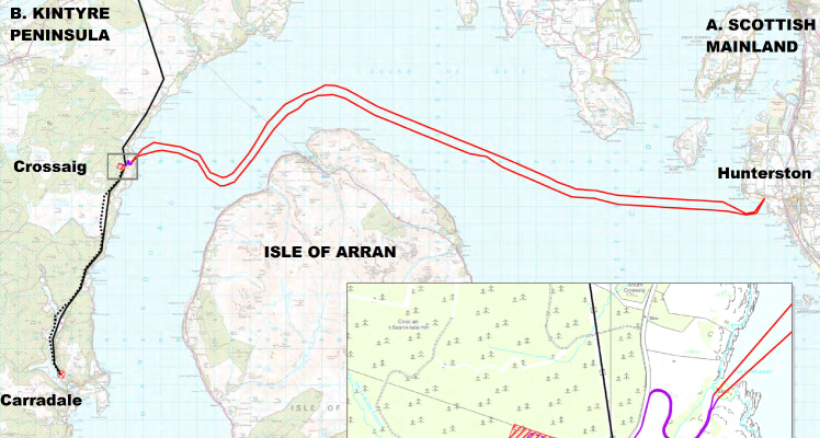
Figure 1: Kintyre-Hunterston project map

The case study analysis is based on a real $\pounds 230\rm{m}$ grid reinforcement project in the UK that links the Kintyre peninsula to the Hunterston substation on the Scottish mainland (see Fig. 1). Kintyre is a region that has attracted vast renewable investment, predominantly wind generation, resulting in the necessity of a newly built power line, which provided space for $150~{}\text{MW}$ of additional renewable capacity.

TABLE I: Results for $N=100$ realisations and an increasing number of observations $n$

Sample size $\bar{w}_{1}$  $\sigma_{\bar{w}_{1}}$ WCI $\bar{w}_{1}$ ME $\bar{w}_{1}$ $\bar{w}_{2}$  $\sigma_{\bar{w}_{2}}$ WCI $\bar{w}_{2}$ ME $\bar{w}_{2}$ $\bar{P}_{D}$  $\sigma_{\bar{P}_{D}}$  WCI $\bar{P}_{D}$ ME $\bar{P}_{D}$ $n=1,000$ $12.1321$ $0.6569$ $0.2607$ $18.91\%$ $12.2297$ $0.6226$ $0.2470$ $17.61\%$ $108.5722$ $0.7859$ $0.3119$ $2.63\%$ $n=5,000$ $12.0853$ $0.2903$ $0.1152$ $6.65\%$ $12.1762$ $0.2797$ $0.1110$ $6.47\%$ $108.6271$ $0.3395$ $0.1348$ $1.49\%$ $n=10,000$ $12.0929$ $0.2262$ $0.0897$ $4.63\%$ $12.1842$ $0.2187$ $0.0869$ $4.36\%$ $108.6000$ $0.2403$ $0.0953$ $1.03\%$ $n=50,000$ $12.1125$ $0.0874$ $0.0347$ $2.02\%$ $12.2028$ $0.0857$ $0.0340$ $1.97\%$ $108.5979$ $0.1033$ $0.0410$ $0.73\%$ $n=100,000$ $12.1155$ $0.0631$ $0.0251$ $1.28\%$ $12.2075$ $0.0602$ $0.0239$ $1.16\%$ $108.5954$ $0.0663$ $0.0263$ $0.70\%$ $n=200,000$ $12.1065$ $0.0441$ $0.0175$ $0.80\%$ $12.1986$ $0.0427$ $0.0169$ $0.76\%$ $108.5915$ $0.0453$ $0.0180$ $0.62\%$ $n=500,000$ $12.1049$ $0.0272$ $0.0108$ $0.68\%$ $12.1968$ $0.0262$ $0.0103$ $0.62\%$ $108.5930$ $0.0288$ $0.0114$ $0.57\%$

TABLE II: Results for $n=5,000$ sampling size and an increasing number of realisations $N$

Realisations $\bar{w}_{1}$  $\sigma_{\bar{w}_{1}}$ WCI $\bar{w}_{1}$ ME $\bar{w}_{1}$ $\bar{w}_{2}$  $\sigma_{\bar{w}_{2}}$ WCI $\bar{w}_{2}$ ME $\bar{w}_{2}$ $\bar{P}_{D}$  $\sigma_{\bar{P}_{D}}$  WCI $\bar{P}_{D}$ ME $\bar{P}_{D}$ $N=100$ $12.0850$ $0.2774$ $0.0840$ $6.64\%$ $12.2017$ $0.2671$ $0.0809$ $6.01\%$ $108.5703$ $0.3037$ $0.0919$ $1.34\%$ $N=170$ $12.1120$ $0.2217$ $0.0879$ $5.35\%$ $12.1812$ $0.2145$ $0.0851$ $5.15\%$ $108.6275$ $0.3279$ $0.1301$ $1.26\%$ $N=500$ $12.0867$ $0.2709$ $0.0476$ $7.22\%$ $12.1764$ $0.2618$ $0.0460$ $7.16\%$ $108.5932$ $0.3052$ $0.0536$ $1.47\%$ $N=1,000$ $12.1097$ $0.2764$ $0.0343$ $8.20\%$ $12.2025$ $0.2666$ $0.0331$ $7.57\%$ $108.5949$ $0.3198$ $0.0397$ $1.47\%$ $N=5,000$ $12.1044$ $0.2793$ $0.0155$ $9.06\%$ $12.1966$ $0.2717$ $0.0151$ $8.81\%$ $108.5951$ $0.3244$ $0.0180$ $1.58\%$ $N=10,000$ $12.1032$ $0.2754$ $0.0108$ $9.41\%$ $12.1956$ $0.2672$ $0.0105$ $8.60\%$ $108.5917$ $0.3268$ $0.0128$ $1.70\%$ $N=50,000$ $12.1022$ $0.2787$ $0.0049$ $9.87\%$ $12.1943$ $0.2707$ $0.0048$ $9.26\%$ $108.5901$ $0.3241$ $0.0057$ $1.70\%$

Following the analysis described in Section II, we assume that the demand region or Location A is Hunterston and location B is the geographical region covering the Kintyre peninsula. The line investor and local generators install generation capacities at different sub-regions of B. Two weather stations were selected by the UK Met Office database, the station with ID 908 located in the Kintyre peninsula (wind farm of line investor) and with ID 23417 located in Islay (wind farm of local generators), with a distance between them of $44~{}\rm{km}$. These weather stations provide data over a common period of 17 years (1999–2015). Demand data used in simulations are based on real UK National Demand data  in the time period of 2006–2015. UK demand data are normalised to represent a lower local demand. More details on the case study and data processing can be found in [11].

Literature in wind forecasting commonly uses Weibull distributions for the representation of actual wind distributions. However, the joint probability distribution of the wind speed (and of the players’ power outputs), exhibits correlation and in practice is not known. If there are sufficient wind speed measurements for both players locations, then the joint probability distribution can be approximated directly from the available historic data. The method described in the following section can be used to draw observations from available data and simulate different scenarios. The technique can generate large datasets as required for the intended analysis.

IV-B Gibbs sampling applied

Algorithm 1 Gibbs Sampling

1:$w_{1}$,$w_{2}$,$P_{D}$ $\triangleright$ wind speed 1,2, power demand

2:$T$ $\triangleright$ number of samples

3:$\langle w_{1}^{(k)},w_{2}^{(k)},P_{D}^{(k)}\rangle$, $k\in\{1,2,...,k_{max}\}$ $\triangleright$ historic data

4:$F(w_{1},w_{2})$ $\triangleright$ wind distribution from data

5:$G\left(P_{D},\displaystyle{\frac{w_{1}+w_{2}}{2}}\right)$ $\triangleright$ demand cond. distrib. on mean wind

6:$t\leftarrow 1$

7:$\langle w_{1}^{(t)},w_{2}^{(t)},P_{D}^{(t)}\rangle\leftarrow sample(w_{1},w_{2},P_{D})$ $\triangleright$ initialise

8:repeat

9:     $w_{1}^{(t+1)}\leftarrow sample$ $F(w_{1}\mid_{w_{2}^{(t)}})$

10:     $w_{2}^{(t+1)}\leftarrow sample$ $F(w_{2}\mid_{w_{1}^{(t+1)}})$

11:     $P_{D}^{(t+1)}\leftarrow sample$ $G\left(P_{D}\mid_{\textstyle{\frac{w_{1}^{(t+1)}+w_{2}^{(t+1)}}{2}}}\right)$

12:     $t\leftarrow t+1$

13:until $t>T$

14:return $\langle w_{1}^{(t)},w_{2}^{(t)},P_{D}^{(t)}\rangle$, $t\in\{t_{burn},t_{burn}+1,...,T\}$

We apply Gibbs sampling to the joint bivariate distribution of wind speeds at the players’ locations. Players’ wind speeds at each time $t$ form a MC. The methodology is described in Alg. 1. From available historic data, we create a joint distribution table of wind speeds at the players’ locations. For every possible wind speed $w_{1}$ of first player, we record the subset of $w_{2}$ wind speed, and vice versa (Line 4 in Alg. 1). This represents the conditional distributions. In practice,the probabilities for certain combinations of wind speeds can be low (e.g. it is unlikely to have extremely high wind at one location and low wind speed to a proximal location), therefore some subsets can be sparse, either because some of observations represent rare events or due to correlation. We overcome this difficulty by merging sparse bins of rare events and outliers, and ensure ergodicity of the MC. The MC is initialised by randomly selecting a sample from the joint distribution table (Line 7 in Alg. 1). Each iteration step involves replacing the value of one variable by a value selected randomly by the conditional $F(w_{i}\mid_{w_{-}i^{(t)}})$. In addition, demand is randomly selected by the conditional distribution of demand over the average wind speed (Line 11 in Alg. 1). The procedure is cycled through the variables forming $n$ samples of $\langle w_{1}^{(t)},w_{2}^{(t)},P_{D}^{(t)}\rangle$, $t\in\{1,2,...,T=n\}$. To ensure that the MC converges, we run Alg. 1 for several sampling sizes $n$ (small, moderate, large) and repeat the procedure for $N$ realisations. Results are shown in Tables I and II. Columns represent the sample mean, standard deviation of the sample mean, width of the 95% confidence interval (WCI) and maximum error (ME) from mean of historic data, i.e. $\mu_{w_{1}}=12.1029$, $\mu_{w_{1}}=12.1950$ and $\mu_{P_{D}}=108.1830$. As the sampling size increases the sample mean follows a normal distribution and the standard deviation decreases, as expected by the central limit theorem (Table I). We perform the same analysis for an increasing number of realisations that use a different starting point (Table II). We also adopt a burn-in or warm-up period of 20% of samples to make sure that our results are independent off the starting state [15]. The results show that MC converges to the distribution from data and that a large $n$ is required but $N$ can be chosen to be relatively small. For this reason and driven by computational limitations, for the estimation of the Stackelberg equilibrium, we selected $n=50,000$, $N=170$ and burn-in of $10,000$ samples.

IV-C Stackelberg equilibrium estimation

Wind speed data generated by the Gibbs sampler are used to estimate the per unit power output of wind generators. Estimation is based on a generic power curve and a sigmoid function approximation (see Alg. 2 Line 4). Players’ strategies are the capacities they can install. The maximum feasible solution for a single player was set equal to $P_{N_{max}}=500.5~{}\text{MW}$ and the incremental capacity to $step=0.5~{}\text{MW}$. For every possible combination of the rated capacities installed $(P_{N_{1}},P_{N_{2}})$, we estimate the power generated and curtailed for each player on an hourly basis. Next, we estimate the aggregate power generated and curtailed by each player as the summation of $40,000$ data points. The procedure is described in Alg. 2.

Algorithm 2 Generation & Curtailment Estimation

1:$P_{N_{max}}$ $\triangleright$ max rated capacity in search space

2:$P_{N_{i}}\leftarrow[0:step:P_{N_{max}}]$ $\triangleright$ strategy space i=1,2 player

3:$\alpha$, $\beta$ $\triangleright$ power curve sigmoid parameters

4:$P_{G_{i}}^{(t)}\leftarrow\displaystyle{\frac{1}{1+e^{-\alpha(w_{1}^{(t)}-\beta)}}}\cdot P_{N_{i}}$ $\triangleright$ generation i player

5:for all $\textit{P}_{N_{1}}\in\{0,...,P_{Nmax}\}$ do

6:     for all $\textit{P}_{N_{2}}\in\{0,...,P_{Nmax}\}$ do      

7:         $RD\leftarrow P_{D}-(P_{G_{1}}+P_{G_{2}})$ $\triangleright$ residual demand

8:         if $\textit{RD}>0$ then $\triangleright$ no curtailment

9:              $RD\leftarrow 0$          

10:         end

11:         $P_{C_{1}}\leftarrow\displaystyle{\frac{P_{G_{1}}\cdot RD}{P_{G_{1}}+P_{G_{2}}}}$ $\triangleright$ curtailment gen 1

12:         $P_{C_{2}}\leftarrow\displaystyle{\frac{P_{G_{2}}\cdot RD}{P_{G_{1}}+P_{G_{2}}}}$ $\triangleright$ curtailment gen 2      

13:     end

14:end

15:$E_{G_{i}}(P_{N_{i}})\leftarrow\displaystyle{\sum P_{G_{i}}}$ $\triangleright$ total gen i

16:$E_{C_{1}}(P_{N_{1}},P_{N_{2}})\leftarrow\displaystyle{\sum P_{C_{1}}}$ $\triangleright$ total curt 1

17:$E_{C_{2}}(P_{N_{1}},P_{N_{2}})\leftarrow\displaystyle{\sum P_{C_{2}}}$ $\triangleright$ total curt 2

18:return $(E_{G_{1}},E_{G_{2}},E_{C_{1}},E_{C_{2}})$

For several cost parameters $(c_{G_{1}},c_{G_{2}},p_{T})$ and feed-in tariff price $p_{G}$, we estimate the profits as defined in Eq. (1) and Eq. (2). For every possible $P_{N_{1}}$, we find the capacity $P_{N_{2}}^{*}$ that maximises the follower’s profits $\Pi_{2}^{*}$ (follower’s best response). From this set of solutions, the leader selects the one that maximises its own profit i.e. $P_{N_{1}}^{*}$ (leader’s best response). The equilibrium of the game is given by the pair $(P_{N_{1}}^{*},P_{N_{2}}^{*})$, which satisfies best response functions as described in Alg. 3.

Algorithm 3 Profit & Stackelberg Equilibria

1:$\textit{p}_{G}$, $\textit{p}_{T}$ $\triangleright$ feed-in tariff, transmission fee

2:$\textit{C}_{T}$ $\triangleright$ cost of line

3:$\textit{c}_{G_{i}}$ $\triangleright$ i player’s generation cost

4:for all $\textit{P}_{N_{1}}\in\{0,...,P_{N_{max}}\}$ do

5:     for all $\textit{P}_{N_{2}}\in\{0,...,P_{N_{max}}\}$ do      

6:         $\Pi_{1}\leftarrow{}(E_{G_{1}}-E_{C_{1}})p_{G}-E_{G_{1}}c_{G_{1}}+$

7:                  $(E_{G_{2}}-E_{C_{2}})p_{T}-C_{T}$

8:         $\Pi_{2}\leftarrow{}(E_{G_{2}}-E_{C_{2}})(p_{G}-p_{T})-E_{G_{2}}c_{G_{2}}$      

9:     end

10:end

11:for all $\textit{P}_{N_{1}}\in\{0,...,P_{N_{max}}\}$ do $\triangleright$ best response gen 2

12:     $\Pi_{2}^{*}\leftarrow\displaystyle{\max_{P_{N_{2}}}{\Pi_{2}(P_{N_{1}},P_{N_{2}}})}$

13:     $P_{N_{2}}^{*}\leftarrow\displaystyle{\operatorname*{arg\,max}_{P_{N_{2}}}{\Pi_{2}(P_{N_{1}},P_{N_{2}}})}$

14:end

15:$\Pi_{1}^{*}\leftarrow\displaystyle{\max_{P_{N_{1}}}{\Pi_{1}(P_{N_{1}},P_{N_{2}}^{*}})}$ $\triangleright$ best response gen 1

16:$P_{N_{1}}^{*}\leftarrow\displaystyle{\operatorname*{arg\,max}_{P_{N_{1}}}{\Pi_{1}(P_{N_{1}},P_{N_{2}}^{*}})}$

17:return $\Pi_{1}^{*},\Pi_{2}^{*},P_{N_{1}}^{*},P_{N_{2}}^{*}$

V Results and discussion

The methodology described in previous sections was followed to run several experiments. Fig. 2 shows the optimal rated capacities built by the players at the equilibrium of the game for $N=170$ realisations. Recall here that every realisation represents a completely different MC generated. The results are satisfactory and show a $10~{}MW$ range in the estimated solutions for optimal rated capacities. Similar results were observed for the optimal profits derived.

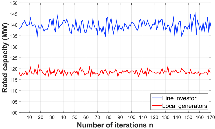
Figure 2: Optimal generation capacities of each player for several realisations ($c_{G_{1}}=0.3p_{G}$, $c_{G_{2}}=0.28p_{G}$, $p_{T}=0.26p_{G}$ and $p_{G}=\pounds 74.3/\text{MWh}$)

Moreover, we study how the equilibrium results depend on varying cost parameters. Fig. 3 shows the dependence on line investor’s cost (first column), local generators’ cost (second column) and the transmission fee (third column). We assume that both players can sell the energy generated for $p_{G}=\pounds 74.3/\text{MWh}$. For each scenario, the key parameter varies, while other parameters remain fixed (Scenario 1: $c_{G_{1}}=0.16\ldots 0.68p_{G}$, $c_{G_{2}}=0.30p_{G}$ and $p_{T}=0.26p_{G}$, Scenario 2: $c_{G_{1}}=0.30p_{G}$, $c_{G_{2}}=0.08\ldots 0.54p_{G}$ and $p_{T}=0.26p_{G}$ and Scenario 3: $c_{G_{1}}=0.26p_{G}$, $c_{G_{2}}=0.20p_{G}$ and $p_{T}=0\ldots 0.80p_{G}$). The results in Fig. 3 show the average equilibrium solution and min-max solutions, found for $N=170$ realisations of the simulation procedure.

$\begin{array}[]{ccc}\includegraphics[width=138.76157pt]{Scen2a}&\includegraphics[width=138.76157pt]{Scen1a}&\includegraphics[width=138.76157pt]{Scen3a}\\ \includegraphics[width=138.76157pt]{Scen2b}&\includegraphics[width=138.76157pt]{Scen1b}&\includegraphics[width=138.76157pt]{Scen3b}\\ \end{array}$

Figure 3: Rows (1) and (2) show generation capacity built and profits at Stackelberg equilibrium, respectively, column (1) shows dependency on generation cost of line investor, (2) on on generation cost of local generators and (3) on transmission fee

In all sets of scenarios, the total capacity installed by all players decreases as the tested parameter value increases. Each player installs less capacity as their generation cost increases, while the other player benefits by increasing their capacity. The cost of local generators has a larger impact on the capacities installed for both players, as shown by comparing the first to the second column. Profits have similar behaviour to the optimal rated capacities, but local generators face the additional cost of transmission charges. If the followers’ generation cost is much lower than the line investor’s (assuming for example that local generators might have access to cheaper land), the line investor needs to charge a high transmission fee to have positive earnings. On the contrary, if the leader’s cost is much lower, the generation capacity will mostly be installed by the line investor, as there is no room for profitable investment from local renewable producers. As shown in Scenario 3, $p_{T}\simeq 0.16p_{G}$ or $\simeq\pounds 12\text{MWh}$ is the minimum value of transmission charges that allows profit for the line investor. Similarly, if the transmission fee is set too high, then it is not profitable for local investors to invest in renewable generation. As $p_{T}$ is set by the system regulator, the methodology can be useful to determine a feasible range of charges that allows both transmission and generation investments to be profitable.

VI Conclusions & Future Work

In this work we show how privately developed network upgrade for DGs can lead to a leader-follower game between the line and local investors. Curtailment and line access rules play a key role in the strategic game, the equilibrium of which determines optimal generation capacities and their profits.  Settings where this model can be applied include numerous locations where demand and generation are not co-located. When real historic data is available, we can use MCMC and Gibbs sampling to simulate multiple future scenarios and reduce the uncertainty of the investment decisions. In the future, we plan to extend the model to multi-location settings and introduce energy storage, which enables using renewable energy to satisfy more of the outstanding demand, and hence reduces curtailment, changing the joint investment game.

References

- [1] A. Laguna Estopier, E. Crosthwaite Eyre, S. Georgiopoulos, and C. Marantes, “FPP low carbon networks: Commercial solutions for active network management,” in CIRED, Stockholm, 2013.
- [2] L. Kane and G. Ault, “A review and analysis of renewable energy curtailment schemes and Principles of Access: Transitioning towards business as usual,” Energy Policy, vol. 72, pp. 67–77, May 2014.
- [3] M. Andoni, V. Robu, and W.-G. Früh, “Game-theoretic modeling of curtailment rules and their effect on transmission line investments,” in IEEE 2012 PES ISGT Europe. IEEE, 2016, pp. 1–6.
- [4] A. Michiorri, R. Currie, P. Taylor, F. Watson, and D. Macleman, “Dynamic line ratings deployment on the Orkney smart grid,” in CIRED, 2011.
- [5] K. L. Anaya and M. G. Pollitt, “Options for allocating and releasing distribution system capacity: Deciding between interruptible connections and firm DG connections,” Applied Energy, vol. 144, pp. 96–105, 2015.
- [6] P. Bronski, J. Creyts, M. Crowdis, S. Doig, J. Glassmire, L. Guccione et al., The economics of load defection: How grid-connected solar-plus-battery systems will compete with traditional electric service-Why it matters, and possible paths forward, 2015.
- [7] L. Maurovich-Horvat, T. K. Boomsma, and A. S. Siddiqui, “Transmission and wind investment in a deregulated electricity industry,” IEEE Trans. on Power Systems, vol. 30, no. 3, pp. 1633–1643, May 2015.
- [8] A. Perrault and C. Boutilier, “Efficient coordinated power distribution on private infrastructure,” in Int. Conference on Autonomous Agents and Multi-Agent Systems. Paris: AAMAS, May 2014, pp. 805–812.
- [9] A. H. van der Weijde and B. F. Hobbs, “The economics of planning electricity transmission to accommodate renewables: Using two-stage optimisation to evaluate flexibility and the cost of disregarding uncertainty,” Energy Economics, vol. 34, no. 6, pp. 2089–2101, Feb. 2012.
- [10] G. E. Asimakopoulou, A. L. Dimeas, and N. D. Hatziargyriou, “Leader-follower strategies for energy management of multi-microgrids,” IEEE Transactions on Smart Grid, vol. 4, no. 4, pp. 1909–1916, Dec. 2013.
- [11] M. Andoni, V. Robu, W.-G. Früh, and D. Flynn, “Game-theoretic modeling of curtailment rules and network investments with distributed generation,” Applied Energy, vol. 201, pp. 174–187, 2017.
- [12] G. Papaefthymiou and B. Klockl, “MCMC for wind power simulation,” IEEE Trans. on Energy Conversion, vol. 23, no. 1, pp. 234–240, 2008.
- [13] T. Wu, X. Ai, W. Lin, J. Wen, and L. Weihua, “Markov chain Monte Carlo method for the modeling of wind power time series,” in 2012 IEEE PES ISGT Asia. IEEE, 2012, pp. 1–6.
- [14] C. Fox and A. Parker, “Convergence in variance of Chebyshev accelerated Gibbs samplers,” SIAM Journal on Scientific Computing, vol. 36, no. 1, pp. A124–A147, 2014.
- [15] C. J. Geyer, “Practical Markov chain Monte Carlo,” Statistical science, pp. 473–483, 1992.