Data ultrametricity and clusterability

Abstract

The increasing needs of clustering massive datasets and the high cost of running clustering algorithms poses difficult problems for users. In this context it is important to determine if a data set is clusterable, that is, it may be partitioned efficiently into well-differentiated groups containing similar objects. We approach data clusterability from an ultrametric-based perspective. A novel approach to determine the ultrametricity of a dataset is proposed via a special type of matrix product, which allows us to evaluate the clusterability of the dataset. Furthermore, we show that by applying our technique to a dissimilarity space will generate the sub-dominant ultrametric of the dissimilarity.

1 Introduction

Clustering is the prototypical unsupervised learning activity which consists in identifying cohesive and well-differentiated groups of records in data. A data set is clusterable if such groups exist; however, due to the variety in data distributions and the inadequate formalization of certain basic notions of clustering, determining data clusterability before applying specific clustering algorithms is a difficult task.

Evaluating data clusterability before the application of clustering algorithms can be very helpful because clustering algorithms are expensive. However, many such evaluations are impractical because they are NP-hard, as shown in [4]. Other notions define data as clusterable when the minimum between-cluster separation is greater than the maximum intra-cluster distance [13], or when each element is closer to all elements in its cluster than to all other data [7].

Several approaches exist in assessing data clusterability. The main hypothesis of [1] is that clusterability can be inferred from an one-dimensional view of pairwise distances between objects. Namely, clusterability is linked to the multimodality of the histogram of inter-object dissimilarities. The basic assumption is that “the presence of multiple modes in the set of pairwise dissimilarities indicates that the original data is clusterable.” Multimodality is evaluated using the Dip and Silverman statistical multimodality tests, an approach that is computationally efficient.

Alternative approaches to data clusterability are linked to the feasibility of producing a clustering; a corollary of this assumption is that “data that are hard to cluster do not have a meaningful clustering structure” [12]. Other approaches to clusterability are identified based on clustering quality measures, and on loss function optimization [4, 9, 3, 8, 7, 11].

We propose a novel approach that relates data clusterability to the extent to which the dissimilarity defined on the data set relate to a special ultrametric defined on the set.

The paper is structured as follows. In Section 2 we introduce dissimilarities and an ultrametrics that play a central role in our definition of clusterability. A special matrix product on matrices with non-negative elements that allow an efficient computation of the subdominant ultrametric is introduced. In Section 3 a measure of clusterability that is based on the iterative properties of the dissimilarity matrix is defined. We provide experimental evidence on the effectiveness of the proposed measure through several experiments on small artificial data sets in Section 4. Finally, we present our conclusions and future plans in Section 5.

2 Dissimilarities, Ultrametrics, and Matrices

A dissimilarity on a set $S$ is a mapping $d:S\times S\longrightarrow\hbox{\bbd R}$ such that

1. $d(x,y)\geqslant 0$ and $d(x,y)=0$ if and only if $x=y$;

2. $d(x,y)=d(y,x)$;

A dissimilarity on $S$ that satisfies the triangular inequality

$$d(x,y)\leqslant d(x,z)+d(z,y)$$

for every $x,y,z\in S$ is a metric. If, instead, the stronger inequality

$$d(x,y)\leqslant\max\{d(x,z),d(z,y)\}$$

is satisfied, $d$ is said to be an ultrametric and the pair $(S,d)$ is an ultrametric space.

A closed sphere in $(S,d)$ is a set $B[x,r]$ defined by

$$B[x,r]=\{y\in S\,\mid\,d(x,y)\leqslant r\}.$$

When $(S,d)$ is an ultrametric space two spheres having the same radius $r$ in $(S,d)$ are either disjoint or coincide [18]. Therefore, the collection of closed spheres of radius $r$ in $S$, ${\cal C}_{r}=\{B[x,r]\,\mid\,r\in S\}$ is a partition of $S$; we refer to this partition as an $r$-spheric clustering of $(S,d)$.

In an ultrametric space $(S,d)$ every triangle is isosceles. Indeed, let $T=(x,y,z)$ be a triplet of points in $S$ and let $d(x,y)$ be the least distance between the points of $T$. Since $d(x,z)\leqslant\max\{d(x,y),d(y,z)\}=d(y,z)$ and $d(y,z)\leqslant\max\{d(y,x),d(x,z)\}=d(x,z)$, it follows that $d(x,z)=d(y,z)$, so $T$ is isosceles; the two longest sides of this triangle are equal.

It is interesting to note that every $r$-spheric clustering in an ultrametric space is a perfect clustering [5]. This means that all of its in-cluster distances are smaller than all of its between-cluster distances. Indeed, if $x,y$ belong to the same cluster $B[u,r]$ then $d(x,y)\leqslant r$. If $x\in B[u,r]$ and $y\in B[v,r]$, where $B[u,r]\cap B[v,r]=\emptyset$, then $d(v,x)>r$, $d(y,v)\leqslant r$ and this implies $d(x,y)=d(x,v)>r$ because the triangle $(x,y,v)$ is isosceles and $d(y,v)$ is not the longest side of this triangle.

Example 2.1.

Let $S=\{x_{i}\,\mid\,1\leqslant i\leqslant 8\}$ and let $(S,d)$ be the ultrametric space, where the ultrametric $d$ is defined by the following table:

$$\begin{array}[]{|c||cccccccc|}\hline\cr d(x_{i},x_{j})&x_{1}&x_{2}&x_{3}&x_{4}&x_{5}&x_{6}&x_{7}&x_{8}\\ \hline\cr x_{1}&0&4&4&10&10&16&16&16\\ x_{2}&4&0&4&10&10&16&16&16\\ x_{3}&4&4&0&10&10&16&16&16\\ x_{4}&10&10&10&0&6&16&16&16\\ x_{5}&10&10&10&6&0&16&16&16\\ x_{6}&16&16&16&16&16&0&4&4\\ x_{7}&16&16&16&16&16&4&0&4\\ x_{8}&16&16&16&16&16&4&4&0\\ \hline\cr\end{array}$$

The closed spheres of this spaces are:

$$B[x_{i},r] = \begin{cases}\{x_{i}\}&\mbox{ for }r<4,\\ \{x_{1},x_{2},x_{3}\}&\mbox{ for }4\leqslant r<10,\\ \{x_{1},x_{2},x_{3},x_{4},x_{5}\}&\mbox{ for }10\leqslant r<16,\\ S&\mbox{ for }r=16,\end{cases}$$

$$\mbox{ for }1\leqslant i\leqslant 3,$$

$$B[x_{i},r] = \begin{cases}\{x_{i}\}&\mbox{ for }r<6,\\ \{x_{4},x_{6}\}&\mbox{ for }6\leqslant r<16,\\ S&\mbox{ for }r=16,\end{cases}$$

$$\mbox{for }4\leqslant i\leqslant 5,$$

$$B[x_{i},r] = \begin{cases}\{x_{i}\}&\mbox{ for }r<4,\\ \{x_{6},x_{7},x_{8}\}&\mbox{ for }4\leqslant r<16,\\ S&\mbox{ for }r=16,\end{cases}$$

$$\mbox{ for }6\leqslant i\leqslant 8.$$

 

Based on the properties of spheric clusterings mentioned above meaningful such clusterings can be produced in linear time in the number of objects. For the ultrametric space mentioned in Example 2.1, the closed spheres of radius $6$ produce the clustering

$$\{x_{1},x_{2},x_{3}\},\{x_{4},x_{5},\},\{x_{6},x_{7},x_{8}\}.$$

If a dissimilarity defined on a data set is close to an ultrametric it is natural to assume that the data set is clusterable. We assess the closeness between a dissimilarity $d$ and a special ultrametric known as the subdominant ultrametric of $d$ using a matrix approach.

Let $S$ be a set. Define a partial order “$\leqslant$” on the set of definite dissimilarities ${\cal D}_{S}$ by $d\leqslant d^{\prime}$ if $d(x,y)\leqslant d^{\prime}(x,y)$ for every $x,y\in S$. It is easy to verify that $({\cal D}_{S},\leqslant)$ is a poset.

The set ${\cal U}_{S}$ of ultrametrics on $S$ is a subset of ${\cal D}_{S}$.

Theorem 2.2.

Let $\{d_{i}\in{\cal U}_{S}\,\mid\,i\in I\}$ be a collection of ultrametrics on the set $S$. Then, the mapping $d:S\times S\longrightarrow\hbox{\bbd R}_{\geqslant 0}$ defined as

$$d(x,y)=\sup\{d_{i}(x,y)\,\mid\,i\in I\}$$

is an ultrametric on $S$.

Proof.

We need to verify only that $d(x,y)$ satisfies the ultrametric inequality $d(x,y)\leqslant\max\{d(x,z),d(z,y)\}$ for $x,y,z\in S$. Since each mapping $d_{i}$ is an ultrametric, for $x,y,z\in S$ we have

$$d_{i}(x,y) \leqslant \max\{d_{i}(x,z),d_{i}(z,y)\}$$

$$\leqslant \max\{d(x,z),d(z,y)\}$$

for every $i\in I$. Therefore,

$$d(x,y) = \sup\{d_{i}(x,y)\,\mid\,i\in I\}$$

$$\leqslant \max\{d(x,z),d(z,y)\},$$

hence $d$ is an ultrametric on $S$. ∎

Theorem 2.3.

Let $d$ be a dissimilarity on a set $S$ and let $U_{d}$ be the set of ultrametrics $U_{d}=\{e\in{\cal U}_{S}\,\mid\,e\leqslant d\}$. The set $U_{d}$ has a largest element in the poset $({\cal U}_{S},\leqslant)$.

Proof.

The set $U_{d}$ is nonempty because the zero dissimilarity $d_{0}$ given by $d_{0}(x,y)=0$ for every $x,y\in S$ is an ultrametric and $d_{0}\leqslant d$.

Since the set $\{e(x,y)\,\mid\,e\in U_{d}\}$ has $d(x,y)$ as an upper bound, it is possible to define the mapping $e_{1}:S^{2}\longrightarrow\hbox{\bbd R}_{\geq 0}$ as $e_{1}(x,y)=\sup\{e(x,y)\,\mid\,e\in U_{d}\}$ for $x,y\in S$. It is clear that $e\leqslant e_{1}$ for every ultrametric $e$. We claim that $e_{1}$ is an ultrametric on $S$.

We prove only that $e_{1}$ satisfies the ultrametric inequality. Suppose that there exist $x,y,z\in S$ such that $e_{1}$ violates the ultrametric inequality; that is,

$$\max\{e_{1}(x,z),e_{1}(z,y)\}<e_{1}(x,y).$$

This is equivalent to

$$\sup\{e(x,y)\,\mid\,e\in U_{d}\}$$

$$> \max\{\sup\{e(x,z)\,\mid\,e\in U_{d}\},$$

$$\sup\{e(z,y)\,\mid\,e\in U_{d}\}\}.$$

Thus, there exists $\hat{e}\in U_{d}$ such that

$$\hat{e}(x,y)>\sup\{e(x,z)\,\mid\,e\in U_{d}\}$$

and

$$\hat{e}(x,y)>\sup\{e(z,y)\,\mid\,e\in U_{d}\}.$$

In particular, $\hat{e}(x,y)>\hat{e}(x,z)$ and $\hat{e}(x,y)>\hat{e}(z,y)$, which contradicts the fact that $\hat{e}$ is an ultrametric. ∎

The ultrametric defined by Theorem 2.3 is known as the maximal subdominant ultrametric for the dissimilarity $d$.

The situation is not symmetric with respect to the infimum of a set of ultrametrics because, in general, the infimum of a set of ultrametrics is not necessarily an ultrametric.

Let ℙ be the set

$$\hbox{\bbd P}=\{x\,\mid\,x\in\hbox{\bbd R},x\geqslant 0\}\cup\{\infty\}.$$

The usual operations defined on ℝ can be extended to ℙ by defining

$$x+\infty=\infty+x=\infty,x\cdot\infty=\infty\cdot x=\infty$$

for $x\geqslant 0$.

Let $\hbox{\bbd P}^{m\times n}$ be the set of $m\times n$ matrices over ℙ. If $A,B\in\hbox{\bbd P}^{m\times n}$ we have $A\leqslant B$ if $a_{ij}\leqslant b_{ij}$ that is, if $a_{ij}\geqslant b_{ij}$ for $1\leqslant i\leqslant m$ and $1\leqslant j\leqslant n$.

If $A\in\hbox{\bbd P}^{m\times n}$ and $B\in\hbox{\bbd P}^{n\times p}$ the matrix product $C=AB\in\hbox{\bbd P}^{m\times p}$ is defined as:

$$c_{ij}=\min\{\max\{a_{ik},b_{kj}\}\,\mid\,1\leqslant k\leqslant n\},$$

for $1\leqslant i\leqslant m$ and $1\leqslant j\leqslant p$.

If $E_{n}\in\hbox{\bbd P}^{n\times n}$ is the matrix defined by

$$(E_{n})_{ij}=\begin{cases}0&\mbox{if }i=j,\\ \infty&\mbox{otherwise},\end{cases}$$

that is the matrix whose main diagonal elements are $0$ and the other elements equal $\infty$, then $AE_{n}=A$ for every $A\in\hbox{\bbd P}^{m\times n}$ and $E_{n}A=A$ for every $A\in\hbox{\bbd P}^{n\times p}$.

The matrix multiplication defined above is associative, hence $\hbox{\bbd P}^{n\times n}$ is a semigroup with the identity $E_{n}$. The powers of $A$ are inductively defined as

$$A^{0} = E_{n},$$

$$A^{n+1} = A^{n}A,$$

for $n\in\hbox{\bbd N}$.

For $A,B\in\hbox{\bbd P}^{m\times n}$ we define $A\leqslant B$ as $a_{ij}\leqslant B_{ij}$ for $1\leqslant i\leqslant m$ and $1\leqslant j\leqslant n$. Note that if $A\in\hbox{\bbd P}^{n\times n}$, then $A\leqslant E_{n}$. It is immediate that for $A,B\in\hbox{\bbd P}^{m\times n}$ and $C\in\hbox{\bbd P}^{n\times p}$, then $A\leqslant B$ implies $AC\leqslant BC$; similarly, if $C\in\hbox{\bbd P}^{p\times m}$ and $CA\leqslant CB$.

Let $L(A)$ be the finite set of elements in ℙ that occur in the matrix $A\in\hbox{\bbd P}^{n\times n}$. Since he entries of any power $A^{n}$ of $A$ are also included in $L(A)$, the sequence $A,A^{2},\ldots,A^{n},\ldots$ is ultimately periodic because it contains a finite number of distinct matrices.

Let $k(A)$ be the least integer $k$ such that $A^{k}=A^{k+d}$ for some $d>0$. The sequence of powers of $A$ has the form

$$\begin{array}[]{l}A,A^{2},\ldots,A^{k(A)-1},A^{k(A)},\ldots,\\ \quad A^{k(A)+d-1},A^{k(A)},\ldots,A^{k(A)+d-1},\ldots,\end{array}$$

where $d$ is the least integer such that $A^{k(A)}=A^{k(A)+d}$. This integer is denoted by $d(A)$.

The set $\{A^{k(A)},\ldots,A^{k(A)+d-1}\}$ is a cyclic group with respect to the multiplication.

If $(S,d)$ is a dissimilarity space, where $S=\{x_{1},\ldots,x_{n}\}$, the matrix of this space is the matrix $A\in\hbox{\bbd P}^{n\times n}$ defined by $a_{ij}=d(x_{i},x_{j})$ for $1\leqslant i,j\leqslant n$. Clearly, $A$ is a symmetric matrix and all its diagonal elements are $0$, that is, $A\leqslant E_{n}$.

If, in addition, we have $a_{ij}\leqslant a_{ik}+a_{kj}$ for $1\leqslant i,j,k\leqslant n$, then $A$ is a metric matrix. If this condition is replaced by the stronger condition $a_{ij}\leqslant\max\{a_{ik}+a_{kj}\}$ for $1\leqslant i,j,k\leqslant n$, then $A$ is ultrametric matrix. Thus, for an ultrametric matrix we have $a_{ij}\leqslant\min\{\max\{a_{ik}+a_{kj}\}\,\mid\,1\leqslant k\leqslant n\}$. This amounts to $A^{2}\leqslant A$.

Theorem 2.4.

If $A\in\hbox{\bbd P}^{n\times n}$ is a dissimilarity matrix there exists $m\in\hbox{\bbd N}$ such that

$$\cdots=A^{m+1}=A^{m}\leqslant\cdots\leqslant A^{2}\leqslant A\leqslant E_{n}$$

and $A^{m}$ is an ultrametric matrix.

Proof.

Since $A\leqslant E_{n}$, the existence of the number $m$ with the property mentioned in the theorem is immediate since there exists only a finite number of $n\times n$ matrices whose elements belong to $L(A)$. Since $A^{m}=A^{2m}$, it follows that $A^{m}$ is an ultrametric matrix. ∎

For a matrix $A\in\hbox{\bbd P}^{n\times n}$ let $m(A)$ be the least number $m$ such that $A^{m}=A^{m+1}$. We refer to $m(A)$ as the stabilization power of the matrix $A$. The matrix $A^{m(A)}$ is denoted by $A^{*}$.

The previous considerations suggest defining the ultrametricity of a matrix $A\in\hbox{\bbd P}^{n\times n}$ with $A\leqslant E_{n}$ as $u(A)=\frac{n}{m(A)}$. Since $m(A)\leqslant n$, it follows that $u(A)\geqslant 1$. If $m(A)=1$, $A$ is ultrametric itself and $u(A)=n$.

Theorem 2.5.

Let $(S,d)$ be a dissimilarity space, where $S=\{x_{1},\ldots,x_{n}\}$ having the dissimilarity matrix $A\in\hbox{\bbd P}^{n\times n}$. If $m$ is the least number such that $A^{m}=A^{m+1}$, then the mapping $\delta:S\times S\longrightarrow\hbox{\bbd P}$ defined by $\delta(x_{i},x_{j})=(A^{m})_{ij}$ is the subdominant ultrametric for the dissimilarity $d$.

Proof.

As we observed, $A^{m}$ is an ultrametric matrix, so $\delta$ is an ultrametric on $S$. Since $A^{m}\leqslant A$, it follows that $d(x_{i},x_{j})\geqslant\delta(x_{i},x_{j})$ for all $x_{i},x_{j}\in S$.

Suppose that $C\in\hbox{\bbd P}^{n\times n}$ is an ultrametric matrix such that $A\leqslant C$, which implies $A^{m}\leqslant C^{m}\leqslant C$. Thus, $A^{m}$ dominates any ultrametric that is dominated by $d$. Consequently, the dissimilarity defined by $A^{m}$ is the subdominant ultrametric for $d$. ∎

The subdominant ultrametric of a dissimilarity is usually studied in the framework of weighted graphs [14].

A weighted graph is a triple $(V,E,w)$, where $V$ is the set of vertices of $G$, $E$ is a set of two-element subsets of $V$ called edges. and $w:E\longrightarrow\hbox{\bbd P}$ is the weight of the edges. If $e\in E$, then $e=\{u,v\}$, where $u,v$ are distinct vertices in $V$. The weight is extended to all 2-elements subsets of $V$ as

$$w(\{v_{i},v_{j}\})=\begin{cases}w(\{v_{i},v_{j}\})&\mbox{if }\{v_{i},v_{j}\}\in E,\\ \infty&\mbox{otherwise}.\end{cases}$$

A path of length $n$ in a weighted graph is a sequence

$$\wp=(v_{0},v_{1},,v_{2},\ldots,v_{n-1},v_{n}),$$

where $\{v_{i},v_{i+1}\}\in E$ for $0\leqslant n\leqslant n-1$.

The set of paths of length $n$ in the graph $G$ is denoted as $\textsf{Paths}^{n}(G)$. The set of paths of length $n$ that join the vertex $v_{i}$ to the vertex $v_{j}$ is denoted by $\textsf{Paths}^{n}_{ij}$. The set of all paths is

$$\textsf{Paths}(G)=\bigcup_{n\geqslant 1}\textsf{Paths}^{n}(G).$$

For a weighted graph $G=(V,E,w)$, the extension of the weight function $w$ to $\textsf{Paths}^{n}(G)$ is the function $M:\textsf{Paths}(G)\longrightarrow\hbox{\bbd P}$ defined as

$$M(\wp)=\max\{w(v_{i-1},v_{i})\,\mid\,1\leqslant i\leqslant n\},$$

where $\wp=(v_{0},v_{1},\ldots,v_{n})$. Thus, if $\wp^{\prime}=\wp e$, we have $M(\wp^{\prime})=\max\{M(\wp),w(e)\}$.

If $G=(V,E,w)$ is a weighted graph, its incidence matrix is the matrix $A_{G}\in\hbox{\bbd P}^{n\times n}$, where $n=|V|$, defined by $(A_{G})_{ij}=w(v_{i},v_{j})$ for $1\leqslant i,j\leqslant n$.

Let $P_{ij}^{(\ell)}$ be the set of paths of length $\ell$ that join the vertex $v_{i}$ to the vertex $v_{j}$. Note that

$$P_{ij}^{(\ell+1)} = \{(v_{i},\ldots,v_{k},v_{j})\,\mid\,$$

$$\wp=(v_{i},\ldots,v_{k})\in P_{ik}^{(\ell)}\mbox{ and }$$

$$v_{j}\mbox{ does not occur in }\wp\}.$$

Define $a_{ij}^{(\ell)}=\min\{M(\wp)\,\mid\,\wp\in P_{ij}^{(\ell)}\}$. The powers of the incidence matrix of the graph are given by

$$a_{ik}^{(\ell+1)} = \min\{M(\wp^{\prime})\,\mid\,\wp^{\prime}\in P_{ik}^{(\ell+1)}\}$$

$$= \min\{\max\{M(\wp),w(e)\}\,\mid\,$$

$$\wp^{\prime}=(v_{i},\ldots,v_{j},v_{k})\mbox{ and }$$

$$\wp\in P_{ij}^{(\ell)},e=(v_{j},v_{k})\in E\}$$

$$= \min_{j}\{\max\{a_{ij}^{\ell},w(e)\}\,\mid\,e=(v_{j},v_{k})\}.$$

Thus, we have

$$(A_{G}^{\ell})_{ij}=\min\{M(\wp)\,\mid\,\wp\in P_{ij}^{\ell}\}$$

for $1\leqslant i,j\leqslant n$.

3 A Measure of Clusterability

We conjecture that a dissimilarity space $(D,d)$ is more clusterable if the dissimilarity is closer to an ultrametric, hence if $m(A_{D})$ is small. Thus, it is natural to define the clusterability of a data set $D$ as the number $\textsf{clust}(D)=\frac{n}{m(A_{D})}$ where $n=|D|$, $A_{D}$ is the dissimilarity matrix of $D$ and $m(A_{D})$ is the stabilization power of $A_{D}$. The lower the stabilization power, the closer $A$ is to an ultrametric matrix, and thus, the higher the clusterability of the data set.

Table 1: All clusterable datasets have values greater than 5 for their clusterability; all non-clusterable datasets have values no larger than $5$.

Dataset	n	Dip	Silv.	$m(A_{D})$	$\textsf{clust}(D)$
iris	150	0.0000	0.0000	14	10.7
swiss	47	0.0000	0.0000	6	7.8
faithful	272	0.0000	0.0000	31	8.7
rivers	141	0.2772	0.0000	22	6.4
trees	31	0.3460	0.3235	7	4.4
USAJudgeRatings	43	0.9938	0.7451	10	4.3
USArrests	50	0.9394	0.1897	15	3.3
attitude	30	0.9040	0.9449	6	5
cars	50	0.6604	0.9931	15	3.3

Our hypothesis is supported by previous results obtained in [1], where the clusterability of 9 databases were statistically examined using the Dip and Silverman tests of unimodality. The approach used in [1] starts with the hypothesis that the presence of multiple modes in the uni-dimensional set of pairwise distances indicates that the original data set is clusterable. Multimodality is assessed using the tests mentioned above. The time required by this evaluation is quadratic in the number of objects.

The first four data sets, iris, swiss, faithful and rivers were deemed to be clusterable; the last five were evaluated as not clusterable. Tests published in [6] have produced low $p$-values for the first four datasets, which is an indication of clusterability. The last five data sets, USArrests, attitude, cars, and trees produce much larger $p$-values, which show a lack of clusterability. Table 1 shows that all data sets deemed clusterable by the unimodality statistical test have values of the clusterability index that exceed $5$.

In our approach clusterability of a data set $D$ is expressed primarily through the “stabilization power” $m(A_{D})$ of the dissimilarity matrix $A_{D}$; in addition, the histogram of the dissimilarity values is less differentiated when the data is not clusterable.

4 Experimental Evidence on Small Artificial Data Sets

Another series of experiments involved a series of small datasets having the same number of points in $\hbox{\bbd R}^{2}$ arranged in lattices. The points have integer coordinates and the distance between points is the Manhattan distance.

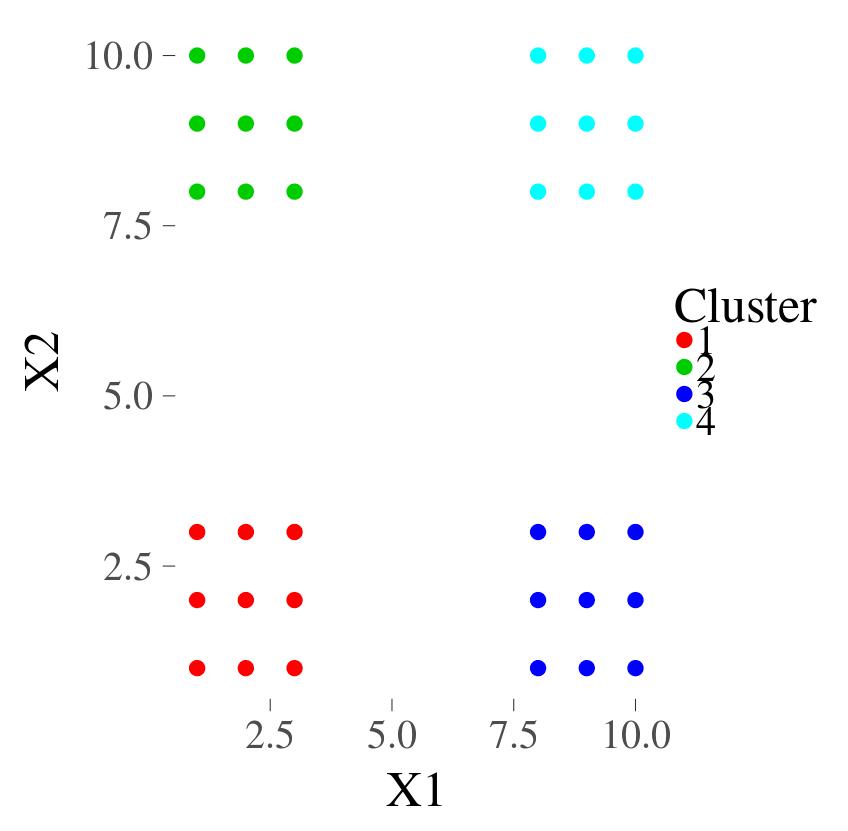
Original dataset
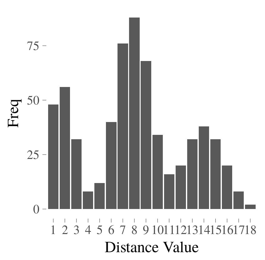
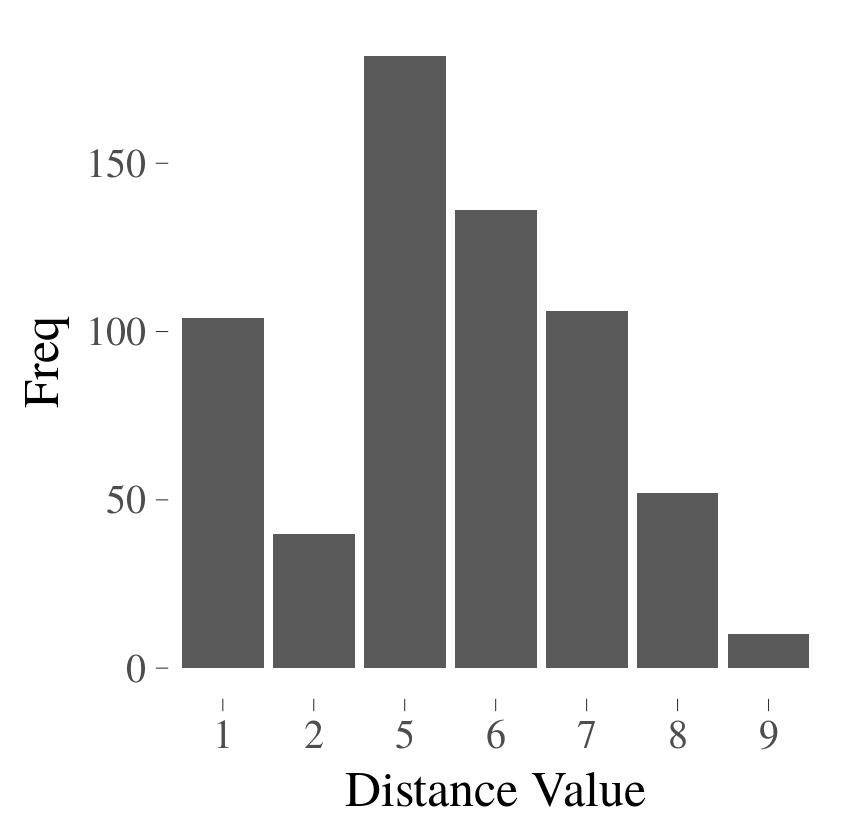
Histogram of original	Histogram after one multiplication
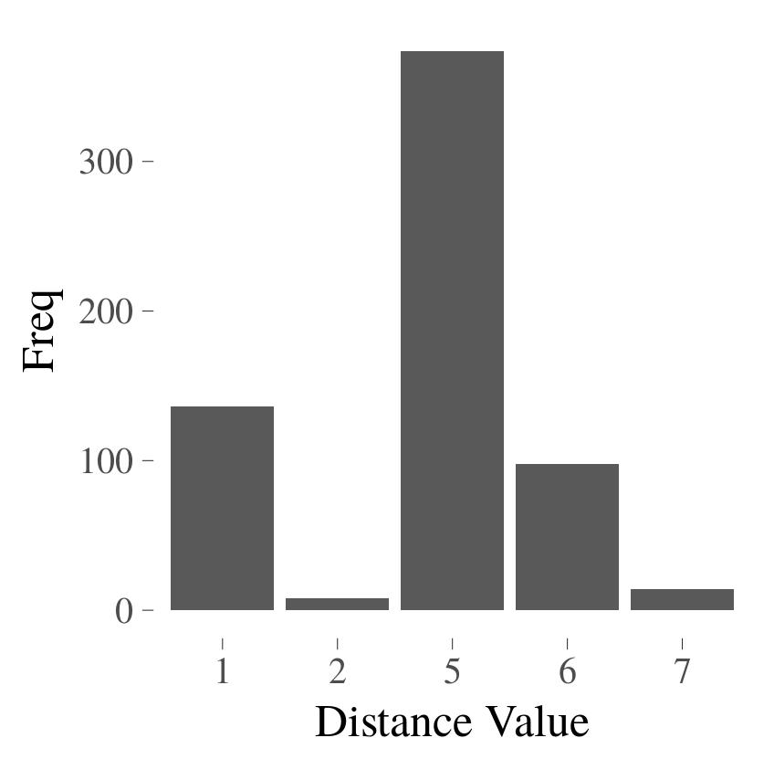
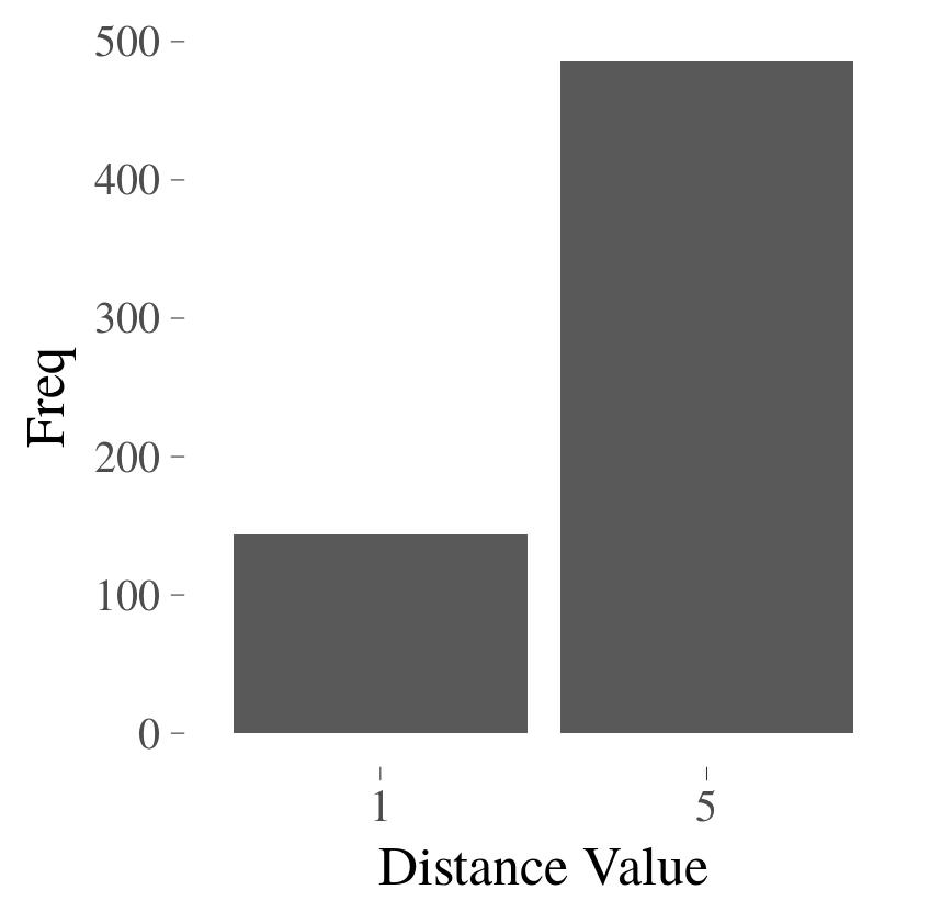
Histogram after two multiplications	Histogram after three multiplications

Figure 1: The process of distance equalization for successive powers of the incidence matrix. The matrix $A_{D}^{3}$ is ultrametric.

By shifting the data points to different locations, we create several distinct structured clusterings that consists of rectangular clusters.

Figures 2 and 3 show an example of a series of datasets with a total of 36 data points. Initially, the data set has 4 rectangular clusters containing 9 data points each with a gap of 3 distance units between the clusters. The ultrametricity of the dataset and, therefore, its clusterability is affected by the number of clusters, the size of the clusters, and the inter-cluster distances. Figure 3 shows that $m(A)$ reaches its highest value and, therefore, the clusterability is the lowest, when there is only one cluster in the dataset (see the third row of Figure 3).

Lattice with $k=4$	Histogram for $k=4$	$m(A_{D})=3,\textsf{clust}(D)=12$
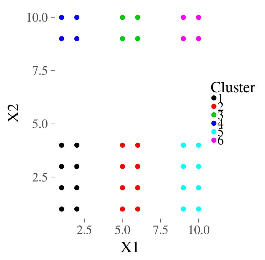
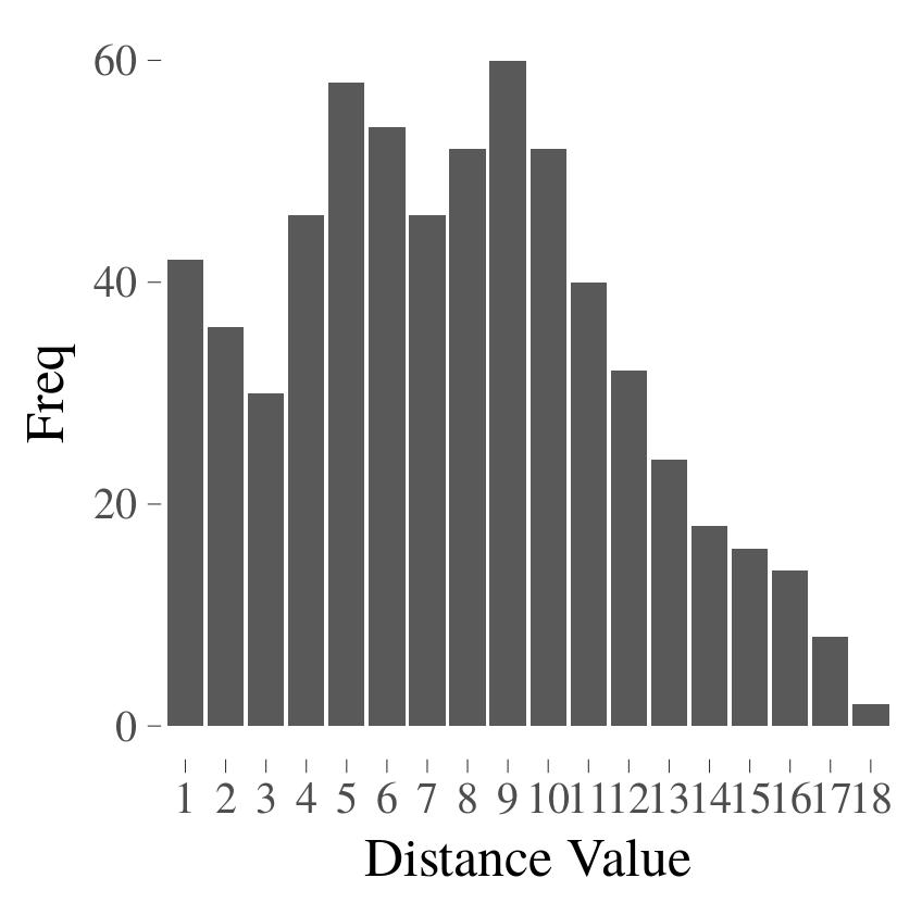
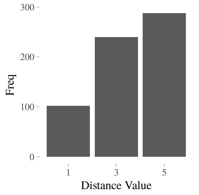
Lattice with $k=6$	Histogram for $k=6$	$m(A_{D})=4,\textsf{clust}(D)=9$
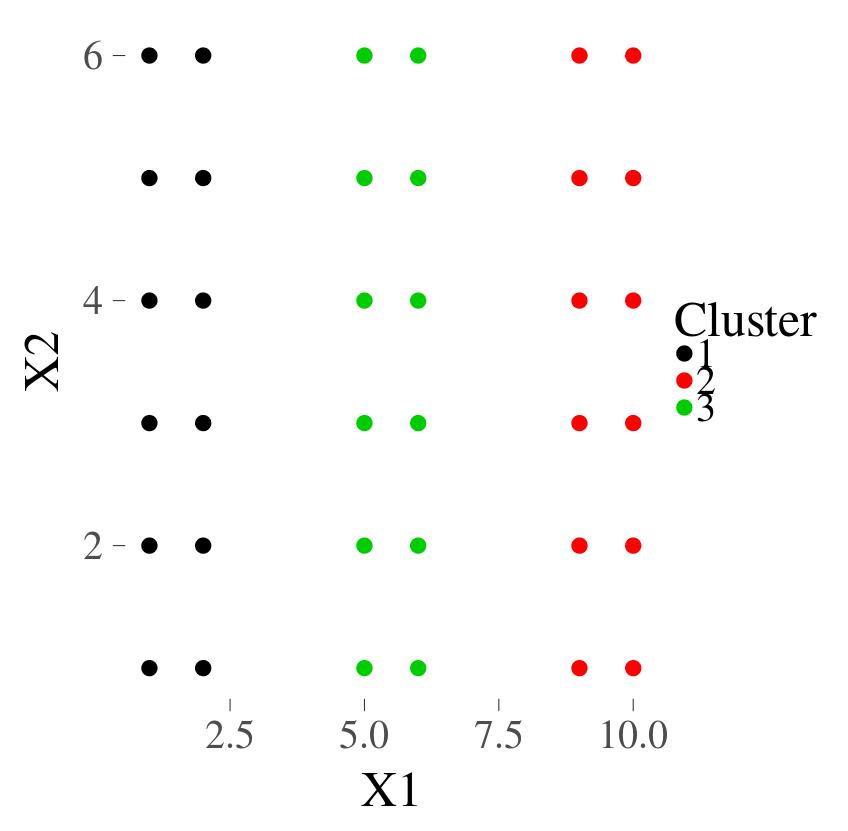
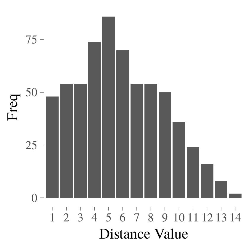
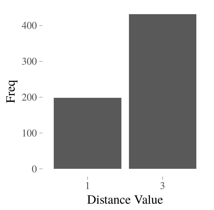
Lattice with $k=3$	Histogram for $k=3$	$m(A_{D})=5,\textsf{clust}(D)=7.2$

Figure 2: Cluster separation and clusterability.

If points are uniformly distributed, as it is the case in the third row of Figure 3, the clustering structure disappears and $\textsf{clust}(D)$ has the lowest value.

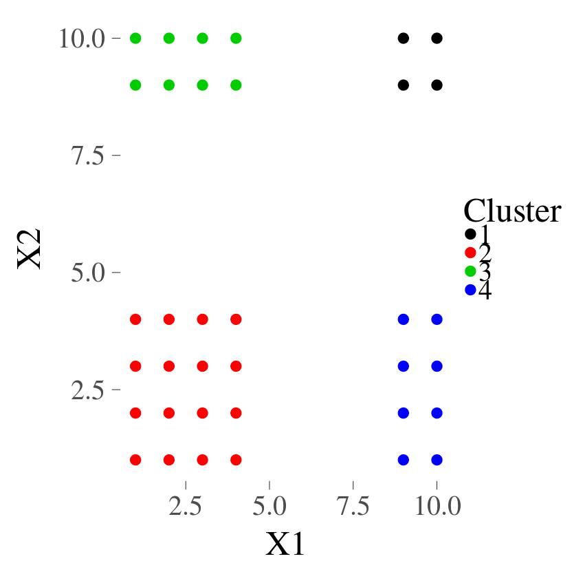
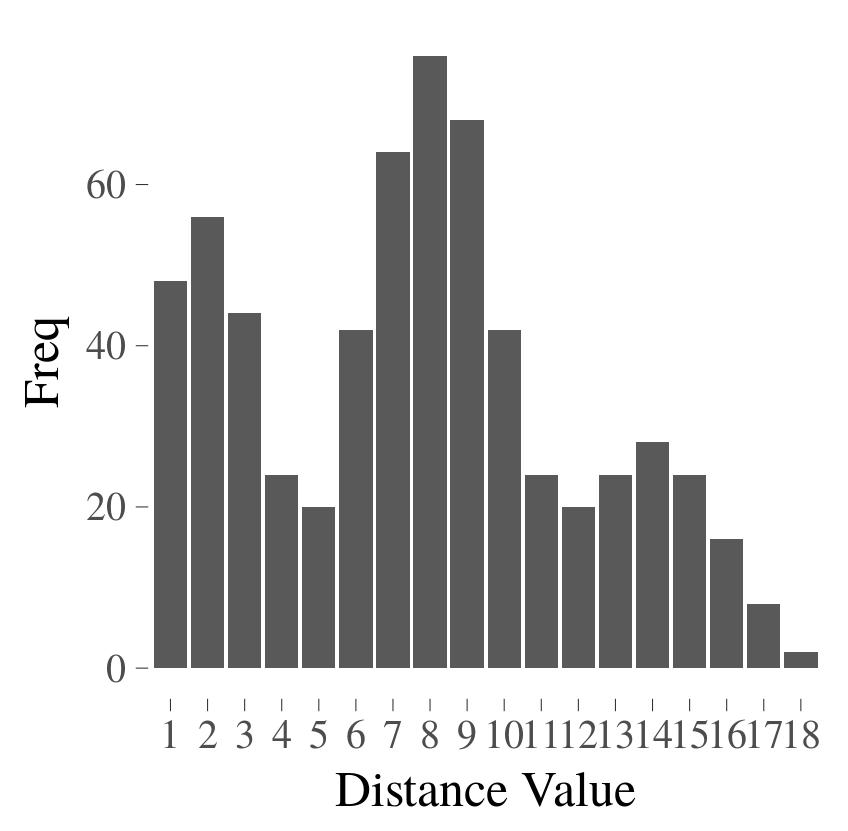
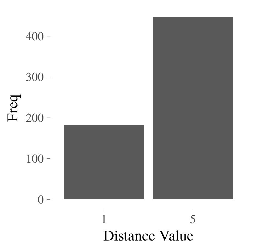
Lattice dataset with $k=4$	Histogram for $k=4$	$m(A_{D})=5,\textsf{clust}(D)=7.2$
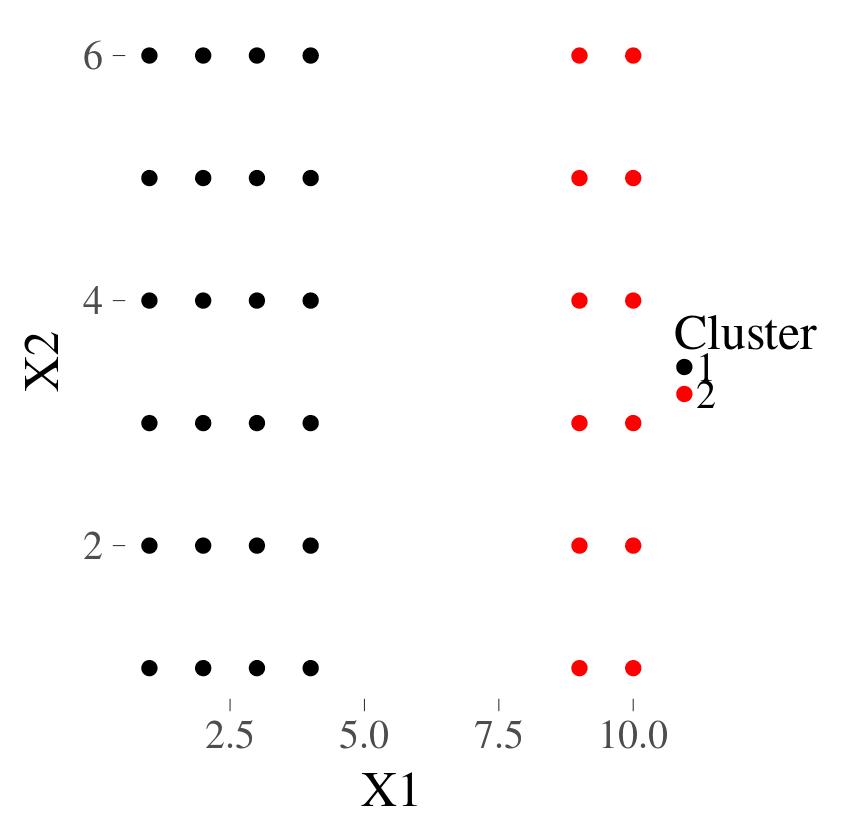
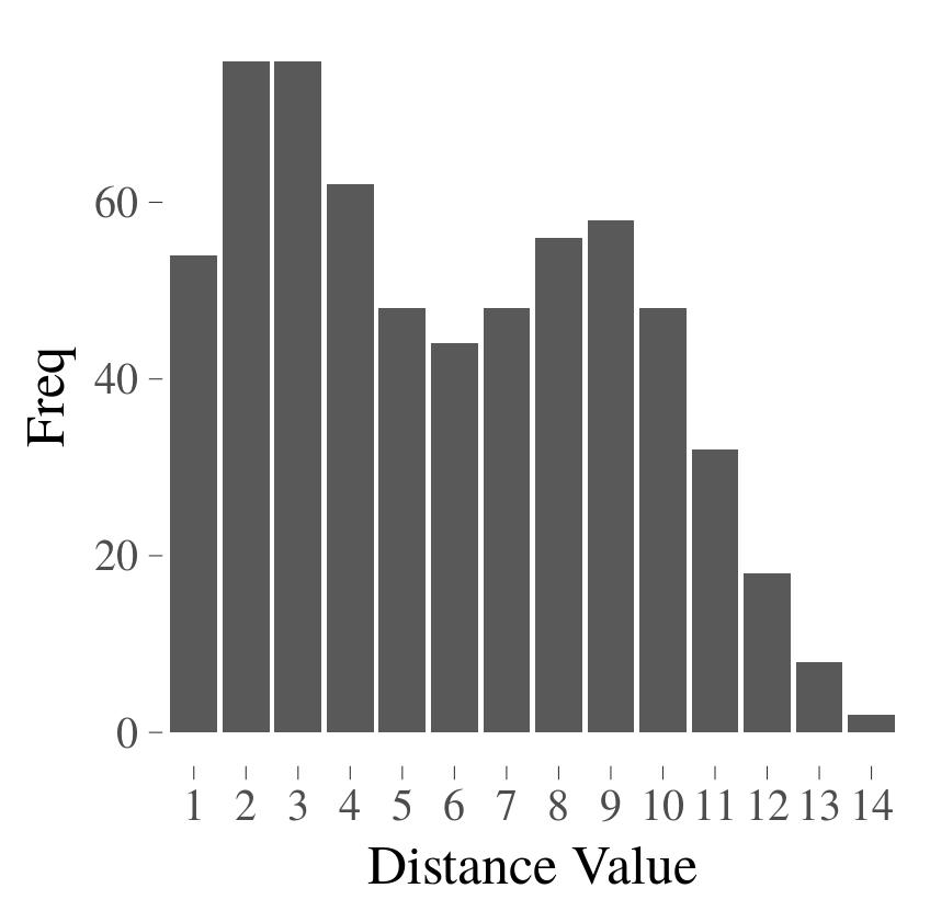
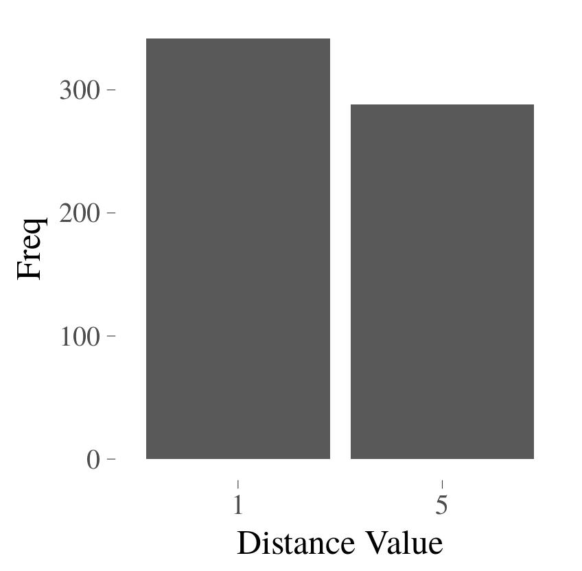
Lattice dataset with $k=2$	Histogram for $k=2$	$m(A_{D})=7,\textsf{clust}(D)=5.1$
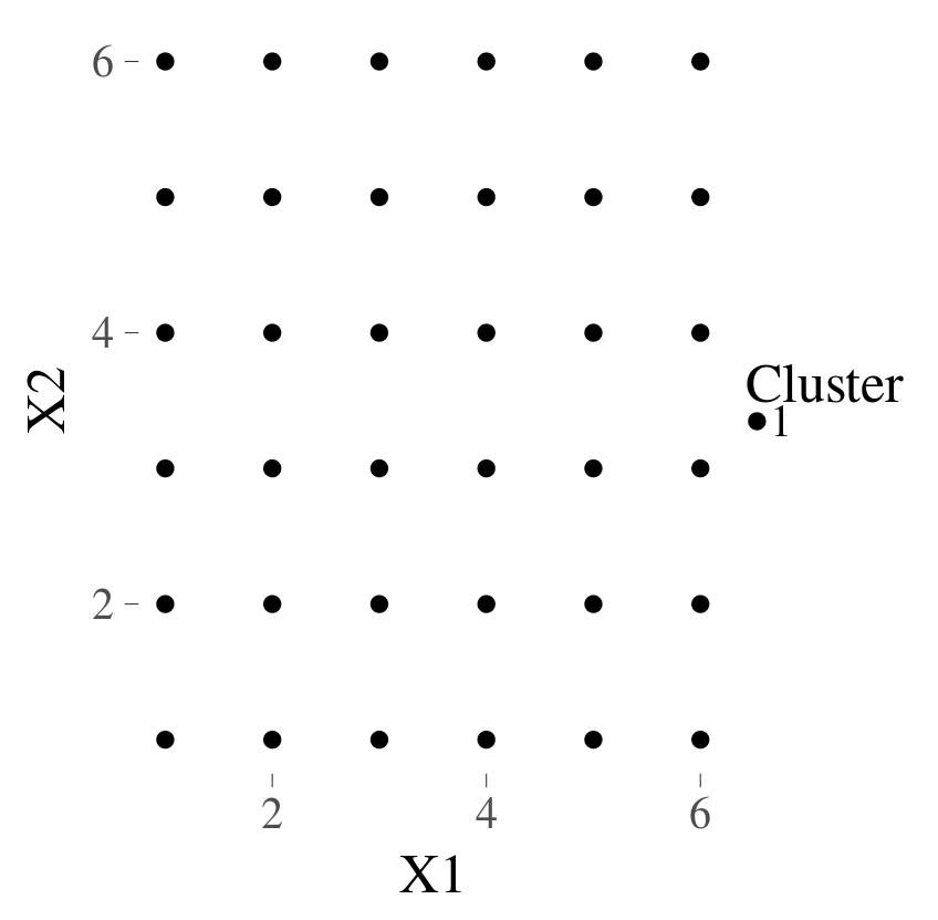
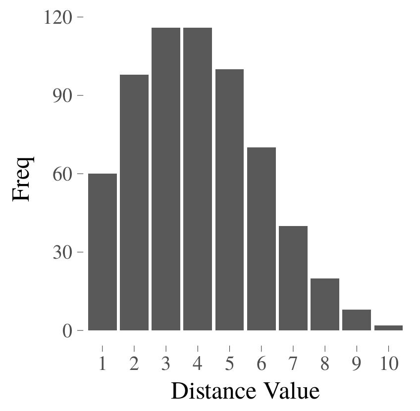
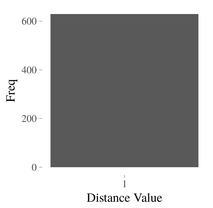
Lattice dataset with $k=1$	Histogram for $k=1$	$m(A_{D})=9,\textsf{clust}(D)=4$

Figure 3: Cluster separation and clusterability (continued).

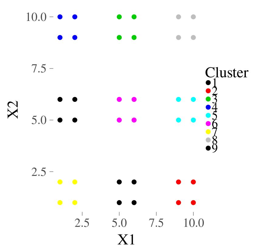
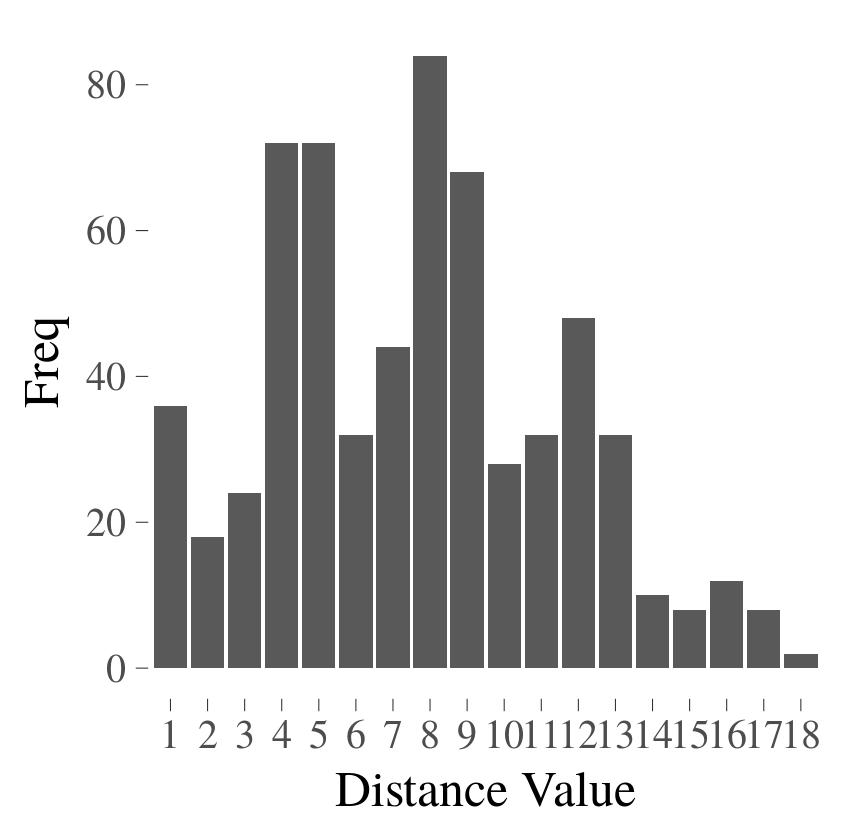
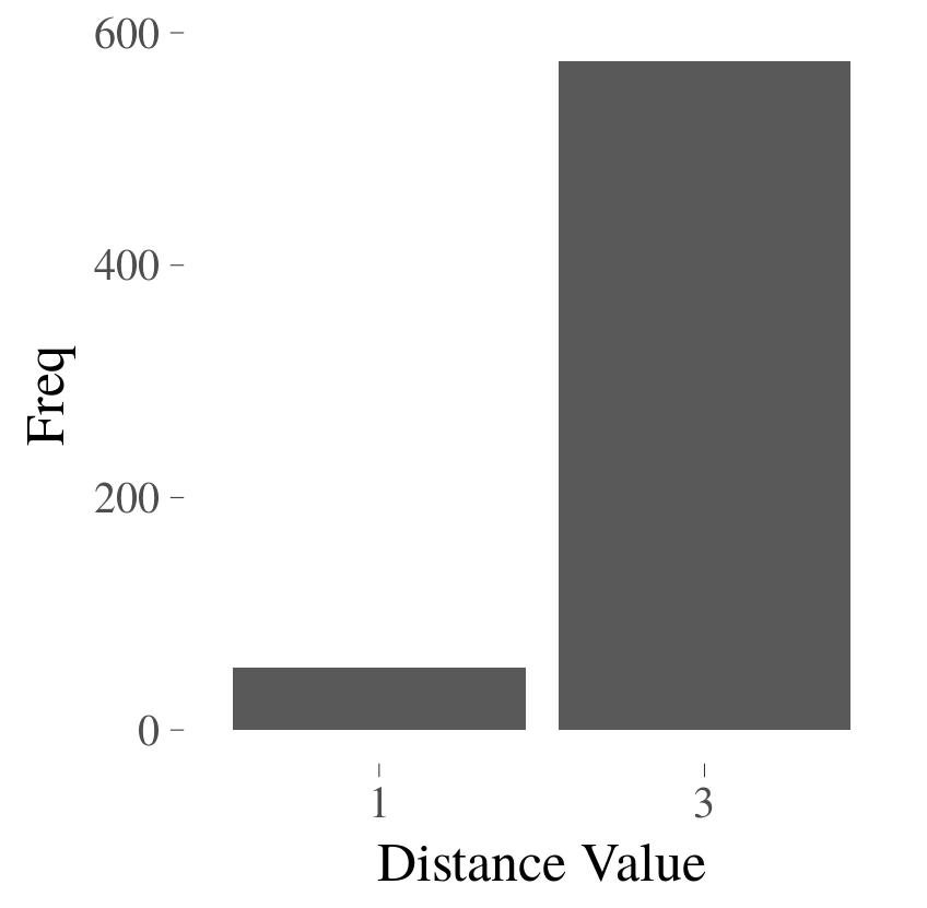
Lattice dataset with $k=9$	$k=9$	$m(A_{D})=6,\textsf{clust}(D)=6$

Figure 4: Further examples of data sets and their clusterability.

Histograms are used by some authors [10, 2] to identify the degree of clusterability. Note however that in the case of the data shown in Figures 2 and 3, the histograms of original dissimilarity of the dataset do not offer guidance on the clusterability(second column of Figure 2 and 3). By applying the “min-max” power operation on the original matrix, we get an ultrametric matrix. The new histogram of the ultrametric shows a clear difference on each dataset. In the third column of Figures 2 and 3, the histogram of the ultrametric matrix for each dataset shows a decrease of the number of distinct distances after the “power” operation.

If the dataset has no clustering structure the histogram of the ultrametric distance has only one bar.

The number of pics $p$ of the histogram indicate the minimum number of clusters $k$ in the ultrametric space specified by the matrix $A^{*}$ using the equality $\binom{k}{2}=p$, so the number of clusters is $\left\lceil\frac{1+\sqrt{1+8p}}{2}\right\rceil$. The largest $k$ values of valleys of the histogram indicate the radii of the spheres in the ultrametric space that define the clusters.

If a data set contains a large number of small clusters, these clusters can be regarded as outliers and the clusterability of the data set is reduced. This is the case in the third line of Figure 4 which shows a particular case for 9 clusters with 36 data points. Since the size of each cluster is too small to be considered as a real cluster, all of them together are merely regarded as a one cluster dataset with 9 points.

5 Conclusions and Future Work

The special matrix powers of the adjacency matrix of the weighted graph of object dissimilarities provide a tool for computing the subdominant ultrametric of a dissimilarity and an assessment of the existence of an underlying clustering structure in a dissimilarity space.

The “power” operation successfully eliminates the redundant information in the dissimilarity matrix of the dataset but maintains the useful information that can discriminate the cluster structures of the dataset.

In a series of seminal papers[15, 16, 17], F. Murtagh argued that as the dimensionality of a linear metric space increases, an equalization process of distances takes place and the metric of the space gets increasingly closer to an ultrametric. This raises the issues related to the comparative evaluation (statistical and algebraic) of the ultrametricity of such spaces and of their clusterability, which we intend to examine in the future.

References

References

- [1] M. Ackerman, A. Adolfsson, and N. Brownstein. An effective and efficient approach for clusterability evaluation. CoRR, abs/1602.06687, 2016.
- [2] M. Ackerman and S. Ben-David. Clusterability: A theoretical study. In Proceedings of the Twelfth International Conference on Artificial Intelligence and Statistics, AISTATS 2009, Clearwater Beach, Florida, USA, April 16-18, 2009, pages 1–8, 2009.
- [3] M. Ackerman, S. Ben-David, and D. Loker. Towards property-based classification of clustering paradigms. In Advances in Neural Information Processing Systems 23: 24th Annual Conference on Neural Information Processing Systems 2010. Proceedings of a meeting held 6-9 December 2010, Vancouver, British Columbia, Canada., pages 10–18.
- [4] Margareta Ackerman and Shai Ben-David. Clusterability: A theoretical study. In Proceedings of the Twelfth International Conference on Artificial Intelligence and Statistics, AISTATS 2009, Clearwater Beach, Florida, USA, April 16-18, 2009, pages 1–8, 2009.
- [5] Margareta Ackerman, Shai Ben-David, Simina Brânzei, and David Loker. Weighted clustering. In Proceedings of the Twenty-Sixth AAAI Conference on Artificial Intelligence, July 22-26, 2012, Toronto, Ontario, Canada., pages 858–863, 2012.
- [6] Andreas Adolfsson, Margareta Ackerman, and N. C. Brownstein. To cluster, or not to cluster: An analysis of clusterability methods. CoRR, abs/1808.08317, 2018.
- [7] M. F. Balcan, A. Blum, and S. Vempala. A discriminative framework for clustering via similarity functions. In Proceedings of the 40th Annual ACM Symposium on Theory of Computing, Victoria, British Columbia, Canada, May 17-20, 2008, pages 671–680, 2008.
- [8] S. Ben-David. Computational feasibility of clustering under clusterability assumptions. CoRR, abs/1501.00437.
- [9] S. Ben-David and M. Ackerman. Measures of clustering quality: A working set of axioms for clustering. In Advances in Neural Information Processing Systems 21, Proceedings of the Twenty-Second Annual Conference on Neural Information Processing Systems, Vancouver, British Columbia, Canada, December 8-11, 2008, pages 121–128, 2008.
- [10] S. Ben-David and M. Ackerman. Measures of clustering quality: A working set of axioms for clustering. In Advances in Neural Information Processing Systems 21, Proceedings of the Twenty-Second Annual Conference on Neural Information Processing Systems, Vancouver, British Columbia, Canada, December 8-11, 2008, pages 121–128, 2008.
- [11] A. Ben-Hur, A. Elisseeff, and I. Guyon. A stability based method for discovering structure in clustered data. In Proceedings of the 7th Pacific Symposium on Biocomputing, PSB 2002, Lihue, Hawaii, USA, January 3-7, 2002, pages 6–17, 2002.
- [12] Amit Daniely, Nati Linial, and Michael E. Saks. Clustering is difficult only when it does not matter. CoRR, abs/1205.4891, 2012.
- [13] S. Epter, M. Krishnamoorthy, and M. Zaki. Clusterability detection and initial seed selection in large datasets. In The International Conference on Knowledge Discovery in Databases, volume 7, 1999.
- [14] B. Leclerc. Description combinatoire des ultramétriques. Mathématiques et science humaines, 73:5–37, 1981.
- [15] Fionn Murtagh. Quantifying ultrametricity. In COMPSTAT, pages 1561–1568, 2004.
- [16] Fionn Murtagh. Clustering in very high dimensions. In UK Workshop on Computational Intelligence, page 226, 2005.
- [17] Fionn Murtagh. Identifying and exploiting ultrametricity. In Advances in Data Analysis, pages 263–272. Springer, 2007.
- [18] D. A. Simovici and C. Djeraba. Mathematical Tools for Data Mining – Set Theory, Partial Orders, Combinatorics. Springer-Verlag, London, second edition, 2008.