Statistical mechanics of self-gravitating systems in general relativity:
II. The classical Boltzmann gas

Abstract

We study the statistical mechanics of classical self-gravitating systems confined within a box of radius $R$ in general relativity. It has been found that the caloric curve $T_{\infty}(E)$ has the form of a double spiral whose shape depends on the compactness parameter $\nu=GNm/Rc^{2}$. The double spiral shrinks as $\nu$ increases and finally disappears when $\nu_{\rm max}=0.1764$. Therefore, general relativistic effects render the system more unstable. On the other hand, the cold spiral and the hot spiral move away from each other as $\nu$ decreases. Using a normalization $\Lambda=-ER/GN^{2}m^{2}$ and $\eta=GNm^{2}/Rk_{B}T_{\infty}$ appropriate to the nonrelativistic limit, and considering $\nu\rightarrow 0$, the hot spiral goes to infinity and the caloric curve tends towards a limit curve (determined by the Emden equation) exhibiting a single cold spiral, as found in former works. Using another normalization ${\cal M}=GM/Rc^{2}$ and ${\cal B}={Rc^{4}}/{GNk_{B}T_{\infty}}$ appropriate to the ultrarelativistic limit, and considering $\nu\rightarrow 0$, the cold spiral goes to infinity and the caloric curve tends towards a limit curve (determined by the general relativistic Emden equation) exhibiting a single hot spiral. This result is new. We discuss the analogies and the differences between this asymptotic caloric curve and the caloric curve of the self-gravitating black-body radiation. Finally, we compare box-confined isothermal models with heavily truncated isothermal distributions in Newtonian gravity and general relativity.

I Introduction

In a preceding paper theory1 (Paper I), relying on previous works on the subject tolman ; cocke ; hk0 ; kh ; khk ; kam ; kh2 ; hk ; ipser80 ; sorkin ; sy ; sy2 ; bvrelat ; aarelat1 ; aarelat2 ; gao ; gaoE ; roupas1 ; gsw ; fg ; roupas1E ; schiffrin ; psw ; fhj , we have developed a general formalism to study the statistical mechanics of self-gravitating systems in general relativity. This formalism is valid for an arbitrary form of entropy. The statistical equilibrium state is obtained by maximizing the entropy $S$ at fixed mass-energy $Mc^{2}$ and particle number $N$. The extremization problem yields the Tolman-Oppenheimer-Volkoff (TOV) equations tolman ; ov expressing the condition of hydrostatic equilibrium together with the Tolman-Klein relations tolman ; klein . The precise form of entropy determines the distribution function and the equation of state of the system. For illustration, in Paper I, we considered a system of self-gravitating fermions. In that case, the statistical equilibrium state is obtained by maximizing the Fermi-Dirac entropy at fixed mass-energy and particle number. This yields the relativistic Fermi-Dirac distribution function. In the present paper, we consider the statistical mechanics of classical self-gravitating particles. In that case, the statistical equilibrium state is obtained by maximizing the Boltzmann entropy at fixed mass-energy and particle number. This yields the relativistic Maxwell-Boltzmann (or Maxwell-Juttner) distribution function. We start by a brief history of the subject giving an exhaustive list of references.

The statistical mechanics of nonrelativistic classical self-gravitating systems was developed in connection with the dynamical evolution of globular clusters (see Appendix D of clm1 for a short review). Because of close two-body gravitational encounters between stars, globular clusters have the tendency to approach a Maxwell-Boltzmann distribution chandrabook . However, when coupled to gravity, the isothermal distribution has an infinite mass so that it cannot be valid everywhere in the cluster. In practice, the relaxation towards the Maxwell-Boltzmann distribution is hampered by the escape of high energy stars ambartsumian ; spitzer and the Maxwell-Boltzmann distribution is established only in the core of the system where stars have sufficiently negative energies. Since evaporation is a slow process, globular clusters can be found in quasiequilibrium states described by a truncated Maxwell-Boltzmann distribution – a Woolley distribution woolley or a King king distribution – whose parameters slowly evolve in time. The series of equilibria $T(E)$ has the form of a spiral (see Fig. 4 of Appendix A). Because of close encounters and evaporation, the system contracts and follows a series of equilibra $T(E)$ along which the energy $E$ decreases and the temperature $T$ increases (in the part of the caloric curve where the specific heat is negative) as the central density $\rho_{0}$ increases. The thermodynamical stability of the truncated Maxwell-Boltzmann distribution (Woolley and King models) has been studied in lbw ; katzking ; clm1 . At the turning point of energy (minimum energy), when the specific heat vanishes, passing from negative to positive values, the series of equilibria becomes unstable and the system undergoes the Antonov instability antonov , also known as the gravothermal catastrophe lbw , and collapses. This instability can be followed by using dynamical models based either on moment equations derived from the Fokker-Planck equation larson1 ; larson2 , Monte Carlo models hmc , heuristic fluid equations hnns ; lbe , or kinetic equations such as the orbit-averaged-Fokker-Planck equation cohn . During the collapse the system takes a core-halo structure in which the cluster develops a dense and hot core and a diffuse envelope. The dynamical evolution of the system is due to the gradient of temperature (velocity dispersion) between the core and the halo and the fact that the core has a negative specific heat. The core loses heat to the profit of the halo, becomes hotter, and contracts. If the temperature increases more rapidly in the core than in the halo there is no possible equilibrium and we get a thermal runaway: this is the gravothermal catastrophe. As a result, the core collapses and reaches higher and higher densities and higher and higher temperatures while the halo is not sensibly affected by the collapse of the core and maintains its initial structure. The collapse of the core is self-similar and leads to a finite-time singularity: the central density and the temperature become infinite in a finite time while the core radius shrinks to nothing lbe ; cohn . This is called core collapse. The mass contained in the core tends to zero at the collapse time. The evolution may continue in a self-similar postcollapse regime with the formation of a binary star inagakilb . The energy released by the binary can stop the collapse and induce a reexpansion of the system. Then, a series of gravothermal oscillations is expected to follow oscillations ; hr . It has to be noted that the gravothermal catastrophe is a thermodynamical instability, not a dynamical instabilty. Indeed, it has been shown that all the isotropic stellar systems with a distribution function of the form $f=f(\epsilon)$ with $f^{\prime}(\epsilon)<0$, like the truncated Maxwell-Boltzmann distribution, are dynamically stable with respect to a collisionless (Vlasov) evolution doremus71 ; doremus73 ; gillon76 ; sflp ; ks ; kandrup91 . In particular, all the isothermal configurations on the series of equilibria are dynamically stable, including those deep into the spiral that are thermodynamically unstable. Therefore, dynamical and thermodynamical stability do not coincide in Newtonian gravity (see Paper I for a more detailed discussion). As a result, the process of core collapse of globular clusters is a very long (secular) process, taking place on a collisional relaxation timescale of the order of the age of the Universe since it is due to two-body gravitational encounters.

As the density and the temperature of the core increase during the gravothermal catastrophe, the system may become relativistic. In that case, we have to consider the evolution of general relativistic star clusters. The series of equilibria of heavily truncated Maxwell-Boltzmann distributions in general relativity (relativistic Woolley model) was first studied by Zel’dovich and Podurets zp . They discovered the existence of a maximum temperature $k_{B}(T_{\infty})_{\rm max}/mc^{2}=0.273$ in the series of equilibria $T_{\infty}(\rho_{0})$ as the central density $\rho_{0}$, or the central redshift $z_{0}$, increases ($T_{\infty}$ is the temperature measured by an observer at infinity). They argued that the system should undergo a gravitational collapse at that point that they called an “avalanche-type catastrophic contraction of the system”. The mechanism of the collapse proposed by Zeldovich and Podurets zp is the following. At the maximum temperature the orbits of highly relativistic particles become unstable and the corresponding particles start falling in spirals towards the center. The collapse of the orbits of some particles leads to an increase of the field acting on the other particles, whose orbits collapse in turn etc. This catastrophic collapse occurs rapidly, on a dynamical timescale. A large fraction of the system (the main mass) rapidly contracts to its gravitational radius and forms what is now called a black hole (see footnote 3 in paper I). However, only the core of the system collapses. There remains a cloud surrounding the main mass. The particles in the cloud, following the laws of slow evolution, gradually fall into the collapsed mass.

The dynamical fackerell ; ipserthorne ; ipser69 ; ipser69b ; fackerell70 ; sudbury ; sf76 ; fs76 ; ipser80 ; mr ; mreuro ; mr90 ; bmrv ; bmrv2 and thermodynamical hk0 ; kh ; khk ; kam ; kh2 ; hk stability of heavily truncated Maxwell-Boltzmann (isothermal) distributions in general relativity have been studied by several authors. Ipser ipser69b ; ipser80 showed that dynamical and thermodynamical instabilities coincide in general relativity and that they occur at the turning point of the fractional binding energy $E/Nmc^{2}=(M-Nm)/Nm$, corresponding to a central redshift $z_{c}=0.516$. At that point $[(M-Nm)/Nm]_{\rm c}=0.0357$, $(Rc^{2}/2GNm)_{\rm c}=4.42$, and $(k_{B}T_{\infty}/mc^{2})_{\rm c}=0.23$. This critical point is different from the turning point of temperature reported by Zel’dovich and Podurets zp corresponding to $z_{0}=1.08$, $(M-Nm)/Nm=0.0133$, $Rc^{2}/2GNm=3.92$, and $k_{B}(T_{\infty})_{\rm max}/mc^{2}=0.27$. In particular, the gravitational instability occurs sooner than predicted by Zel’dovich and Podurets zp . This led to the following scenario proposed by Fackerell et al. fit which refines the former scenario of Zel’dovich and Podurets zp . They assumed that the evolution of relativistic spherical star clusters in the nuclei of some galaxies (which may have resulted from the gravothermal catastrophe of an initially Newtonian stellar system) proceeds quasistatically along a series of equilibria $T_{\infty}(E)$. The evolution is driven by stellar collisions and by the evaporation of stars. Both collision and evaporation drive the cluster toward states of higher and higher central density (or central redshift), higher and higher temperature (in the region of negative specific heat) and lower and lower binding energy. When the cluster reaches the turning point of fractional binding energy (minimum fractional binding energy) it can no longer evolve quasistatically and it undergoes a dynamical instability of general relativistic origin. Relativistic gravitational collapse sets it: the stars spiral inward through the gravitational radius of the cluster towards its center leaving behind a “black hole” in space with some stars orbiting it. Fackerell et al. fit speculated that violent events in the nuclei of galaxies and in quasars might be associated with the onset of such a collapse or with encounters between an already collapsed cluster (black hole) and surrounding stars.

This scenario has been confirmed by Shapiro and Teukolsky st1 ; st2 ; st3 ; st4 ; kochanek ; rst1 ; strevue who numerically solved the relativistic Vlasov-Einstein equations describing the dynamical evolution of a collisionless spherical gas of particles in general relativity. They specifically considered star clusters made of compact stars such as white dwarfs, neutron stars or stellar mass black holes. At the centers of the galaxies the collisions may be sufficient to induce a dynamical evolution. Begining from a dense, but otherwise Newtonian, star cluster, and following secular core concentration on a two-body relaxation time scale (i.e. the gravothermal catastrophe), the cluster may develop an extreme core-halo configuration. Therefore, if relativistic star clusters form in nature they are likely to be very centrally condensed. Because of collisions and evaporation, the central density, the central redshift and the central velocity dispersion increase. Shapiro and Teukolsky st2 (see also rst1 ) followed the series of equilibria of truncated isothermal distributions and showed from direct numerical simulations that above a critical redshift $z_{c}\sim 0.5$, corresponding to the turning point of fractional binding energy, the relativistic star cluster becomes dynamically unstable and undergoes a catastrophic collapse to a supermassive black hole on a dynamical time scale. Even in the case of extremely centrally condensed configurations with extensive Newtonian halo, an appreciable fraction of the total cluster mass collapses to the central black hole st4 ; kochanek . This happens even when the initial central core is just a small fraction of the total mass. This occurs because of the “avalanche effect” predicted by Zel’dovich and Podurets zp according to which the particles in the cloud gradually fall into the collapsed mass. Shapiro and Teukolsky argued st3 that the collapse of such clusters embedded in evolved galactic nuclei can lead to the formation of supermassive black holes of the “right size” ($10^{6}\leq M/M_{\odot}\leq 10^{9}$) to explain quasars and active galactic nuclei (AGNs).

In a later work, Balberg et al. balberg (see also bash ; pss ) applied similar ideas to self-interacting dark matter. Namely, they developed, in the context of dark matter, the idea of “avalanche-type contraction” towards a supermassive black hole initially suggested by Zel’dovich and Podurets zp , improved by Fackerell et al. fit , and confirmed numerically by Shapiro and Teukolsky st2 ; st3 ; st4 . They argued that dark matter halos experience a gravothermal catastrophe and that, when the central density and the temperature increase above a critical value, the system undergoes a dynamical instability of general relativistic origin leading to the formation of a supermassive black hole on a dynamical timescale. The dynamical evolution of the system is due to the self-interaction of the dark matter particles. In that case, a typical halo has sufficient time to thermalize and acquire a gravothermal profile consisting of a flat core surrounded by an extended halo. There is a first stage in which the halo is in the long mean free path (LMFP) limit. It undergoes a gravothermal catastrophe in which the core collapses self-similarly. This is analogous (with slightly different exponents) to the self-similar collapse of globular clusters. In this process, the core mass decreases rapidly. If this self-similar evolution were going to completion then, when the core becomes relativistic, it would contain almost no mass. So, even if it collapsed by a dynamical relativistic instability, it would not form a supermassive black hole. But during the gravothermal catastrophe, the core of self-interacting dark matter halos passes in the short mean free path (SMFP) limit. In the SMFP limit, the core mass decreases more slowly (and almost saturates) so that a relatively large mass can ultimately collapse into a supermassive black hole. We note that only the central region of a dark matter halo (not its outer part) is affected by this process so the final outcome of this scenario is an isothermal halo harboring a central supermassive black hole. In recent works, we have proposed to apply this scenario to isothermal models of dark matter halos made of fermions clm1 ; clm2 or bosons bosons .

In the previously mentioned studies, the star clusters are described by the truncated Maxwell-Boltzmann distribution. In that case, the link with standard thermodynamics is not straightforward because the truncated Maxwell-Boltzmann distribution differs from the ordinary Maxwell-Boltzmann distribution and describes an out-of-equilibrium situation where some stars leave the system. Using the truncated Maxwell-Boltzmann distribution is compulsory if we want to describe realistic star clusters since the ordinary Maxwell-Boltzmann distribution coupled to gravity has an infinite mass. However, it may be useful to study in parallel simplified models (somewhat academic) that correspond to standard statistical mechanics based on the ordinary Maxwell-Boltzmann distribution. This can be done by confining artificially the particles within a spherical box with reflecting boundary conditions in order to have a finite mass. This “box model” was introduced by Antonov antonov in the case of nonrelativistic stellar systems. The statistical mechanics of nonrelativistic classical self-gravitating systems confined within a box has been studied by numerous authors antonov ; lbw ; ipser74 ; tvh ; hkpart1 ; nakada ; hs ; hk3 ; katzpoincare1 ; ih ; inagaki ; lecarkatz ; ms ; sflp ; lp ; kiessling ; paddyapj ; paddy ; dvsc ; semelin0 ; katzokamoto ; semelin ; dvs1 ; dvs2 ; aaiso ; crs ; sc ; grand ; katzrevue ; lifetime ; ijmpb ; sb . These studies have been extended in general relativity by Katz and Horwitz kh2 and more recently by Roupas roupas and Alberti and Chavanis acb . The caloric curves (more precisely the series of equilibria) giving the normalized inverse temperature $\eta=GNm^{2}/Rk_{B}T_{\infty}$ as a function of the normalized energy $\Lambda=-ER/GN^{2}m^{2}$, where $E=(M-Nm)c^{2}$ is the binding energy, depend on a unique parameter $\nu=GNm/Rc^{2}$ called the compactness parameter. It is found that the caloric curves generically present a double spiral. This double spiral shrinks as $\nu$ increases and finally disappears at the maximum compactness $\nu_{\rm max}=0.1764$. Therefore, general relativistic effects render the system more unstable roupas ; acb .

The “cold spiral” corresponds to weakly relativistic configurations. It is a relativistic generalization of the results obtained by Antonov antonov , Lynden-Bell and Wood lbw and Katz katzpoincare1 for the nonrelativistic classical gas. Indeed, in the nonrelativistic limit $\nu\rightarrow 0$, if we use the normalized variables $\Lambda=-ER/GN^{2}m^{2}$ and $\eta=GNm^{2}/Rk_{B}T_{\infty}$, the hot spiral is rejected at infinity and we recover the results of antonov ; lbw ; katzpoincare1 . The caloric curve $\eta(\Lambda)$ has a spiral (snail-like) structure (see Fig. 3 of katzpoincare1 ). In the microcanonical ensemble the system undergoes a gravothermal catastrophe below a minimum energy $E_{c}=-0.335\,GM^{2}/R$, corresponding to a density contrast ${\cal R}_{\rm MCE}=\rho(0)/\rho(R)=709$. This leads to a binary star surrounded by a hot halo inagakilb . In the canonical ensemble, it undergoes an isothermal collapse below a minimum temperature $T_{c}=GMm/(2.52Rk_{B})$, corresponding to a density contrast ${\cal R}_{\rm CE}=32.1$. This leads to a Dirac peak containing all the particles post .

The “hot spiral” corresponds to strongly relativistic configurations. It is related (but not identical) to the caloric curve of the box-confined self-gravitating black-body radiation obtained by Sorkin et al. sorkin and Chavanis aarelat2 , which also has the form of a spiral (see Fig. 15 of aarelat2 ). For the self-gravitating black-body radiation the system undergoes a gravitational collapse (presumably towards a black hole) above a maximum energy ${M}_{\rm max}c^{2}=0.246\,Rc^{4}/G$ in the microcanonical ensemble, corresponding to an energy density contrast ${\cal R}_{\rm MCE}=\epsilon(0)/\epsilon(R)=22.4$, or above a maximum temperature $k_{B}(T_{\infty})_{\rm max}=0.445\,(\hbar^{3}c^{7}/GR^{2})^{1/4}$ in the canonical ensemble, corresponding to an energy density contrast ${\cal R}_{\rm CE}=\epsilon(0)/\epsilon(R)=1.91$. In Sec. VI of this paper, we discuss in detail the connection between the hot spiral of the general relativistic classical gas and of the self-gravitating black-body radiation. We show that for $\nu\rightarrow 0$, if we use the normalized variables ${\cal M}=GM/Rc^{2}$ and ${\cal B}=Rc^{4}/GNk_{B}T_{\infty}$, instead of $\Lambda$ and $\eta$, the cold spiral is rejected at infinity. In that case, the caloric curve of the general relativistic classical self-gravitating gas tends to a limit curve ${\cal B}({\cal M})$ which has a spiral (snail-like) structure. The hot spiral corresponds to ultrarelativistic configurations. The maximum mass $M_{\rm max}=0.246\,Rc^{2}/G$ and the corresponding energy density contrast $22.4$ are the same as for the self-gravitating black-body radiation obtained in sorkin ; aarelat2 but the maximum temperature $k_{B}T_{\rm max}=0.0561\,Rc^{4}/GN$ and the corresponding energy density contrast $10.3$ are different from the self-gravitating black-body radiation because they have a different physical origin.

The paper is organized as follows. In Sec. II we develop the statistical mechanics of nonrelativistic self-gravitating classical particles. In Sec. III we develop the statistical mechanics of general relativistic classical particles. In Sec. IV we present a scaling argument showing that the caloric curve of general relativistic classical particles depends on a unique control parameter $\nu=GNm/Rc^{2}$ (compactness parameter). Generically, the caloric curve has the form of a double spiral. In Sec. V we consider the nonrelativistic limit and show that, when $\nu\rightarrow 0$, the normalized caloric curve $\eta(\Lambda)$ tends towards a limit curve exhibiting a single cold spiral, as found in former works antonov ; lbw ; katzpoincare1 . In Sec. VI we consider the ultrarelativistic limit and show that, when $\nu\rightarrow 0$, the normalized caloric curve ${\cal B}({\cal M})$ tends towards a limit curve exhibiting a single hot spiral. This asymptotic curve has not been reported previously. We discuss the analogies and the differences between this asymptotic caloric curve and the caloric curve of the self-gravitating black-body radiation sorkin ; aarelat2 . Finally, in Appendices A and B we compare box-confined isothermal models with heavily truncated isothermal distributions in Newtonian gravity and general relativity.

II Statistical mechanics of nonrelativistic self-gravitating classical particles

In this section, we consider the statistical mechanics of nonrelativistic self-gravitating classical particles. The formalism and the notations are the same as in Sec. II of Paper I in the case of fermions. We shall not repeat the equations that are identical. The only difference is that we are considering classical particles described by the Boltzmann entropy density

$$s(r) = -k_{B}\int f\left[\ln\left(\frac{f}{f_{*}}\right)-1\right]\,{d}{\bf p}.$$ (1)

The Boltzmann entropy can be obtained from a combinatorial analysis. It is equal to the logarithm of the number of microstates (complexions) corresponding to a given macrostate (see ijmpb for details). A microstate is characterized by the specification of the position ${\bf r}_{i}$ and the impulse ${\bf p}_{i}$ of all the particles ($i=1,...,N$). A macrostate is characterized by the (smooth) distribution function $f({\bf r},{\bf p})$ giving the density of particles in the macrocell (${\bf r},{\bf r}+d{\bf r};{\bf p},{\bf p}+d{\bf p})$, irrespectively of their precise position in the cell. Since a classical system is “diluted” in phase space, we do not have to put any constraint on the possible microstates. The combinatorial analysis then directly leads to the Boltzmann entropy (1) where $f_{*}$ is a constant introduced for dimensional reasons (it is related to the size $h$ of a microcell). If the particles are fermions, as in Paper I, the Boltzmann entropy (1) can also be obtained by expanding the Fermi-Dirac entropy (I-22) for $f\ll f_{\rm max}$, where $f_{\rm max}=g/h^{3}$ is the maximum possible value of the distribution function fixed by the Pauli exclusion principle ($h$ is the Planck constant and $g$ is the spin multiplicity of quantum states). This establishes $f_{*}=f_{\rm max}$. More generally, all the results of the present paper (which are valid for classical particles) can be obtained from the results of Paper I (which are valid for fermions) by considering the nondegenerate limit $f\ll f_{\rm max}$. However, the present formalism is more general since it can also describe a gas of bosons far from the condensation point ($T\gg T_{c}$). We recall that a statistical equilibrium state exists only if the system is confined within a box of radius $R$ otherwise it would evaporate (see, e.g., Ref. sc for details). We shall therefore consider the “box model” as in Paper I.

II.1 Maximization of the entropy density at fixed kinetic energy density and particle number density

In the microcanonical ensemble, the statistical equilibrium state is obtained by maximizing the entropy $S$ at fixed energy $E$ and particle number $N$. As in Paper I, we proceed in two steps. We first maximize the Boltzmann entropy density $s(r)$ at fixed kinetic energy density $\epsilon_{\rm kin}(r)$ and particle number density $n(r)$ with respect to variations on $f({\bf r},{\bf p})$. This leads to the Maxwell-Boltzmann distribution function

$$f({\bf r},{\bf p})=\frac{g}{h^{3}}e^{-\beta(r)p^{2}/2m+\alpha(r)},$$ (2)

where $\beta(r)$ and $\alpha(r)$ are local Lagrange multipliers. Introducing the local temperature $T(r)$ and the local chemical potential $\mu(r)$ through the relations $\beta(r)=1/k_{B}T(r)$ and $\alpha(r)=\mu(r)/k_{B}T(r)$, the Maxwell-Boltzmann distribution (2) can be rewritten as

$$f({\bf r},{\bf p})=\frac{g}{h^{3}}e^{-[p^{2}/2m-\mu(r)]/k_{B}T(r)}.$$ (3)

It corresponds to the condition of local thermodynamical equilibrium. Substituting the Maxwell-Boltzmann distribution (3) into Eqs. (I-17), (I-18) and (I-20), and performing the Gaussian integrations, we get

$$n(r)=\frac{g}{h^{3}}[2\pi mk_{B}T(r)]^{3/2}e^{\mu(r)/k_{B}T(r)},$$ (4)

$$\epsilon_{\rm kin}(r)=\frac{3}{2}n(r)k_{B}T(r),$$ (5)

$$P(r)=\frac{2}{3}\epsilon_{\rm kin}(r)=n(r)k_{B}T(r),$$ (6)

where we recall that the first equality in Eq. (6) is valid for an arbitrary nonrelativistic perfect gas, whatever its distribution function (see Appendix A of Paper I). On the other hand, the second equality of Eq. (6) is the famous Boyle’s law of a classical gas. These equations relate the Lagrange multipliers $\beta(r)$ and $\alpha(r)$, or the thermodynamical variables $T(r)$ and $\mu(r)$, to the constraints $\epsilon_{\rm kin}(r)$ and $n(r)$. Substituting the Maxwell-Boltzmann distribution (3) into the entropy density (1) we obtain the integrated Gibbs-Duhem relation (I-37). It is shown in Appendix E of Paper I that this relation is valid for an arbitrary form of entropy. For the Boltzmann entropy, using Eqs. (5) and (6), the integrated Gibbs-Duhem relation (I-37) reduces to the form

$$\frac{s(r)}{k_{B}}=\frac{5}{2}n(r)-\alpha(r)n(r).$$ (7)

Using Eq. (4) it can also be written as

$$\frac{s(r)}{k_{B}}=\frac{5}{2}n(r)-n(r)\ln n(r)-n(r)\ln\left(\frac{h^{3}}{g}\right)+\frac{3}{2}n(r)\ln[2\pi mk_{B}T(r)].$$ (8)

This equation provides an expression of the entropy density for a classical system of particles in local thermodynamic equilibrium.

II.2 Maximization of the entropy at fixed energy and particle number

We now maximize the entropy $S$ at at fixed energy $E$ and particle number $N$ with respect to variations on $n(r)$ and $\epsilon_{\rm kin}(r)$. Here, we just consider the extremization problem (see Appendix C for more general results). As shown in Paper I, it leads to the relations

$$\beta=\frac{1}{k_{B}T}\qquad{\rm and}\qquad\alpha(r)=\alpha_{0}-\beta m\Phi(r),$$ (9)

where $\beta=1/(k_{B}T)$ and $\alpha_{0}$ are constant. Therefore, at statistical equilibrium the temperature is uniform and the chemical potential is given by the Gibbs law

$$\mu(r)=\mu_{0}-m\Phi(r)$$ (10)

with $\mu_{0}=\alpha_{0}k_{B}T$. The Gibbs law expresses the fact that the total chemical potential $\mu_{\rm tot}\equiv\mu(r)+m\Phi(r)$ is uniform at statistical equilibrium. Substituting these relations into Eqs. (2) and (3), we obtain the mean field Maxwell-Boltzmann distribution function

$$f({\bf r},{\bf p})=\frac{g}{h^{3}}e^{\alpha_{0}}e^{-\beta({p}^{2}/2m+m\Phi(r))}.$$ (11)

This result can also be directly obtained by extremizing the entropy $S$ at at fixed energy $E$ and particle number $N$ with respect to variations on $f({\bf r},{\bf p})$ as detailed in Appendix C of Paper I. The local variables become

$$n(r)=\frac{g}{h^{3}}e^{\alpha_{0}}\left(\frac{2\pi m}{\beta}\right)^{3/2}e^{-\beta m\Phi(r)},$$ (12)

$$\epsilon_{\rm kin}(r)=\frac{3}{2}n(r)k_{B}T,$$ (13)

$$P(r)=n(r)k_{B}T,$$ (14)

$$\frac{s(r)}{k_{B}}=\frac{5}{2}n(r)-\alpha_{0}n(r)+\beta n(r)m\Phi(r),$$ (15)

$$\frac{s(r)}{k_{B}}=\frac{5}{2}n(r)-n(r)\ln n(r)-n(r)\ln\left(\frac{h^{3}}{g}\right)+\frac{3}{2}n(r)\ln(2\pi mk_{B}T).$$ (16)

These equations characterize a barotropic gas with a linear equation of state $P(r)=n(r)k_{B}T$. Using Eq. (12), the distribution function (11) can be written in terms of the density as

$$f({\bf r},{\bf p})=n({r})\left(\frac{\beta}{2\pi m}\right)^{3/2}e^{-\beta{p}^{2}/2m}.$$ (17)

On the other hand, the energy (kinetic $+$ potential) and the entropy are given by

$$E=E_{\rm kin}+W=\frac{3}{2}Nk_{B}T+\frac{1}{2}\int\rho(r)\Phi(r)\,d{V},$$ (18)

$$S=-\frac{\mu_{0}}{T}N+\frac{5}{2}Nk_{B}+\frac{2W}{T},$$ (19)

where $\rho(r)=n(r)m$ is the mass density. We recall that the condition of statistical equilibrium, corresponding to the extremization of the entropy at fixed energy and particle number, implies the condition of hydrostatic equilibrium (see Appendix D of Paper I). This is valid for a general form of entropy. In the present case, this can be checked immediately by taking the gradient of the pressure given by Eq. (14) and using Eq. (12).

II.3 Canonical ensemble: Minimization of the free energy at fixed particle number

In the previous sections, we considered the microcanonical ensemble. In the canonical ensemble, the statistical equilibrium state is obtained by minimizing the free energy

$$F=E-TS$$ (20)

at fixed particle number $N$. Proceeding similarly to Sec. II.F of Paper I, we get the same results as in Secs. II.1 and II.2 (for the first variations). At statistical equilibrium, using Eqs. (18) and (19), the free energy is given by

$$F=\mu_{0}N-W-Nk_{B}T.$$ (21)

III Statistical mechanics of general relativistic classical particles

In this section, we consider the statistical mechanics of self-gravitating classical particles within the framework of general relativity. The formalism and the notations are the same as in Sec. III of Paper I but now the entropy density is given by the Boltzmann entropy density (1) instead of the Fermi-Dirac entropy density (I-121). As in the Newtonian case, a statistical equilibrium state exists only if the system is confined within a box of radius $R$ otherwise it would evaporate.

III.1 Maximization of the entropy density at fixed energy density and particle number density

In the microcanonical ensemble, the statistical equilibrium state is obtained by maximizing the entropy $S$ at fixed mass-energy $Mc^{2}$ and particle number $N$. As in Paper I, we proceed in two steps. We first maximize the entropy density at fixed energy density $\epsilon(r)$ and particle number density $n(r)$ with respect to variations on $f({\bf r},{\bf p})$. This leads to the relativistic Maxwell-Boltzmann (or Maxwell-Juttner) distribution function

$$f({\bf r},{\bf p})=\frac{g}{h^{3}}e^{-\beta(r)E(p)+\alpha(r)},$$ (22)

where $\beta(r)$ and $\alpha(r)$ are local Lagrange multipliers. Introducing the temperature and the chemical potential through the relations $\beta(r)=1/k_{B}T(r)$ and $\alpha(r)=\mu(r)/k_{B}T(r)$, it can be rewritten as

$$f({\bf r},{\bf p})=\frac{g}{h^{3}}e^{-[E(p)-\mu(r)]/k_{B}T(r)}.$$ (23)

This corresponds to the condition of local thermodynamical equilibrium. The local variables are

$$n(r)=\frac{g}{h^{3}}\int e^{-[E(p)-\mu(r)]/{k_{B}T(r)}}\,d{\bf p},$$ (24)

$$\epsilon(r)=\frac{g}{h^{3}}\int e^{-[E(p)-\mu(r)]/{k_{B}T(r)}}E\,d{\bf p},$$ (25)

$$\epsilon_{\rm kin}(r)=\frac{g}{h^{3}}\int e^{-[E(p)-\mu(r)]/{k_{B}T(r)}}E_{\rm kin}(p)\,d{\bf p},$$ (26)

$$P(r)=\frac{g}{3h^{3}}\int e^{-[E(p)-\mu(r)]/k_{B}T(r)}p\frac{{d}E}{{d}p}\,{d}{\bf p}.$$ (27)

Using an integration by parts in the last equation, we get

$$P(r)=n(r)k_{B}T(r).$$ (28)

This is the same equation of state as for a nonrelativistic gas (Boyle’s law). This result was first established by Juttner juttner1 ; juttner2 but is implicit in the work of Planck planck . Eqs. (24) and (25) determine the Lagrange multipliers $\beta(r)$ and $\alpha(r)$, or the thermodynamical variables $T(r)$ and $\mu(r)$, in terms of $\epsilon(r)$ and $n(r)$. Substituting the Maxwell-Juttner distribution function (23) into Eq. (1), and using Eq. (24)-(28), we obtain the integrated Gibbs-Duhem relation (I-135). It is shown in Appendix E of Paper I that this relation is valid for an arbitrary form of entropy. For the Boltzmann entropy, using Eq. (28), the integrated Gibbs-Duhem relation (I-135) reduces to the form

$$s(r)=\frac{\epsilon(r)-\mu(r)n(r)}{T(r)}+k_{B}n(r).$$ (29)

III.2 Maximization of the entropy at fixed mass-energy and particle number

We now maximize the entropy $S$ at at fixed energy $E$ and particle number $N$ with respect to variations on $n(r)$ and $\epsilon(r)$. Here, we just consider the extremization problem. As shown in Paper I, it leads to the relation

$$\alpha=\frac{\mu(r)}{k_{B}T(r)}=\frac{\mu_{\infty}}{k_{B}T_{\infty}},$$ (30)

where $\alpha$ is a constant ($\mu_{\infty}$ and $T_{\infty}$ are the chemical potential and the temperature measured by an observer at infinity). The extremization problem also yields the TOV equations [see Eqs. (I-155) and (I-156)] expressing the condition of hydrostatic equilibrium and the Tolman-Klein relations [see Eqs. (I-158) and (I-159)]. We recall that, in general relativity, the temperature $T(r)$ depends on the position even at statistical equilibrium. This is the so-called Tolman effect tolman . Using Eqs. (29) and (30), we find that the entropy is given at statistical equilibrium by

$$S=\int_{0}^{R}\frac{\epsilon(r)}{T(r)}\left[1-\frac{2GM(r)}{rc^{2}}\right]^{-1/2}4\pi r^{2}\,dr+k_{B}N-\frac{\mu_{\infty}}{T_{\infty}}N.$$ (31)

III.3 Canonical ensemble: Minimization of the free energy at fixed particle number

In the previous sections, we considered the microcanonical ensemble. In the canonical ensemble, the statistical equilibrium state is obtained by minimizing the free energy

$$F=E-T_{\infty}S$$ (32)

at fixed particle number $N$. Proceeding similarly to Sec. III.F of Paper I, we get the same results as in Secs. III.1 and III.2. At statistical equilibrium, the free energy is given by

$$F=(M-Nm)c^{2}-\int_{0}^{R}\frac{T_{\infty}}{T(r)}\epsilon(r)\left[1-\frac{2GM(r)}{rc^{2}}\right]^{-1/2}4\pi r^{2}\,dr-k_{B}T_{\infty}N+\mu_{\infty}N.$$ (33)

III.4 Equations determining the statistical equilibrium state in terms of $T(r)$

III.4.1 Local variables in terms of $T(r)$ and $\alpha$

Using Eq. (30), we can rewrite the distribution function (22) or (23) and the local variables (24)-(27) as

$$f({\bf r},{\bf p})=\frac{g}{h^{3}}e^{\alpha}e^{-E(p)/k_{B}T(r)},$$ (34)

$$n(r)=\frac{g}{h^{3}}e^{\alpha}\int e^{-E(p)/k_{B}T(r)}\,d{\bf p},$$ (35)

$$\epsilon(r)=\frac{g}{h^{3}}e^{\alpha}\int e^{-E(p)/k_{B}T(r)}E\,d{\bf p},$$ (36)

$$\epsilon_{\rm kin}(r)=\frac{g}{h^{3}}e^{\alpha}\int e^{-E(p)/k_{B}T(r)}E_{\rm kin}(p)\,d{\bf p},$$ (37)

where we recall that $\alpha$ is a constant while the temperature $T(r)$ depends on the position (Tolman’s effect). The pressure is given by Eq. (28).

III.4.2 Juttner transformation

In special relativity, the energy of a particle is $E(p)=\sqrt{p^{2}c^{2}+m^{2}c^{4}}$. Making the Juttner transformation juttner1 ; juttner2 ; chandrabook

$$\frac{p}{mc}=\sinh\theta,$$ (38)

we find that $E=mc^{2}\cosh\theta$. We also introduce the normalized local inverse temperature

$$b(r)=\frac{mc^{2}}{k_{B}T(r)}.$$ (39)

With the transformation (38), Eqs. (35)-(37) become

$$n(r)=\frac{4\pi gm^{3}c^{3}}{h^{3}}e^{\alpha}\int_{0}^{+\infty}e^{-b(r)\cosh\theta}\sinh^{2}\theta\cosh\theta\,d\theta,$$ (40)

$$\epsilon(r)=\frac{4\pi gm^{4}c^{5}}{h^{3}}e^{\alpha}\int_{0}^{+\infty}e^{-b(r)\cosh\theta}\sinh^{2}\theta\cosh^{2}\theta\,d\theta,$$ (41)

$$\epsilon_{\rm kin}(r)=\frac{4\pi gm^{4}c^{5}}{h^{3}}e^{\alpha}\int_{0}^{+\infty}e^{-b(r)\cosh\theta}\sinh^{2}\theta\cosh\theta(\cosh\theta-1)\,d\theta.$$ (42)

They can be expressed in terms of the modified Bessel functions defined by

$$K_{n}(z)=\int_{0}^{+\infty}e^{-z\cosh\theta}\cosh(n\theta)\,d\theta.$$ (43)

For future reference, we recall their asymptotic behaviors:

$$K_{n}(z)\sim\frac{1}{2}\frac{(n-1)!}{\left(\frac{1}{2}z\right)^{n}}\qquad(z\rightarrow 0),$$ (44)

$$K_{n}(z)\simeq\left(\frac{\pi}{2z}\right)^{1/2}e^{-z}\left(1+\frac{4n^{2}-1}{8z}+...\right)\qquad(z\rightarrow+\infty).$$ (45)

The nonrelativistic limit ($k_{B}T\ll mc^{2}$) corresponds to $z\rightarrow+\infty$ and the ultrarelativistic limit ($k_{B}T\gg mc^{2}$) corresponds to $z\rightarrow 0$. Using the relations

$$\sinh^{2}\theta\cosh\theta=\frac{1}{4}[\cosh(3\theta)-\cosh\theta],$$ (46)

$$\sinh^{2}\theta\cosh^{2}\theta=\frac{1}{8}[\cosh(4\theta)-1],$$ (47)

and the recurrence formula

$$K_{n-1}(z)-K_{n+1}(z)=-\frac{2n}{z}K_{n}(z),$$ (48)

we can write the local variables as

$$n(r)=\frac{4\pi gm^{3}c^{3}}{h^{3}}e^{\alpha}\frac{1}{b(r)}K_{2}(b(r)),$$ (49)

$$\epsilon(r)=\frac{4\pi gm^{4}c^{5}}{h^{3}}e^{\alpha}\frac{1}{b(r)}K_{2}(b(r))\left[\frac{K_{1}(b(r))}{K_{2}(b(r))}+\frac{3}{b(r)}\right],$$ (50)

$$\epsilon_{\rm kin}(r)=\frac{4\pi gm^{4}c^{5}}{h^{3}}e^{\alpha}\frac{1}{b(r)}K_{2}(b(r))\left[\frac{K_{1}(b(r))}{K_{2}(b(r))}+\frac{3}{b(r)}-1\right],$$ (51)

$$P(r)=n(r)\frac{mc^{2}}{b(r)}.$$ (52)

On the other hand, using Eq. (49), the distribution function (34) can be written in terms of the density as

$$f({\bf r},{\bf p})=\frac{n(r)}{4\pi m^{3}c^{3}}\frac{b(r)}{K_{2}(b(r))}e^{-b(r)E(p)/mc^{2}}.$$ (53)

This expression, which can be compared to Eq. (17) in the nonrelativistic case, is tricky because the factor in front of the exponential is independent of $r$ [see Eq. (34)]. The spatial inhomogeneity of the system due to the self-gravity manifests itself in the temperature $T(r)$ as discussed in Paper I.

III.4.3 Equation of state

From Eqs. (49)-(51) we can write

$$\epsilon_{\rm kin}(r)=n(r)mc^{2}{\cal F}(b(r)),\qquad\epsilon(r)=n(r)mc^{2}\left[1+{\cal F}(b(r))\right],$$ (54)

where we have introduced the function aarelat1 :

$${\cal F}(z)=\frac{K_{1}(z)}{K_{2}(z)}+\frac{3}{z}-1.$$ (55)

Its asymptotic behaviors are

$${\cal F}(z)\sim\frac{3}{z}\qquad(z\rightarrow 0),$$ (56)

$${\cal F}(z)\sim\frac{3}{2z}\qquad(z\rightarrow+\infty).$$ (57)

Using Eqs. (52) and (54), we get

$$P(r)=\frac{\epsilon(r)}{b(r)[1+{\cal F}(b(r))]}.$$ (58)

Since $b(r)$ is related to $\epsilon(r)$ through Eq. (50), the foregoing equation can be viewed as an equation of state relating the pressure to the energy density. It is important to note, however, that this relation also depends on $\alpha$, so that it is of the form $P(r)=P(\epsilon(r),\alpha)$.

The ratio between the pressure and the kinetic energy density is

$$\frac{P(r)}{\epsilon_{\rm kin}(r)}=\frac{1}{b(r){\cal F}(b(r))}.$$ (59)

In the nonrelativistic limit $b\rightarrow+\infty$ ($k_{B}T\ll mc^{2}$), using Eq. (57), we get

$$\frac{P(r)}{\epsilon_{\rm kin}(r)}\rightarrow\frac{2}{3}.$$ (60)

In the ultrarelativistic limit $b\rightarrow 0$ ($k_{B}T\gg mc^{2}$), using Eq. (56), we get

$$\frac{P(r)}{\epsilon_{\rm kin}(r)}\rightarrow\frac{1}{3}.$$ (61)

This returns the general results from Appendix A of Paper I which are valid for an arbitrary distribution function.

III.4.4 The TOV equations in terms of $T(r)$

Using the general results of Paper I, the TOV equations can be written in terms of $T(r)$ as

$$\frac{dM}{dr}=\frac{\epsilon}{c^{2}}4\pi r^{2},$$ (62)

$$\frac{1}{T}\frac{{d}T}{{d}r}=-\frac{1}{c^{2}}\frac{\frac{GM(r)}{r^{2}}+\frac{4\pi G}{c^{2}}Pr}{1-\frac{2GM(r)}{rc^{2}}},$$ (63)

with the boundary conditions

$$M(0)=0\qquad{\rm and}\qquad T(0)=T_{0}.$$ (64)

For a given value of $\alpha$ and $T_{0}$ one can solve Eqs. (62) and (63) between $r=0$ and $r=R$ with the local variables given by Eqs. (49)-(52). The particle number constraint

$$N=\int_{0}^{R}n(r)\left[1-\frac{2GM(r)}{rc^{2}}\right]^{-1/2}4\pi r^{2}\,dr$$ (65)

can be used to determine $T_{0}$ as a function of $\alpha$ (there may be several solutions for the same value of $\alpha$). The total mass $M$ and the temperature $T_{\infty}$ measured by an observer at infinity are then obtained from the relations

$$M=M(R)\qquad{\rm and}\qquad T_{\infty}=T(R)\sqrt{1-\frac{2GM}{Rc^{2}}}.$$ (66)

In this manner, we get the binding energy $E=(M-Nm)c^{2}$ and the Tolman (global) temperature $T_{\infty}$ as a function of $\alpha$. By varying $\alpha$ between $-\infty$ and $+\infty$, we can obtain the full caloric curve $T_{\infty}(E)$ for a given value of $N$ and $R$ (we show in Sec. IV.1 that the results depend only on the ratio $N/R$). Finally, the entropy and the free energy are given by Eqs. (31) and (33).

III.4.5 The TOV equations in terms of $\varphi(r)$

Introducing the gravitational potential $\varphi(r)$ through the relation (see Paper I):

$$\frac{k_{B}T(r)}{mc^{2}}=\frac{1}{b(r)}=\frac{1}{|\alpha|}\sqrt{1+\frac{\varphi(r)}{c^{2}}},$$ (67)

we can rewrite the local variables (34)-(37) in terms of $\alpha$ and $\varphi(r)$. We can also directly substitute the relation (67) into the Juttner equations (49)-(52). On the other hand, the TOV equations can be written in terms of $\varphi(r)$ as (see Paper I):

$$\frac{dM}{dr}=\frac{\epsilon}{c^{2}}4\pi r^{2},$$ (68)

$$\frac{d\varphi}{dr}=-\frac{2G}{c^{2}}\left[\frac{\varphi(r)}{c^{2}}+1\right]\frac{M(r)c^{2}+4\pi P(r)r^{3}}{r^{2}\left[1-\frac{2GM(r)}{rc^{2}}\right]},$$ (69)

with the boundary conditions

$$M(0)=0\qquad{\rm and}\qquad\varphi(0)=\varphi_{0}>-c^{2}.$$ (70)

For a given value of $\alpha$ and $\varphi_{0}$ we can solve Eqs. (68) and (69) between $r=0$ and $r=R$ with the local variables obtained from Eqs. (49)-(52) and (67). The particle number constraint

$$N=\int_{0}^{R}n(r)\left[1-\frac{2GM(r)}{rc^{2}}\right]^{-1/2}4\pi r^{2}\,dr$$ (71)

can be used to determine $\varphi_{0}$ as a function of $\alpha$ (there may be several solutions for the same value of $\alpha$). The total mass $M$ and the temperature $T_{\infty}$ measured by an observer at infinity are then obtained from the relations

$$M=M(R)\qquad{\rm and}\qquad\frac{k_{B}T_{\infty}}{mc^{2}}=\frac{1}{|\alpha|}\sqrt{\frac{\varphi(R)}{c^{2}}+1}\left(1-\frac{2GM}{Rc^{2}}\right)^{1/2}.$$ (72)

In this manner, we get the binding energy $E=(M-Nm)c^{2}$ and the Tolman (global) temperature $T_{\infty}$ as a function of $\alpha$. By varying $\alpha$ between $-\infty$ and $+\infty$, we can obtain the full caloric curve $T_{\infty}(E)$ for a given value of $N$ and $R$ (we show in Sec. IV.1 that the results depend only on the ratio $N/R$). Finally, the entropy and the free energy are given by Eqs. (31) and (33) with Eq. (67).

IV General case: The double spiral

In this section, we discuss general properties of the caloric curve of general relativistic classical particles. A more detailed discussion is given in roupas ; acb .

IV.1 The $N/R$ scaling

We first show that, for classical particles, the normalized caloric curve determined by the equations of Sec. III.4 depends only on the ratio $N/R$ instead of $N$ and $R$ individually as in the case of fermions (Paper I). If we introduce the scaled variables

$$\tilde{r}=\frac{r}{R},\qquad\tilde{M}(\tilde{r})=\frac{GM(r)}{Rc^{2}},\qquad\tilde{\epsilon}(\tilde{r})=\frac{GR^{2}\epsilon(r)}{c^{4}},\qquad\tilde{P}(\tilde{r})=\frac{GR^{2}P(r)}{c^{4}},$$ (73)

$$\tilde{n}(\tilde{r})=\frac{GR^{2}n(r)m}{c^{2}},\qquad\tilde{N}(\tilde{r})=\frac{GN(r)m}{Rc^{2}},\qquad\tilde{\alpha}=\alpha+\ln\left(\frac{Gm^{4}cR^{2}}{h^{3}}\right)$$ (74)

in the equations of Sec. III.4, we find that the local variables (49)-(52) become

$$\tilde{n}(\tilde{r})=4\pi ge^{\tilde{\alpha}}\frac{1}{b(\tilde{r})}K_{2}(b(\tilde{r})),$$ (75)

$$\tilde{\epsilon}(\tilde{r})=4\pi ge^{\tilde{\alpha}}\frac{1}{b(\tilde{r})}K_{2}(b(\tilde{r}))\left[\frac{K_{1}(b(\tilde{r}))}{K_{2}(b(\tilde{r}))}+\frac{3}{b(\tilde{r})}\right],$$ (76)

$$\tilde{P}(\tilde{r})=\tilde{n}(\tilde{r})\frac{1}{b(\tilde{r})}.$$ (77)

On the other hand, the TOV equations (62) and (63) become

$$\frac{d\tilde{M}}{d\tilde{r}}=4\pi\tilde{\epsilon}(\tilde{r}){\tilde{r}}^{2},$$ (78)

$$\frac{db}{d\tilde{r}}=b(\tilde{r})\frac{\tilde{M}(\tilde{r})+4\pi\tilde{P}(\tilde{r}){\tilde{r}}^{3}}{{\tilde{r}}^{2}\left[1-\frac{2\tilde{M}(\tilde{r})}{\tilde{r}}\right]},$$ (79)

with the boundary conditions

$$\tilde{M}(0)=0,\qquad b(0)=b_{0}\geq 0.$$ (80)

The particle number constraint (65) takes the form

$$\tilde{N}=\int_{0}^{1}\tilde{n}(\tilde{r})\left[1-\frac{2G\tilde{M}(\tilde{r})}{\tilde{r}c^{2}}\right]^{-1/2}4\pi{\tilde{r}}^{2}\,{d}\tilde{r}.$$ (81)

Finally, the mass and the inverse Tolman temperature $\beta_{\infty}=1/k_{B}T_{\infty}$ [see Eq. (66)] are given by

$$\tilde{M}=\tilde{M}(1),\qquad b_{\infty}=b(1)\left(1-2\tilde{M}\right)^{-1/2}.$$ (82)

In this manner, we see that the problem depends only on the dimensionless number

$$\nu=\frac{GNm}{Rc^{2}},$$ (83)

corresponding to $\tilde{N}$. This is the so-called compactness parameter. It can be interpreted as the ratio $\nu=R_{S}^{*}/R$ between the effective Schwarzschild radius $R_{S}^{*}=GNm/c^{2}$, defined in terms of the rest mass $Nm$, and the box radius $R$. Alternatively, it can be interpreted as the ratio $\nu=Nm/M_{S}^{*}$ between the rest mass $Nm$ and the effective Schwarzschild mass $M_{S}^{*}=Rc^{2}/G$ defined in terms of the box radius. For a given value of $\nu$ (i.e. $\tilde{N}$), we can solve the dimensionless equations (75)-(82) and determine

$${\cal M}=\frac{GM}{Rc^{2}}\qquad{\rm and}\qquad b_{\infty}=\frac{mc^{2}}{k_{B}T_{\infty}},$$ (84)

where ${\cal M}$ corresponds to $\tilde{M}$. As a result, for a given value of $\nu$, we can plot the caloric curve giving $b_{\infty}$ as a function of ${\cal M}$. Actually, in order to make the link with the nonrelativistic limit $c\rightarrow+\infty$, it is preferable to plot

$$\eta=\frac{\beta_{\infty}GNm^{2}}{R}=\frac{GNm^{2}}{k_{B}T_{\infty}R}$$ (85)

as a function of

$$\Lambda=-\frac{ER}{GN^{2}m^{2}}=-\frac{(M-Nm)c^{2}R}{GN^{2}m^{2}},$$ (86)

where $E=(M-Nm)c^{2}$ is the binding energy (see Paper I). We have the relations

$$\Lambda=-\frac{{\cal M}-\nu}{\nu^{2}},\qquad\eta=b_{\infty}\nu.$$ (87)

In terms of the variables $\eta$ and $\Lambda$, the nonrelativistic caloric curve is recovered in the limit $\nu\rightarrow 0$ (see Sec. V).

Remark: The scaling of this section amounts to taking $m=c=G=R=h=1$ in the original equations. In that case, the normalized caloric curve is obtained by plotting $\eta=\beta_{\infty}N$ as a function of $\Lambda=-E/N^{2}$ for a given value of $N$ acb . We note, however, that the entropy introduces a new dependence in $R$. Indeed, the entropy and free energy scale as

$$S=\frac{Rc^{2}}{Gm}k_{B}\tilde{S}-Nk_{B}\ln\left(\frac{Gm^{4}cR^{2}}{h^{3}}\right),$$ (88)

$$F=\frac{Rc^{4}}{G}\tilde{F}+Nk_{B}T_{\infty}\ln\left(\frac{Gm^{4}cR^{2}}{h^{3}}\right),$$ (89)

where

$$\tilde{S}=\int_{0}^{1}\tilde{\epsilon}(\tilde{r})b(\tilde{r})\left[1-\frac{2\tilde{M}(\tilde{r})}{\tilde{r}}\right]^{-1/2}4\pi{\tilde{r}}^{2}\,d\tilde{r}+\tilde{N}-\tilde{\alpha}\tilde{N},$$ (90)

and

$$\tilde{F}=\tilde{M}-\tilde{N}-\frac{\tilde{S}}{b_{\infty}}.$$ (91)

We see on Eq. (88) that the entropy involves a contribution $-Nk_{B}\ln(R^{2})$ scaling like the logarithm of the area of the system. However, this term appears just as an additive constant in the entropy so it can be omitted in most applications.

IV.2 Description of the caloric curve

In Fig. 1 we have plotted the caloric curve of a general relativistic classical self-gravitating gas for a typical value of $\nu$ (specifically $\nu=0.1$). It has the form of a double spiral parametrized by the energy density contrast ${\cal R}=\epsilon(0)/\epsilon(R)$ roupas ; acb . The density contrast ${\cal R}$ is minimum at the “center” of the caloric curve and increases along the series of equilibria in the two directions as we approach the spirals.

The cold spiral (on the right) is a relativistic generalization of the caloric curve obtained by Katz katzpoincare1 for a nonrelativistic self-gravitating classical gas in Newtonian gravity (see Sec. V). It corresponds to weakly relativistic configurations (except when $\nu$ is large). It exhibits a minimum energy (in the microcanonical ensemble) at $E_{c}$ and a minimum temperature (in the canonical ensemble) at $T_{c}$ below which the system undergoes a gravitational collapse as in the case of nonrelativistic systems. If the system is sufficiently relativistic ($\nu$ large), the collapse may lead to the formation of a black hole. On the other hand, the hot spiral is a purely general relativity result. It is similar (but not identical) to the caloric curve obtained by Chavanis aarelat2 for the self-gravitating black-body radiation (see Sec. VI). It corresponds to strongly relativistic configurations. It exhibits a maximum energy (in the microcanonical ensemble) at $E_{\rm max}$ and a maximum temperature (in the canonical ensemble) at $T_{\rm max}$ above which the system undergoes a gravitational collapse leading presumably to the formation of a black hole.

In the canonical ensemble the series of equilibria is stable on the main branch between $\eta_{\rm min}$ and $\eta_{c}$. According to the Poincaré criterion poincare , it becomes unstable at the first turning points of temperature when the specific heat becomes infinite, passing from positive to negative values. A new mode of instability is lost at each subsequent turning point of temperature as the spirals rotate clockwise. In the microcanonical ensemble the series of equilibria is stable on the main branch between $\Lambda_{\rm min}$ and $\Lambda_{c}$. According to the Poincaré criterion poincare , it becomes unstable at the first turning points of energy when the specific heat vanishes, passing from negative to positive values. A new mode of instability is lost at each subsequent turning point of energy as the spirals rotate clockwise. There are two regions of ensembles inequivalence (one on each spiral), between the turning points of temperature and energy, i.e., in the first regions of negative specific heat.

It has to be noted that the stable equilibrium states are in fact metastable, as there is no global maximum of entropy or global minimum of free energy for classical self-gravitating systems antonov ; lbw . However, these metastable states have tremendously long lifetimes, scaling as $e^{N}$, so they are stable in practice lifetime .

The evolution of the caloric curve with $\nu$ is described in detail in roupas ; acb . As $\nu$ increases, the cold and hot spirals approach each other, merge at $\nu^{\prime}_{S}=0.128$, form a loop above $\nu_{S}=0.1415$, reduce to a point at $\nu_{\rm max}=0.1764$, and finally disappear. The limit $\nu\rightarrow 0$ is discussed in detail in the following sections.

According to Ipser’s conjecture ipser80 (see Paper I and footnote 5), dynamical and thermodynamical stability coincide in general relativity. However, as discussed in Paper I and footnote 5, we expect that the growth rate of the dynamical instability is small for weakly relativistic configurations (cold spiral) and large for strongly relativistic configurations (hot spiral). In other words, the collapse at $E_{c}$ is essentially a thermodynamical instability that takes place on a secular timescale while the collapse at $E_{\rm max}$ is essentially a dynamical instability taking place on a short timescale.

Figure 1: Caloric curve of a general relativistic self-gravitating classical gas for $\nu=0.1$. It presents a double spiral. The system collapses at low energies and low temperatures as in the case of a nonrelativistic self-gravitating classical gas (cold spiral). It also collapses (presumably towards a black hole) at high energies and high temperatures as in the case of the self-gravitating black-body radiation (hot spiral).

V Nonrelativistic limit: the cold spiral

The nonrelativistic limit of the classical isothermal gas corresponds to $k_{B}T\ll mc^{2}$. It can be formally obtained by taking the limits $T\rightarrow 0$, $b\rightarrow+\infty$, or $c\rightarrow+\infty$ in the equations of Sec. III. Proceeding as in Sec. IV of Paper I, we recover the results of Sec. II.

V.1 Differential equation for $\rho(r)$

The equation of state of a nonrelativistic classical gas at statistical equilibrium is given by [see Eq. (14)]:

$$P(r)=\rho(r)\frac{k_{B}T}{m}.$$ (92)

This is the classical isothermal equation of state chandrabook . Substituting this equation of state into the fundamental equation of hydrostatic equilibrium (I-8), we obtain the following differential equation

$$\frac{1}{r^{2}}\frac{d}{dr}\left(r^{2}\frac{d\ln\rho}{dr}\right)=-4\pi G\beta m\rho$$ (93)

for the density profile $\rho(r)$.

V.2 Differential equation for $\Phi(r)$

At statistical equilibrium, the density of the system is related to the gravitational potential by the Boltzmann distribution [see Eq. (12)]:

$$\rho(r)=m\frac{g}{h^{3}}e^{\alpha_{0}}\left(\frac{2\pi m}{\beta}\right)^{3/2}e^{-\beta m\Phi(r)}.$$ (94)

Substituting this relation into the Poisson equation (I-1), we obtain the following differential equation

$$\Delta\Phi=4\pi Gm\frac{g}{h^{3}}e^{\alpha_{0}}\left(\frac{2\pi m}{\beta}\right)^{3/2}e^{-\beta m\Phi}$$ (95)

for the gravitational potential $\Phi(r)$. This is the so-called Boltzmann-Poisson equation. Once the gravitational potential $\Phi(r)$ has been determined by solving Eq. (95) the density profile is obtained from Eq. (94). We note that Eqs. (93) and (95) are equivalent (this is shown in Paper I in the general case).

V.3 The Emden equation

The density profile (94) can be written as

$$\rho(r)=\rho_{0}e^{-\beta m(\Phi(r)-\Phi_{0})},$$ (96)

where $\rho_{0}$ is the central density and $\Phi_{0}$ is the central potential. The Boltzmann-Poisson equation (95) then becomes

$$\Delta\Phi=4\pi G\rho_{0}e^{-\beta m(\Phi-\Phi_{0})}.$$ (97)

Introducing the dimensionless variables

$$\rho=\rho_{0}e^{-\psi(\xi)},\qquad\psi=\beta m(\Phi-\Phi_{0}),\qquad\xi=(4\pi G\beta m\rho_{0})^{1/2}r,$$ (98)

into Eq. (97), we obtain the Emden equation

$$\frac{1}{\xi^{2}}\frac{d}{d\xi}\left(\xi^{2}\frac{d\psi}{d\xi}\right)=e^{-\psi},$$ (99)

with the boundary conditions $\psi(0)=\psi^{\prime}(0)=0$. The same equation is obtained by substituting the dimensionless variables (98) into the equation of hydrostatic equilibrium (93) chandrabook .

V.4 Inverse temperature

If we denote by $a$ the value of $\xi$ at the edge of the box, we have

$$a=(4\pi G\beta m\rho_{0})^{1/2}R\qquad{\rm and}\qquad\xi=a\frac{r}{R}.$$ (100)

Introducing the inverse normalized temperature

$$\eta=\frac{\beta GMm}{R},$$ (101)

and using Newton’s law (I-3) applied at $r=R$, we get

$$\eta=a\psi^{\prime}(a).$$ (102)

The same result can be obtained by integrating the Emden equation (99) multiplied by $\xi^{2}$ between $\xi=0$ and $\xi=a$.

V.5 Energy

For a nonrelativistic system, the virial theorem can be written as (see Appendix B of Paper I)

$$2E_{\rm kin}+W=3P_{b}V,$$ (103)

where $P_{b}=P(R)$ is the pressure at the edge of the box and $V=(4/3)\pi R^{3}$ is the volume of the box. The total energy of the system is given by

$$E=E_{\rm kin}+W=-E_{\rm kin}+3P_{b}V=-\frac{3}{2}Nk_{B}T+\frac{4\pi R^{3}\rho(R)k_{B}T}{m},$$ (104)

where we have used Eqs. (14) and (18). Introducing the normalized energy

$$\Lambda=-\frac{ER}{GM^{2}},$$ (105)

and using Eqs. (98), (100) and (102), we obtain

$$\Lambda=\frac{3}{2a\psi^{\prime}(a)}-\frac{e^{-\psi(a)}}{\psi^{\prime}(a)^{2}}.$$ (106)

V.6 Entropy and free energy

The entropy is given by Eq. (19). Using

$$W=E-E_{\rm kin}=E-\frac{3}{2}Nk_{B}T,$$ (107)

we get

$$S=-\frac{\mu_{0}}{T}N+\frac{2E}{T}-\frac{1}{2}Nk_{B}.$$ (108)

On the other hand, applying Eq. (12) at $r=R$ and using Eqs. (98), (100) and $\Phi(R)=-GM/R$ [see Eq. (I-5)] we find that

$$\alpha_{0}=2\ln(a)+\frac{1}{2}\ln\eta-\psi(a)-\eta-\ln\mu+\ln 2-\frac{1}{2}\ln\pi,$$ (109)

where

$$\mu=g\frac{m^{4}}{h^{3}}\sqrt{512\pi^{4}G^{3}MR^{3}}$$ (110)

is the so-called degeneracy parameter ijmpb . Recalling that $\mu_{0}=\alpha_{0}k_{B}T$ and substituting Eq. (109) into Eq. (108), we finally obtain

$$\frac{S}{Nk_{B}}=-\frac{1}{2}\ln\eta-2\ln(a)+\psi(a)+\eta-2\Lambda\eta+\ln\mu+\frac{1}{2}\ln\pi-\ln 2-\frac{1}{2}.$$ (111)

The free energy (20) is then given by

$$\frac{FR}{GM^{2}}=\frac{1}{2\eta}\ln\eta+\frac{2}{\eta}\ln(a)-\frac{1}{\eta}\psi(a)-1+\Lambda-\frac{1}{\eta}\ln\mu-\frac{1}{2\eta}\ln\pi+\frac{1}{\eta}\ln 2+\frac{1}{2\eta}.$$ (112)

V.7 The caloric curve $\eta(\Lambda)$

The functions $\eta(a)$ and $\Lambda(a)$ defined by Eqs. (102) and (106) can be obtained by solving the Emden equation (99) numerically. They have been plotted in Ref. aaiso and they display damped oscillations. From these functions, using Eqs. (102) and (106), we can obtain the caloric curve (or series of equilibria) $\eta(\Lambda)$ parametrized by $a$ or, equivalently, by the density contrast ${\cal R}=\rho(0)/\rho(R)=e^{\psi(a)}$ aaiso . It has the form of a spiral (see Fig. 2) along which the density contrast ${\cal R}$ increases. It corresponds to the cold spiral of the general relativistic caloric curve plotted in Fig. 1 in the nonrelativistic limit $\nu\rightarrow 0$ and $\alpha\rightarrow+\infty$ (see Sec. IV.C of Paper I and Ref. acb ). In that limit, in which $k_{B}T\ll mc^{2}$, the hot spiral is rejected at infinity ($\eta_{\rm min}\rightarrow 0$ and $\Lambda_{\rm min}\rightarrow-\infty$) when we use the variables $\eta$ and $\Lambda$.

The caloric curve exhibits a minimum energy (in the microcanonical ensemble) at

$$\Lambda_{c}=0.335,\qquad a_{c}=34.4,\qquad{\cal R}_{c}=709.$$ (113)

For $E<E_{c}$ the system takes a core-halo structure and undergoes a gravitational collapse called Antonov instability, gravothermal catastrophe, thermal runaway or core collapse lbw . Globular clusters may experience the gravothermal catastrophe. The collapse of the core is self-similar and leads to a finite-time singularity: the central density and the central temperature become infinite in a finite time while the core radius and the core mass vanish lbe ; cohn . The evolution continues in a self-similar postcollapse regime with the formation of a binary star inagakilb . Therefore, the gravothermal catastrophe leads ultimately to the formation of a binary star surrounded by a hot halo. Such a structure has an infinite entropy $S\rightarrow+\infty$ at fixed energy (see Appendix A of sc ).

The caloric curve exhibits a minimum temperature (in the canonical ensemble) at

$$\eta_{c}=2.52,\qquad a^{\prime}_{c}=8.99,\qquad{\cal R}^{\prime}_{c}=32.1.$$ (114)

For $T<T_{c}$ the system undergoes a gravitational collapse called isothermal collapse aaiso . Isothermal stars or self-gravitating Brownian particles may experience an isothermal collapse. The collapse of the system is self-similar and leads to a finite-time singularity: the central density becomes infinite in a finite time while the core radius and the core mass vanish sc . The evolution continues in a self-similar postcollapse regime with the formation of a Dirac peak post . Therefore, the isothermal collapse leads ultimately to the formation of a Dirac peak containing all the mass. Such a structure has an infinite free energy $F\rightarrow-\infty$ (see Appendix B of sc ).

Figure 2: Caloric curve $\eta(\Lambda)$ of the nonrelativistic self-gravitating classical gas obtained by solving the Emden equation (99). It corresponds to the limit curve of the general relativistic caloric curve from Fig. 1 when $\nu\rightarrow 0$.

In the canonical ensemble the series of equilibria is stable (actually metastable) on the main branch until $\eta_{c}$. According to the Poincaré criterion poincare , it becomes unstable at the first turning point of temperature when the specific heat becomes infinite before becoming negative. A new mode of instability is lost at each subsequent turning point of temperature as the spiral rotates clockwise. In the microcanonical ensemble the series of equilibria is stable (actually metastable) on the main branch until $\Lambda_{c}$. According to the Poincaré criterion poincare , it becomes unstable at the first turning point of energy when the specific heat vanishes before becoming positive again. A new mode of instability is lost at each subsequent turning point of energy as the spiral rotates clockwise. There is a region of ensembles inequivalence, between the turning points of temperature and energy, i.e., in the first region of negative specific heat.

Dynamical and thermodynamical stability do not coincide in Newtonian gravity. Thermodynamical stability implies dynamical stability with respect to the Vlasov-Poisson equations ih ; aaantonov ; cc but the converse is wrong. Indeed, it has been shown that all isotropic stellar systems with a distribution function of the form $f=f(\epsilon)$ with $f^{\prime}(\epsilon)<0$, like the Maxwell-Boltzmann (isothermal) distribution, are dynamically stable with respect to the Vlasov-Poisson equations doremus71 ; doremus73 ; gillon76 ; sflp ; ks ; kandrup91 , even those that are thermodynamically unstable. As a result, the gravothermal catastrophe is a slow (secular) thermodynamical instability, not a fast dynamical instability (see Paper I for a more detailed discussion between dynamical and thermodynamical stability).

VI Ultrarelativistic limit: the hot spiral

The ultrarelativistic limit of the classical isothermal gas corresponds to $k_{B}T\gg mc^{2}$. It can be formally obtained by taking the limits $T\rightarrow+\infty$, $b\rightarrow 0$, or $c\rightarrow 0$ in the equations of Sec. III.

VI.1 Local variables in the ultrarelativistic limit $k_{B}T\gg mc^{2}$

In the ultrarelativistic limit, using $E\simeq pc$, the distribution function (34) can be written as

$$f({\bf r},{\bf p})=\frac{g}{h^{3}}e^{\alpha}e^{-pc/k_{B}T(r)}.$$ (115)

From this distribution function, we find that the local variables $n(r)$, $\epsilon(r)$, $\epsilon_{\rm kin}(r)$ and $P(r)$ are given by

$$n(r)=\frac{8\pi g}{h^{3}c^{3}}e^{\alpha}k_{B}^{3}T(r)^{3},$$ (116)

$$\epsilon(r)=\epsilon_{\rm kin}(r)=\frac{24\pi g}{h^{3}c^{3}}e^{\alpha}k_{B}^{4}T(r)^{4},$$ (117)

$$P(r)=n(r)k_{B}T(r).$$ (118)

These relations can also be recovered from the general expressions (49)-(52) by using Eq. (44). Combining the foregoing relations, we find that

$$\epsilon(r)=3n(r)k_{B}T(r),$$ (119)

$$P(r)=\frac{1}{3}\epsilon(r),$$ (120)

$$P(r)=Kn(r)^{4/3},\qquad K=\left(\frac{h^{3}c^{3}}{8\pi ge^{\alpha}}\right)^{1/3},$$ (121)

$$n(r)=\left[\frac{\epsilon(r)}{3K}\right]^{3/4}.$$ (122)

On the other hand, using Eq. (116), the distribution function (115) can be written in terms of the density as

$$f({\bf r},{\bf p})=\frac{n(r)c^{3}}{8\pi k_{B}^{3}T(r)^{3}}e^{-pc/k_{B}T(r)},$$ (123)

where we stress that, as in Eq. (53), the prefactor is actually a constant. We note that the equation of state (120) is independent of $\alpha$ and coincides with the equation of state of the black-body radiation. Furthermore, the relation (117) between the energy density and the temperature may be interpreted as a sort of Stefan-Boltzmann law $\epsilon=\sigma T^{4}$ with a “constant” $\sigma$ that depends on $\alpha$. Similarly, the relations (121) and (122) between the pressure, the particle number density and the energy density are the same as for the black-body radiation (see Appendix I of Paper I) except that the constant $K$ depends on $\alpha$. These analogies make possible to use the results obtained in Ref. aarelat2 for the self-gravitating black-body radiation in general relativity. However, because of the presence of $\alpha$ in certain equations, the caloric curve obtained for a classical isothermal gas in the ultrarelativistic limit will be different from the caloric curve of the self-gravitating radiation obtained in Fig. 15 of Ref. aarelat2 as detailed below.

VI.2 General relativistic Emden equations

The equilibrium states of a system described by a linear equation of state $P=q\epsilon$ in general relativity have been studied in aarelat1 ; aarelat2 following the original paper of Chandrasekhar chandra72 . Since the equation of state (120) is linear (with $q=1/3$) we can directly apply these results to the present situation. Let us define the dimensionless variables $\xi$, $\psi(\xi)$ and $M(\xi)$ by the relations

$$\epsilon=\epsilon_{0}e^{-\psi},\qquad r=\left(\frac{c^{4}}{16\pi G\epsilon_{0}}\right)^{1/2}\xi,$$ (124)

and

$$M(r)=\frac{4\pi\epsilon_{0}}{c^{2}}\left(\frac{c^{4}}{16\pi G\epsilon_{0}}\right)^{3/2}M(\xi),$$ (125)

where $\epsilon_{0}$ represents the energy density at the centre of the configuration. In terms of these variables, the TOV equations (I-99) and (I-104) can be reduced to the following dimensionless forms

$$\frac{dM}{d\xi}=\xi^{2}e^{-\psi},$$ (126)

$$\left[1-\frac{M(\xi)}{2\xi}\right]\frac{d\psi}{d\xi}=\frac{M(\xi)}{\xi^{2}}+\frac{1}{3}\xi e^{-\psi},$$ (127)

with the boundary conditions $\psi(0)=\psi^{\prime}(0)=0$. These equations are sometimes called the general relativistic Emden equations aarelat1 ; aarelat2 ; chandra72 . If we denote by $a$ the value of $\xi$ at the edge of the box, we have

$$R=\left(\frac{c^{4}}{16\pi G\epsilon_{0}}\right)^{1/2}a\qquad{\rm and}\qquad\xi=\frac{a}{R}r.$$ (128)

VI.3 Particle number

According to Eqs. (122), (124) and (128), the particle number (65) is given by

$$N=4\pi R^{3}\left(\frac{c^{4}}{48\pi GKR^{2}}\right)^{3/4}\Delta(a)$$ (129)

with

$$\Delta(a)=\frac{1}{a^{3/2}}\int_{0}^{a}e^{-3\psi(\xi)/4}\left[1-\frac{M(\xi)}{2\xi}\right]^{-1/2}\xi^{2}\,d\xi.$$ (130)

Using the expression of $K$ from Eq. (121), we obtain

$$N=4\pi\left(\frac{c^{4}}{48\pi G}\right)^{3/4}\left(\frac{8\pi g}{h^{3}c^{3}}\right)^{1/4}R^{3/2}e^{\alpha/4}\Delta(a).$$ (131)

Introducing the compactness parameter (83), we can rewrite Eq. (131) as

$$\nu=4\pi Gm\left(\frac{1}{48\pi G}\right)^{3/4}\left(\frac{8\pi gc}{h^{3}}\right)^{1/4}R^{1/2}e^{\alpha/4}\Delta(a).$$ (132)

For a prescribed value of $\nu$, this equation gives the relation between $\alpha$ and $a$.

VI.4 Mass

According to Eqs. (125) and (128), the mass is given by

$$\frac{2GM}{Rc^{2}}=\chi(a)$$ (133)

with

$$\chi(a)=\frac{M(a)}{2a}.$$ (134)

Using Eqs. (83) and (133), the normalized energy (86) can be written as

$$\Lambda=-\frac{\frac{1}{2}\chi(a)-\nu}{\nu^{2}}.$$ (135)

VI.5 Tolman temperature

The Tolman temperature is given by Eq. (66). Using Eqs. (117), (124), (128) and (133), it can be written as

$$k_{B}T_{\infty}=\left(\frac{h^{3}c^{7}}{384\pi^{2}gGR^{2}}\right)^{1/4}e^{-\alpha/4}\theta(a)$$ (136)

with

$$\theta(a)=\frac{a^{1/2}}{{\cal R}(a)^{1/4}}\left[1-\chi(a)\right]^{1/2},$$ (137)

where

$${\cal R}(a)=\frac{\epsilon_{0}}{\epsilon(R)}=e^{\psi(a)}$$ (138)

is the energy density contrast. Eliminating $\alpha$ from Eq. (136) with the aid of Eq. (132), we find that the normalized inverse Tolman temperature (85) is given by

$$\eta=\frac{12\nu^{2}}{\theta(a)\Delta(a)}.$$ (139)

VI.6 Entropy and free energy

The entropy is given by Eq. (31). In the ultrarelativistic limit, using Eqs. (30) and (119), we find that

$$\frac{S}{Nk_{B}}=4-\alpha.$$ (140)

The free energy is given by Eq. (32). In the ultrarelativistic limit, using Eqs. (85), (86) and (140), we find that

$$\frac{FR}{GN^{2}m^{2}}=-\Lambda-(4-\alpha)\frac{1}{\eta}.$$ (141)

VI.7 The caloric curve $\eta(\Lambda)$

The functions $\chi(a)$, $\Delta(a)$, $\theta(a)$ and ${\cal R}(a)$ can be obtained by solving the general relativistic Emden equations (126) and (127) numerically. They have been plotted in Ref. aarelat2 and they display damped oscillations. From these functions, using Eqs. (135) and (139), we can obtain the caloric curve (series of equilibria) $\eta(\Lambda)$ of the classical ultrarelativistic gas for a given value of $\nu$. It has the form of a spiral parametrized by $a$ or, equivalently, by the energy density contrast ${\cal R}=\epsilon(0)/\epsilon(R)=e^{\psi(a)}$. It is similar, but not identical (see below), to the caloric curve of the self-gravitating black-body radiation plotted in Fig 15 of aarelat2 . It corresponds to the hot spiral of the general relativistic caloric curve from Fig. 1 when $\nu\rightarrow 0$ and $\alpha\rightarrow-\infty$ (see Eq. (132) and Ref. acb ). The first turning point of energy occurs at

$$\Lambda_{\rm min}=-\frac{\frac{1}{2}\chi(a_{c})-\nu}{\nu^{2}},$$ (142)

where $a_{c}$ is the value of $a$ corresponding to the first turning point of the function $\chi(a)$. It is found in aarelat2 that $a_{c}=4.7$ and $\chi(a_{c})=0.493$. At that point, the density contrast is ${\cal R}_{c}=22.4$. Therefore, the value of $\Lambda_{\rm min}$ for the ultrarelativistic classical self-gravitating gas can be directly understood from the results obtained in the context of the self-gravitating black-body radiation aarelat2 . On the other hand, the first turning point of temperature occurs at

$$\eta_{\rm min}=\frac{12\nu^{2}}{\theta(a^{\prime}_{c})\Delta(a^{\prime}_{c})},$$ (143)

where $a^{\prime}_{c}$ is the value of $a$ corresponding to the first turning point of the function $\theta(a)\Delta(a)$. We note that the maximum temperature $(T_{\infty})_{\rm max}$ of the ultrarelativistic classical self-gravitating gas is different from the maximum temperature $(T_{\infty})_{\rm max}$ of the self-gravitating radiation discussed in Sec. 3.5 of aarelat2 which corresponds to the first turning point of the function $\theta(a)$. We find that $a^{\prime}_{c}=3.48$ and $\theta(a^{\prime}_{c})\Delta(a^{\prime}_{c})=0.674$. At that point, the density contrast is ${\cal R}^{\prime}_{c}=10.3$ (by comparison, in Ref. aarelat2 , we found $a^{\prime\prime}_{c}=1.47$, $\theta(a^{\prime\prime}_{c})=0.897$ and ${\cal R}^{\prime\prime}_{c}=1.91$).

VI.8 The asymptotic caloric curve ${\cal B}({\cal M})$

The previous results are valid in the ultrarelativistic limit of the general relativistic classical isothermal gas, corresponding to $\nu\rightarrow 0$ and $\alpha\rightarrow-\infty$. In that limit, we see from Eqs. (142) and (143) that $\Lambda_{\rm min}\rightarrow-\infty$ and $\eta_{\rm min}\rightarrow 0$. More precisely,

$$\Lambda_{\rm min}\sim-\frac{0.246-\nu}{\nu^{2}}\qquad{\rm and}\qquad\eta_{\rm min}\sim 17.8\,\nu^{2}.$$ (144)

Therefore, in terms of the variables $\Lambda$ and $\eta$, the hot spiral is rejected at infinity when $\nu\rightarrow 0$. This is the conclusion we had reached in Sec. V when studying the nonrelativistic limit. The nonrelativistic limit corresponds to small values of $E$ and $T$ such that $\Lambda,\eta\sim 1$ when $\nu\rightarrow 0$. By contrast, the ultrarelativistic limit corresponds to large values of $E$ and $T$ such that $\Lambda\rightarrow-\infty$ and $\eta\rightarrow 0$ when $\nu\rightarrow 0$. We need therefore to introduce new scales in order to scan this part of the caloric curve. According to Eqs. (135) and (139), the caloric curve $\eta(\Lambda)$ presents a clear scaling. Indeed, when $\nu\rightarrow 0$, the caloric curve defined in terms of the variables $\eta/\nu^{2}$ and $\Lambda\nu^{2}-\nu$ (instead of $\eta$ and $\Lambda$) tends towards a limit curve given in parametric form by

$$\Lambda\nu^{2}-\nu=-\frac{1}{2}\chi(a)\qquad{\rm and}\qquad\frac{\eta}{\nu^{2}}=\frac{12}{\theta(a)\Delta(a)}.$$ (145)

This prompts us to introducing the new dimensionless energy and temperature variables relevant to the ultrarelativistic limit

$${\cal M}=\frac{GM}{Rc^{2}}\qquad{\rm and}\qquad{\cal B}=\frac{Rc^{4}}{GNk_{B}T_{\infty}}.$$ (146)

They are related to $\Lambda$ and $\eta$ by

$${\cal M}=-(\Lambda\nu^{2}-\nu)\qquad{\rm and}\qquad{\cal B}=\frac{\eta}{\nu^{2}},$$ (147)

or inversely,

$$\Lambda=-\frac{{\cal M}-\nu}{\nu^{2}}\qquad{\rm and}\qquad\eta={\cal B}\,\nu^{2}.$$ (148)

In Eq. (146) the mass is normalized by $M_{*}=Rc^{2}/G$ (similar to the Schwarzschild mass) and the Tolman temperature is normalized by $k_{B}T_{*}=Rc^{4}/GN$ (similar to the Schwarzschild energy per particle). The mass scale $M_{*}$ is the same as the one introduced for the self-gravitating radiation aarelat2 . By contrast, the temperature scale $T_{*}$ is different from the temperature scale of the self-gravitating radiation $k_{B}T_{*}^{\rm rad}=(\hbar^{3}c^{7}/GR^{2})^{1/4}$ introduced in Sec. 3.5 of aarelat2 which depends on $\hbar$. The caloric curve ${\cal B}({\cal M})$ for different values of $\nu$ is represented in Figs. 20 and 21 of acb . For $\nu\rightarrow 0$, it tends towards a limit curve which, according to Eq. (145), is given by

$${\cal M}=\frac{1}{2}\chi(a)\qquad{\rm and}\qquad{\cal B}=\frac{12}{\theta(a)\Delta(a)}.$$ (149)

This limit curve is represented in Fig. 3. It has the form of a spiral along which the energy density contrast ${\cal R}$ increases. It corresponds to the hot spiral of the general relativistic caloric curve from Fig. 1 when $\nu\rightarrow 0$ and $\alpha\rightarrow-\infty$ (see Eq. (132) and Ref. acb ). In that limit, in which $k_{B}T\gg mc^{2}$, the cold spiral is rejected at infinity (${\cal M}_{c}\rightarrow 0$ and ${\cal B}_{c}\rightarrow+\infty$) when we use the variables ${\cal M}$ and ${\cal B}$. More precisely, using Eqs. (113) and (114), we get

$${\cal M}_{c}\sim\nu-0.335\,\nu^{2}\qquad{\rm and}\qquad{\cal B}_{c}\sim\frac{2.52}{\nu^{2}}.$$ (150)

The caloric curve ${\cal B}({\cal M})$ exhibits a maximum energy (in the microcanonical ensemble) and a maximum temperature (in the canonical ensemble) at

$${\cal M}_{\rm max}=\frac{GM_{\rm max}}{Rc^{2}}=\frac{1}{2}\chi(a_{c})=0.24632,\qquad a_{c}=4.70,\qquad{\cal R}_{c}=22.4,$$ (151)

$${\cal B}_{\rm min}=\frac{Rc^{4}}{GNk_{B}(T_{\infty})_{\rm max}}=\frac{12}{\theta(a^{\prime}_{c})\Delta(a^{\prime}_{c})}=17.809\qquad a^{\prime}_{c}=3.48\qquad{\cal R}^{\prime}_{c}=10.3.$$ (152)

For $M>M_{\rm max}$ (in the microcanonical ensemble) or $T_{\infty}>(T_{\infty})_{\rm max}$ (in the canonical ensemble) the system undergoes a gravitational collapse leading presumably to the formation of a black hole.

In the canonical ensemble the series of equilibria is stable (actually metastable) on the main branch until ${\cal B}_{\rm min}$. According to the Poincaré criterion poincare , it becomes unstable at the first turning point of temperature when the specific heat becomes infinite before becoming negative. A new mode of instability is lost at each subsequent turning point of temperature as the spiral rotates clockwise. In the microcanonical ensemble the series of equilibria is stable (actually metastable) on the main branch until ${\cal M}_{\rm max}$. According to the Poincaré criterion poincare , it becomes unstable at the first turning point of mass-energy when the specific heat vanishes before becoming positive again. A new mode of instability is lost at each subsequent turning point of mass-energy as the spiral rotates clockwise. There is a region of ensembles inequivalence between the turning points of temperature and mass-energy, i.e., in the first region of negative specific heat.

The caloric curve ${\cal B}({\cal M})$ is similar, but not identical, to the caloric curve of the self-gravitating black-body radiation represented in Fig. 15 of aarelat2 . The maximum mass $M_{\rm max}$ is the same (given by Eq. (151)) but the maximum temperature $(T_{\infty})_{\rm max}$ is fundamentally different. In the case of the self-gravitating radiation, one has ${\cal T}_{\rm max}={k_{B}(T_{\infty})_{\rm max}G^{1/4}R^{1/2}}/{\hbar^{3/4}c^{7/4}}=0.445$ and ${\cal R}^{\prime\prime}_{c}=1.91$ instead of Eq. (152).

According to Ipser’s conjecture ipser80 (see Paper I and footnote 5), dynamical and thermodynamical stability coincide in general relativity. Therefore, the collapse at $M_{\rm max}$ is essentially a dynamical instability which takes place on a short timescale.

Remark: According to Eq. (117), we have the relation $\epsilon(r)\propto T(r)^{4}$ between the energy density and the local temperature for a given equilibrium state (specified by $\alpha$). Therefore, if we define the temperature contrast by $\Theta=T(0)/T(R)$ acb we find that

$${\cal R}=\frac{\epsilon(0)}{\epsilon(R)}=\frac{T(0)^{4}}{T(R)^{4}}=\Theta^{4}.$$ (153)

This yields $\Theta_{c}={\cal R}_{c}^{1/4}=2.18$ and $\Theta^{\prime}_{c}={{\cal R}^{\prime}_{c}}^{1/4}=1.79$. The relation (153) also holds for the self-gravitating black-body radiation.

Figure 3: Caloric curve ${\cal B}({\cal M})$ of the ultrarelativistic self-gravitating classical gas obtained by solving the general relativistic Emden equations (126) and (127). It corresponds to the limit curve of the general relativistic caloric curve from Fig. 1 when $\nu\rightarrow 0$ using the variables ${\cal M}$ and ${\cal B}$ instead of $\Lambda$ and $\eta$.

VI.9 The caloric curve $b_{\infty}(e)$

There are different manners to plot the caloric curve of the general relativistic classical gas. We have previously discussed the representations $\eta(\Lambda)$ and ${\cal B}({\cal M})$. We could have also introduced the normalizations

$$\frac{1}{b_{\infty}}=\frac{k_{B}T_{\infty}}{mc^{2}}=\frac{\nu}{\eta}=\frac{1}{{\cal B}\nu}\qquad{\rm and}\qquad e=\frac{E}{Nmc^{2}}=\frac{M}{Nm}-1=-\Lambda\nu=\frac{{\cal M}}{\nu}-1$$ (154)

for the temperature and the energy ($e$ is the fractional binding energy). We note that these normalized variables do not depend on the box radius $R$. For $\nu\rightarrow 0$, the turning points of the cold spiral behave as

$$\frac{1}{b^{c}_{\infty}}=\frac{k_{B}T_{\infty}^{c}}{mc^{2}}\sim\frac{\nu}{2.52},$$ (155)

$$e_{c}=\frac{E_{c}}{Nmc^{2}}=\frac{M_{c}}{Nm}-1\sim-0.335\nu,$$ (156)

while the turning points of the hot spiral behave as

$$\frac{1}{b^{\rm min}_{\infty}}=\frac{k_{B}T_{\infty}^{\rm max}}{mc^{2}}\sim\frac{1}{17.809\nu},$$ (157)

$$e_{\rm max}=\frac{E_{\rm max}}{Nmc^{2}}=\frac{M_{\rm max}}{Nm}-1\sim\frac{0.24632}{\nu}-1.$$ (158)

We note that the caloric curve giving $b_{\infty}=mc^{2}/k_{B}T_{\infty}$ as a function of $e={E}/{Nmc^{2}}={M}/{Nm}-1$ does not tend to a limit when $\nu\rightarrow 0$. Therefore, the representations $\eta(\Lambda)$ and ${\cal B}({\cal M})$ seem to be more adapted to our problem than the representation $b_{\infty}(e)$.

VII Conclusion

In this paper, using the formalism of Paper I, we have studied the statistical mechanics of classical self-gravitating systems within the framework of general relativity. The equations derived in this paper allow us to understand the construction of the caloric curves of classical self-gravitating systems obtained in Newtonian gravity antonov ; lbw ; katzpoincare1 ; lecarkatz ; paddyapj ; paddy ; katzokamoto ; dvs1 ; dvs2 ; aaiso ; crs ; sc ; grand ; katzrevue ; lifetime ; ijmpb and general relativity roupas ; acb . Generically, the caloric curve has the form of a double spiral. The turning points of temperature and energy on the spirals reflect the occurrence of a gravitational collapse in the canonical and microcanonical ensembles respectively. At low temperatures, the gas collapses because it is “too cold” to provide the thermal pressure necessary to equilibrate self-gravity. At high energies the gas collapses because it is “too hot” and feels the “weight of heat” tolman . We have investigated precisely the nonrelativistic and ultrarelativistic limits of the classical self-gravitating gas.

The nonrelativistic limit corresponds to $\nu=GNm/Rc^{2}\rightarrow 0$ with $\eta=GNm^{2}/k_{B}TR\sim 1$ and $\Lambda=-ER/GN^{2}m^{2}\sim 1$. The normalized variables $\eta$ and $\Lambda$ are adapted to scan “low” values of temperature and energy. In the nonrelativistic limit, using the representation $\eta(\Lambda)$, the hot spiral is rejected at infinity and only the cold spiral remains. We have $\Lambda_{c}\rightarrow 0.335$ and $\eta_{c}\rightarrow 2.52$ while $\Lambda_{\rm min}\sim-(0.246-\nu)/\nu^{2}$ and $\eta_{\rm min}\sim 17.8\,\nu^{2}$. We also have $\alpha\rightarrow+\infty$ and $k_{B}T\ll mc^{2}$. Therefore, we obtain the limit curve of Fig. 2 displaying the nonrelativistic cold spiral. This asymptotic caloric curve first appeared in katzpoincare1 . The convergence towards that curve when $\nu\rightarrow 0$ is shown in Figs. 15 and 16 of acb .

The ultrarelativistic limit corresponds to $\nu=GNm/Rc^{2}\rightarrow 0$ with ${\cal M}=GM/Rc^{2}\sim 1$ and ${\cal B}=Rc^{4}/GNk_{B}T_{\infty}\sim 1$. The normalized variables ${\cal M}$ and ${\cal B}$ are adapted to scan “large” values of temperature and energy. In that limit, , using the representation ${\cal B}({\cal M})$, the cold spiral is rejected at infinity and only the hot spiral remains. We have ${\cal M}_{\rm max}\rightarrow 0.24632$ and ${\cal B}_{\rm min}\rightarrow 17.809$ while ${\cal M}_{c}\sim\nu-0.335\nu^{2}$ and ${\cal B}_{c}\sim 2.52/\nu^{2}$. We also have $\alpha\rightarrow-\infty$ and $k_{B}T\gg mc^{2}$. Therefore, we obtain the limit curve of Fig. 3 displaying the ultrarelativistic hot spiral. This asymptotic caloric curve is new. The convergence towards that curve when $\nu\rightarrow 0$ is shown in Figs. 20 and 21 of acb . We have also discussed the analogies and the differences between this asymptotic caloric curve and the caloric curve of the self-gravitating black body radiation obtained in Fig. 15 of aarelat2 .

Appendix A Series of equilibria of truncated isothermal distributions

In this Appendix, we discuss the series of equilibria of truncated isothermal distributions in Newtonian gravity and general relativity.

A.1 Nonrelativistic systems

The series of equilibria of globular clusters described by truncated isothermal distributions (Woolley woolley and King king models) have been determined by Lynden-Bell and Wood lbw , Katz katzking and Chavanis et al. clm1 . The caloric curve $\beta(E)$ of the King model is reproduced in Fig. 4. It has the form of a spiral. It is parametrized by the concentration parameter $k$ that increases monotonically along the series of equilibria. The curves $\beta(k)$ and $E(k)$ giving the inverse temperature and the energy as a function of the concentration parameter $k$ display damped oscillations clm1 .

The thermodynamical stability of truncated isothermal distributions was analyzed in Refs. lbw ; katzking ; clm1 by using the Poincaré turning point criterion poincare . For $E\rightarrow 0^{-}$ and $\beta\rightarrow 0$, we know that the system is stable because it is equivalent to a polytrope of index $n=5/2$ that is both canonically and microcanonically stable aaantonov . In the canonical ensemble (fixed temperature), the series of equilibria is stable up to the first turning point of temperature (corresponding to $k_{\rm CE}=1.34$) and becomes unstable afterwards. This is when the specific heat becomes infinite, passing from positive to negative values. In the microcanonical ensemble (fixed energy) the series of equilibria is stable up to the first turning point of energy (corresponding to $k_{\rm MCE}=7.44$) and becomes unstable afterwards. This is when the specific heat vanishes, passing from negative to positive values. The statistical ensembles are inequivalent in the region of negative specific heat ($C<0$), between the turning point of temperature CE and the turning point of energy MCE. From general arguments, it can be shown that canonical stability implies microcanonical stability aaantonov ; cc . Basically, this is because the microcanonical ensemble is more constrained, hence more stable, than the canonical ensemble. In the present case, this manifests itself (in conjunction with the Poincaré theory) by the fact that the turning point of temperature occurs before the turning point of energy. For isolated stellar systems, only the microcanonical ensemble makes sense physically.

Let us now consider the dynamical stability of the system with respect to a collisionless evolution described by the Vlasov-Poisson equations. In Newtonian gravity, it has been shown that all isotropic stellar systems with a distribution function of the form $f=f(\epsilon)$ with $f^{\prime}(\epsilon)<0$ are dynamically stable doremus71 ; doremus73 ; gillon76 ; sflp ; ks ; kandrup91 . Therefore, the whole series of equilibria of isothermal stellar systems is dynamically stable, even the equilibrium states deep into the spiral that are thermodynamically unstable. We know from general arguments that thermodynamical stability implies dynamical stability ih ; cc . The results of doremus71 ; doremus73 ; gillon76 ; sflp ; ks ; kandrup91 show that the converse is wrong in Newtonian gravity: before the first turning point of energy, the system is both thermodynamically stable (in the microcanonical ensemble) and dynamically stable; after the first turning point of energy, the system is thermodynamically unstable while it is still dynamically stable.

We also know from general arguments that the thermodynamical stability of a stellar system in the canonical ensemble is equivalent to the dynamical stability of the corresponding barotropic star with respect to the Euler-Poisson equations aaantonov . Therefore, barotropic stars with the equation of state corresponding to the truncated isothermal distribution function are dynamically stable before the first turning point of temperature and dynamically unstable after the first turning point of temperature.

The dynamical evolution of globular clusters is discussed in the introduction (see also Appendix D of clm1 ). Because of collisions between stars and evaporation, the system evolves quasi-statically along the series of equilibria. The natural evolution corresponds to an increase of the central density $\rho_{0}$ that parametrizes the series of equilibra. During the evolution, the energy decreases. On the other hand, the temperature decreases in the region of positive specific heat $C=dE/dT>0$ and increases in the region of negative specific heat $C=dE/dT<0$. At the first turning point of energy (minimum energy state) the system becomes unstable and undergoes the gravothermal catastrophe (core collapse). This is a thermodynamical instability taking place on a relaxation (secular) timescale. It ultimately leads to the formation of a binary star surrounded by a hot halo.

Figure 4: Series of equilibria (caloric curve) of the classical King model. The units for the curve $\beta(E)$ are $(mv_{0}^{2})^{-1}$ for $\beta$ and $Mv_{0}^{2}$ for $E$ where $v_{0}$ is a typical velocity defined in katzking ; clm1 . The series of equilibria is parametrized by the dimensionless concentration parameter $k=\beta[\Phi(R)-\Phi(0)]$. It has a snail-like (spiral) structure but only the part of the curve up to CE ($k_{\rm CE}=1.34$) is stable in the canonical ensemble and only the part up to MCE ($k_{\rm MCE}=7.44$) is stable in the microcanonical ensemble (the region between CE and MCE where the specific heat is negative corresponds to a region of ensembles inequivalence). For $k\rightarrow 0$ the King model is equivalent to a polytrope of index $n=5/2$ katzking ; clm1 that is both canonically and microcanonically stable aaantonov (the same is true for the Wooley model which is equivalent, for $k\rightarrow 0$, to a polytrope $n=3/2$ katzking ). The equilibrium states are all dynamically (Vlasov) stable.

A.2 General relativistic systems

The series of equilibria of relativistic star clusters described by the heavily truncated Maxwell-Boltzmann distribution (relativistic Woolley model) was first determined by Zel’dovich and Podurets zp . They plotted the temperature measured by an observer at infinity $T_{\infty}$ as a function of the central density $\rho_{0}$ and found that the curve $T_{\infty}(\rho_{0})$ dispays damped oscillations. As a result, there exists a maximum temperature $k_{B}T_{\rm max}/mc^{2}=0.273$ above which there is no equilibrium. They argued (without rigorous justification) that the series of equilibria should become unstable at that point and that the system should experience a gravitational collapse that they called an “avalanche-type catastrophic contraction of the system”. Considering the same distribution function, Ipser ipser69b plotted the fractional binding energy $E/Nmc^{2}$ as a function of the central redshift $z_{0}$ and found that the curve $E/Nmc^{2}(z_{0})$ displays damped oscillations. Using a rigorous instability criterion based on the equation of pulsations derived by Ipser and Thorne ipserthorne , he found that the series of equilibria becomes dynamically (Vlasov) unstable above a critical redshift $z_{c}=0.516$ and that this critical value happens to coincide with the turning point of fractional binding energy. At that point $[(M-Nm)/Nm]_{\rm c}=0.0357$, $(Rc^{2}/2GNm)_{\rm c}=4.42$ and $(k_{B}T_{\infty}/mc^{2})_{\rm c}=0.23$. The turning point of binding energy found by Ipser ipser69b is different from the turning point of temperature found by Zel’dovich and Podurets zp corresponding to $z_{0}=1.08$, $(M-Nm)/Nm=0.0133$, $Rc^{2}/2GNm=3.92$, and $k_{B}(T_{\infty})_{\rm max}/mc^{2}=0.27$. In particular, the gravitational instability occurs sooner than predicted by Zel’dovich and Podurets zp . Using the values of the fractional binding energy and of the temperature measured by an observer at infinity tabulated by Ipser ipser69b (see his Table 1), we have plotted in Fig. 5 the caloric curve of general relativistic heavily truncated Maxwell-Boltzmann distributions giving $mc^{2}/k_{B}T_{\infty}$ as a function of $E/Nmc^{2}$. This curve has not been plotted before. It has the form of a spiral of which we only see the beginning.

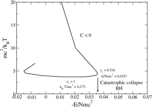
Figure 5: Series of equilibria (caloric curve) of heavily truncated Maxwell-Boltzmann distributions in general relativity (according to the data of Ipser ipser69b ). The series of equilibria is parametrized by the central redshift $z_{0}$. It has a snail-like (spiral) structure of which we only see the begining. The equilibrium states are all canonically unstable. In the microcanonical ensemble, only the part of the curve up to $z_{c}=0.516$ (corresponding to the turning point of binding energy) is stable. In this region the specific heat is negative. The onset of thermodynamical instability coincides with the onset of dynamical instability.

We can now investigate the dynamical and thermodynamical stability of the equilibrium states of relativistic star clusters in more detail. Let us first consider their thermodynamical stability. In a sense, we can say that Zel’dovich and Podurets zp considered the canonical ensemble (fixed $T_{\infty}$) while Ipser ipser69b considered the microcanonical ensemble (fixed $E$). The fact that they obtained different results is related to the notion of ensembles inequivalence for systems with long-range interactions like self-gravitating systems.

Let us first consider the microcanonical ensemble which is the rigorous statistical ensemble that we should use in order to describe isolated star clusters. Let us assume that the system is stable at sufficiently high energies (i.e. close to $0^{-}$). Using the Poincaré criterion poincare , we conclude that the system is microcanonically stable on the upper branch of Fig. 5 up to the first turning point of fractional binding energy and becomes unstable afterwards. We note that the system becomes microcanonically unstable when the specific heat becomes positive. This result was first stated by Horwitz and Katz hk .

Let us now turn to the canonical ensemble. If the system were stable at sufficiently low temperatures, using the Poincaré criterion poincare , we would conclude that the system is canonically stable up to the first turning point of temperature and becomes canonically unstable afterwards. However, considering the topology of the series of equilibria in Fig. 5, this is not possible. Indeed, we know from general arguments that canonical stability implies microcanonical stability aaantonov ; cc . Now, we note that the first turning point of temperature occurs after the first turning point of binding energy. Therefore, if the series of equilibria were canonically stable up to the first turning point of temperature it would also be microcanonically stable up to that point. But, we know that the series of equilibria becomes unstable after the first turning point of binding energy. Therefore, we arrive at a contradiction. Since a change of stability in the canonical ensemble can occur only at a turning point of temperature, we conclude that the whole series of equilibria is canonically unstable.

Let us finally consider the dynamical stability of the system with respect to a collisionless evolution described by the Vlasov-Einstein equations. We know from general arguments that thermodynamical stability implies dynamical stability ipser80 . From the previous results obtained in the microcanonical ensemble, we conclude that the system is both thermodynamically and dynamically stable up to the first turning point of fractional binding energy. This is a particular case (for isothermal systems) of the general binding energy criterion derived by Ipser ipser80 . After the first turning point of fractional binding energy the system is thermodynamically unstable. On the other hand, Ipser ipser69b has shown numerically that the system is also dynamically unstable after that point. This lead Ipser ipser80 to the conclusion that, in general relativity, dynamical and microcanonical thermodynamical stability coincide contrary to the case of Newtonian systems (see Appendix A.1).

From the previous results obtained in the canonical ensemble, we cannot conclude anything regarding the dynamical stability of collisionless isothermal star clusters since all equilibria are canonically unstable. However, we know that the canonical stability of a collisionless star cluster is equivalent to the dynamical stability of the corresponding barotropic star with respect to the Euler-Einstein equations roupas1 ; roupas1E ; gsw ; fhj . Therefore, our observation that all the equilibria of isothermal relativistic star clusters are canonically unstable is consistent with Ipser’s ipser69b finding that all the relativistic stars with the same equation of state as the isothermal star clusters are dynamically unstable.

The dynamical evolution of relativistic star clusters is reviewed in the Introduction (see also the introduction of acb ). Because of collisions between stars and evaporation, the system evolves quasi-statically along the series of equilibria. The natural evolution corresponds to an increase of the central density $\rho_{0}$ (or central redshift $z_{0}$) that parametrizes the series of equilibra. During the evolution, the energy decreases. On the other hand, the temperature decreases in the region of positive specific heat $C=dE/dT_{\infty}>0$ and increases in the region of negative specific heat $C=dE/dT_{\infty}<0$. At the turning point of energy (minimum energy state) the system becomes unstable and undergoes a gravitational collapse. This is a dynamical (and thermodynamical) instability of general relativistic origin taking place on a dynamical (short) timescale. It ultimately leads to the formation of a black hole surrounded by a halo of stars.

Appendix B Analogies and differences between box models and truncated distributions

B.1 Newtonian gravity

In Newtonian gravity, the series of equilibria of truncated isothermal distributions (see Fig. 4) is qualitatively similar to the series of equilibria of box-confined isothermal systems (see Fig. 2 and the “cold spiral” of Fig. 1). The main difference stems from the fact that, for open clusters, equilibrium states necessarily have a negative energy $E<0$. Indeed, when the energy is positive ($E>0$) the stars are unbounded and disperse away. If the system is confined within a box, equilibrium states with a positive energy are possible because the stars bounce off the wall. Apart from this difference, the series of equilibria in Figs. 2 and 4 have a similar spiralling shape. They display a turning point of temperature before the turning point of energy. For the two systems, equilibrium states are canonically stable up to the turning point of temperature and microcanonically stable up to the turning point of energy. We note that the dimensionless temperature and the dimensionless energy in the two models are related by

$$\eta=\sigma\beta mv_{0}^{2}\quad{\rm and}\quad\Lambda=-\frac{1}{\sigma}\frac{E}{Mv_{0}^{2}}\quad{\rm where}\quad\sigma=\frac{GM}{Rv_{0}^{2}}.$$ (159)

In practice $\sigma\sim 1$ since $v_{0}$ corresponds to the virial velocity of the cluster. We see that the orders of magnitude of the dimensionless energies and dimensionless temperatures in Figs. 2 and 4 are consistent with each other.

B.2 General relativity

We now turn to the general relativistic case. The values of $E$ and $T_{\infty}$ tabulated by Ipser ipser69b correspond to strongly relativistic stellar systems. Therefore, the caloric curve of Fig. 5 describes only the strongly relativistic part of the caloric curve (hot spiral). We need to complete this caloric curve with the nonrelativistic part from Fig. 4 (cold spiral). To that purpose, we first recall that, in the nonrelativistic regime, $\beta mv_{0}^{2}$ and ${E}/{Mv_{0}^{2}}$ are of the same order of magnitude as $\eta$ and $\Lambda$ in the box model (see Appendix B.1). On the other hand, in the relativistic regime, we have the relations

$$\eta=\nu\frac{mc^{2}}{k_{B}T_{\infty}},\quad{\rm and}\quad\Lambda=-\frac{1}{\nu}\frac{E}{Nmc^{2}}\quad{\rm where}\quad\nu=\frac{GNm}{Rc^{2}}.$$ (160)

As shown in Refs. roupas ; acb , the parameter $\nu$ belongs to the interval $[0,0.1764]$. In order to construct the complete caloric curve of truncated isothermal star clusters, we first determine the relativistic curve $\eta(\Lambda)$ from Fig. 5 by multiplying ${mc^{2}}/{k_{B}T_{\infty}}$ by $\nu$ and dividing ${E}/{Nmc^{2}}$ by $\nu$, then we add the nonrelativistic caloric curve of Fig. 4. We note that the result depends on the parameter $\nu$ so we actually have a family of caloric curves. For illustration, we have taken $\nu=0.015$. This leads to the complete caloric curve reported in Fig. 6. Our procedure is of course very approximate but it is sufficient to show the idea. It will be important in future works to improve this procedure and determine the family of caloric curves exactly.

From the complete caloric curve of Fig. 6 it is now easy to understand the thermodynamical stability/instability of isothermal clusters in both nonrelativistic and relativistic regimes. We again advocate the Poincaré turning point criterion poincare .

In the microcanonical ensemble, the nonrelativistic branch is stable up to the first fundamental turning point of energy MCE (see Appendix A.1). At that point the series of equilibria $\beta(-E)$ rotates clockwise so that a mode of stability is lost. A new mode of stability is lost at each subsequent turning point of energy where the series of equilibria rotates clockwise. At some point the series of equilibria unwinds and rotates anti-clockwise (the unwinding of the spiral is represented schematically by a dashed line in Fig. 6). A mode of stability is gained at each turning point of energy where the series of equilibria rotates anticlockwise. Finally, the series of equilibria on the relativistic branch becomes stable again (after rotating anticlockwise an even number of times) and remains stable until the second fundamental turning point of energy MCE’ at which it becomes unstable again. After that point the series of equilibria rotates only clockwise so that it remains unstable until the end. This is consistent with the results from Appendix A.2.

In the canonical ensemble, the nonrelativistic branch is stable up to the first turning point of temperature CE (see Appendix A.1). At that point the series of equilibria $\beta(-E)$ rotates clockwise so that a mode of stability is lost. The series of equilibria thus becomes unstable. It remains unstable until the end because it can never recover the first mode of stability that it has lost (it rotates anticlockwise an odd number of times). This is why we found in Appendix A.2 that the relativistic branch is always unstable in the canonical ensemble.

The caloric curve of Fig. 6 provides a nice illustration of the scenario discussed in the Introduction. Because of collisions and evaporation a Newtonian stellar system evolves along the upper branch of the series of equilibria. When it reaches the first fundamental turning point of energy it becomes thermodynamically unstable (while remaining dynamically stable) and undergoes a gravothermal catastrophe. It then evolves towards very hot and very dense configurations and becomes relativistic. It may then reach a stable relativistic isothermal equilibrium distribution. Again, because of collisions and evaporation, a relativistic star cluster evolves along the lower branch of the series of equilibria. When it reaches the second fundamental turning point of energy it becomes thermodynamically and dynamically unstable and undergoes a catastrophic collapse towards a black hole.

Figure 6: Complete caloric curve of truncated isothermal star clusters showing the nonrelativistic cold spiral and the relativistic hot spiral (for illustration we have taken $\nu=0.015$). The units of $\beta$ and $E$ are the same as in Fig. 4. Nonrelativistic clusters undergo a gravothermal catastrophe at MCE and become relativistic. They can then undergo a catastrophic collapse at MCE’ leading to the formation of a black hole.

We can now compare the caloric curve of truncated isothermal star clusters (see Fig. 6) with the caloric curve of box-confined isothermal systems (see Fig. 1). As we have seen in Appendix B.1, the nonrelativistic parts of the caloric curves are relatively similar. In particular, they present a “cold” spiral at negative energies. We now consider the relativistic parts of the caloric curves. In that case, a “hot” spiral arises because, in the ultrarelativistic limit (corresponding to very high energy densities), the equation of state of an isothermal gas is $P=\epsilon/3$ like for the self-gravitating black-body radiation. However, in the relativistic domain, the series of equilibria of truncated isothermal distributions (see Figs. 5 and 6) and the series of equilibria of box-confined isothermal systems (see Figs. 1 and 3) are very different.

(i) The origin of the difference stems from the fact that, for open clusters, stable equilibrium states necessarily have a negative energy $E<0$. By contrast, when the system is confined within a box, stable equilibrium states with a positive energy are allowed because of the pressure exerted by the box. For box-confined systems, the “hot spiral” appears at very large positive energies. At such energies, the relativistic isothermal gas behaves as a form of radiation confined within a cavity like in the studies of Sorkin et al. sorkin and Chavanis aarelat2 . There are no such equilibrium states with very large positive energies in open star clusters. In open star clusters, the “hot spiral” appears at energies (positive and negative) around $E=0$. In addition, the stable equilibrium states necessarily have a negative energy.

(ii) For box-confined isothermal systems the cold and hot spiral are quite distinct. The cold spiral appears at negative energies and the hot spiral appear at large positive energies. For open star clusters, the cold and hot spirals both appear at approximately the same range of (negative) energies. When general relativity is taken into account, the cold spiral of Fig. 4 unwinds and connects the hot spiral of Fig. 5 as sketched in Fig. 6.

As a result, a relativistic isothermal cluster in a box behaves very differently from a truncated relativistic isothermal cluster. This remark may question the physical relevance of the “hot spiral” at large energies for realistic isothermal star clusters except if one can justify a form of confinement playing the role of the box. This may be the case for relativistic stars. The box could be caused by a medium exerting a tremendously large pressure on an ultrarelativistic gas, like in the supernova phenomenon where the system achieves a “core-halo” structure. The core could correspond to the ultrarelativistic isothermal gas and the halo could play the role of the box. In that case, the core would be sustained by the external pressure of the halo. However, this scenario remains to be put on a more rigorous basis.

Appendix C Entropy and free energy as functionals of the density for nonrelativistic self-gravitating classical particles

We consider a nonrelativistic system of self-gravitating classical particles. The statistical equilibrium state is obtained by maximizing the Boltzmann entropy at fixed energy and particle number in the microcanonical ensemble, or by minimizing the free energy at fixed particle number in the canonical ensemble. In Appendix C.2 of Paper I, we have introduced entropy and free energy functionals of the distribution function $f({\bf r},{\bf v})$. In Sec. II.2 of this paper and in Appendix C.1.a of Paper I, we have introduced entropy and free energy functionals of the local density $n(r)$ and local kinetic energy $\epsilon_{\rm kin}(r)$. In this Appendix, we introduce entropy and free energy functionals of the local density $n(r)$.

C.1 Microcanonical ensemble

In the microcanonical ensemble, the statistical equilibrium state is obtained by maximizing the Boltzmann entropy $S[f]$ at fixed energy $E$ and particle number $N$. To solve this maximization problem, we proceed in two steps. We first maximize $S[f]$ at fixed $E$, $N$ and particle density $n(r)$. Since $n(r)$ determines the particle number $N[n]$ and the gravitational energy $W[n]$, this is equivalent to maximizing $S[f]$ at fixed kinetic energy $E_{\rm kin}[f]$ and particle density $n(r)$. The variational problem for the first variations (extremization) can be written as

$$\frac{\delta S}{k_{B}}-\beta\delta E_{\rm kin}+\int\alpha(r)\delta n\,d{\bf r}=0,$$ (161)

where $\beta$ is a global (uniform) Lagrange multiplier and $\alpha(r)$ is a local (position dependent) Lagrange multiplier. This variational problem yields

$$f({\bf r},{\bf p})=\frac{g}{h^{3}}e^{-\beta p^{2}/2m+\alpha(r)}.$$ (162)

As in Appendix C1 of Paper I, we can show that this distribution is the global maximum of $S[f]$ at fixed $E_{\rm kin}[f]$ and $n(r)$. Substituting Eq. (162) into Eqs. (I-17), (I-18) and (I-20), we get

$$n(r)=\frac{g}{h^{3}}(2\pi mk_{B}T)^{3/2}e^{\alpha(r)},$$ (163)

$$\epsilon_{\rm kin}(r)=\frac{3}{2}n(r)k_{B}T,$$ (164)

$$P(r)=\frac{2}{3}\epsilon_{\rm kin}(r)=n(r)k_{B}T.$$ (165)

The Lagrange multiplier $\alpha(r)$ is determined by the density $n(r)$ according to Eq. (163). As a result, the distribution function (162) can be written in terms of the density as

$$f({\bf r},{\bf p})=n({r})\left(\frac{\beta}{2\pi m}\right)^{3/2}e^{-\beta{p}^{2}/2m}.$$ (166)

On the other hand, since $T$ is uniform, we see from Eq. (165) that the equation of state is isothermal: $P(r)=n(r)k_{B}T$. The temperature $T$ is determined by the kinetic energy $E_{\rm kin}[n(r),T]=E-W[n(r)]$ using Eq. (164) integrated over the volume giving $E_{\rm kin}=(3/2)Nk_{B}T$. In other words, the temperature is determined by the energy constraint

$$E=\frac{3}{2}Nk_{B}T+W[n(r)].$$ (167)

We note that $T$ is a functional of the density $n(r)$ but, for brevity, we shall not write this dependence explicitly. Substituting the Maxwell-Boltzmann distribution (166) into the entropy density (1) we obtain

$$\frac{s(r)}{k_{B}}=\frac{5}{2}n(r)-n(r)\ln n(r)-n(r)\ln\left(\frac{h^{3}}{g}\right)+\frac{3}{2}n(r)\ln(2\pi mk_{B}T),$$ (168)

which is equivalent to the integrated Gibbs-Duhem relation (7). The entropy is given by

$$\frac{S}{k_{B}}=\frac{5}{2}N-\int n(r)\ln n(r)\,4\pi r^{2}\,dr-N\ln\left(\frac{h^{3}}{g}\right)+\frac{3}{2}N\ln(2\pi mk_{B}T).$$ (169)

Finally, the statistical equilibrium state in the microcanonical ensemble is obtained by maximizing the entropy $S[n(r),T]$ at fixed particle number $N$, the energy constraint being taken into account in the determination of the temperature $T[n]$ through Eq. (167). The variational problem for the first variations (extremization) can be written as

$$\frac{\delta S}{k_{B}}+\alpha_{0}\delta N=0.$$ (170)

The conservation of energy implies [see Eq. (167)]:

$$0=\delta E_{\rm kin}+\int m\Phi\delta n\,d{\bf r}.$$ (171)

Using Eqs. (161) and (171), and proceeding as in Appendix F1 of Paper I, or performing the variations over $\delta n$ and $\delta T$ directly on the explicit expressions (167) and (169) we obtain

$$\alpha(r)=\alpha_{0}-\beta m\Phi(r)\qquad{\rm or}\qquad n(r)=\frac{g}{h^{3}}(2\pi mk_{B}T)^{3/2}e^{\alpha_{0}-\beta m\Phi(r)}.$$ (172)

We then recover all the results of Sec. II. The interest of this formulation it that it allows us to solve more easily the stability problem related to the sign of the second variations of entropy. This problem has been studied in detail in paddyapj ; paddy ; sc . It has also been studied in aarelat1 within the framework of special relativity.

C.2 Canonical ensemble

In the canonical ensemble, the statistical equilibrium state is obtained by minimizing the Boltzmann free energy $F[f]=E[f]-TS[f]$ at fixed particle number $N$, or equivalently, by maximizing the Massieu function $J[f]=S[f]/k_{B}-\beta E[f]$ at fixed particle number $N$. To solve this maximization problem, we proceed in two steps. We first maximize $J[f]=S[f]/k_{B}-\beta E[f]$ at fixed $N$ and particle density $n(r)$. Since $n(r)$ determines the particle number $N[n]$ and the gravitational energy $W[n]$, this is equivalent to maximizing $S[f]/k_{B}-\beta E_{\rm kin}[f]$ at fixed particle density $n(r)$. The variational problem for the first variations (extremization) can be written as

$$\delta\left(\frac{S}{k_{B}}-\beta E_{\rm kin}\right)+\int\alpha(r)\delta n\,d{\bf r}=0,$$ (173)

where $\alpha(r)$ is a local (position dependent) Lagrange multiplier. Since $\beta$ is constant in the canonical ensemble, this is equivalent to the condition (161) yielding the distribution function (162). This distribution is the global maximum of $S[f]/k_{B}-\beta E_{\rm kin}[f]$ at fixed $n(r)$. We then obtain the same results as in Appendix C.1, except that $T$ is fixed while it was previously determined by the conservation of energy.

We can now simplify the expression of the free energy. The entropy is given by Eq. (169) and the energy by Eq. (167). Since $F=E-TS$, we obtain

$$F=W[n(r)]-Nk_{B}T+k_{B}T\int n(r)\ln n(r)\,4\pi r^{2}\,dr+Nk_{B}T\ln\left(\frac{h^{3}}{g}\right)-\frac{3}{2}Nk_{B}T\ln(2\pi mk_{B}T).$$ (174)

Using the foregoing results, the free energy can be written as a functional of the density as

$$F[n(r)]=U[n(r)]+W[n(r)],$$ (175)

where $U[n(r)]$ is the internal energy given by

$$U[n(r)]=-Nk_{B}T+k_{B}T\int n(r)\ln n(r)\,4\pi r^{2}\,dr+Nk_{B}T\ln\left(\frac{h^{3}}{g}\right)-\frac{3}{2}Nk_{B}T\ln(2\pi mk_{B}T).$$ (176)

Finally, the statistical equilibrium state in the canonical ensemble is obtained by minimizing the free energy $F[n]$ at fixed particle number $N$. The variational problem for the first variations (extremization) can be written as

$$\delta J+\alpha_{0}\delta N=0.$$ (177)

Decomposing the Massieu function as $J[f]=S[f]/k_{B}-\beta E_{\rm kin}[f]-\beta W[n]$ and proceeding as in Appendix F2 of Paper I, or performing the variations over $\delta n$ directly on the explicit expression (174) of the free energy we get

$$\alpha(r)=\alpha_{0}-\beta m\Phi(r)\qquad{\rm or}\qquad n(r)=\frac{g}{h^{3}}(2\pi mk_{B}T)^{3/2}e^{\alpha_{0}-\beta m\Phi(r)}.$$ (178)

We then recover all the results of Sec. II. The interest of this formulation it that it allows us to solve more easily the stability problem related to the sign of the second variations of free energy. This problem has been studied in detail in aaiso ; sc . It has also been studied in aarelat1 within the framework of special relativity.

Remark: We note that the free energy $F[\rho]$ coincides with the energy functional associated with the Euler-Poisson equations describing a gas with an isothermal equation of state $P=\rho k_{B}T/m$ (see Appendix G1 of Paper I). As a result, the thermodynamical stability of a classical self-gravitating system in the canonical ensemble is equivalent to the dynamical stability of the corresponding isothermal gas described by the Euler-Poisson equations aaiso . This is a particular case of the general result established in aaantonov which is valid for an arbitrary form of entropy. According to the Poincaré turning point criterion, the series of equilibria becomes both thermodynamically unstable (in the canonical ensemble) and dynamically unstable with respect to the Euler-Poisson equations at the first turning point of temperature (or, equivalently, at the first turning point of mass).

References

- (1) P.H. Chavanis, preprint (Paper I)
- (2) R.C. Tolman, Phys. Rev. 35, 904 (1930)
- (3) W.J. Cocke, Ann. I.H.P. 4, 283 (1965)
- (4) G. Horwitz, J. Katz, Ann. Phys. (USA) 76, 301 (1973)
- (5) J. Katz, G. Horwitz, Astrophys. J. 194, 439 (1974)
- (6) J. Katz, G. Horwitz, M. Klapisch, Astrophys. J. 199, 307 (1975)
- (7) J. Katz, Y. Manor, Phys. Rev. D 12, 956 (1975)
- (8) J. Katz, G. Horwitz, Astrophys. J. 33, 251 (1977)
- (9) G. Horwitz, J. Katz, Astrophys. J. 223, 311 (1978)
- (10) J.R. Ipser, Astrophys. J. 238, 1101 (1980)
- (11) R.D. Sorkin, R.M. Wald, Z.Z. Jiu, Gen. Relat. Grav. 13, 1127 (1981)
- (12) W.M. Suen, K. Young, Phys. Rev. A 35, 406 (1987)
- (13) W.M. Suen, K. Young, Phys. Rev. A 35, 411 (1987)
- (14) N. Bilic, R.D. Viollier, Gen. Relat. Grav. 31, 1105 (1999)
- (15) P.H. Chavanis, Astron. Astrophys. 381, 709 (2002)
- (16) P.H. Chavanis, Astron. Astrophys. 483, 673 (2008)
- (17) S. Gao, Phys. Rev. D 84, 104023 (2011)
- (18) S. Gao, Phys. Rev. D 85, 027503 (2012)
- (19) Z. Roupas, Class. Quantum Grav. 30, 115018 (2013)
- (20) S.R. Green, J.S. Schiffrin, R.M. Wald, Class. Quantum Grav. 31, 035023 (2014)
- (21) X. Fang, S. Gao, Phys. Rev. D 90, 044013 (2014)
- (22) Z. Roupas, Class. Quantum Grav. 32, 119501 (2015)
- (23) J.S. Schiffrin, Class. Quantum Grav. 32, 185011 (2015)
- (24) K. Prabhu, J.S. Schiffrin, R.M. Wald, Class. Quantum Grav. 33, 185007 (2016)
- (25) X. Fang, X. He, J. Jing, Eur. Phys. J. C 77, 893 (2017)
- (26) J.R. Oppenheimer, G.M. Volkoff, Phys. Rev. 55, 374 (1939)
- (27) O. Klein, Rev. Mod. Phys. 21, 531 (1949)
- (28) G. Alberti, P.H. Chavanis, arXiv:1808.01007
- (29) G. Alberti, P.H. Chavanis, arXiv:1908.10316
- (30) P.H. Chavanis, M. Lemou, F. Méhats, Phys. Rev. D 91, 063531 (2015)
- (31) S. Chandrasekhar, Principles of Stellar Dynamics (University of Chicago Press, 1942)
- (32) V.A. Ambartsumian, Ann. Leningrad State Univ. 22, 19 (1938)
- (33) L. Spitzer, MNRAS 100, 396 (1940)
- (34) R. Woolley, MNRAS 114, 191 (1954)
- (35) I. King, Astron. J. 71, 64 (1966)
- (36) A.S. Eddington, MNRAS 76, 572 (1916)
- (37) R.W. Michie, MNRAS 125, 127 (1963)
- (38) D. Lynden-Bell, R. Wood, Mon. Not. R. Astron. Soc. 138, 495 (1968)
- (39) J. Katz, MNRAS 190, 497 (1980)
- (40) V.A. Antonov, Vest. Leningr. Gos. Univ. 7, 135 (1962)
- (41) R.B. Larson, Mon. Not. R. Astron. Soc. 147, 323 (1970)
- (42) R.B. Larson, Mon. Not. R. Astron. Soc. 150, 93 (1970)
- (43) M. Hénon, Astrophys. Space Sci. 13, 284 (1971)
- (44) I. Hachisu, Y. Nakada, K. Nomoto, D. Sugimoto, Prog. Theor. Phys. 60, 393 (1978)
- (45) D. Lynden-Bell, P.P. Eggleton, Mon. Not. R. Astron. Soc. 191, 483 (1980)
- (46) H. Cohn, Astrophys. J. 242, 765 (1980)
- (47) S. Inagaki, D. Lynden-Bell, Mon. Not. R. Astron. Soc. 205, 913 (1983)
- (48) D. Sugimoto, E. Bettwieser, Mon. Not. R. Astron. Soc. 204, 19 (1983)
- (49) D. Heggie, N. Ramamani, Mon. Not. R. Astron. Soc. 237, 757 (1989)
- (50) J.P. Doremus, M.R. Feix, G. Baumann, Phys. Rev. Lett. 26, 725 (1971)
- (51) J.P. Doremus, M.R. Feix, G. Baumann, Astron. Astrophys. 29, 401 (1973)
- (52) D. Gillon, M. Cantus, J.P. Doremus, G. Baumann, Astron. Astrophys. 50, 467 (1976)
- (53) J.F. Sygnet, G. Des Forets, M. Lachieze-Rey, R. Pellat, Astrophys. J. 276, 737 (1984)
- (54) H. Kandrup, J.F. Sygnet, Astrophys. J. 298, 27 (1985)
- (55) H. Kandrup, Astrophys. J. 370, 312 (1991)
- (56) Y.B. Zel’dovich, M.A. Podurets, Soviet Astron. – AJ 9, 742 (1966)
- (57) E.D. Fackerell, Ph.D. thesis, University of Sydney (1966)
- (58) E. Fackerell, Astrophys. J. 153, 643 (1968)
- (59) J.R. Ipser, K.S. Thorne, Astrophys. J. 154, 251 (1968)
- (60) J.R. Ipser, Astrophys. J. 156, 509 (1969)
- (61) J.R. Ipser, Astrophys. J. 158, 17 (1969)
- (62) E. Fackerell, Astrophys. J. 160, 859 (1970)
- (63) A.W. Sudbury, Mon. Not. R. Astron. Soc. 147, 187 (1970)
- (64) K. Suffern, E. Fackerell, Astrophys. J. 203, 477 (1976)
- (65) E. Fackerell, K. Suffern, Aust. J. Phys. 29, 311 (1976)
- (66) M. Merafina, R. Ruffini, Astron. Astrophys. 221, 4 (1989)
- (67) M. Merafina, R. Ruffini, Europhys. Lett. 9, 621 (1989)
- (68) M. Merafina, R. Ruffini, Astron. Astrophys. 227, 415 (1990)
- (69) G.S. Bisnovatyi-Kogan, M. Merafina, R. Ruffini, E. Vesperini, Astrophys. J. 414, 187 (1993)
- (70) G.S. Bisnovatyi-Kogan, M. Merafina, R. Ruffini, E. Vesperini, Astrophys. J. 500, 217 (1998)
- (71) H. Poincaré, Acta Math. 7, 259 (1885)
- (72) D. Fackerell, J. Ipser, K. Thorne, Comments Ap. and Space Phys. 1, 134 (1969)
- (73) S.L. Shapiro, S.A. Teukolsky, Astrophys. J. 298, 34 (1985)
- (74) S.L. Shapiro, S.A. Teukolsky, Astrophys. J. 298, 58 (1985)
- (75) S.L. Shapiro, S.A. Teukolsky, Astrophys. J. 292, L41 (1985)
- (76) S.L. Shapiro, S.A. Teukolsky, Astrophys. J. 307, 575 (1986)
- (77) C.S. Kochanek, S.L. Shapiro, S.A. Teukolsky, Astrophys. J. 320, 73 (1987)
- (78) F. Rasio, S.L. Shapiro, S.A. Teukolsky, Astrophys. J. 344, 146 (1989)
- (79) S.L. Shapiro, S.A. Teukolsky, Phil. Trans. R. Soc. Lond. A 340, 365 (1992)
- (80) S.L. Shapiro, S.A. Teukolsky, Astrophys. J. 234, L177 (1979)
- (81) S.L. Shapiro, S.A. Teukolsky, Astrophys. J. 235, 199 (1980)
- (82) F. Hoyle, W.A. Fowler, Nature 213, 373 (1967)
- (83) F. Hoyle, W.A. Fowler, Mon. Not. R. Astron. Soc. 125, 169 (1963)
- (84) F. Hoyle, W.A. Fowler, Nature 197, 533 (1963)
- (85) H.S. Zapolsky, Astrophys. J. 153, L163 (1968)
- (86) E.E. Salpeter, Astrophys. J. 140, 796 (1964)
- (87) Ya.B. Zel’dovich, Soviet Phys. Doklady 9, 195 (1964)
- (88) G.S. Bisnovatyi-Kogan, Ya. B. Zel’dovich, Astrofizika 5, 223 (1969)
- (89) G.S. Bisnovatyi-Kogan, K.S. Thorne, Astrophys. J. 160, 875 (1970)
- (90) F. Rasio, S.L. Shapiro, S.A. Teukolsky, Astrophys. J. 336, L63 (1989)
- (91) M. Merafina, R. Ruffini, Astrophys. J. 454, L89 (1995)
- (92) S. Balberg, S.L. Shapiro, S. Inagaki, Astrophys. J. 568, 475 (2002)
- (93) S. Balberg, S.L. Shapiro, Phys. Rev. Lett. 88, 101301 (2002)
- (94) J. Pollack, D. Spergel, P. Steinhardt, Astrophys. J. 804, 131 (2015)
- (95) P.H. Chavanis, M. Lemou, F. Méhats, Phys. Rev. D 92, 123527 (2015)
- (96) P.H. Chavanis, arXiv:1810.08948
- (97) J.R. Ipser, Astrophys. J. 193, 463 (1974)
- (98) L. Taff, H. van Horn, Astrophys. J. 197, L23 (1975)
- (99) G. Horwitz, J. Katz, Astrophys. J. 211, 226 (1977)
- (100) Y. Nakada, Publ. Astron. Soc. Japan 30, 57 (1978)
- (101) I. Hachisu, D. Sugimoto, Prog. Theor. Phys. 60, 123 (1978)
- (102) G. Horwitz, J. Katz, Astrophys. J. 222, 941 (1978)
- (103) J. Katz, Mon. Not. R. Astron. Soc. 183, 765 (1978)
- (104) J.R. Ipser, G. Horwitz, Astrophys. J. 232, 863 (1979)
- (105) S. Inagaki, Publ. Astron. Soc. Japan 32, 213 (1980)
- (106) M. Lecar, J. Katz, Astrophys. J. 243, 983 (1981)
- (107) J. Messer, H. Spohn, J. Stat. Phys. 29, 561 (1982)
- (108) J.F. Luciani, R. Pellat, Astrophys. J. 317, 241 (1987)
- (109) M. Kiessling, J. Stat. Phys. 55, 203 (1989)
- (110) T. Padmanabhan, Astrophys. J. Supp. 71, 651 (1989)
- (111) T. Padmanabhan, Phys. Rep. 188, 285 (1990)
- (112) H.J. de Vega, N. Sanchez, F. Combes, Phys. Rev. D 54, 6008 (1996)
- (113) B. Semelin, H.J. de Vega, N. Sanchez, F. Combes, Phys. Rev. D 59, 125021 (1999)
- (114) J. Katz, I. Okamoto, MNRAS 317, 163 (2000)
- (115) B. Semelin, N. Sanchez, H.J. de Vega, Phys. Rev. D 63, 084005 (2001)
- (116) H.J. de Vega, N. Sanchez, Nucl. Phys. B 625, 409 (2002)
- (117) H.J. de Vega, N. Sanchez, Nucl. Phys. B 625, 460 (2002)
- (118) P.H. Chavanis, Astron. Astrophys. 381, 340 (2002)
- (119) P.H. Chavanis, C. Rosier, C. Sire, Phys. Rev. E 66, 036105 (2002)
- (120) C. Sire, P.H. Chavanis, Phys. Rev. E 66, 046133 (2002)
- (121) P.H. Chavanis, Astron. Astrophys. 401, 15 (2003)
- (122) J. Katz, Found. Phys. 33, 223 (2003)
- (123) P.H. Chavanis, Astron. Astrophys. 432, 117 (2005)
- (124) P.H. Chavanis, Int. J. Mod. Phys. B 20, 3113 (2006)
- (125) M. Sormani, G. Bertin, Astron. Astrophys. 552, A37 (2013)
- (126) Z. Roupas, Class. Quantum Grav. 32, 135023 (2015)
- (127) C. Sire, P.H. Chavanis, Phys. Rev. E 69, 066109 (2004)
- (128) F. Juttner, Ann. Phys. 339, 856 (1911)
- (129) F. Juttner, Ann. Phys. 340, 145 (1911)
- (130) M. Planck, Ann. Phys. 26, 1 (1908)
- (131) P.H. Chavanis, Astron. Astrophys. 451, 109 (2006)
- (132) A. Campa, P.H. Chavanis, J. Stat. Mech. 06, 06001 (2010)
- (133) S. Chandrasekhar, in General Relativity, papers in honour of J.L. Synge, Edited by L.O’ Raifeartaigh (Oxford, 1972)
- (134) P.H. Chavanis, Phys. Rev. E 65, 056123 (2002)
- (135) N.A. Dmitriev, S.A. Kholin, Voprosy kosmogonii 9, 254 (1963)
- (136) Ya.B. Zel’dovich, Soviet Phys. JETP 15, 1158 (1962)