Non-monotonic response of a sheared magnetic liquid crystal to an external field

Abstract

Utilizing molecular dynamics simulations, we report a non-monotonic dependence of the shear stress on the strength of an external magnetic field ($H$) in a liquid-crystalline mixture of magnetic and non-magnetic anisotropic particles. This non-monotonic behavior is in sharp contrast with the well-studied monotonic $H$-dependency of the shear stress in conventional ferrofluids, where the shear stress increases with $H$ until it reaches a saturation value. We relate the origin of this non-monotonicity to the competing effects of particle alignment along the shear-induced direction, on the one hand, and the magnetic field direction, on the other hand. To isolate the role of these competing effects, we consider a two-component mixture composed of particles with effectively identical steric interactions, where the orientations of a small fraction, i.e. the magnetic ones, are coupled to the external magnetic field. By increasing $H$ from zero, the orientations of the magnetic particles show a Fréederickz-like transition and eventually start deviating from the shear-induced orientation, leading to an increase in shear stress. Upon further increase of $H$, a demixing of the magnetic particles from the non-magnetic ones occurs which leads to a drop in shear stress, hence creating a non-monotonic response to $H$. Unlike the equilibrium demixing phenomena reported in previous studies, the demixing observed here is neither due to size-polydispersity nor due to a wall-induced nematic transition. Based on a simplified Onsager analysis, we rather argue that it occurs solely due to packing entropy of particles with different shear- or magnetic-field-induced orientations.

I Introduction

As proposed in a seminal work brochard1970theory by Brochard and de Gennes, doping liquid crystals (LC) with magnetic nano-particles (MNP) leads to remarkable hybrid materials whose properties can be controlled by an external magnetic field. These stimuli-responsive materials exhibit rich self-assembly in equilibrium and show marked effects under external fields rault1970ferronematics ; mertelj2013ferromagnetism ; mertelj2014magneto ; liu2016biaxial ; podoliak2012magnetite ; kopvcansky2008structural . A key factor in determining these emergent properties is the shape of the MNPs kopvcansky2008structural ; peroukidis2015tunable ; peroukidis2015spontaneous : Commonly, the MNPs are either spherical (and hence different from the LCs), or they are anisotropic with a large size disparity between the MNPs and LC particles  chen1983observation ; kopvcansky2008structural ; kyrylyuk2011controlling ; podoliak2012magnetite . In this paper, we investigate, on a computational basis, mixtures where the MNPs are identical to LCs in their anisotropy and size. This is a timely issue due to recent advances in experimental realizations of such anisotropic magnetic particles buluy2011magnetic ; mertelj2013ferromagnetism ; martinez2016dipolar ; kredentser2017magneto , which has motivated also a number of analytical and numerical studies sebastian2018director ; potisk2018magneto ; zarubin2018ferronematic ; zarubin2018effective .

The aforementioned studies sebastian2018director ; potisk2018magneto ; zarubin2018ferronematic ; zarubin2018effective focus on the effect of the magnetic field on the structural and optical properties. Here, we focus on a different aspect of the response to the external field, that is, the mechanical response of the mixture. A key difference between optical and mechanical responses is that, unlike in the optical case where light is transmitted through the sample without changing the structure, a mechanical perturbation itself can lead to structural changes. In particular, when the system is sheared, this leads to shear-induced changes of the structure blaak2004homogeneous ; ripoll2008attractive ; mokshin2008shear ; mandal2012heterogeneous ; shrivastav2016heterogeneous . We show that these shear-induced effects combined with the effects of the magnetic field induced effects lead to an intriguing mechanical response and structural changes.

A focus of the present study is to isolate the role of the magnetic field-induced orientation of the MNPs on the structure and rheology of such mixtures. To achieve this goal, we consider a mixture where not only the shape and size of the MNPs and LCs are identical, but also they interact via the same interparticular potential. Only the directions of the MNPs are coupled to the external magnetic field, and this coupling distinguishes the MNPs from the LCs. The assumed monodispersity in size and uniformity in inter-particular interaction has several consequences: (i) there is no specific anchoring between the LCs and MNPs beyond anchoring among LCs and MNPs, (ii) polydispersity-induced phenomena, which are by themselves subject of intensive research kikuchi2007mobile ; zaccarelli2015polydispersity ; heckendorf2017size ; ferreiro2016spinodal ; verhoeff2009liquid ; speranza2002simplified , are absent here, and (iii) unlike Refs. alvarez2012percolation ; schmidle2012phase ; sreekumari2013slow ; may2016colloidal ; peroukidis2016orientational ; shrivastav2019anomalous , there is no structure formation due to the direct magnetic dipole-dipole interaction between the MNPs. These properties of our model enable us to isolate the role of the selectively controlled direction of particles and study its effect on the structure and rheology of the whole system.

In pure ferrofluids, the interplay of an external magnetic field and shear leads to the well-known magnetoviscous effects (see Ref. odenbach2004recent and references therein): By applying the magnetic field, the viscosity of the system strongly and monotonically increases. This monotonic increase appears even for very dilute systems, where the dipole-dipole interactions are negligible rosensweig1969viscosity ; hall1969viscosity ; shliomis1971effective . However, for mixtures containing anisotropic MNPs, such effects are not studied, to the best of our knowledge. Our results show that the shear stress, and thus the viscosity, displays an intriguing non-monotonic dependence on the strength of the magnetic field. We analyze this shear-stress behavior by investigating its correlation to the structure of the mixture at different magnetic field values.

From methodological point of view, we use extensive nonequilibrium molecular dynamics (NEMD) simulations. Although NEMD simulations, in practice, have restrictions regarding accessible time and length scales, they nevertheless enable us to study the mixture in the presence of both shear and external magnetic field, where an analytical approach is missing. Furthermore, in NEMD simulations, no assumption on the spatial distribution of the particles is imposed, contrary to studies sebastian2018director ; potisk2018magneto which are based on continuum theories. In these continuum models, a homogeneous distribution of MNPs is assumed. Our results show that such an assumption is, in fact, not fulfilled. Indeed, we find clear evidence for the formation of an inhomogeneous spatial distribution with pronounced consequences for the mechanical response of the system.

In resemblance to the geometry of a rheometer, we shear the mixture by relative motion of two walls, and obtain the shear stress directly measuring the exerted forces on the walls. To analyze the structure of the sample, we use well-established quantities characterizing the orientational order, and also introduce a new quantity to characterize the positional distribution of MNPs across the system. Using these quantities, we argue that the non-monotonic behavior of the stress emerges as a delicate interplay between (i) an increase in stress due to orientational deviations of the MNPs from the shear-induced orientation, and (ii) a decrease in stress due to an entropic demixing, which is caused by differences of the orientations of the LCs and MNPs.

II Simulation setup

The simulation setup consists of ellipsoidal uniaxial Gay-Berne (GB) particles berardi1998gay , where a fraction of them has a permanent magnetic point dipole embedded in the particle center and pointing along the long axis. The system is subjected to (i) shear flow, which is realized via a relative motion of two walls between which the particles are confined, and (ii) an external magnetic field. In this section, after briefly introducing the GB parameters, the protocols for creating independent samples, shearing, and applying the external field are explained. Further, the observables and the relevant dimensionless parameters are introduced. A snapshot of the system, in the isotropic state, and in absence of the shear flow and magnetic field, is shown in Fig. 1.

For the GB potential, we adopt the notation and parameter values used in Ref. shrivastav2019anomalous . Similar to Ref. shrivastav2019anomalous the simulation units are set such that characteristic length and energy of the GB interaction, as well as particle mass are $\sigma_{0}=1$ and $\epsilon_{0}=1$, $m=1$, respectively. In these units, the lengths associated with semi-axes of the ellipsoids are $\sigma_{s}=1$ and $\sigma_{l}=3$ , for the short and the long axis of the ellipsoid, respectively. In addition to the GB interaction, the magnetic ellipsoids also interact via magnetic dipole-dipole potential. In the present work, however, we are primarily interested in the effect of the interaction of the magnetic dipoles with the external field. Therefore, the dipole-dipole interactions is set to a negligible value compared to the thermal energy. Thus, under the present conditions, thermal fluctuations are dominant in the sense that they prevent formation of structures due to the magnetic dipole-dipole interaction.

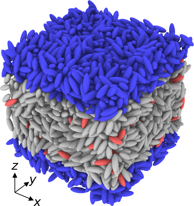
Figure 1: A snapshot of the simulation setup in absence of the shear and the external magnetic field: red, gray, and blue ellipsoidal particles represent magnetic, non-magnetic, and wall particles, respectively. The sample is in an isotropic state ($T=5$), the state from which the walls are created.

The protocol to create systems similar to Fig. 1 consists of two steps: (i) independent three-dimensional configurations are created by sampling from a molecular dynamics simulation with periodic boundary conditions at high temperature, (ii) walls are created via sudden freezing of two slabs of particles. These two steps are now explained detail.

As a first step, independent samples are created. For this purpose, an equilibrium molecular dynamics (EMD) simulation is performed with a constant number of particles, $N=4000$, at a constant volume (a cubic box with the spatial extension $L\simeq 23$), at a constant temperature, $T$. This simulation is performed with the LAMMPS plimpton1995fast package, where a new fix is introduced for embedding the point dipole moments along the longest axes of the magnetic particles. We set the number of magnetic particles to $N_{\mathrm{MNP}}=200$. Newton’s equation of motion for both rotational and positional degrees of freedom are integrated using the velocity-Verlet algorithm verlet1967computer ; swope1982computer with time-step $\delta t=5\times 10^{-3}$. The temperature is kept constant using a Langevin thermostat with the same parameters as in Ref. shrivastav2019anomalous .

For the present choice of GB parameters and the number density, the equilibrium system exhibits isotropic, nematic, and smectic phases brown1998effects . For the purpose of creating independent samples, we consider the case that the equilibrium system (in the absence of shear and the magnetic field) is deep in the isotropic state. We thus set the temperature to $T=5$, which is significantly larger than the isotropic-nematic transition temperature, $T_{\mathrm{IN}}\simeq 1.5$ brown1998effects . To assure the independence of the configurations, the time interval between each two consecutive samplings is chosen large enough such that, on average, particles move almost $10$ length units in that time interval.

In a second step, we create walls for each sample for the later implementation of shear flow (see Refs. siboni2013maintaining ; varnik2003shear ; hassani2018wall for a similar strategy). To this end, the sampling at high temperature is followed by a sudden quench of the upper and lower slabs of particles (relative to the $z$-direction), as depicted in Fig. 1 by blue-colored ellipsoids. The MNPs frozen in the walls are replaced with the LCs, such that the walls are solely composed of nonmagnetic particles. The thickness of the walls is chosen to be larger than the GB potential cutoff in our simulation setup. These frozen slabs serve as solid, impenetrable, and rough walls. Furthermore, as shown in Appendix A in Fig. 9, the roughness is large enough that the velocity profile obtained under shear does not show slip.

After creating walls, the system is quenched to the desired temperature and sheared by a relative motion of the walls along the $x$-direction with a constant velocity, yielding a time-independent global shear rate, $\dot{\Gamma}=\Delta V_{w}/L$, where $\Delta V_{w}$ is the difference in the velocities of the two wall. One should note, the Langevin thermostat is decoupled from particle’s $x$-coordinate to avoid the flow induced effects caused by shearing along this direction evans1986shear . This is a common practice to employ thermostating algorithms for sheared systems thompson1989simulations ; thompson1990shear ; soddemann2003dissipative ; zhou2005dynamic ; varnik2006structural ; niavarani2008slip ; bolintineanu2012no .

We now turn to the main physical quantities of interest in our study. Most important for the mechanical response is the shear stress. We calculate this quantity directly via summation of the $x$-component of the forces exerted by the liquid particles on the upper or lower wall particles, respectively,

$$\sigma_{xz}=\frac{1}{L^{2}}\sum_{i\in\mathrm{wall}}\sum_{j\in\mathrm{fluid}}\mathbf{f}_{ij,x}~{}.$$ (1)

In Eq. 1, $\mathbf{f}_{ij,x}$ is the $x$-component of the force on particle $i$ due to particle $j$, the summation over $i$ is restricted to particles composing the upper or lower wall, and the $j$ index runs over all fluid particles. We note that by using this method of $\sigma_{xz}$ calculation, we are not relying on the assumptions behind the virial expression for pressure tensor calculation such as homogeneity (as discussed in  cheung1991atomic ; todd1995pressure ), or being in equilibrium Schwabl2006 . Knowing the shear stress, we can calculate the apparent viscosity leslie1968some via $\eta_{a}:=\sigma_{xz}/\dot{\Gamma}$ . In this study, as we keep the shear rate constant, the qualitative behaviors of the shear stress and the apparent viscosity are identical. The ensemble averages of the stress and other quantities presented here are obtained by averaging over between $15$ to $50$ independent samples.

To characterize the orientational structure of the system, we measure the tensorial order parameter,

$$\mathbf{Q}_{\alpha}=\frac{1}{N_{\alpha}}\sum_{i=1}^{N_{\alpha}}\frac{1}{2}(3\hat{\mathbf{u}}_{\alpha,i}\otimes\hat{\mathbf{u}}_{\alpha,i}-{\mathbb{I}})~{},$$ (2)

where $\alpha\in\{\mathrm{LC,MNP}\}$ denotes the type of the particles, $N_{\alpha}$ is the corresponding number of particles, $\hat{\mathbf{u}}_{\alpha,i}$ is the unit vector along the longest axis of the $i$-th particle of type $\alpha$, and ${\mathbb{I}}$ denotes the second-rank unit tensor. The nematic order parameter, $S_{\alpha}$, and the direction associated with the nematic order director, $\hat{\mathbf{n}}_{\alpha}$, are obtained as the largest eigenvalue and the corresponding eigenvector of $\mathbf{Q}_{\alpha}$. The nematic order parameter changes in the range $[0,1]$, where $0$ corresponds to a completely random and isotropic state, and $1$ corresponds to perfect alignment of all particles. The critical value of $S$, i.e. the value at which isotopic-to-nematic transition occurs, is $S_{c}\simeq 0.43$, based on Maier-Saupe mean-field theory maier1958einfache ; maier1959einfache ; maier1960einfache .

We also measure the (particle) averaged polar order parameter, $P$, whose instantaneous value is given by

$$P=\frac{\mu}{N_{\mathrm{MNP}}}\sum_{i}^{N_{\mathrm{MNP}}}\hat{\mathbf{u}}_{\mathrm{MNP},i}~{}.~{}\hat{\mathbf{n}}_{\mathrm{MNP}}~{},$$ (3)

where the summation is limited only to the MNPs, and $\mu$ is the dipole moment of each MNP.

In order to obtain quantitative information on the instantaneous spatial distribution of MNPs and LCs, we measure the number density profile $\rho_{\alpha}(z_{0}):=n_{\alpha}(z_{0}-\delta z/2,z_{0}+\delta z/2)/(L^{2}\delta z)$ of particle type $\alpha$, where $n_{\alpha}$ is the instantaneous number of those particles between planes $z=z_{0}-\delta z/2$ and $z=z_{0}+\delta z/2$, and $\delta z=0.25$ is the discretization resolution along the $z$-axis.

The studied system is characterized by the following dimensionless parameters, whose (range of) values are mentioned in the brackets: the particle anisotropy, $\kappa=\sigma_{l}/\sigma_{s}~{}\{=3\}$, the total volume fraction of $\Phi=Nv/L^{3}~{}\{=0.34\}$ where $v=\frac{\pi}{6}\sigma_{l}\sigma_{s}^{2}$ represents the volume associated with a particle, the GB energy scaled by the thermal energy, $\beta\epsilon_{0}~{}\{=0.67\}$ where $\beta=1/(k_{\mathrm{B}}T)$, the wall-to-wall distance scaled by the particle size, $\tilde{L}=L_{c}/\sigma_{s}~{}\{=14\}$ where $L_{c}$ is the channel width, the fraction of magnetic ellipsoids, $x=N_{\mathrm{MNP}}/N~{}\{=0.05\}$, the energy of dipolar coupling scaled by the thermal energy, $\lambda=\beta\mu^{2}/\sigma_{s}^{3}~{}\{=10^{-4}\}$, the dipole-external field energy scaled by the thermal energy, $\tilde{H}=\beta\mu H~{}\{\in[0,35]\}$, and the shear-induced time scaled by a structural relaxation time, $\dot{\Gamma}\tau_{\sigma}~{}\{=0.05\}$, where $\dot{\Gamma}=5\times 10^{-2}$ is the imposed shear rate, and $\tau_{\sigma}\simeq 1$ is the time associated with decay of the stress auto-correlation in equilibrium (see Fig. 11 in Appendix C).

The abovementioned choices of $\kappa$, $\Phi$, and $\beta\epsilon_{0}$ are such that the corresponding pure GB system exhibits isotropic, nematic, and smectic phases over a feasible temperature range brown1998effects . The value of $\tilde{L}$ is chosen large enough that the wall-induced effects are negligible, based on the following two tests which are presented in more detail in Appendix A. First, we checked that for the confined system at equilibrium, $S$ is close to nematic order parameter of the same system without walls, as shown in Fig. 8 of Appendix A. Second, we checked that in the presence of shear, based on density and shear rate profiles, the wall effects are not dominating the system, as depicted in Fig. 9.

Finally, the magnetic field is introduced as follows. We first let the system reach its steady state under shear in absence of the magnetic field. We denote this point as the beginning of for measurement time, i.e.  $t=0$. From thereon, the magnetic field is switched on and slowly increased up to a saturation value, $H_{\mathrm{max}}$, with a constant rate over an interval of $t_{\mathrm{max}}$, i.e.  $\mathbf{H}(t)=H_{\mathrm{max}}~{}(t/t_{\mathrm{max}})\hat{\mathbf{H}}$, where $\hat{\mathbf{H}}$ denotes the time-independent direction of the uniformly applied field. The value of $H_{\mathrm{max}}$ is chosen such that it allows for complete alignment of the magnetic particles with $\hat{\mathbf{H}}$ (here $\mu H_{\mathrm{max}}=50$). For all the simulations in this work, except those discussed in the Appendix B where the effect $dH/dt$ is examined, $t_{\mathrm{max}}$ is set to $7500$ in reduced units.

III Results and discussion

In discussing our results, we first report our main result, that is, the non-monotonic behavior of the stress as a function of the applied external field. Subsequently, we correlate this mechanical behavior with the structure formation of the particles in the system. The main temperature that we consider is $T=1.5$. We deliberately chose this temperature, which is very close to the isotropic-nematic transition, to ensure high sensitivity to the applied shear and magnetic field.

To start with, we present in Fig. 2 the response of the stress to the field strength for three different directions of $\hat{\mathbf{H}}$: (i) along $\mathbf{n}^{(0)}$, (ii) perpendicular to $\mathbf{n}^{(0)}$ in the $yz$-plane (vorticity direction), and (iii) perpendicular to $\mathbf{n}^{(0)}$ in the $xz$-plane (shear plane). Here, $\mathbf{n}^{(0)}$ indicates the nematic director of the entire system in absence of the magnetic field (which is close to the direction of the shear flow, as discussed later). As shown in Fig. 2, the most pronounced effect of the magnetic field occurs in case (iii), where we observe, remarkably, a non-monotonic behavior. In the present study, we restrict ourselves to case (iii) and investigate the origins of the observed non-monotonicity as a function the magnetic field strength $H:=|\mathbf{H}|$ .

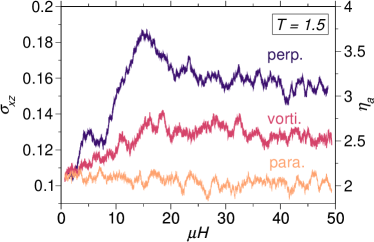
Figure 2: Shear stress as a function of the strength of an magnetic field with three different directions: (i) the direction parallel to $\mathbf{n}^{(0)}$, (ii) the vorticity direction, which is parallel to the $y$-axis, and (iii) the direction perpendicular to $\mathbf{n}^{(0)}$ in the $xz$-plane. The left vertical axis of the graph shows the shear stress, while the right vertical axis indicates the apparent viscosity, $\eta_{a}=\sigma_{xz}/\dot{\Gamma}$ with $\dot{\Gamma}=5\times 10^{-2}$ . For all the cases, temperature is set to $T=1.5$ .

The aforementioned non-monotonic behavior is persistent, as depicted in the upper panel of Fig. 3, at the lower temperatures $T=1.0$ and $T=0.75$, where the corresponding equilibrium system at $H=0$ is deep in the nematic state brown1998effects . Moreover, we find the same non-monotonic behavior also for slower and faster rates of changing $H$, as shown in Fig. 10 of Appendix B.

To shed light on the origin of this non-monotonic behavior, we now investigate the structure formation of the magnetic and non-magnetic particles at different values of the magnetic field and $T=1.5$ . The corresponding snapshots are shown in the lower panel of Fig. 3. They reveal a significant dependence of the orientational and translational structure on the external field. To quantify these magnetic field induced effects, we study, first, the structure of the system at $H=0$, which represents our reference system. Then we show that by increasing the magnetic field for zero, the deviation of the orientations of the MNPs from the shear-induced direction leads to an increase of the shear stress. By further increase of $H$, the aforementioned deviation increases and eventually causes demixing of the MNPs and LCs. Finally, we show that this demixing is correlated with the decrease of the stress at large $H$ values.

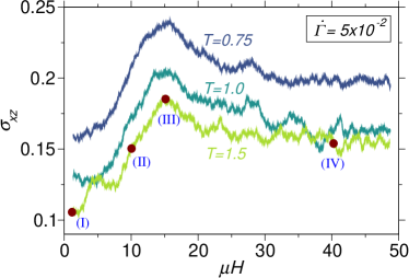
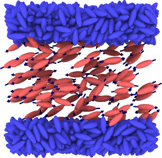
(I)         (II)

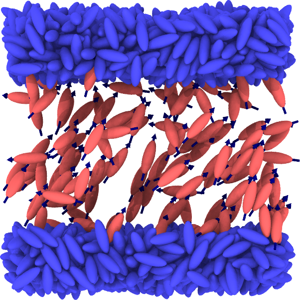
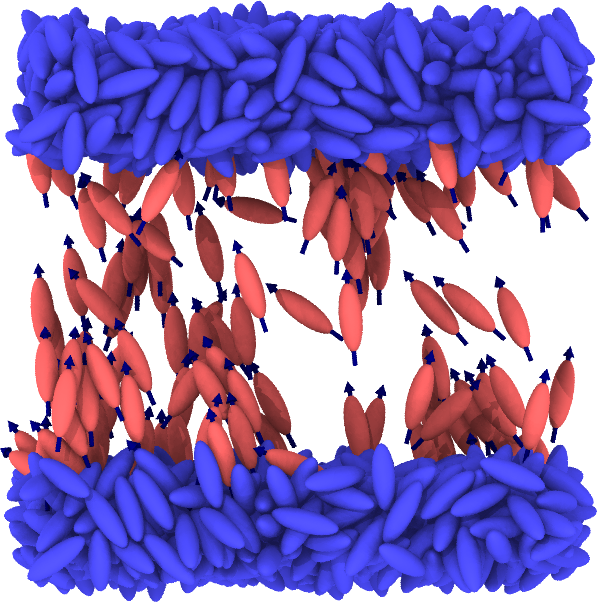
(III)     (IV) 

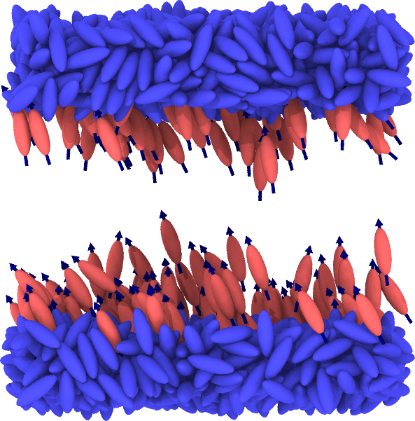
Figure 3: Upper panel: Shear stress as a function of the magnetic field strength at three different temperatures. Lower panel: Representative configurations associated with the four values of the field, which are indicated by bullets and the Roman numbers on the $T=1.5$ curve in the upper panel. For all simulations, $\dot{\Gamma}$ is kept fixed at $5\times 10^{-2}$ .

Upon shearing the system in absence of the magnetic field, we observe an increase in the order parameter $S_{\mathrm{LC(MNP)}}$ of particles, a phenomenon known as shear-induced ordering (see Ref. hess2004regular and references therein). In Fig. 4, the evolution of the nematic order parameter of the system as a function applied the strain, $\Gamma$ (or, equivalently, the time interval the system is sheared), is depicted for temperature $T=1.5$ and shear rate $\dot{\Gamma}=5\times 10^{-2}$. The results show that the system evolves from a state close to isotropic-nematic transition ($S\simeq 0.45$) to a nematic state ($S=0.65$). We recall that at $H=0$, the LCs and the MNPs are essentially indistinguishable, and therefore we report only one $S$ for the whole system.

Applying shear not only increase the nematic order parameter, but also changes the orientation of the nematic director. In Fig. 4, the angle between the nematic director and the shear direction (i.e. $x$-direction) is shown: the angle $\theta$ evolves from zero to its steady state value as the strain is increased. This steady state $\theta$ value, which is also known as the Leslie angle, is $\theta\simeq$$$ in our system for the previously specified parameters. The obtained value, although system specific, is close to the reported value by a previous GB study wu2007non .

Upon increasing the magnetic field strength from zero at the finite shear ($\dot{\Gamma}=5\times 10^{-2}$), the MNPs tend to align with $\hat{\mathbf{H}}$, inducing a competition with the shear-induced ordering along $\mathbf{n}^{(0)}$. As an illustration, we plot in Fig. 5 the nematic order parameters of each component, as well as the angles between the director of each component, $\hat{\mathbf{n}}_{\alpha}$, and the shear direction ($x$-direction). The nematic order parameter of the MNPs, $S_{\mathrm{MNP}}$, decreases for small values of $H$ . This is since the MNPs now tend to align with $\hat{\mathbf{H}}$, which is perpendicular to the nematic director in absence of the field, i.e. $\mathbf{n}^{(0)}$, see Fig. 5a. Interestingly, in the same range of $H$-values, the orientation of the nematic director is still same as for $H=0$, as seen from the behavior of $\theta_{\mathrm{MNP}}$ in Fig. 5b. Indeed, the behavior of the angle between the MNPs director and the shear direction is reminiscent of a Fréederickz transition freedericksz1927theoretisches ; freedericksz1933forces : Up to a threshold value of the external field , in this case $H_{\mathrm{th}}\simeq 5$, the director of magnetic particles is not deviating from $\mathbf{n}^{(0)}$. Upon further increase of the magnetic field, it suddenly starts deviating from $\mathbf{n}^{(0)}$, until it is fully aligned with the field direction, $\hat{\mathbf{H}}$. In this regime, increasing the magnetic field leads to an increase of $S_{\mathrm{MNP}}$ along the new director, as can be seen from Fig. 5a. We note that, unlike the conventional Fréederickz transition which is an equilibrium phenomenon, here the system is out of equilibrium. Also, in a conventional Fréederickz transition, the unperturbed direction is induced by the confinement, whereas here the unperturbed direction is the shear-induced direction.

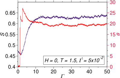
Figure 4: Plots of the nematic order parameter, $S$, and the angle between the nematic order director and $x$-axis, $\theta$, as functions of the strain, $\Gamma$ (in absence of the magnetic field). Shear leads to an increase in the nematic order parameter and it also changes the orientation of the director. In absence of shear, i.e. at $\Gamma=0$, the director is aligned parallel to the walls and upon shearing it starts deviation from that. In steady state, we find $\theta\simeq$$$, which is close to the value reported in an earlier study wu2007non .

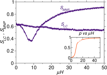
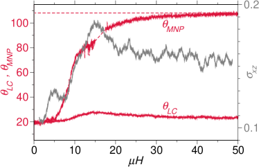
Figure 5: (a) Nematic order parameter for LCs and MNPs as a function of $\mu H$. The results show that, unlike $S_{\mathrm{MNP}}$, $S_{\mathrm{LC}}$ is not affected dramatically by the external field. The inset shows that $p=\mu^{-1}P$ has a weak dependence on $\mu H$ before $\mu H\simeq 5$, in contrast to its strong dependence for larger $\mu H$ values. (b) The left vertical axis of the graph shows the angles between the nematic directors, i.e. $\hat{\mathbf{n}}_{\mathrm{LC}}$ and $\hat{\mathbf{n}}_{\mathrm{MNP}}$), with the shear direction ($x$-direction). The value of the these angles coincide at $H=0$ where the LCs and MNPs are essentially indistinguishable. The right vertical axis of the graph shows the stress as a function of the external magnetic field strength. Similar to Fréderickz transition, up to a threshold value of the magnetic field (here $\mu H_{\mathrm{th}}\simeq 5$) the nematic director remains undistorted, and beyond that it start deviating from the $H=0$ direction, and eventually fully aligns with the direction of the magnetic field.

The field-dependence of the ordering of magnetic particles is also reflected by the polarization, $p=\mu^{-1}P$, which increases from zero by applying the magnetic field. As shown in Fig. 5a, a significant increase of $p$ occurs as the magnetic field exceeds $\mu H_{\mathrm{th}}$, although a slight increase is observed before this threshold.

As is visible from Fig. 5, not only the orientational order of the MNPs, but also that of the LCs is affected by the magnetic field, although the LCs themselves are not susceptible to the magnetic field. This is an indirect effect: The magnetic field re-orients the MNPs, which in turn, affects the orientation of the neighboring LCs due to the anisotropic steric interactions between the MNPs and LCs. However, considering that the MNPs form only a small fraction, the effect of the field on the LCs is small at the present condition, see Fig. 5.

In view of the competing effects of magnetic field and shear, we are now in a position to interpret the marked nonmonotonic behavior of the shear stress, $\sigma_{xz}$. Indeed, as seen from Fig. 5b, there is a clear correlation between the increase of $\sigma_{xz}$ and the misalignment of the MNPs at small to moderate values of $H$. This can be qualitatively understood by considering that $\sigma$ is proportional to $\tau$, where $\tau$ is the relaxation time of the system. We argue that $\tau$ is increasing by applying $H$, as applying magnetic field reduces orientational freedom of the MNPs, and hence making the relaxation process less likely. Here, by the relaxation process, we refer to the atomistic mechanism behind the stress relaxation, i.e. going from a configuration with high stress to another configuration with a lower stress Stillinger1995 ; Stillinger1982 ; Doliwa2003 ; Falk1998 ; Goldhirsch2002 ; Rabani1997 ; Lindemann1910 ; Ahn2013 ; siboni2015aging . It has been argued adam1965temperature ; richert1998dynamics ; mauro2009viscosity that, the probability of such transition is proportional to the configurational entropy of the system adam1965temperature ; richert1998dynamics ; mauro2009viscosity ; roughly speaking, it is more likely for a system to make a transition, if more states are available. In the studied system here, by confining the orientation of a fraction of particles in a particular direction via magnetic field, the configurational entropy is reduced, which leads to an increase in $\tau$ and $\sigma$.

So far, we have focused on the correlation between the field-induced orientational ordering of the magnetic particles and the shear stress. Upon further increase of the magnetic field to the point, where the misalignment between MNPs and LCs is close to its maximum, the shear stress shows a decrease. Interestingly, this decrease occurs simultaneously with a significant qualitative change in the spatial distribution of the MNPs. This qualitative change is illustrated by the four representative configurations at different values of $\mu H$, see Fig. 3: Starting from a relatively homogeneous distribution of MNPs at small $H$, further increase of $H$ leads to a demixing between MNPs and LCs. We quantify these structural transformations by measuring the averaged number density profile of MNPs as a function of the external field. The results are plotted in Fig. 6: At large field strengths (state points III and IV) one observes a pronounced double-peak structure of the MNPs density profile, reflecting the assembly of the MNPs at the walls. This is in a qualitative contrast with the uniform spatial distribution of the MNPs (and thus, also the LCs) at small $\mu H$ values.

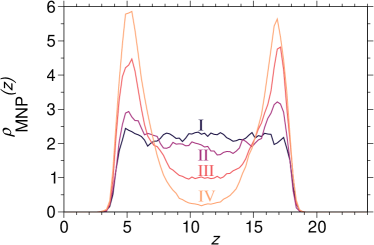
Figure 6: The density profiles of the MNPs at different magnetic field values. The roman numbers refer to the same numbers in Fig. 3. For small fields, a relatively uniform spatial distribution is obtained, in contrast to strong fields where a double-peaked profile emerges.

To better relate the field-induced changes of the spatial distribution and the stress behavior, we introduce an entropy-like measure which quantifies the degree of inhomogeneity of the density distribution of MNPs. Specifically, we consider the quantity

$$I[\tilde{\rho}]:=\int{\tilde{\rho}(z)\ln(\tilde{\rho}(z))dz}~{},$$ (4)

where $\tilde{\rho}(z)$ is the MNP density, $\rho_{\mathrm{MNP}}$, with normalization $\int_{0}^{L_{c}}\tilde{\rho}(z)dz=1$ .

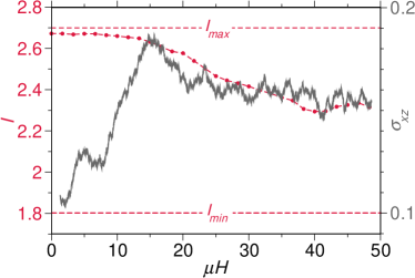
Figure 7: The entropy-like quantity of Eq. 4 as a measure of homogeneous distribution of the MNPs for different values of the external magnetic field strength. The data clearly shows that there is a transition from homogeneous spatial distribution of the MNPs to an inhomogeneous one.

The obtained $I$ as a function of the magnetic field is shown in Fig. 7. For comparison, we have also indicated the values of $I$ for two extreme cases: $I_{\mathrm{max}}$ which corresponds to an absolutely uniform distribution of MNPs, and $I_{\mathrm{min}}$, which refers to the case where all MNPs are concentrated close to walls in a region of width $\sigma_{l}=3$, the length corresponding to the large axis of the particles.

For small values of $H$, $I$ remains essentially equal to its value at $H=0$, which is close to $I_{\mathrm{max}}$ (reflecting a nearly homogeneous distribution). Only when $H$ becomes larger than the threshold value $\mu H\simeq 15$, $I$ starts to decrease, indicating the onset of demixing. Moreover, the overlay of the $H$ dependence of $I$ and $\sigma_{xy}$ in Fig. 7 shows that for larger field strengths, the stress decreases along with the $I$ decrease. These results confirm the correlation between onset of inhomogeneity and reduction of stress.

Having established the correlation between the demixing and the decrease of the shear stress, there remains the question for the underlying physical mechanism. Our interpretation is as follows: The “misalignment” of the MNPs at small fields leads to restrictions of the flow-induced motion of the non-magnetic ones, and hence, to an increase of the stress. However, this is true only if the MNPs are dispersed between the LCs. As soon as the system demixes [see Figs. (6)-(7)], that is, at large values of $\mu H$, the MNPs are concentrated close to the walls. This provides a channel for the LCs in which they can flow without (orientational and positional) disturbances from the MNPs.

Clearly, a key ingredient in this line of argumentation is the field-induced orientational mismatch between the MNPs and LCs. Our numerical results indicate that this mismatch alone leads to a demixing-like transition: We emphasize that the interactions between all the particles are identical, so the demixing cannot be attributed to different shapes or interactions between the two species, such as the demixing transitions reported in Refs. purdy2005nematic ; varga2005nematic ; bates1999nematic ; ferreiro2016spinodal ; helden2003direct ; roth2003entropic ; brader2002colloidal ; Tasinkevych2006 ; whitmer2013 ; adams1998entropically ; mizoshita2003fast . We further note that the demixing also occurs in bulk simulations (where the shear is induced via Lees-Edward boundary condition lees1972computer ), which emphasizes that the demixing is not due to the existence of the walls.

We propose that the observed demixing between particles of different orientations can be understood as a competition between mixing entropy and packing entropy. Qualitatively speaking, on the one hand, it is preferable for the system if particles with the same orientations stay close to each other as this leads to larger (orientational) free volumes for each particle. On the other hand, more (positional) configurations are available to the system if the particles are uniformly distributed in the system irrespective of their orientations. In other words, an increase in packing entropy is obtained when particles of similar orientations are neighbors, and whereas higher mixing entropy is reached when particles are uniformly distributed over the whole system. In our system, at small fields, where the misalignment is not yet pronounced, the mixing entropy dominates and the MNPs are uniformly distributed between the LCs. In contrast, at large fields, where the misalignments are large, the system gains entropy by bringing particles of similar orientation close to each other (and hence demixing).

In Appendix D, by using a simplified Onsager analysis onsager1949effects for binary mixtures lekkerkerker1984isotropic , we argue that particle misalignments are indeed sufficient to to cause demixing. We show that the free energy difference between the demixed state and the fully mixed state of long, hard ellipsoids can be written as

$$\Delta\mathcal{F}=(1-x)\ln(1-x)+x\ln(x)+2cb_{\perp}x(1-x)|\sin(\Theta)|~{},$$ (5)

where $c$ is the number density, $b_{\perp}$ is the excluded volume of two ellipsoids in perpendicular configuration onsager1949effects , and $\Theta$ is the angle measuring the degree of misalignment. In the present case, $\Theta$ is essentially determined by the magnetic field. We find from Eq. 5 that, there is a critical density below which mixing is favored, whereas above it, depending on the misalignment between the directions ($\Theta$) and composition ($x$), demixing is favored. Although the aforementioned Onsager analysis relies on equilibrium arguments, it does suggest that demixing in the present nonequilibrium system is possible.

Experimentally, a similar demixing has been realized in a system of nano-rods van2010onsager , where a certain degree of polydispersity is required to induce particle misalignments. In contrast to that, in our study, the demixing occurs between monodisperse particles. This isolates the role of orientational misalignments. Moreover, we want to emphasize that, in contrast to Ref. van2010onsager , being out-of-equilibrium is essential for the observed demixing in our system as one of the favored orientations is the shear-induced orientation.

IV Conclusion and Outlook

In this study, we performed a NEMD study of a mixture of anisotropic magnetic and non-magnetic particles confined between two rough solid walls, focusing on the shear stress in the presence of an external magnetic field. In our model, the interactions between both types of particles are the same; The only difference between the magnetic and non-magnetic particles is that the field acts solely on the direction of the magnetic particles. Our simulation results indicate that the obtained shear stress depends on the strength and direction of the external field. More specifically, for a field direction within shear-plane and perpendicular to the shear-induced nematic director, we observe a non-monotonic dependence of shear stress and thus, the viscosity, on the applied field strength. Such a non-monotonic behavior is in sharp contrast with the observed monotonic behavior in ferrofluids odenbach2004recent . By analyzing the nematic director of the LCs and MNPs, we have found that the increase in the shear stress is correlated to the misalignment of the MNP director relative to the shear-induced director of the majority of particles, i.e. the LC particles. The shear stress increases up to the point that the misalignment is sufficient to cause an entropic demixing between the MNPs and LCs. The occurrence of demixing is also (qualitatively) predicted by a simplified Onsager analysis. Unlike previously analyzed systems where the effective entropic interaction is due to size-polydispersity purdy2005nematic ; varga2005nematic ; bates1999nematic ; ferreiro2016spinodal or shape-polydispersity helden2003direct ; roth2003entropic ; brader2002colloidal ; Tasinkevych2006 ; whitmer2013 ; adams1998entropically ; mizoshita2003fast , in our system the underlying mechanism is due to (competing) orientations. This is an interesting case of an effective interaction where there is no difference in shape and inter-particle interaction between the particles constituting different groups. This extends the notion of the directional entropic forces, introduced in Refs. Damasceno2011 ; vanAnders2013entropically , to a system where the particles are much simpler in their shape.

Given the complex response observed in the present study, one would expect even more diverse behavior when dipole-dipole interaction between the MNPs are included. The rheology of MNP/LC mixture in external magnetic field over a range of dipole-dipole couplings will be subject of further studies. Indeed, as it is known for systems of pure anisotropic MNPs, the dipole-dipole interaction can lead to self-assembled structures which can be significantly different from the chain formation observed schmidle2012phase in systems of spherical MNPs. In particular, for MNPs with large enough aspect ratio the neighboring particles prefer formations with anti-parallel configurations mcgrother1998effect ; alvarez2012percolation . We speculate that such formation of a structured phase within the liquid phase has important consequences for the rheological properties of the mixture, similar to the effect of including crystalline microstructures in amorphous bulk metallic glasses hofmann2008designing ; hays2000microstructure ; guo2014shear . We also expect that the external field has an important effect on the rheology: As the external field disfavors the anti-parallel dipoles, the stability of the assembled structures of MNPs is reduced alvarez2012percolation , which can lead to dissolving these structures in the liquid phase.

In this study, we only focused on the case where the dipoles are aligned with the longest axis of the ellipsoid. The anisotropic shape of the MNPs also offers the possibility of aligning the magnetic dipole along different axes of the particles. For further studies, one can consider embedding the magnetic dipoles along the shortest axis, as done in recent experiments martinez2016dipolar , or include an offset from the center as done for spherical particles kantorovich2011ferrofluids ; klinkigt2013cluster ; morphew2016supracolloidal ; steinbach2016non ; yener2016self ; rutkowski2017simulation . Depending on different embeddings, by increasing the dipole-dipole interaction strength we speculate to find intriguing structures where an external magnetic field can play an important role in stabilizing or destabilizing them.

Appendix A Effects of walls

Strong confinement can lead to structural and dynamical properties which are significantly different from bulk properties gruhn1997microscopic ; mazza2010entropy . Nevertheless, if the confinement is not severe, one would expect the sample to behave similar to the bulk. In this appendix, we argue that although the system studied here has walls and is therefore confined, the wall effects are negligible at the current wall-to-wall separation. To this end, we first compare the nematic order (in absence of the magnetic field and shear) as a function of temperature for two systems: the system without walls (i.e. the system with the periodic boundary conditions in all directions), and the same system after creating walls by freezing the wall particles, as explained in the main text (see Section II). In Fig. 8, the nematic order of the system in presence of wall is shown over a range of temperatures. Also indicated is the value of $S$ at the main working temperature, i.e. $T=1.5$ , in presence of walls. It is seen that the change in $S$, as a result of introducing walls, is negligible. One should note that, as the system at $T=1.5$ is very close to its isotropic-to-nematic transition, one would expect a relatively high sensitivity of $S$ on the ambient changes, including introducing walls. Even under these conditions, introducing walls does not change $S$, which is an indication that the walls do not dominate the behavior of the system.

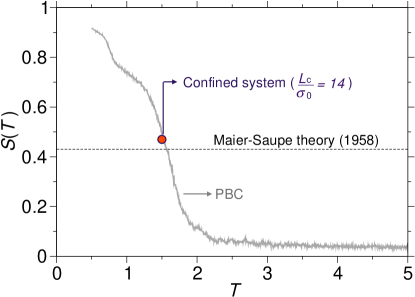
Figure 8: Nematic order parameter as a function of temperature. The gray line pertains to the system with the full periodic boundary conditions, and the orange dot presents the value of $S$ for the same system at $T=1.5$, after creation of the walls, as explained in Section II. The horizontal dashed line represent the approximate critical nematic order parameter maier1958einfache ; maier1959einfache ; maier1960einfache , $S_{c}\simeq 0.43$, above which the system is considered to be in the nematic phase. The main working temperature is chosen such that the system is very close to isotopic to nematic state transition ($S\simeq 0.45$).

As a second point, we check the effect of the walls in presence of shear flow by measuring the density and shear rate profiles across the channel (along $z$-direction) at different strength of the external field. The local density is obtained as described in Section II, and the local shear rate is obtained by $\dot{\gamma}(z):=\frac{d}{dz}v_{x}(z)$, where $v_{x}(z_{0})$ is the average $x$-component of velocities of all particles between planes $z=z_{0}-\delta z/2$ and $z=z_{0}+\delta z/2$, and $\delta z=0.25$ is the descritization resolution along the $z$-axis. The obtained velocity, shear rate, and density profiles are shown in Fig. 9, for $T=1.5$ and $\dot{\Gamma}=5\times 10^{-2}$ . The velocity profile shows that the flow is almost independent of the magnetic field strength. This is remarkable given that the composition profile and also the average orientations strongly depend on the magnetic field strength. The shear rate profile, plotted in the inset of Fig. 9, shows that there is no slip close to the walls, and that the wall effects on the dynamics (here the local shear rate) reach from the wall into the bulk of the system over a length of about $\simeq 3\sigma_{0}$. The same is valid for the local density of all particles.

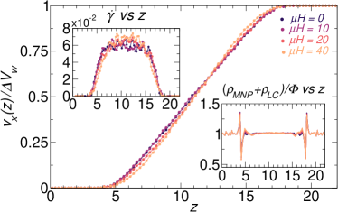
Figure 9: The velocity profile, $v_{x}(z)$ which is the average velocity along $x$-direction as a function of $z$ at $T=1.5$ and four different values of $\mu H$. The local shear-rate, $\dot{\gamma}(z)=\frac{d}{dz}v_{x}(z)$, and the local particle density (including both MNP and LC particles) are shown in the insets. There is no indication of slip as there is no discontinuity of the shear rate across the boundary. The condition at the boundary can be approximated with no slip boundary condition with where the boundary effects are present up to $3\sigma_{0}$.

Appendix B Dependence of the shear stress on the field protocol

In this study, as mentioned in Section II, the magnetic field is increased gradually from zero to $H_{\mathrm{max}}$ over the time interval $t_{\mathrm{max}}$, i.e. with the rate of $\frac{dH}{dt}=\frac{H_{\mathrm{max}}}{t_{\mathrm{max}}}$. Here we check whether the non-monotonic behavior, which is the subject of this study, is affected by changing the values of $\frac{dH}{dt}$. The magnetic field dependence of the shear stress is shown in Fig. 10, for a range of $\frac{dH}{dt}$ values. The rates are chosen both larger and smaller than the rate used primarily in this work, which corresponds to $\mu\frac{dH}{dt}=0.033$ . Similar to the temperature dependence of shear stress (see Fig. 3), the results in Fig. 10 show that, although the $\sigma_{xz}$-$H$ curve changes quantitatively for different $\frac{dH}{dt}$ values, its non-monotonic behavior is not affected at qualitative level for the examined $\frac{dH}{dt}$ values.

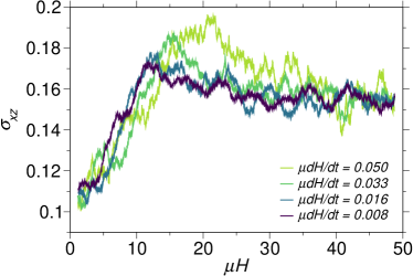
Figure 10: Shear stress as a function of the magnetic field strength for different values of $\frac{dH}{dt}$ at $T=1.5$. The results show that, in spite of quantitative differences, the qualitative dependence of the shear stress on $H$ does not depend on the $dH/dt$ value (within the considered range of values).

Appendix C Stress auto-correlation function

Applying shear as an external perturbation leads to the response of the system in the form of an increase of the shear stress. In the liquid phase, there is a finite characteristic time, usually referred to as the relaxation time, which the system needs to adapt to the induced stress (i.e. to reduce it to zero). This relaxation time is used to distinguish between high and low shear rates: if the inverse shear rate is much larger than the relaxation time, the applied shear rate is considered to be slow compared to the relaxation of the system and one would expect a linear response of the system. Here, we calculate the relaxation time associated with stress, $\tau_{\sigma}$. In order to calculate such a relaxation time, we analyze the stress auto-correlation, $C_{\sigma}(t):=\langle\sigma_{xz}(t)\sigma_{xz}(0)\rangle/\langle\sigma_{xz}^{2}(0)\rangle$, which is calculated in absence of shear. Here, $\langle.\rangle$ refers to an ensemble average. As shown in Fig. 11, the stress auto-correlation decays to zero and one can assign an approximate time to this decay. For $T=1.5$, the obtained relaxation time is $\tau_{\sigma}\simeq 1$ .

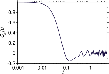
Figure 11: The shear stress auto-correlation function, measured at $T=1.5$ and in absence of shear, which shows that after time $t\simeq 1$ the stress auto-correlation decays to zero.

Appendix D Simplified Onsager analysis

In this Appendix, by using a simplified version of the Onsager analysis presented in Refs. onsager1949effects ; lekkerkerker1984isotropic , we show that for a system composed of hard ellipsoids of identical shapes, an orientational misalignment between the particles is sufficient to cause a demixing. More specifically, we consider a system composed of two particle species $A$ and $B$, and the corresponding one-particle orientation distribution functions, $f_{A}$ and $f_{B}$. We show that under certain constrains, the free-energy of the system is minimized if the two particle species are spatially demixed.

For simplicity and without loss of generality, we assume that $f_{A}$ and $f_{B}$ are given by the Dirac delta distribution located at $\hat{\mathbf{n}}_{A}$ and $\hat{\mathbf{n}}_{B}$, i.e. the average nematic directions. We also assume a canonical ensemble with total fixed particle number $N=N_{A}+N_{B}$, volume $V$, and temperature $T$, where $N_{A}$ and $N_{B}$ are the numbers of particles in species $A$ and $B$. We are interested in the free energy of the system when (i) both particle species are homogeneously distributed ($F_{\mathrm{hom.}}$), and (ii) particles of different species are separated from each other completely ($F_{\mathrm{inh.}}$).

Following Ref. lekkerkerker1984isotropic , the reduced free energy per particle for a spatially homogeneous distribution, i.e. $\mathcal{F}_{\mathrm{hom.}}=F_{\mathrm{hom.}}/(Nk_{\mathrm{B}}T)$, reads

$$\mathcal{F}_{\mathrm{hom.}} =1+\ln(c)+(1-x)\ln(1-x)+x\ln(x)$$

$$\quad+(1-x)\sigma[f_{A}]+{x\sigma[f_{B}]}$$

$$\quad+cb_{\parallel}(1-x)^{2}\rho[f_{A},f_{A}]+cb_{\parallel}{x^{2}\rho[f_{B},f_{B}]}$$

$$\quad+2cb_{\perp}x(1-x)\rho[f_{A},f_{B}]~{},$$ (6)

where $x$ is the fraction of $B$ particles, $c=N/V$ is the overall number density, $b_{\parallel}=\pi/L^{2}D$, and $b_{\perp}\simeq L^{2}D$, with $b_{\parallel}$ and $b_{\perp}$ being the excluded volumes of two long ellipsoids of length $L$ and diameter $D$ in parallel and perpendicular configurations onsager1949effects . In the above equation, the functional $\sigma[f]$ measures the entropy associated with the distribution $f$ itself, and $\rho[f,f^{\prime}]$ measures the entropy associated with the volume available to neighboring particles with two distributions $f$ and $f^{\prime}$ (the exact expressions can be found in Onsager’s work onsager1949effects ). Assuming $L\gg D$, that is, a needle-like shape, $\mathcal{F}_{\mathrm{hom.}}$ can be approximated by

$$\mathcal{F}_{\mathrm{hom.}} =1+\ln(c)+(1-x)\ln(1-x)+x\ln(x)$$

$$\quad+2cb_{\perp}x(1-x)|\sin(\Theta)|~{},$$ (7)

where $\Theta$ is the angle between $\hat{\mathbf{n}}_{A}$ and $\hat{\mathbf{n}}_{B}$. Similarly, we obtain a reduced free energy for the case where the species $A$ and $B$ are spatially separated. In this case, the free energy per particle for each of the species is obtained by setting $x$ to zero, as each phase is purely composed of one species. This leads to

$$\mathcal{F}_{\mathrm{inh.}} =1+\ln(c)~{},$$ (8)

where the free-energy associated with the boundary between the two groups is neglected. The difference between the free energies in the demixed state and that in the mixed state, $\Delta\mathcal{F}=\mathcal{F}_{\mathrm{inh.}}-\mathcal{F}_{\mathrm{hom.}}$, is given by

$$\Delta\mathcal{F}=(1-x)\ln(1-x)+x\ln(x)+2cb_{\perp}x(1-x)|\sin(\Theta)|~{}.$$ (9)

The first two terms on the right side of Eq. 9 are always negative and thus favor a mixed system, while the third term is always positive and thus favors demixing. The magnitude of the third term increases by increasing $\Theta$, which might eventually lead to a sign change for $\Delta\mathcal{F}$. It is straightforward to show that, depending on the values of $\Theta$ and $x$, $\Delta\mathcal{F}$ can become positive. In particular, one can show that there is a critical density $c_{\mathrm{cr}}$ (with $c_{\mathrm{cr}}b_{\perp}=2\ln(2)$), below which always mixing is favored.

References

- (1) F. Brochard and P. de Gennes, J. Physique 31, 691 (1970).
- (2) J. Rault, P. Cladis, and J. Burger, Phys. Lett. A 32, 199 (1970).
- (3) A. Mertelj, D. Lisjak, M. Drofenik, and M. Čopič, Nature 504, 237 (2013).
- (4) A. Mertelj, N. Osterman, D. Lisjak, and M. Čopič, Soft Matter 10, 9065 (2014).
- (5) Q. Liu, P. J. Ackerman, T. C. Lubensky, and I. I. Smalyukh, Proc. Natl. Acad. Sci. U. S. A. 113, 10479 (2016).
- (6) N. Podoliak, O. Buchnev, D. V. Bavykin, A. N. Kulak, M. Kaczmarek, and T. J. Sluckin, J. Colloid Interface Sci. 386, 158 (2012).
- (7) P. Kopčanskỳ, N. Tomašovičová, M. Koneracká, V. Závišová, M. Timko, A. Džarová, A. Šprincová, N. Éber, K. Fodor-Csorba, T. Tóth-Katona, et al., Phys. Rev. E 78, 011702 (2008).
- (8) S. D. Peroukidis, K. Lichtner, and S. H. Klapp, Soft Matter 11, 5999 (2015).
- (9) S. D. Peroukidis and S. H. Klapp, Phys. Rev. E 92, 010501(R) (2015).
- (10) S.-H. Chen and N. M. Amer, Phys. Rev. Lett. 51, 2298 (1983).
- (11) A. V. Kyrylyuk, M. C. Hermant, T. Schilling, B. Klumperman, C. E. Koning, and P. Van der Schoot, Nature nanotechnology 6, 364 (2011).
- (12) O. Buluy, S. Nepijko, V. Reshetnyak, E. Ouskova, V. Zadorozhnii, A. Leonhardt, M. Ritschel, G. Schönhense, and Y. Reznikov, Soft Matter 7, 644 (2011).
- (13) F. Martinez-Pedrero, A. Cebers, and P. Tierno, Phys. Rev. Appl. 6, 034002 (2016).
- (14) S. Kredentser, M. Kulyk, V. Kalita, K. Slyusarenko, V. Y. Reshetnyak, and Y. A. Reznikov, Soft Matter 13, 4080 (2017).
- (15) N. Sebastián, N. Osterman, D. Lisjak, M. Čopič, and A. Mertelj, Soft Matter 14, 7180 (2018).
- (16) T. Potisk, A. Mertelj, N. Sebastián, N. Osterman, D. Lisjak, H. R. Brand, H. Pleiner, and D. Svenšek, Phys. Rev. E 97, 012701 (2018).
- (17) G. Zarubin, M. Bier, and S. Dietrich, Soft Matter 14, 9806 (2018).
- (18) G. Zarubin, M. Bier, and S. Dietrich, J. Chem. Phys. 149, 054505 (2018).
- (19) R. Blaak, S. Auer, D. Frenkel, and H. Löwen, J. Phys.: Condens. Matter 16, S3873 (2004).
- (20) M. Ripoll, P. Holmqvist, R. Winkler, G. Gompper, J. Dhont, and M. Lettinga, Phys. Rev. Lett. 101, 168302 (2008).
- (21) A. V. Mokshin and J.-L. Barrat, Phys. Rev. E 77, 021505 (2008).
- (22) S. Mandal, M. Gross, D. Raabe, and F. Varnik, Phys. Rev. Lett. 108, 098301 (2012).
- (23) G. P. Shrivastav, P. Chaudhuri, and J. Horbach, Journal of Rheology 60, 835 (2016).
- (24) N. Kikuchi and J. Horbach, EPL 77, 26001 (2007).
- (25) E. Zaccarelli, S. M. Liddle, and W. C. Poon, Soft Matter 11, 324 (2015).
- (26) D. Heckendorf, K. Mutch, S. Egelhaaf, and M. Laurati, Phys. Rev. Lett. 119, 048003 (2017).
- (27) C. Ferreiro-Córdova and H. Wensink, J. Chem. Phys. 145, 244904 (2016).
- (28) A. Verhoeff, H. Wensink, M. Vis, G. Jackson, and H. Lekkerkerker, J. Phys. Chem. B 113, 13476 (2009).
- (29) A. Speranza and P. Sollich, J. Chem. Phys. 117, 5421 (2002).
- (30) C. E. Alvarez and S. H. Klapp, Soft Matter 8, 7480 (2012).
- (31) H. Schmidle, C. K. Hall, O. D. Velev, and S. H. Klapp, Soft Matter 8, 1521 (2012).
- (32) A. Sreekumari and P. Ilg, Phys. Rev. E 88, 042315 (2013).
- (33) K. May, A. Eremin, R. Stannarius, S. D. Peroukidis, S. H. Klapp, and S. Klein, Langmuir 32, 5085 (2016).
- (34) S. D. Peroukidis and S. H. Klapp, Soft Matter 12, 6841 (2016).
- (35) G. P. Shrivastav and S. H. Klapp, Soft Matter 15, 973 (2019).
- (36) S. Odenbach, J. Phys.: Condens. Matter 16, R1135 (2004).
- (37) R. Rosensweig, R. Kaiser, and G. Miskolczy, J. Colloid Interface Sci. 29, 680 (1969).
- (38) W. Hall and S. Busenberg, J. Chem. Phys. 51, 137 (1969).
- (39) M. Shliomis, Zh. Eksp. Teor. Fiz 61, s1971d (1971).
- (40) R. Berardi, C. Fava, and C. Zannoni, Chem. Phys. Lett. 297, 8 (1998).
- (41) S. Plimpton, J. Comput. Phys. 117, 1 (1995).
- (42) L. Verlet, Phys. Rev. 159, 98 (1967).
- (43) W. C. Swope, H. C. Andersen, P. H. Berens, and K. R. Wilson, J. Chem. Phys. 76, 637 (1982).
- (44) J. T. Brown, M. P. Allen, E. M. del Río, and E. de Miguel, Phys. Rev. E 57, 6685 (1998).
- (45) N. H. Siboni, D. Raabe, and F. Varnik, Phys. Rev. E 87, 030101 (2013).
- (46) F. Varnik, L. Bocquet, J.-L. Barrat, and L. Berthier, Phys. Rev. Lett. 90, 095702 (2003).
- (47) M. Hassani, P. Engels, and F. Varnik, EPL 121, 18005 (2018).
- (48) D. J. Evans and G. P. Morriss, Phys. Rev. Lett. 56, 2172 (1986).
- (49) P. A. Thompson and M. O. Robbins, Phys. Rev. Lett. 63, 766 (1989).
- (50) P. A. Thompson and M. O. Robbins, Phys. Rev. A 41, 6830 (1990).
- (51) T. Soddemann, B. Dünweg, and K. Kremer, Phys. Rev. E 68, 046702 (2003).
- (52) X. Zhou, D. Andrienko, L. Delle Site, and K. Kremer, EPL 70, 264 (2005).
- (53) F. Varnik, J. Chem. Phys. 125, 164514 (2006).
- (54) A. Niavarani and N. V. Priezjev, Phys. Rev. E 77, 041606 (2008).
- (55) D. S. Bolintineanu, J. B. Lechman, S. J. Plimpton, and G. S. Grest, Phys. Rev. E 86, 066703 (2012).
- (56) K. S. Cheung and S. Yip, J. Appl. Phys. 70, 5688 (1991).
- (57) B. Todd, D. J. Evans, and P. J. Daivis, Phys. Rev. E 52, 1627 (1995).
- (58) F. Schwabl and W. D. Brewer, Statistical Mechanics, 2nd ed. (Springer Science & Business Media, Berlin Heidelberg, 2006).
- (59) F. M. Leslie, Arch. Ration. Mech. Anal. 28, 265 (1968).
- (60) W. Maier and A. Saupe, Z. Naturforsch. A 13, 564 (1958).
- (61) W. Maier and A. Saupe, Z. Naturforsch. A 14, 882 (1959).
- (62) W. Maier and A. Saupe, Z. Naturforsch. A 15, 287 (1960).
- (63) S. Hess and M. Kröger, J. Phys.: Condens. Matter 16, S3835 (2004).
- (64) C. Wu, T. Qian, and P. Zhang, Liq. Cryst. 34, 1175 (2007).
- (65) V. Fréedericksz and A. Repiewa, Zeitschrift für Physik 42, 532 (1927).
- (66) V. Fréedericksz and V. Zolina, Trans. Faraday Soc. 29, 919 (1933).
- (67) F. H. Stillinger, Science 267, 1935 (1995).
- (68) F. H. Stillinger and T. A. Weber, Phys. Rev. A 25, 978 (1982).
- (69) B. Doliwa and A. Heuer, Phys. Rev. E 67, 030501 (2003).
- (70) M. L. Falk and J. S. Langer, Phys. Rev. E 57, 7192 (1998).
- (71) I. Goldhirsch and C. Goldenberg, Eur. Phys. J. E 9, 245 (2002).
- (72) E. Rabani, J. D. Gezelter, and B. J. Berne, J. Chem. Phys. 107, 6867 (1997).
- (73) F. A. Lindemann, Phys. Z. 11, 609 (1910).
- (74) J. W. Ahn, B. Falahee, C. Del Piccolo, M. Vogel, and D. Bingemann, J. Chem. Phys. 138, 12A527 (2013).
- (75) N. H. Siboni, D. Raabe, and F. Varnik, EPL 111, 48004 (2015).
- (76) G. Adam and J. H. Gibbs, J. Chem. Phys. 43, 139 (1965).
- (77) R. Richert and C. Angell, J. Chem. Phys. 108, 9016 (1998).
- (78) J. C. Mauro, Y. Yue, A. J. Ellison, P. K. Gupta, and D. C. Allan, Proc. Natl. Acad. Sci. U. S. A. 106, 19780 (2009).
- (79) K. R. Purdy, S. Varga, A. Galindo, G. Jackson, and S. Fraden, Phys. Rev. Lett. 94, 057801 (2005).
- (80) S. Varga, K. Purdy, A. Galindo, S. Fraden, and G. Jackson, Phys. Rev. E 72, 051704 (2005).
- (81) M. A. Bates and D. Frenkel, J. Chem. Phys. 110, 6553 (1999).
- (82) L. Helden, R. Roth, G. H. Koenderink, P. Leiderer, and C. Bechinger, Phys. Rev. Lett. 90, 048301 (2003).
- (83) R. Roth, J. Brader, and M. Schmidt, EPL 63, 549 (2003).
- (84) J. M. Brader, A. Esztermann, and M. Schmidt, Phys. Rev. E 66, 031401 (2002).
- (85) M. Tasinkevych and D. Andrienko, Eur. Phys. J. E 21, 277 (2006).
- (86) J. K. Whitmer, A. A. Joshi, T. F. Roberts, and J. J. de Pablo, J. Chem. Phys. 138, 194903 (2013).
- (87) M. Adams, Z. Dogic, S. L. Keller, and S. Fraden, Nature 393, 349 (1998).
- (88) N. Mizoshita, K. Hanabusa, and T. Kato, Adv. Funct. Mater. 13, 313 (2003).
- (89) A. Lees and S. Edwards, J. Phys. C: Solid State Phys. 5, 1921 (1972).
- (90) L. Onsager, Ann. N. Y. Acad. Sci. 51, 627 (1949).
- (91) H. N. W. Lekkerkerker, P. Coulon, R. Van Der Haegen, and R. Deblieck, J. Chem. Phys. 80, 3427 (1984).
- (92) E. Van den Pol, A. Lupascu, M. Diaconeasa, A. Petukhov, D. Byelov, and G. Vroege, J. Phys. Chem. Lett. 1, 2174 (2010).
- (93) P. F. Damasceno, M. Engel, and S. C. Glotzer, ACS Nano 6, 609 (2011).
- (94) G. van Anders, N. K. Ahmed, R. Smith, M. Engel, and S. C. Glotzer, ACS Nano 8, 931 (2013).
- (95) S. C. McGrother, A. Gil-Villegas, and G. Jackson, Mol. Phys. 95, 657 (1998).
- (96) D. C. Hofmann, J.-Y. Suh, A. Wiest, G. Duan, M.-L. Lind, M. D. Demetriou, and W. L. Johnson, Nature 451, 1085 (2008).
- (97) C. Hays, C. Kim, and W. L. Johnson, Phys. Rev. Lett. 84, 2901 (2000).
- (98) W. Guo, E. A. Jägle, P.-P. Choi, J. Yao, A. Kostka, J. M. Schneider, and D. Raabe, Phys. Rev. Lett. 113, 035501 (2014).
- (99) S. Kantorovich, R. Weeber, J. J. Cerda, and C. Holm, Soft Matter 7, 5217 (2011).
- (100) M. Klinkigt, R. Weeber, S. Kantorovich, and C. Holm, Soft Matter 9, 3535 (2013).
- (101) D. Morphew and D. Chakrabarti, Soft Matter 12, 9633 (2016).
- (102) G. Steinbach, S. Gemming, and A. Erbe, Eur. Phys. J. E 39, 69 (2016).
- (103) A. B. Yener and S. H. Klapp, Soft Matter 12, 2066 (2016).
- (104) D. M. Rutkowski, O. D. Velev, S. H. Klapp, and C. K. Hall, Soft Matter 13, 3134 (2017).
- (105) T. Gruhn and M. Schoen, Phys. Rev. E 55, 2861 (1997).
- (106) M. G. Mazza, M. Greschek, R. Valiullin, J. Kärger, and M. Schoen, Phys. Rev. Lett. 105, 227802 (2010).