High dimensional parameter tuning for event generators

Abstract

Monte Carlo Event Generators are important tools for the understanding of physics at particle colliders like the LHC. In order to best predict a wide variety of observables, the optimization of parameters in the Event Generators based on precision data is crucial. However, the simultaneous optimization of many parameters is computationally challenging. We present an algorithm that allows to tune Monte Carlo Event Generators for high dimensional parameter spaces. To achieve this we first split the parameter space algorithmically in subspaces and perform a Professor tuning on the subspaces with bin wise weights to enhance the influence of relevant observables. We test the algorithm in ideal conditions and in real life examples including tuning of the event generators Herwig 7 and Pythia 8 for LEP observables. Further, we tune parts of the Herwig 7 event generator with the Lund string model.

I Introduction and Motivation

The amount of data taken at the LHC allows measuring observables that can be calculated perturbatively to high precision. This is beneficial for the comparison as well as the improvement of phenomenologically motivated non-perturbative models and also the searches for new physics. With the increasing precision made available in recent years through perturbative higher order calculations, theoretical uncertainties have reduced dramatically. In the comparison of these theory predictions and experimental data, Monte Carlo event generators (MCEG) (Buckley et al., 2011) like Herwig 7 (Bähr et al., 2008; Bellm et al., 2016a; Platzer and Gieseke, 2012; Bellm et al., 2017), Sherpa (Gleisberg et al., 2004) or Pythia 8 (Sjöstrand et al., 2006, 2015) play an important role. If possible a matched calculation that includes the perturbative corrections and the effects described by the MCEG can give an improved picture of the event structure measured by the experiment.

Here event generators typically include additional phenomenological models to include effects that are not part of specialised fixed order and resummed calculations. Uncertainties of these additional modelled, but factorised, parts of the simulation can be estimated from lower order simulations. The MCEG contain various, usually factorized (e.g. by energy scales) components. In the development, these parts can be improved individually. The afore mentioned matching to perturbative calculations is an example of recombining parts usually separated in the event generation, namely the parton shower and hard matrix element calculation. While it is possible to make such modifications and improvements, it is also necessary to keep other parts of the simulation in mind. Even though the generation is factorized, various parts of the simulation will have an impact on other ingredients of the generator. Any modification can, in general, have an impact on the full events. Calculated, or at least theoretically motived improvements will lead to a reduction of freedom that eventually also restricts the parameter ranges of the phenomenological models that could be used to compensate the variations of the perturbative side (Reichelt et al., 2017; Gieseke et al., 2018; Höche and Prestel, 2017; Höche et al., 2017; Bellm, 2018; Duncan and Kirchgaeßer, 2019; Dulat et al., 2018; Bewick et al., 2019). The capability to describe data needs to be reviewed with the modifications made in order to use the event generator for future predictions or concept designs for new experiments.

The procedure of adjusting the parameters of the simulation to measured data is called tuning. Various contributions for the tuning of MCEGs have been made (Barate et al., 1998; Hamacher and Weierstall, 1995; Abreu et al., 1996; Skands, 2009; Buckley et al., 2010; Skands et al., 2014; Khachatryan et al., 2016; Ilten et al., 2017; Buckley and Schulz, 2018), and the importance of these studies can be deduced from the recognition received. More recently, new techniques have been presented that can improve the performance of tuning (Bellm et al., 2016b; Mrenna and Skands, 2016; Bothmann et al., 2016; Bothmann and Debbio, 2019; Andreassen and Nachman, 2019). To be able to perform the comparison of simulation and data, the data needs to be collected and it needs to be possible to analyse the simulations similar to the experimental setup. Here, the hepdata project (Maguire et al., 2017) and analysis programs like Rivet (Buckley et al., 2013) are of great importance to the high energy physics community. Once the data and the possibility to analyse is given, the ’art’ of tuning is to choose the ’right’ data, possibly enhance the importance of some data sets over others, and to modify the parameters of the simulation such to reduce the difference of data and simulation. A prominent tool to allow the experienced physicist to perform the tuning is the Professor (Buckley et al., 2010) package that allows performing most of the procedure automatically.

The complexity of the MCEG tuning depends on the dimension of the parameter space used as an input to the event generation. Further, the measured observables are in general functions of many of the parameters used in the simulation. In this contribution, we address the problems of high dimensional parameter determination. We propose a method to choose subsets of parameters to reduce the complexity. We further aim to automatize the tuning process, to be able to retune with minimal effort once improvement is made to the MCEG in use. We call this automation of the tuning process and the algorithm to perform it the Autotunes method. As possible real life scenarios we then tune the Herwig 7 and Pythia 8 models and also a hybrid form, namely the Herwig 7 showers with the Pythia 8’s Lund String model (Andersson et al., 1983; Sjöstrand, 1984).

We structure the paper as follows: In Section II we define the problem and questions that we want to solve and answer. We then describe Professor and its the capabilities and restrictions. In Section III we explicitly define the algorithm and point out how the methods used will act mathematically. In Section IV we show how the algorithm was tested. Results of tuning the event generators Herwig 7 and Pythia 8 are presented in Section V. We conclude in Section VI and specify the possible next steps.

II Current State

Monte Carlo event generators provide theoretical predictions based on different physics aspects. Some of these, like the generation of the hard process, are derived from ’first principles’ and include just a few parameters like the coupling strength. The implementation of parton showers involves a number of physics choices, like the ordering variable, which can affect the predictions. Due to the breakdown of the perturbative description of QCD at low energy scales, a transition to the non-perturbative regime has to be implemented, and some more parameters are involved. Other aspects, like the hadronisation or the description of multiple parton interactions in hadronic collisions, are based on physical models that cannot be derived from first principles, and rely on more parameters that have to be chosen to best describe high energy collisions.

Improving the choice of parameters – commonly referred to as tuning – is required to produce the most reliable theory predictions. The Rivet toolkit allows comparing Monte Carlo event generator output to data from a variety of physics analyses. Based on this input, different tuning approaches can be followed. A most elaborate approach is the tuning ’by hand’. It requires a thorough understanding of the physical processes involved in the generation of events and the identification of suitable observables to adjust every single parameter. A detailed example of such a manual approach is given by the Monash tune (Skands et al., 2014), the current default tune of the event generator Pythia 8 (Sjöstrand et al., 2006, 2015). However, in order to simplify and systematize tuning efforts, a more automated approach is desirable. The Professor (Buckley et al., 2010) tuning tool was developed for this purpose. This allows to tune multiple parameters simultaneously.

II.1 Professor: Capabilities and Restrictions

The Professor method of systematic generator tuning is described in detail in (Buckley et al., 2010). The basic idea is to define a goodness of fit function between data generated with a Monte Carlo event generator and reference data that is provided by experimental measurements through Rivet. This function is then minimized. Due to the high computational cost of generating events, a direct evaluation of the generator response in the goodness of fit function should be avoided. This is done by using a parametrization function, usually a polynomial, which is fitted to the generator response to give an interpolation which allows for efficient minimization. The following $\chi^{2}$ measure is used as a goodness of fit function between each bin $b$ of observables $\mathcal{O}$ as predicted by the Monte Carlo generator $f^{(b)}$, depending on the chosen parameter vector $\vec{p}$ and as given by the reference data $\mathcal{R}_{b}$. In the following, each bin in each histogram is called an observable, with prediction $f^{(\mathcal{O})}$ and reference data value $\mathcal{R}_{\mathcal{O}}$:

$$\chi^{2}(\vec{p})=\sum_{\mathcal{O}}w_{\mathcal{O}}\frac{(f^{(\mathcal{O})}(\vec{p})-\mathcal{R}_{\mathcal{O}})^{2}}{\Delta_{\mathcal{O}}^{2}}\,.$$ (1)

The uncertainty of the reference observable is denoted by $\Delta_{\mathcal{O}}$. Furthermore, a weight $w_{\mathcal{O}}$ is introduced for every observable. These weights can be chosen arbitrarily to bias the influence of each observable in the tuning process.

The approach of the Professor method allows to tune up to about ten parameters simultaneously, and drastically reduces the time needed to perform a tune. However, further effort is needed to overcome some of the restrictions that remain:

• The polynomial approximation of the generator response is well suited for up to about ten parameters. Further simultaneous tuning requires many parameter points as input for the polynomial fit, typically exceeding the available computing resources. This is often circumvented by identifying a subset of correlated parameters that should be tuned simultaneously.

• The assignment of weights requires the identification of relevant observables for the set of parameters. Different choices and methods can possibly bias the tuning result.

• Correlations in the data need to be identified in order to reduce the weight of equivalent data in the tune, and thus avoid bias by over-represented data.

• The polynomial approach is reasonable in sufficiently small intervals in the parameters, but might fail if the initial ranges for the sampled parameters are chosen too large.

II.2 Suggested Improvements

In the Autotunes approach we aim to address some of the issues mentioned above. For high-dimensional problems, we suggest a generic way to identify correlated high-impact parameters that need to be tuned simultaneously, and divide the problem into suitable subsets. Instead of setting weights for every observable by hand, we propose an automatic method that sets a high weight on highly influential observables for every sub-tune, reducing the bias by observables that are better optimized by parameters in another sub-tune. This procedure makes the tuning process more easily reproducible.

As a further improvement, we implement an automated iteration of the tuning process, that takes refined ranges from the preceding tune as a starting point. By a stepwise reduction of the parameter ranges, we improve the stability and reliability of our first order approximation of parameter impact, and the polynomial interpolation implemented in Professor.

III The Algorithm

In this section we formulate the algorithm proposed to improve the tuning of the high dimensional parameter space. We propose to organize the algorithm as:

1. Reduce the dimensionality of the problem by splitting the parameters into subsets, defining sub-spaces and sub-tunes. Here the algorithm should cluster parameters that are correlated.

2. Assign weights to observables, such that the current sub-tune predominantly acts to reduce the weighted $\chi^{2}$ calculation for the corresponding sub-space.

3. Run Professor on the sub-tunes.

4. Automatically find new parameter ranges for an iterative tuning.

III.1 Reduce the Dimensionality (Chunking)

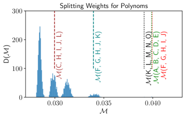
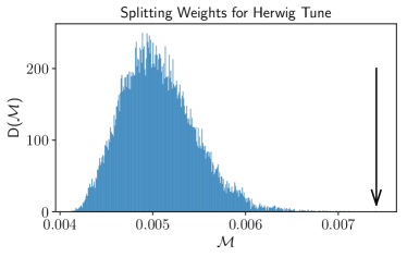
Figure 1: Left: Measure density for all combination vectors according to Equation 4 for ideal conditions of polynomial function, see Section IV.1. Right: Measure density real MCEG tuning. Although the distribution is less resolving, a structure is visible.

The goal of this step is to split up a high dimensional space ($N$ dimensional) into subspaces ($n$ dimensional ), such that the clustered parameters are correlated on the observable level. To achieve this we have to define a quantity $\mathcal{M}$ that can be maximized or minimized to allow the algorithmic treatment. The parameter space we work with is a hyper-rectangle. The observable definitions usually allow to access one dimensional projections. Here, the ’projection’ is the model (implemented in an event generator) at hand.

Two issues directly come to mind: First, we explicitly describe the parameter space $\vec{x}\in[\vec{x}_{\min},\vec{x}_{\max}]$ as a hyper-rectangle rather than a hyper-cube. Some of the parameters could have been measured externally, others are pure model specific. A measure, which allows comparisons between the parameters, needs to be corrected for the initial ranges ($[\vec{x}_{\min},\vec{x}_{\max}]$) defined by the input. To overcome this first problem, we first define $\bar{x_{i}}\in[0,1]$ as the vector normalized to the input range and will describe below how a rescaling is performed to regain the information lost by this normalisation and relate it to the variations on the observables.

The second issue is the generic observable definition. Some of the observable bins are parts of normalized distributions, or even related to other histograms (as is the case for e.g. centrality definitions in heavy ion collisions (Aad et al., 2016)). In other words, the height $y_{O}$ of observables again does not define a good measure to define a generic quantity to minimize. In order to overcome the second problem, we test the observable space with $N_{search}$ random points in the parameter space projected with the model to the observables. The spread for each observable is used to normalize the values to $\bar{y}_{O}\in[0,1]$. Note that an influential parameter can be shadowed by a less important parameter if the latter has a too large initial range. After the normalizations $\bar{x}_{i}$ and $\bar{y}_{O}$ are performed, we use the $N_{search}$-projections to perform linear regression fits for each parameter, and for each observable bin. Due to the normalization of the $y_{O}$-range, the slope is influenced not only by the parameter itself, but also by the spread produced by the other parameters. The reduction of the slope includes a correlation of parameters to other parameters on the observable level. We use the absolute value of the slope to define an averaged gradient or slope-vector $\vec{\mathcal{S}}_{i}$. The sum $\vec{\mathcal{S}_{N}}=\sum_{i}\vec{\mathcal{S}}_{i}$ has in general unequal entries, one for each parameter in the tune. This indicates that the input ranges $[\vec{x}_{\min},\vec{x}_{\max}]$ are of unequal influence on the observables. To correct for this choice and to improve the clustering of parameters with higher correlation, we normalize each $\vec{\mathcal{S}}_{i}$ element-wise with $\vec{\mathcal{S}}_{N}$ to create $\vec{\mathcal{N}}_{i}$,

$$\mathcal{N}^{j}_{i}=\frac{\mathcal{S}^{j}_{i}}{\mathcal{S}^{j}_{N}}\;.$$ (2)

In bin $i$ the component to a parameter of the new vector $\vec{\mathcal{N}}_{i}$ is reduced if other observables are sensitive to the same parameter. The direction of $\vec{\mathcal{N}}_{i}$ indicates the correlation of parameters . We can now use $\vec{\mathcal{N}}_{i}$ to chunk the dimensionality of the problem. Therefore, we calculate the projection for each of the $\vec{\mathcal{N}}_{i}$ on all possible $n$ dimensionnal sub-spaces. This is done by multiplication with combination vectors $\vec{\mathcal{J}}$. Here, $\vec{\mathcal{J}}$ is defined as one of all possible $N$-dimensional vectors with $N-n$ zero entries and $n$ unit entries, where $n$ is again the dimension of the desired sub-space, e.g. $\vec{\mathcal{J}}=(1,0,0,...,1,0,1)$. The sub-space then defines a sub-tune. The sum over all projections,

$$\sum_{i}(\vec{\mathcal{N}}_{i}\cdot\vec{\mathcal{J}})^{k}$$ (3)

can serve as a good measure to be maximized. However, due to the normalization of $\vec{\mathcal{N}}_{i}$ the sum is equal $\vec{\mathcal{J}}$ for $k=1$. For the quantity $\mathcal{M}$ mentioned at the start of the section we use $k=2$ giving,

$$\mathcal{M}(\vec{\mathcal{J}})=\sum_{i}(\vec{\mathcal{N}}_{i}\cdot\vec{\mathcal{J}})^{2}$$ (4)

in order to define the sub-tunes. The maximal $\mathcal{M}(\vec{\mathcal{J}}_{\mathrm{Step1}})$ defines the first of the sub-tunes (Step1). For other steps, we require no overlap between the sub-spaces. This we enforce by requiring a vanishing scalar product $\vec{\mathcal{J}}_{\mathrm{StepN}}\cdot\vec{\mathcal{J}}_{\mathrm{StepM}}$. It is now possible to perform the tuning in the same order as the maximal measures of Equation 4 are found. This would first fix parameters that can modify the description of fewer observables, and then continue to vary parameters that are globally important. In order to first constrain globally important parameters, and then fix specialized parameters, we invert the order of found sub-tunes. We thus have split the dimensionality of the problem, and will ensure, in the following, that observables used in the various sub-tunes are described by the set of influential parameters.

III.2 Assign Weights (Improved Importance)

In the last paragraph, we described how we split up the dimensionality of the full parameter set to allow us to tune subsets, such that parameters with higher correlation on the observable level are tuned simultaneously. To increase the importance of observables that are relevant for the sub-tune, we now try to enhance the relative weight w.r.t. other observables. Here, we use the same vectors $\vec{\mathcal{N}}_{i}$ defined in the last paragraph. These vectors, obtained by linear regression, and normalized to the overall range of observable vectors have the properties, that they point in the parameter space, and, due to the normalization, they correlate the importance of other measured observables to the current bin. We define the weight of the observable bins later used to minimize the $\chi^{2}$ as

$$w_{i}=\frac{(\vec{\mathcal{N}}_{i}\vec{\mathcal{J}}_{\text{Step}})^{2}}{\sum_{j}N^{j}_{i}}\;,$$ (5)

where $\vec{\mathcal{J}}_{\text{Step}}$ is the combinatorial vector defined in Section III.1, corresponding to the sub-tune. This weight has the properties that the multiplication in the numerator increases the weight of the important bins for the sub-tune, while the sum over components of $\vec{N}_{i}$ in the denominator reduces the importance of bins that are equally or more important to other parameters. Note that the $\vec{N}_{i}$ itself are not normalised, only the sum over $i$ is normalised in each component.

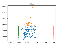
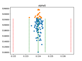
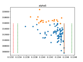
Figure 2: Example of tune results for the $\alpha_{S}(M_{Z})$ value with three iterations from left to right. The points are Goodness of fit (G.o.F.) values given by Professor for various runcombinations (see Sections III.3 and III.4 for details). While the old parameter ranges are given by dashed red lines, the 80% of the best G.o.F. values determine the new green ranges for the next iteration. The lowest G.o.F. value defines the current best tune value that is used for next tune-steps and iterations.

III.3 Run Professor (Tune-Steps)

Before we start the first iteration and step, we perform a second order Professor tune as starting condition, referenced to as BestGuessTune. This is done to reduce the user interference and make use of the sampled points used to determine the spitting of the parameter space and the weight setting described in the previous sections.

After splitting the parameter space and enhancing the weights for important observables for the sub-tunes we use the capability of Professor to tune the parameter space of each step. When a step is performed, we use the Professor result of this and all previous steps to fix the parameters for the following step.

For the individual sub-tunes, we make use of the runcombination method of Professor, to build subsets of the randomly sampled parameter points. This produces modified polynomial interpolations and gives a spread in the $\chi^{2}$ values of the best fit values. We choose the result associated with the best $\chi^{2}$ as the best tune value. To give a measure for the stability of the tune, we choose the runcombinations that give the best $80\%$ of the $\chi^{2}$ values. For those we extract the corresponding parameter range, and add a $20\%$ margin on both sides. To elucidate the effect, an example for the tuning of the strong coupling constant $\alpha_{S}$ is given in Figure 2. Here, the blue points correspond to the $80\%$ best combinations and the green dashed lines give the measure of stability. Diagrams like Figure 2 are automatically produced by the program, for each parameter and tune-step. In Figure 2 three iterations are shown as it is described in the next section.

III.4 Find new ranges and iterate the procedure (Iteration)

The measure of stability defined in the Section III.3 also serves as input for the next iterations. Here we make use of the redefined ranges. An iterative tuning is important, since the first set of parameters has been influenced by the users choices, and a next iteration can have significant impact on the parameter value. For very expensive simulations, at least a retuning of the first step’s parameter space seems desirable. The program is setup such that one can use the output of the first full tune as input for the next iteration.

IV Testing and Findings

Before applying the Autotunes framework to perform a LEP retune of Pythia 8, Herwig 7, and a combination of both in Section V, we test the method under idealized conditions. First, we tune the coefficients of a set of polynomials. The observables used for the tune are constructed from the polynomials for a random choice of coefficients, see Section IV.1. As a second test, we tune the Pythia 8 event generator to pseudo data generated with randomized parameter values. In both scenarios, it is desirable to recover the randomly chosen parameter values that were used to generate the observables.

IV.1 Testing the algorithm under ideal conditions

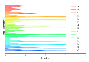
Figure 3: Iterated tuning to polynomial pseudo data using the Autotunes method.

To test the algorithm, we first introduce a simplified and fast generator. We define the projection,

$$\mathcal{O}_{a}=G_{0,a}+G^{i}_{1,a}C_{a}^{ir}p^{r}+G^{ij}_{2,a}C_{a}^{ir}p^{r}p^{j}+G^{ijk}_{3,a}C_{a}^{ir}p^{r}p^{j}p^{k}+G^{ijkl}_{4,a}C_{a}^{ir}p^{r}p^{j}p^{k}p^{l}\;,$$ (6)

with $m$-dimensional tensors $G^{\cdots}_{m,a}$, correlation matrices $C_{a}^{ir}$, and parameter points $p^{i}$. Upper indices sum over the parameter dimensions. We fill $G^{\cdots}_{m}$ with random numbers and use $C_{a}^{ir}$ to correlate subsets of parameters. Here $C_{a}^{ir}$ is a diagonal matrix with constant entries $k>1$ if the bin $a$ should be enhanced for this parameter $i$ and one if not. By building ranges, we can define enhanced parameter sets. As an example, we use a $d=15$ dimensional parameter space, and correlate the parameter in combinations as [A,B,C,D,E], [F,G,H,I,J] and [K,L,M,N,O]. Under these ideal conditions, we search for the correlations with the procedure described in Section III.1 . In Figure 1(left), the weights for the parameter correlations are shown. The ideal combinations defined above create the highest weights, and would therefore be detected as correlated by the algorithm. In a real life MCEG tune the correlations are much less pronounced. In the right panel of Figure 1, we show the weight distribution for the example of the Herwig 7 tune described in Section V.2.1. Once the correlated combinations are found, the algorithm continues with the procedure described in Sections III.3 and III.2. As the result of each full tune serving as input to a next iteration, it is possible to visualize the outcome as a function of tune iterations. Figure 3 shows this visualisation as produced by the program. Each parameter (A-O) is normalised to the initial range, and plotted with an offset. In this example, it is possible to show the input values of the pseudo data with dashed lines. This is not possible when tuning is performed to real data. As Professor is very well capable of finding polynomial behaviour, the parameter point that the method aims to find is already well constrained after the first iteration. However, next iterations still improve the result. This may be seen for example in the third and last line.

The procedure to split the parameter space into smaller subsets, and to assign weights can suffer from numerical and statistical noise if we consider many observables. In Appendix A, we discuss the range dependence and show that the weight distributions are fairly stable if the same parameters are found to be correlated. It is further possible to ask for weights, if all parameters should be tuned independently. From the tuning perspective this seems an unnecessary feature, but can help to find observables that are likely influenced by a model parameter, e.g it is possible to identify the range of bins where the bottom mass has influence in jet rates.

IV.2 Tuning Pythia 8 to pseudo data

As a second test of our method, we use Pythia 8 to generate pseudo data for a random choice of 18 relevant parameter values. We then use three different methods to tune Pythia 8 to this set of pseudo data, and try to recover the true parameters. In all methods, we divide the tuning into three sub-tunes. The first method is a random selection of parameters out of the full set, with unit weights on all observables. In the second method, we choose the simultaneously tuned parameters based on physical motivation, but still use unit weights on all observables. Finally, we use the Autotunes method to divide the parameters into steps, and automatically set weights as described in Section III.

The choice of parameters used in the physically motivated method is given in Table 1. The first step collects parameters that have a significant influence on many observables, combining shower and Pythia 8 string parameters. The second step gathers additional properties of the string model (Andersson et al., 1983; Sjöstrand, 1984), focusing on the flavor composition. The last step then tunes the ratio of vector-to-pseudoscalar meson production.

Step 1	Step 2	Step 3
TimeShower:alphaSvalue	StringFlav:probStoUD	StringFlav:mesonUDvector
TimeShower:pTmin	StringFlav:probQQtoQ	StringFlav:mesonSvector
StringZ:aLund	StringFlav:probSQtoQQ	StringFlav:mesonCvector
StringZ:bLund	StringFlav:probQQ1toQQ0	StringFlav:mesonBvector
StringPT:Sigma	StringFlav:etaSup
StringZ:aExtraSQuark	StringFlav:etaPrimeSup
StringZ:aExtraDiquark	StringFlav:popcornRate

Table 1: Parameters chosen to be tuned simultaneously in the physics motivated tuning approach.

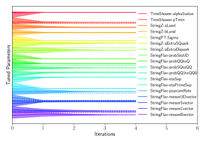
(a) Iterated Pythia 8 pseudo data tune with random choice of parameter subset.

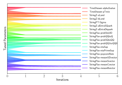
(b) Iterated Pythia 8 pseudo data tune with physically motivated choice of parameters.

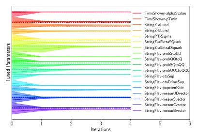
(c) Iterated Pythia 8 pseudo data tune using the Autotunes method.

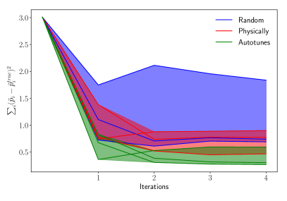
(d) Comparison in summed deviation from true parameters. Iterating the Autotunes approach leads to better agreement with initially chosen parameters.

Figure 4: Parameter development as a function of tune iterations. The dashed lines in Figures 4(a), 4(b) and 4(c) shows the true parameter point that was used to produce the pseudo data. The uncertainty bands are given by 80% of the best fit values in the Professor run-combinations and an additional 20% margin. In Figure 4(d) we compare the the summed deviation for three distinct tunes for the random, physically motivated and Autotunes method.

The results of the three tuning approaches that aim to recover the Pythia 8 pseudo data parameters are shown in Figures 4(a), 4(b), 4(c) and 4(d). None of the approaches is capable of exactly recovering all of the original parameter values. This suggests that close-by points in parameter space are well suited to reproduce the pseudo data observable distributions. However, the iterated Autotunes method improves the agreement of the recovered parameters by avoiding large mismatches. In the physically motivated and random approaches, there is a certain chance that parameters are strongly constrained by observables that also depend on other parameters. If these are not identified and included in the same sub-tune, both parameters get constrained. Thus, the optimal configuration is not necessarily recovered. By iteratively identifying such sets of parameters, the Autotunes method avoids these mismatches.

Figure 4(d) shows the summed, squared and normalized deviation of the recovered to the true parameter values. Each approach is performed three times to access the stability of the results. The random approach uses random combinations of parameters for the tuning steps, so we see a wide spread of results. The iterative tuning using our fixed physically motivated parameter choice is more reliable, showing a lower spread and better results. The Autotunes method leads to the best agreement with the original parameters. More stable results in the physically motivated and the Autotunes method could be achieved by using higher statistics for both the event generation and the sampling. We see that in the physically motivated and the Autotunes approach, a second tuning iteration affects the results, mostly – but not necessarily – improving the parameter agreement. Further iterations have a minor impact.

V Results

We use the Autotunes framework to perform five distinct tunes to LEP observables. We provide the list of analyses in the additional material with the arXiv upload. To this point we do not weight the LEP observables, but make use of the sub-tune weights described in Section III.2 . The tunes make use of the default hadronisation models of the event generators Herwig 7 and Pythia 8. We further present a new tune of the Herwig 7 event generator interfaced to the Pythia 8 string hadronisation model. The details of the simulations can be found in the following sections. The results are presented in Table 2 and Table 3, listing default values, tuning ranges of the parameters, as well as the tuning results using the Autotunes method.

V.1 Retuning of Pythia 8

The tune of Pythia 8.235 is performed by using LEP data. We use Pythia 8’s standard configuration as described in the manual, including a one-loop running of $\alpha_{\text{s}}$ in the parton shower. The tuned parameters, initial ranges and tune results are given in Table 2 in Appendix B.

The given ranges on the tune results, obtained from the variation of the optimal tune in different run combinations, can be interpreted as a measure of the stability of the best tune. A wide range suggests that different configurations give tunes of similar $\chi^{2}$. The extraction of the strong coupling $\alpha_{s}$ is the most stable result in the tune. The modification of the longitudinal lightcone fraction distribution in the string fragmentation model for strange quarks (StringZ:aExtraSQuark) is very loosely constrained, suggesting that the data that is employed in the tune is not suitable to extract this parameter.

We tune 18 parameters in three sets of six parameters each. In the Pythia 8 tune, the parton shower cutoff pTmin is surprisingly loosely constrained. Checking the combinations of parameters that the Autotunes method chooses, we note that pTmin is found to be correlated with the string fragmentation parameters aLund and bLund in every iteration, which are also rather loosely constrained. This suggests that different choices for these three parameters can provide tunes of similar $\chi^{2}$.

V.2 Retuning of Herwig 7

As another real life example we tune the Herwig 7 event generator to LEP data. Here the tune is based upon version Herwig 7.1.4 and ThePEG 2.1.4. We perform two tunes – cluster and string model – for both showers, the QTilde shower (Gieseke et al., 2003) and the dipole shower (Platzer and Gieseke, 2011). For the presented tunes we do not employ the CMW scheme (Catani et al., 1991), but keep the $\alpha_{S}(M_{Z})$ value a free parameter. This results in the enhanced value compared to the world average (Tanabashi et al., 2018).

V.2.1 Tuning Herwig 7 with cluster model

We retune the cluster-model with a 22 dimensional parameter space. Here, we require tree sub-tunes and performed four iterations. The results are listed in Appendix B. Comparing the results, we note that the method is in general able to find values outside of the given initial parameter ranges, see e.g. the $\alpha_{S}(M_{Z})$ or the nominal $b$-mass. This can be caused by Professor interpolation outside the given bounds or in the determination of the new ranges for the next iteration. Apart from the parameters that influence the cluster fission process of heavy clusters involving charm quarks (ClPowCharm and PSplitCharm), the parameters are comparable between the two shower models. Further in the cluster-model, the fission parameters are correlated. It is reasonable to assume possible local minima in the $\chi^{2}$ measure.

V.2.2 Tuning Herwig 7 with Pythia 8 Strings

The usual setup of the event generators are genuinely well-tuned and even though the tests of Section IV allow the conclusion that relatively arbitrary starting points lead to similar results, ignoring the previous knowledge completely seems undesirable. To create a real live example and further allow useful future studies we employed the fact that the C++ version of the Ariadne shower but also the Herwig 7 event generator is based on ThePEG. Furthermore with minor modifications, the unpublished interface between ThePEG and Pythia 8 (called TheP8I, written by L. Lönnblad), allowed the internal use of Pythia 8-stings with Herwig 7 events. Since no tuning for this setup was attempted before the starting conditions needed to be chosen with less bias compared to the other results of this section.

When we compare the values received for the Herwig 7 showers to the Pythia 8 shower, we note a comparably large value for the Pythia 8 $\alpha_{S}$ value. In contrast, the cutoff in the transverse momentum in Pythia 8 is rather small. The reason for this contradicting behaviour can be found in the order at which the two codes evaluate the running of the strong coupling. While Herwig 7 chooses an NLO running, Pythia 8 evolves $\alpha_{S}$ with LO running, and therefore suppresses the radiation for low energies. Even though the shower models are rather different, the difference in the response in the best fit values of the parameters are moderate. Less constrained parameters like the popcornRate, which influences part of the baryon production or the additional strange quark parameter aExtraSQuark show a corresponding large uncertainty. It can be concluded that the data used for tuning is hardly constraining these parameters.

VI Conclusion and Outlook

We presented an algorithm that allows a semi-automatic Monte Carlo Event generator tuning of high dimensional parameter space. Here, we motivated and described how the parameter space can be split into sub-spaces, based on the projections to and variations in the observable space. We then assigned increased weights when we perform the sub-tunes, such that influential observables are highlighted. It is then possible to use the output of any tune step as starting conditions for next steps. Therefore the procedure is iterative. In ideal conditions, we performed tests to check that the algorithm finds correlated parameters and showed in realistic environment that pseudo data could be reproduced better by the algorithm than by random or physically motivated tunes. As real life examples we tuned the Pythia 8 and Herwig 7 showers with their standard hadronisations models and modified the Herwig 7 generator to allow consistent hadronisation with the Pythia 8’s Lund String model.

The method allows to perform tuning with far less human interaction. It also allows different models to be tuned with a similar bias. Such tunes can then be used to identify mismodelling, with the assurance that the origin of the difference in data description is less likely part of a better or worse tuning.

At the current stage we did not assign weights or uncertainties other than the sub-tune weights and the uncertainties given by the experimental collaborations. We note that the difference between higher multiplicity merged simulations to the pure parton shower simulations can serve as an excellent reduction weight to suppress observables influenced by higher order calculations. However, the investigation of such procedures goes beyond the scope of this paper and will be subject to future work. Further, we did not address the third point of the mentioned restrictions in Section II.1 that describes over-represented data. We postpone such studies, that include clustering of slope-vectors to reduce such an influence, to future work.

Appendix A Range dependence

The algorithm to split the dimensions and to assign weights to sub-tunes is constructed such that correlations should still be found when the parameter ranges are varied. This is not always possible if the parameter ranges are strongly modified. It is possible that the slope vectors, that are evaluated by averaging over the full $n-1$ (other) dimensions, are modified by the newly defined initial ranges. It is even possible that the range of other parameters influence the slope as the spread modifies the normalisation. In order to show such behaviour (and also to illustrate the weight distributions), we choose three different setups for the event generator Herwig 7. We choose $d=4$ and try to split the dimensions in half. Here we choose the parameters and initial ranges as,

Parameter	Setup 1	Setup 2	Setup 3
$\alpha_{S}(M_{Z})$	0.12 – 0.13	0.124 – 0.126	0.12 – 0.13
$Cl_{\max}^{light}$	2.0 – 3.0	2.4 – 2.6	2.4 – 2.6
$p^{T}_{\min}$	0.7 – 0.9	0.7 – 0.9	0.78 – 0.82
$g_{CM}$	0.7 – 0.9	0.7 – 0.9	0.7 – 0.9

The result for the parameter grouping and the weight distributions are depicted in Figure 5. While the algorithm to split the parameter space in setup 1 and setup 2 such that $Cl_{\max}^{Light}$ and $p^{T}_{\min}$ should be tuned in the first step and then $\alpha_{S}(M_{Z})$ and $g_{CM}$ in a second step, the modification to the initial ranges has the effect that the algorithm favours the pairing ($Cl_{\max}^{Light}$ , $g_{CM}$) and ($\alpha_{S}$ , $p^{T}_{\min}$) for steps 1 and 2 for setup 3.

While it is possible that by changing the initial ranges the pairing flips and other parameter groups are found, the fact that neighbouring bins have a similar behaviour supports the concept of meaningful weight distributions. It would be possible to correlate neighbouring bins or introduce a smoothing algorithm to make the weights more stable but such a modification can be introduced once issues with the current algorithm appear.

In principle, it is possible to visualize for each parameter the weights of the sub-tune choice that we want. This choice can help to identify observables that are influential for individual parameters, and give insights in unexpected behaviours. Already from the weight distributions shown in Figure 5, we can deduce that $p^{T}_{\min}$ is of great importance for the transverse momentum out-of-plane, see upper left panel. Further modifications of the constituent mass of the gluon $g_{CM}$ will influence the difference in the hemisphere masses, see lower right panel.

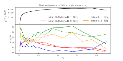
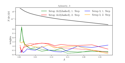
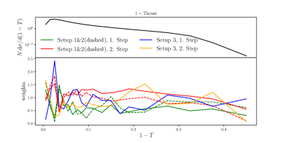
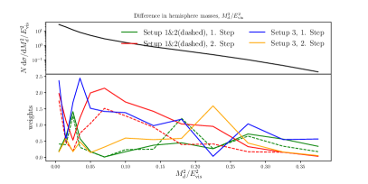
Figure 5: Weight distributions for subsets of parameter pairs as described in Appendix A. The upper panels show the measured data points and the lower panels show the weights assigned. A clear distinction between more and less important sets is visible. The dashed lines correspond to Setup 2, which gives a same grouping of parameters as Setup 1. .

Appendix B Tune Results

In Table 2 and Table 3 we list the results of the Herwig 7 and Pythia 8 tunes with the standard hadronisation. For Herwig 7 we also list a tune for the Lund string model. The results are discussed in Section V.

Parameter	Def.	range	Pythia 8 tune	H7+$\tilde{Q}$+Str.	H7+Dip.+Str.
alphaSvalue	$0.1365$	$0.125-0.14$	$0.13699_{-0.00057}^{+0.00019}$	$0.1289_{-0.0004}^{+0.0011}$	$0.13229_{-0.00015}^{+0.00083}$
pTmin	$0.5$	$0.4-0.8$	$0.49_{-0.16}^{+0.05}$	$0.993_{-0.004}^{+0.010}$	$0.990_{-0.004}^{+0.020}$
SZ-aLund	$0.68$	$0.5-0.8$	$0.71_{-0.24}^{+0.07}$	$0.60_{-0.19}^{+0.13}$	$0.84_{-0.16}^{+0.03}$
SZ-bLund	$0.98$	$0.7-1.3$	$1.11_{-0.23}^{+0.11}$	$0.78_{-0.19}^{+0.18}$	$1.00_{-0.20}^{+0.04}$
StringPT-Sigma	$0.335$	$0.3-0.4$	$0.3011_{-0.0010}^{+0.0020}$	$0.3008_{-0.0022}^{+0.0006}$	$0.29876_{-0.00022}^{+0.00122}$
SZ-aExtraSQuark	$0.0$	$0.0-0.5$	$0.04_{-0.05}^{+0.60}$	$0.08_{-0.08}^{+0.26}$	$0.22_{-0.22}^{+0.37}$
SZ-aExtraDiquark	$0.97$	$0.8-1.2$	$1.19_{-0.18}^{+0.06}$	$1.1_{-0.6}^{+0.3}$	$1.02_{-0.18}^{+0.38}$
SF-probStoUD	$0.217$	$0.1-0.3$	$0.196_{-0.004}^{+0.010}$	$0.2186_{-0.0103}^{+0.0018}$	$0.1979_{-0.0066}^{+0.0016}$
SF-probQQtoQ	$0.081$	$0.0-0.2$	$0.0828_{-0.0024}^{+0.0011}$	$0.0821_{-0.0032}^{+0.0010}$	$0.0856_{-0.0039}^{+0.0007}$
SF-probSQtoQQ	$0.915$	$0.8-1.0$	$0.98_{-0.05}^{+0.09}$	$0.748_{-0.029}^{+0.091}$	$0.797_{-0.009}^{+0.004}$
SF-probQQ1toQQ0	$0.0275$	$0.0-0.1$	$0.033_{-0.011}^{+0.003}$	$0.024_{-0.006}^{+0.008}$	$0.023_{-0.003}^{+0.007}$
SF-etaSup	$0.6$	$0.4-0.8$	$0.644_{-0.018}^{+0.034}$	$0.800_{-0.036}^{+0.012}$	$0.7976_{-0.0068}^{+0.0018}$
SF-etaPrimeSup	$0.12$	$0.0-0.3$	$0.1095_{-0.0016}^{+0.0054}$	$0.1027_{-0.0022}^{+0.0115}$	$0.100_{-0.008}^{+0.017}$
SF-popcornRate	$0.5$	$0.4-0.6$	$0.31_{-0.05}^{+0.27}$	$0.63_{-0.36}^{+0.12}$	$0.51_{-0.17}^{+0.08}$
SF-mesonUDvector	$0.5$	$0.3-0.7$	$0.527_{-0.023}^{+0.027}$	$0.459_{-0.008}^{+0.031}$	$0.473_{-0.047}^{+0.009}$
SF-mesonSvector	$0.55$	$0.35-0.75$	$0.53_{-0.08}^{+0.07}$	$0.55_{-0.05}^{+0.07}$	$0.581_{-0.044}^{+0.018}$
SF-mesonCvector	$0.88$	$0.7-1.1$	$0.874_{-0.024}^{+0.021}$	$1.10_{-0.22}^{+0.08}$	$0.72_{-0.08}^{+0.13}$
SF-mesonBvector	$2.2$	$2.0-2.4$	$2.24_{-0.20}^{+0.16}$	$2.34_{-0.50}^{+0.09}$	$2.31_{-0.44}^{+0.27}$

Table 2: Tuned Pythia 8 parameters with default values, initial ranges for the tune, and the Autotunes result. See (Sjöstrand et al., 2006, 2015) for details on the parameters. (SF=StringFlav,SZ=StringZ)

Parameter	Def.	Range	H7+Dip.+Cluster	H7+$\tilde{Q}$+ Cluster
alphaS	0.126234	0.12 – 0.13	$0.13008_{-0.00061}^{+0.00013}$	$0.12455_{-0.00118}^{+0.00020}$
gConstituentMass	0.95	0.7 – 1.1	$0.83_{-0.07}^{+0.16}$	$1.0045_{-0.0006}^{+0.0028}$
EMpTmin	1.2228	0.8 – 1.4	$1.204_{-0.033}^{+0.010}$	$1.068_{-0.020}^{+0.004}$
SPpTmin	1.2228	0.8 – 1.4	$1.204_{-0.033}^{+0.010}$	$1.22_{-0.74}^{+0.27}$
bNominalMass	4.2	4.0 – 4.7	$4.76_{-0.21}^{+0.04}$	$4.2_{-0.5}^{+0.9}$
bConstituentMass	5.	4.0 – 4.7	$4.01_{-0.13}^{+0.22}$	$4.03_{-0.15}^{+0.17}$
DecWt	0.62	0.5 – 0.9	$0.59_{-0.05}^{+0.10}$	$0.61_{-0.04}^{+0.05}$
SngWt	0.74	0.5 – 0.9	$0.86_{-0.11}^{+0.18}$	$0.80_{-0.37}^{+0.14}$
ClSmrLight	0.78	0.5 – 1.0	$0.59_{-0.08}^{+0.05}$	$0.437_{-0.013}^{+0.041}$
ClSmrCharm	0.	0.0 – 0.2	$0.24_{-0.21}^{+0.04}$	$0.18_{-0.18}^{+0.04}$
ClSmrBottom	0.0204	0.0 – 0.1	$0.100_{-0.044}^{+0.019}$	$0.088_{-0.033}^{+0.018}$
ClMaxLight	3.00254	3.0 – 5.0	$3.18_{-0.22}^{+0.11}$	$3.13_{-0.14}^{+0.08}$
ClMaxCharm	3.63822	3.0 – 5.0	$3.34_{-0.07}^{+0.25}$	$3.68_{-0.07}^{+0.28}$
ClMaxBottom	3.911	3.0 – 5.0	$4.4_{-0.6}^{+1.6}$	$4.9_{-2.9}^{+0.9}$
ClPowLight	1.42426	1.0 – 1.8	$1.85_{-0.58}^{+0.24}$	$1.36_{-0.03}^{+0.15}$
ClPowCharm	2.33186	1.5 – 3.0	$1.89_{-0.29}^{+1.71}$	$3.1_{-1.5}^{+0.4}$
ClPowBottom	0.6375	0.4 – 0.8	$0.638_{-0.018}^{+0.104}$	$0.80_{-0.23}^{+0.04}$
PSplitLight	0.847541	0.0 – 1.5	$0.8747_{-0.0007}^{+0.0041}$	$0.935_{-0.018}^{+0.035}$
PSplitCharm	1.23399	0.0 – 1.5	$0.637_{-0.028}^{+0.164}$	$1.20_{-0.66}^{+0.11}$
PSplitBottom	0.5306	0.0 – 1.5	$0.599_{-0.113}^{+0.019}$	$0.69_{-0.12}^{+0.12}$
SingleHadronLimitCharm	0.0	0.0 – 0.5	$0.0015_{-0.0015}^{+0.0156}$	$0.0012_{-0.0012}^{+0.0061}$
SingleHadronLimitBottom	0.0	0.0 – 0.5	$0.08_{-0.09}^{+0.12}$	$0.015_{-0.016}^{+0.009}$

Table 3: Result of the retuning of the Herwig 7 event generator employing the default hadronisation model (cluster model). The 22 dimensional parameter space was tuned with three sub-tunes and three iterations. Shown are the default values (corresponding to the Qtilde shower tune) as well as the parameter range and the tuning result for both showers.

References

- Buckley et al. (2011) A. Buckley et al., Phys. Rept. 504, 145 (2011), eprint 1101.2599.
- Bähr et al. (2008) M. Bähr et al., Eur. Phys. J. C58, 639 (2008), eprint 0803.0883.
- Bellm et al. (2016a) J. Bellm et al., Eur. Phys. J. C76, 196 (2016a), eprint 1512.01178.
- Platzer and Gieseke (2012) S. Platzer and S. Gieseke, Eur. Phys. J. C72, 2187 (2012), eprint 1109.6256.
- Bellm et al. (2017) J. Bellm et al. (2017), eprint 1705.06919.
- Gleisberg et al. (2004) T. Gleisberg, S. Höche, F. Krauss, A. Schalicke, S. Schumann, and J.-C. Winter, JHEP 02, 056 (2004), eprint hep-ph/0311263.
- Sjöstrand et al. (2006) T. Sjöstrand, S. Mrenna, and P. Z. Skands, JHEP 05, 026 (2006), eprint hep-ph/0603175.
- Sjöstrand et al. (2015) T. Sjöstrand, S. Ask, J. R. Christiansen, R. Corke, N. Desai, P. Ilten, S. Mrenna, S. Prestel, C. O. Rasmussen, and P. Z. Skands, Comput. Phys. Commun. 191, 159 (2015), eprint 1410.3012.
- Reichelt et al. (2017) D. Reichelt, P. Richardson, and A. Siodmok, Eur. Phys. J. C77, 876 (2017), eprint 1708.01491.
- Gieseke et al. (2018) S. Gieseke, P. Kirchgaeßer, and S. Plätzer, Eur. Phys. J. C78, 99 (2018), eprint 1710.10906.
- Höche and Prestel (2017) S. Höche and S. Prestel, Phys. Rev. D96, 074017 (2017), eprint 1705.00742.
- Höche et al. (2017) S. Höche, F. Krauss, and S. Prestel, JHEP 10, 093 (2017), eprint 1705.00982.
- Bellm (2018) J. Bellm, Eur. Phys. J. C78, 601 (2018), eprint 1801.06113.
- Duncan and Kirchgaeßer (2019) C. B. Duncan and P. Kirchgaeßer, Eur. Phys. J. C79, 61 (2019), eprint 1811.10336.
- Dulat et al. (2018) F. Dulat, S. Höche, and S. Prestel, Phys. Rev. D98, 074013 (2018), eprint 1805.03757.
- Bewick et al. (2019) G. Bewick, S. Ferrario Ravasio, P. Richardson, and M. H. Seymour (2019), eprint 1904.11866.
- Barate et al. (1998) R. Barate et al. (ALEPH), Phys. Rept. 294, 1 (1998).
- Hamacher and Weierstall (1995) K. Hamacher and M. Weierstall (DELPHI) (1995), eprint hep-ex/9511011.
- Abreu et al. (1996) P. Abreu et al. (DELPHI), Z. Phys. C73, 11 (1996).
- Skands (2009) P. Z. Skands, in Proceedings, 1st International Workshop on Multiple Partonic Interactions at the LHC (MPI08): Perugia, Italy, October 27-31, 2008 (2009), pp. 284–297, eprint 0905.3418, URL http://lss.fnal.gov/cgi-bin/find_paper.pl?conf-09-113.
- Buckley et al. (2010) A. Buckley, H. Hoeth, H. Lacker, H. Schulz, and J. E. von Seggern, Eur. Phys. J. C65, 331 (2010), eprint 0907.2973.
- Skands et al. (2014) P. Skands, S. Carrazza, and J. Rojo, Eur. Phys. J. C74, 3024 (2014), eprint 1404.5630.
- Khachatryan et al. (2016) V. Khachatryan et al. (CMS), Eur. Phys. J. C76, 155 (2016), eprint 1512.00815.
- Ilten et al. (2017) P. Ilten, M. Williams, and Y. Yang, JINST 12, P04028 (2017), eprint 1610.08328.
- Buckley and Schulz (2018) A. Buckley and H. Schulz, Adv. Ser. Direct. High Energy Phys. 29, 281 (2018), eprint 1806.11182.
- Bellm et al. (2016b) J. Bellm, S. Plätzer, P. Richardson, A. Siódmok, and S. Webster, Phys. Rev. D94, 034028 (2016b), eprint 1605.08256.
- Mrenna and Skands (2016) S. Mrenna and P. Skands, Phys. Rev. D94, 074005 (2016), eprint 1605.08352.
- Bothmann et al. (2016) E. Bothmann, M. Schönherr, and S. Schumann, Eur. Phys. J. C76, 590 (2016), eprint 1606.08753.
- Bothmann and Debbio (2019) E. Bothmann and L. Debbio, JHEP 01, 033 (2019), eprint 1808.07802.
- Andreassen and Nachman (2019) A. Andreassen and B. Nachman (2019), eprint 1907.08209.
- Maguire et al. (2017) E. Maguire, L. Heinrich, and G. Watt, J. Phys. Conf. Ser. 898, 102006 (2017), eprint 1704.05473.
- Buckley et al. (2013) A. Buckley, J. Butterworth, L. Lonnblad, D. Grellscheid, H. Hoeth, J. Monk, H. Schulz, and F. Siegert, Comput. Phys. Commun. 184, 2803 (2013), eprint 1003.0694.
- Andersson et al. (1983) B. Andersson, G. Gustafson, G. Ingelman, and T. Sjöstrand, Phys. Rept. 97, 31 (1983).
- Sjöstrand (1984) T. Sjöstrand, Nucl. Phys. B248, 469 (1984).
- Aad et al. (2016) G. Aad et al. (ATLAS), Eur. Phys. J. C76, 199 (2016), eprint 1508.00848.
- Gieseke et al. (2003) S. Gieseke, P. Stephens, and B. Webber, JHEP 12, 045 (2003), eprint hep-ph/0310083.
- Platzer and Gieseke (2011) S. Platzer and S. Gieseke, JHEP 01, 024 (2011), eprint 0909.5593.
- Catani et al. (1991) S. Catani, B. R. Webber, and G. Marchesini, Nucl. Phys. B349, 635 (1991).
- Tanabashi et al. (2018) M. Tanabashi et al. (Particle Data Group), Phys. Rev. D98, 030001 (2018).