Universality of lower hybrid waves at Earth’s magnetopause

Abstract

Waves around the lower hybrid frequency are frequently observed at Earth’s magnetopause, and readily reach very large amplitudes. Determining the properties of lower hybrid waves is crucial because they are thought to contribute to electron and ion heating, cross-field particle diffusion, anomalous resistivity, and energy transfer between electrons and ions. All these processes could play an important role in magnetic reconnection at the magnetopause and the evolution of the boundary layer. In this paper, the properties of lower hybrid waves at Earth’s magnetopause are investigated using the Magnetospheric Multiscale (MMS) mission. For the first time, the properties of the waves are investigated using fields and direct particle measurements. The highest-resolution electron moments resolve the velocity and density fluctuations of lower hybrid waves, confirming that electrons remain approximately frozen in at lower hybrid wave frequencies. Using fields and particle moments the dispersion relation is constructed and the wave-normal angle is estimated to be close to $90^{\circ}$ to the background magnetic field. The waves are shown to have a finite parallel wave vector, suggesting that they can interact with parallel propagating electrons. The observed wave properties are shown to agree with theoretical predictions, the previously used single-spacecraft method, and four-spacecraft timing analyses. These results show that single-spacecraft methods can accurately determine lower hybrid wave properties.

JGR-Space Physics

Swedish Institute of Space Physics, Uppsala, Sweden. Birkeland Centre for Space Science, Department of Physics and Technology, University of Bergen, Bergen, Norway. Space and Plasma Physics, School of Electrical Engineering and Computer Science, KTH Royal Institute of Technology, Stockholm, Sweden. IREAP, University of Maryland, College Park, Maryland, USA. Department of Physics, University of Wisconsin–Madison, Madison, Wisconsin 53706, USA. Institute of Space Science and Technology, Nanchang University, Nanchang 330031, People’s Republic of China. Laboratoire de Physique des Plasmas, CNRS/Ecole Polytechnique/Sorbonne Université/Univ. Paris Sud/Observatoire de Paris, Paris, France. Department of Physics and Astronomy, Rice University, Houston, TX, USA. IRAP, Université de Toulouse, CNRS, CNES, UPS, Toulouse, France. NASA Goddard Space Flight Center, Greenbelt, MD, USA. Department of Astronomy, University of Maryland, College Park, MD, USA. Southwest Research Institute, San Antonio, TX, USA. Laboratory of Atmospheric and Space Physics, University of Colorado, Boulder, CO, USA.

D. B. Grahamdgraham@irfu.se

1: The velocity and density fluctuations of lower hybrid waves are resolved, showing that electrons remain approximately frozen in.

2: Lower hybrid wave dispersion relation and wave-normal angle are computed from fields and particle measurements.

3: Single- and multi-spacecraft methods yield consistent lower hybrid wave properties, confirming the accuracy of single-spacecraft methods.

1 Introduction

Lower hybrid drift waves are waves that develop at frequencies between the ion and electron gyrofrequencies, with wavelengths between the electron and ion thermal gyroradii Krall and Liewer (1971); Davidson et al. (1977). Under these conditions the electrons remain approximately magnetized, while the ions are unmagnetized. In general, lower hybrid waves are treated in the electrostatic approximation, typically assuming a plasma beta less than unity Krall and Liewer (1971); Davidson and Gladd (1975). Both observations and simulations show that these waves have properties consistent with predictions of the electrostatic lower hybrid drift instability, namely wave numbers of $k\rho_{e}\sim 0.5$ and frequency $\omega\lesssim\omega_{LH}$, where $\rho_{e}$ is the electron thermal gyroradius and $\omega_{LH}$ is the angular lower hybrid frequency Graham et al. (2017a); Khotyaintsev et al. (2016); Le et al. (2017, 2018). Although the lower hybrid wave properties are consistent with electrostatic predictions, the waves are generally not electrostatic in the sense that the fluctuating magnetic fields $\delta{\bf B}$ are not zero. Magnetic field fluctuations develop due to the currents associated with waves Norgren et al. (2012). Both observations and simulations show that these magnetic field fluctuations are often primarily in the direction parallel to the background magnetic field, and are frequently observed at Earth’s magnetopause Bale et al. (2002); Graham et al. (2016a, 2017a).

Lower hybrid waves are thought to play an important role in magnetic reconnection. Lower hybrid waves can be of particular importance because they can contribute to anomalous resistivity Davidson and Gladd (1975); Huba et al. (1977); Silin et al. (2005), heat electrons and ions McBride et al. (1972); Cairns and McMillan (2005), transfer energy between electrons and ions, and produce cross-field particle diffusion Treumann et al. (1991); Vaivads et al. (2004); Graham et al. (2017a). In magnetopause reconnection lower hybrid waves are found at the density gradient on the magnetospheric side of the X line Graham et al. (2016a, 2017a); Khotyaintsev et al. (2016), where the stagnation point is expected to occur Cassak and Shay (2007). Therefore, lower hybrid waves could potentially play a significant role in reconnection at Earth’s magnetopause. This can modify the predictions of two-dimensional simulations of magnetic reconnection, which suppress lower hybrid waves. More generally, plasma boundaries, regardless of whether or not magnetic reconnection is occurring, can be unstable to lower hybrid waves, so it is important to characterize the observed lower hybrid waves and determine what effects they have on electrons and ions, and how they can modify the boundaries.

During the first magnetopause phase of the Magnetospheric Multiscale (MMS) mission the four spacecraft reached separations as small as $\sim 15\,\mathrm{km}$. These separations were either comparable to or larger than the wavelengths of lower hybrid waves $\sim 10\,\mathrm{km}$ at Earth’s magnetopause Graham et al. (2016a, 2017a). Therefore, because of the typically broadband (and possibly turbulent) nature of the waves, timing analysis could not be used to accurately determine the wave properties, such as phase speed, propagation direction, wavelength, and wave potential. These properties were determined using a single-spacecraft method Norgren et al. (2012); Graham et al. (2016a); Khotyaintsev et al. (2016); Graham et al. (2017a). However, during the MMS’s second magnetopause phase beginning in September 2016, the spacecraft separations were as small as $\sim 5\,\mathrm{km}$. These separations are below the typical wavelength of the quasi-electrostatic lower hybrid wave and thus enable the lower hybrid wave properties to be determined using four-spacecraft timing analyses for the first time. In addition, it is possible with MMS to measure the electron distributions and moments at $7.5$ ms resolution (corresponding to a Nyquist frequency of $67$  Hz) Rager et al. (2018), which is often sufficient to resolve the lower hybrid frequency at Earth’s magnetopause.

In this paper we investigate the properties and generation mechanisms of lower hybrid waves at Earth’s magnetopause. For the first time we investigate the lower hybrid waves using direct particle measurements and show that their properties are consistent with theoretical predictions. We compare the single-spacecraft method developed in Norgren et al. (2012) and single spacecraft methods developed in this paper, based on the measured electron moments with four-spacecraft timing to determine the properties of the lower hybrid waves. When the spacecraft separations are sufficiently small to enable multi-spacecraft timing to be applied, the results show good agreement with the single-spacecraft methods, confirming their accuracy. Lower hybrid waves produced by magnetosheath ions entering the magnetosphere via the finite gyroradius effect are shown to be consistent with generation by the modified two-stream instability McBride et al. (1972); Wu et al. (1983). We show that lower hybrid waves are generated in the ion diffusion region of magnetopause reconnection and are driven by a large ${\bf E}\times{\bf B}$ electron drift and a smaller electron diamagnetic drift.

This paper is organized as follows: In section 2 we review the properties of lower hybrid waves based on cold plasma theory. In section 3 we introduce the data used. In sections 4 and 5 we investigate in detail the lower hybrid waves observed at two magnetopause crossings observed on 28 November 2016 and 14 December 2015. Section 6 contains the discussion and the conclusions are stated in section 7.

2 Lower hybrid wave properties

In this section we review the fields and particle properties of lower hybrid waves predicted from cold plasma theory. The derivation of the cold plasma dispersion equation and the wave properties are well known and derived in several plasma physics textbooks (e.g., Stix, 1962; Swanson, 1989), so are not repeated here. Electric fields are calculated from the dielectric tensor, magnetic fields are computed from Faraday’s law, electron and ion velocities are calculated from the momentum equation, and density perturbations are calculated from the continuity equation. Lower hybrid waves are found for $k_{\perp}\gg k_{\parallel}$ on the whistler dispersion surface André (1985), where $k_{\parallel}$ and $k_{\perp}$ are the wave numbers parallel and perpendicular to the background magnetic field ${\bf B}$. At the magnetopause $f_{pe}/f_{ce}>1$, where $f_{pe}$ is the electron plasma frequency and $f_{ce}$ is the electron cyclotron frequency, so the whistler/lower hybrid dispersion surface does not cross any other dispersion surfaces in cold plasma theory. In cold plasma theory the lower hybrid wave, for $k_{\parallel}=0$ has a resonance at $f_{LH}\approx\sqrt{f_{ci}f_{ce}}$, where $f_{ci}$ is the ion cyclotron frequency, while whistler waves with $k_{\perp}=0$ have a resonance at $f_{ce}$.

In Figure 1 we plot the wave properties of the waves on the whistler/lower hybrid wave dispersion surface for $f_{pe}/f_{ce}=10$, which is representative of the values of $f_{pe}/f_{ce}$ on the low-density side of the magnetopause, where lower hybrid waves are expected to develop. At Earth’s magnetopause we estimate the perpendicular wavelengths $\lambda$ of lower hybrid waves to be $\sim 10\,\mathrm{km}$ (e.g., Graham et al., 2017a), which corresponds to $k_{\perp}d_{e}\sim 1-3$, where $d_{e}=c/\omega_{pe}$ is the electron inertial length, $c$ is the speed of light, and $\omega_{pe}$ is the angular electron plasma frequency. We also expect $k_{\perp}\gg k_{\parallel}$, otherwise the lower hybrid waves should be stabilized by electron Landau damping. The plots show the wave properties as functions of $k_{\perp}d_{e}$ and $k_{\parallel}d_{e}$. We focus on the range of wave vectors ${\bf k}$ where lower hybrid waves are observed. In each panel of Figure 1 the black lines indicate wave-normal angles $\theta_{kB}$ of $45^{\circ}$, $85^{\circ}$, and $89^{\circ}$.

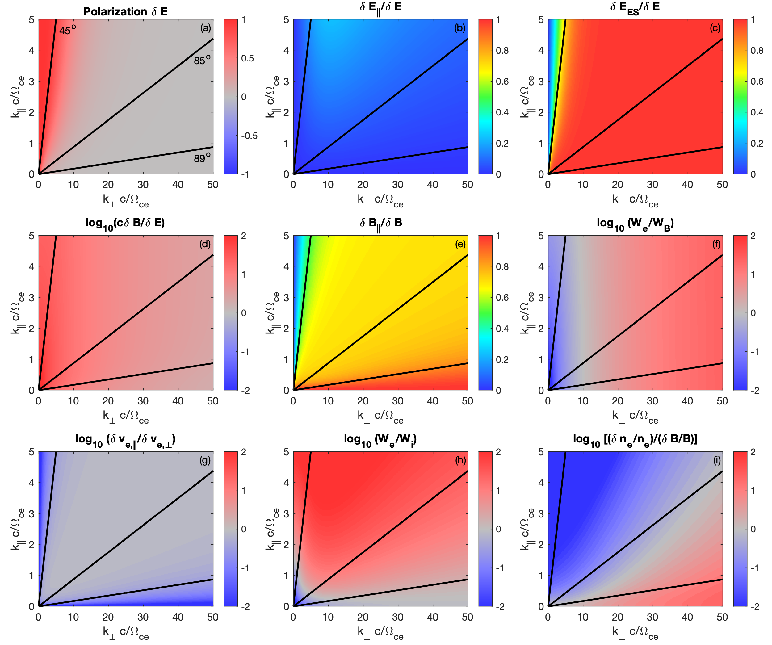
Figure 1: Properties of the whistler/lower hybrid dispersion surface as functions of $k_{\parallel}d_{e}$ and $k_{\perp}d_{e}$. The properties are calculated for $f_{pe}/f_{ce}=10$. (a) Ellipticity of the perpendicular electric field $\delta{\bf E}$. (b) Ratio of the parallel to total electric field $\delta{\bf E}_{\parallel}/\delta{\bf E}$. (c) Ratio of the electrostatic to total electric field $\delta{\bf E}_{ES}/\delta{\bf E}$. (d) $c\delta{\bf B}/\delta{\bf E}$. (e) Ratio of parallel to total magnetic field fluctuations $\delta{\bf B}_{\parallel}/\delta{\bf B}$. (f) Ratio of the electron energy density to magnetic field energy density $W_{e}/W_{B}$. (g) Ratio of parallel to perpendicular electron velocities $\delta{\bf V}_{e,\parallel}/\delta{\bf V}_{e,\perp}$. (h) Ratio of electron to ion energy densities $W_{e}/W_{i}$. (i) Ratio of density and magnetic field perturbations normalized to their background values $(\delta n_{e}/n_{e})/(\delta B/B)$.

We now summarize the properties of lower hybrid waves shown in Figure 1 and their relevance to MMS observations are Earth’s magnetopause.

(1) In Figure 1a we plot the ellipticity of the wave electric field $\delta{\bf E}$ with respect to the background magnetic field ${\bf B}$, where $+1$ indicates right-hand circular polarization, $-1$ indicates left-hand circular polarization, and $0$ indicates linear polarization. For $\theta_{kB}<45^{\circ}$, where the waves are whistler-like we observe clear right-hand polarization. Whereas for $\theta_{kB}>45^{\circ}$, we observe linear polarization. Therefore, in the homogeneous approximation considered here, linear polarization is expected for lower hybrid waves. The ellipticity of the wave magnetic field $\delta{\bf B}$ (not shown) is similar to $\delta{\bf E}$.

(2) In Figure 1b we plot the ratio of the parallel to total electric field $\delta{\bf E}_{\parallel}/\delta{\bf E}$. For the range of ${\bf k}$ expected for lower hybrid waves $\delta{\bf E}_{\parallel}$ is negligible. Such a small parallel component is extremely difficult to measure accurately at lower hybrid wave frequencies with MMS (often below the uncertainty level for MMS).

(3) In Figure 1c we plot the ratio of the electrostatic to total electric field $\delta{\bf E}_{ES}/\delta{\bf E}$, where $\delta{\bf E}_{ES}$ is the electric field aligned with ${\bf k}$. For $\theta_{kB}>45^{\circ}$, $\delta{\bf E}_{ES}/\delta{\bf E}\approx 1$ meaning the waves are approximately electrostatic and the electromagnetic $\delta{\bf E}$ is negligible. When the wave is whistler-like $\delta{\bf E}$ is primarily electromagnetic.

(4) In Figure 1d we plot the ratio $c\delta{\bf B}/\delta{\bf E}$, which indicates how large the magnetic field energy density $W_{B}=|\delta{\bf B}|^{2}/(2\mu_{0})$ is compared with the electric field energy density $W_{E}=\epsilon_{0}|\delta{\bf E}|^{2}/2$. For $f_{pe}/f_{ce}=10$, $c\delta{\bf B}/\delta{\bf E}>1$ for the range of ${\bf k}$ shown in Figure 1. We find that $c\delta{\bf B}/\delta{\bf E}$ decreases as $k_{\perp}$ increases. The fact that $c\delta{\bf B}/\delta{\bf E}$ scales with $k_{\perp}$ provides a way to estimate $k_{\perp}$ from $\delta{\bf B}$ and $\delta{\bf E}$ observations (see Appendix A). For $f_{pe}/f_{ce}=10$ there is more energy density in the magnetic field than in the electric field of the lower hybrid waves, despite $\delta{\bf E}\approx\delta{\bf E}_{ES}$. We thus refer to these waves as quasi-electrostatic. For constant $k_{\perp}d_{e}$, $c\delta{\bf B}/\delta{\bf E}$ increases as $f_{pe}/f_{ce}$ increases. For typical magnetopause conditions and lower hybrid wavelengths the ratio $W_{B}/W_{E}$ is often greater than one.

(5) In Figure 1e we plot the ratio $\delta{\bf B}_{\parallel}/\delta{\bf B}$, where $\delta{\bf B}_{\parallel}$ is the fluctuating magnetic field parallel to the background ${\bf B}$. For $k_{\perp}\gg k_{\parallel}$, $\delta{\bf B}_{\parallel}$ is the largest component of the fluctuating magnetic field, and for $k_{\parallel}\approx 0$, $\delta{\bf B}_{\parallel}\approx\delta{\bf B}$. The perpendicular $\delta{\bf B}_{\perp}$ becomes dominant for $k_{\parallel}>k_{\perp}$, when the wave is whistler-like. For lower hybrid waves observed at the subsolar magnetopause, which propagate in dawn-dusk direction, a finite $k_{\parallel}$ is expected to produce $\delta{\bf B}_{\perp}$ in the direction normal to the magnetopause because $\delta{\bf B}\cdot{\bf k}=0$ and ${\bf k}$ is tangential to the magnetopause.

(6) In Figure 1f we plot the ratio of electron energy density to magnetic field energy density $W_{e}/W_{B}$, where $W_{e}=n_{e}m_{e}|\delta{\bf V}_{e}|^{2}/2$ is the electron energy density. For the wave number range shown in Figure 1, $W_{e}/W_{B}$ depends strongly on $k_{\perp}$, with $W_{B}\gg W_{e}$ for low $k_{\perp}$ and $W_{e}\gg W_{B}$ for large $k_{\perp}$. Thus, $W_{e}/W_{B}$ provides a clear indicator of $k_{\perp}$. We find that $W_{e}=W_{B}$ for $k_{\perp}d_{e}=1$ when $k_{\perp}\gg k_{\parallel}$.

(7) In Figure 1g we plot the ratio of parallel to perpendicular electron fluctuations $\delta{\bf V}_{e,\parallel}/\delta{\bf V}_{e,\perp}$. For parallel and perpendicular ${\bf k}$ the electron fluctuations are perpendicular to ${\bf B}$. For oblique $\theta_{kB}$ between $45^{\circ}$ and $89^{\circ}$ the parallel and perpendicular fluctuations have comparable magnitudes. For $k_{\perp}\gg k_{\parallel}$, $\delta{\bf V}_{e,\parallel}/\delta{\bf V}_{e,\perp}$ depends strongly on $\theta_{kB}$, which provides a way to estimate $\theta_{kB}$ when $\delta{\bf V}$ is resolved.

(8) In Figure 1h we plot the ratio of $W_{e}$ to $W_{i}$, where $W_{i}=n_{i}m_{i}|\delta{\bf V}_{i}|^{2}/2$ is the ion energy density. For $\theta_{kB}\gtrsim 89^{\circ}$, $W_{e}$ and $W_{i}$ are approximately equal, meaning that $|\delta{\bf V}_{e}|\gg|\delta{\bf V}_{i}|$ due to the much lower mass of electrons. For $\theta_{kB}\lesssim 89^{\circ}$, we find that $W_{e}>W_{i}$, except at very small $k$. In general, $\delta{\bf V}_{i}$ at lower hybrid timescales is often under-resolved by MMS, so it is difficult to compare $W_{i}$ with $W_{e}$. However, since $m_{i}\gg m_{e}$, $\delta{\bf V}_{i}$ is expected to be small for lower hybrid waves, except for very low $k$.

(9) In Figure 1i we plot the ratio of normalized density perturbations to normalized magnetic field perturbations, $(\delta n_{e}/n_{e})/(|\delta{\bf B}|/|{\bf B}|)$. For lower hybrid-like waves $\delta n_{e}/n_{e}>|\delta{\bf B}|/|{\bf B}|$, with $(\delta n_{e}/n_{e})/(|\delta{\bf B}|/|{\bf B}|)$ increasing with $k$. The ratio $(\delta n_{e}/n_{e})/(|\delta{\bf B}|/|{\bf B}|)$ also increases as $f_{pe}/f_{ce}$ decreases. For whistler-like waves $\delta n_{e}/n_{e}<|\delta{\bf B}|/|{\bf B}|$. In other words, $(\delta n_{e}/n_{e})/(|\delta{\bf B}|/|{\bf B}|)$ increases as $\theta_{kB}$ increases. For $k_{\perp}\gg k_{\parallel}$, $(\delta n_{e}/n_{e})/(|\delta{\bf B}|/|{\bf B}|)$ depends strongly on $\theta_{kB}$, enabling $\theta_{kB}$ to be estimated from observations when $\delta n_{e}$ is resolved. We note that $\delta n_{e}/n_{e}$ potentially depends strongly on gradients in $B$ and $n_{e}$, so $(\delta n_{e}/n_{e})/(|\delta{\bf B}|/|{\bf B}|)$ may differ significantly from the homogeneous case when the waves occur at strong gradients (see Appendix A).

From the properties shown in Figure 1 we can compute important parameters of lower hybrid waves, including the wave number, dispersion relation, and wave-normal angle from single-spacecraft observations. In particular, we show that $W_{e}/W_{B}$ can be used to determine $k_{\perp}$. For lower hybrid waves the electrons are approximately frozen in, i.e., $\delta{\bf E}=-\delta{\bf V}_{e}\times{\bf B}$ (shown below). By assuming electrons are frozen in we can calculate $W_{e}$ and $W_{B}$ as a function of the electrostatic potential $\delta\phi$ (see Appendix A for details):

$$W_{e}=\frac{1}{2}n_{e}m_{e}\delta V_{e}^{2}=\frac{1}{2}\frac{n_{e}m_{e}}{B_{0}^{2}}\left(1+\frac{\omega_{ce}^{2}}{\omega^{2}}\frac{k_{\parallel}^{2}}{k_{\perp}^{2}}\right)k_{\perp}^{2}\delta\phi^{2},$$ (1)

$$W_{B}=\frac{1}{2}\frac{\delta B^{2}}{\mu_{0}}=\frac{1}{2}\left(1+\frac{\omega_{ce}^{2}}{\omega^{2}}\frac{k_{\parallel}^{2}}{k_{\perp}^{2}}\right)\frac{\delta\phi^{2}\mu_{0}e^{2}n_{e}^{2}}{B_{0}^{2}}.$$ (2)

By taking the ratio of $W_{e}$ and $W_{B}$ we can estimate the dispersion relation in the spacecraft reference frame using

$$\frac{W_{e}(\omega)}{W_{B}(\omega)}=d_{e}^{2}k_{\perp}^{2}(\omega)\rightarrow k_{\perp}(\omega)=\frac{1}{d_{e}}\sqrt{\frac{W_{e}(\omega)}{W_{B}(\omega)}},$$ (3)

where $W_{e}(\omega)$ and $W_{B}(\omega)$ are computed in the frequency domain using Fourier or wavelet methods. Thus, $k_{\perp}$ can be computed as a function of frequency (i.e., the dispersion relation) if the electron fluctuations are resolved. Similarly, we can estimate $k_{\parallel}$ and $\theta_{kB}$ when $k_{\perp}$ is known using $|\delta{\bf B}_{\parallel}|/|\delta{\bf B}|$, $(\delta n_{e}/n_{e})/(|\delta{\bf B}|/|{\bf B}|)$, and/or $\delta|{\bf V}_{e,\parallel}|/|\delta{\bf V}_{e,\perp}|$ as proxies. Using these parameters we can provide a reasonable estimate of $\theta_{kB}$ for lower hybrid waves, and potentially investigate whether they can interact with electrons to produce parallel electron heating.

3 MMS Data

We use data from the MMS spacecraft; we use electric field ${\bf E}$ data from electric field double probes (EDP) Lindqvist et al. (2016); Ergun et al. (2016), magnetic field ${\bf B}$ data from fluxgate magnetometer (FGM) Russell et al. (2016) and search-coil magnetometer (SCM) Le Contel et al. (2016), and particle data from fast plasma investigation (FPI) Pollock et al. (2016). All data presented in this paper are high-resolution burst mode data. To study lower hybrid waves we use the highest resolution electron moments, which are sampled at $133$ Hz Rager et al. (2018), which is typically sufficient to resolve fluctuations associated with lower hybrid waves at Earth’s magnetopause. The ion distributions and moments are sampled at $27$ Hz, which is typically not sufficient to fully resolve lower hybrid waves. These high time resolution electron distributions and moments are computed with reduced azimuthal coverage in the spacecraft spin plane, with the azimuthal coverage being reduced from 11.25^∘ to 45^∘ Pollock et al. (2016); Rager et al. (2018). However, since we are interested in the changes in the bulk distribution, rather than fine structures in the particle distribution functions, this reduced angular resolution does not present a major problem to the data analysis here.

To investigate the properties of lower hybrid waves, and the instabilities generating them, we study two events in detail: A broad magnetopause crossing observed on 28 November 2016 far from any reconnection diffusion region and a magnetopause crossing near the electron diffusion region observed on 14 December 2015. In both events the spacecraft were in a tetrahedral configuration.

4 28 November 2016

4.1 Event overview

We first investigate a magnetopause crossing on 28 November 2016 between 07:29:30 UT and 07:32:00 UT. The spacecraft were located at [10.0, 3.0, -0.3] in Geocentric Solar Ecliptic coordinates (GSE), close to the subsolar point. We transform the vector quantities into LMN coordinates based on minimum variance analysis of the magnetic field ${\bf B}$, where ${\bf L}=[0.26,0.09,0.96]$, ${\bf M}=[0.33,-0.94,-0.01]$, and ${\bf N}=[0.91,0.32,-0.28]$ in GSE coordinates. Based on timing analysis of $B_{L}$ we estimate that the magnetopause boundary moves at $\sim 40\,\mathrm{km}\,\mathrm{s}^{-1}$ in the $-{\bf N}$ direction (Earthward). The mean spacecraft separation was $\sim 6\,\mathrm{km}$. Figures 2a–2f provide an overview of the magnetopause crossing from the magnetosphere to the magnetosheath, identified by the increase in electron density $n_{e}$ (Figure 2c) and decrease in magnetic field strength (Figure 2a). Figure 2a shows that the magnetic field ${\bf B}$ remains northward ($B_{L}>0$) across the boundary until 07:31:15 UT when $B_{L}<0$ is observed. Across the density gradient we observe an enhancement in the ion bulk velocity ${\bf V}_{i}$ in the $-{\bf M}$ direction (Figure 2b). This is due to the finite gyroradius effect of magnetosheath ions entering the magnetosphere. Although this is a feature of magnetopause crossings close to the ion diffusion region, we see no clear evidence of a nearby diffusion region, such as the Hall electric field and electron jets. We observe a southward ion flow $V_{L}<0$ where $B_{L}$ changes sign, suggestive of an ion outflow. The yellow-shaded region in Figures 2a–2c indicates when the lower hybrid waves are observed. This region coincides with the density gradient and enhanced $V_{M}<0$ ion flow. In this case the density gradient is relatively weak and the waves are observed over an extended period of time.

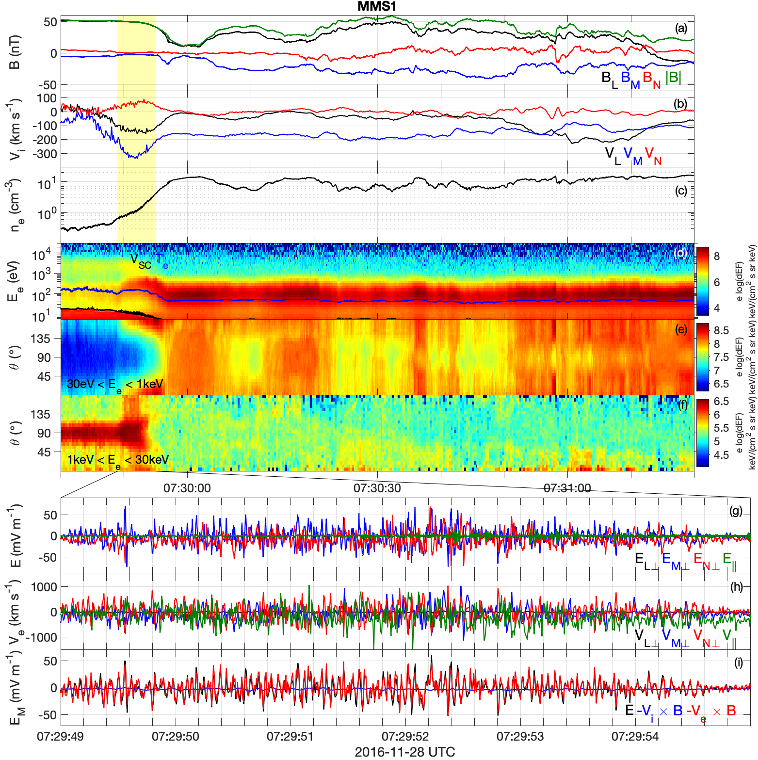
Figure 2: Overview of the magnetopause crossing observed on 28 November 2016 observed by MMS1. (a) ${\bf B}$. (b) ${\bf V}_{i}$. (c) $n_{e}$. (d) Electron omni-directional differential energy flux. (e) and (f) Electron pitch-angle distribution for electron energies $30\,\mathrm{eV}<E<1\,\mathrm{keV}$ and $1\,\mathrm{keV}<E<30\,\mathrm{keV}$, respectively. The yellow-shaded region indicates the region of intense lower hybrid wave activity. Panels (g)–(i) Overview of the lower hybrid waves observed in the yellow shaded region. (g) Perpendicular and parallel components of ${\bf E}$. (h) Perpendicular and parallel components of ${\bf V}_{e}$. (i) ${\bf M}$ components of ${\bf E}$ (black), the ion convection term $-{\bf V}_{i}\times{\bf B}$ (blue), and the electron convection term $-{\bf V}_{e}\times{\bf B}$ (red). In panels (b)–(f) we use the standard burst particle data and in panels (h) and (i) we use the highest resolution FPI data.

Figure 2d shows the electron omnidirectional energy flux. In the magnetosphere and near the magnetopause we observed both hot and colder electron populations. When the lower hybrid waves are observed there is an increase in energy of the colder electrons above the background level in the magnetosphere and in the magnetosheath. This corresponds to parallel electron heating, which can be seen as the large enhancement of electron fluxes parallel and antiparallel to ${\bf B}$ for electrons with energies $E<1\,\mathrm{keV}$ (Figure 2e). We find that $T_{\parallel}/T_{\perp}$ has a maximum of $4$ at 07:29:54.5 UT, which is comparable to some of the largest values found in the magnetospheric inflow regions of magnetopause reconnection Graham et al. (2016a, 2017a); Khotyaintsev et al. (2016); Wang et al. (2017). At high energies $E>1\,\mathrm{keV}$ the electrons have a strong perpendicular temperature anisotropy $T_{\parallel}/T_{\perp}<1$ in the magnetosphere and as the magnetopause boundary is approached (Figure 2f). At the beginning of the yellow-shaded region between 07:29:49 UT and 07:29:53 UT there is an enhancement in the flux of high-energy electrons. These high-energy electrons tend to broaden in pitch angle, although the perpendicular temperature anisotropy remains.

4.2 Lower hybrid wave observations

Figures 2g–2i provide an overview of the lower hybrid waves in the yellow-shaded region of Figures 2a–2c. Figure 2g shows the perpendicular and parallel components of ${\bf E}$. The lower hybrid waves are characterized by large-amplitude fluctuations in $E_{M\perp}$ and $E_{N\perp}$, reaching a peak amplitude of about $70$ mV m^-1. The fact that both $E_{M\perp}$ and $E_{N\perp}$ are observed and have different traces suggests that the waves are non-planar, and that complex structures, such as vortices, may be developing ($E_{L\perp}$ is close to field-aligned and therefore very small).

For this event the electron velocity fluctuations $\delta{\bf V}_{e}$ are resolved by FPI using the highest cadence moments. Figure 2h shows the perpendicular and parallel components of the electron velocity ${\bf V}_{e}$. Large-amplitude fluctuations in $V_{N\perp}$, $V_{M\perp}$, and $V_{\parallel}$ are observed, which each reach amplitudes of $\approx 1000$ km s^-1. The fact that large $\delta V_{\parallel}$ are observed indicates that the waves have a finite $k_{\parallel}$ (cf., Figure 1g). In Figure 2i we plot $E_{M}$ versus the ${\bf M}$ components of ion and electron convection terms, $-{\bf V}_{i}\times{\bf B}$ and $-{\bf V}_{e}\times{\bf B}$, respectively. For direct comparison we have downsampled the electric field to the same cadence as the electron moments. Throughout the interval ${\bf E}_{\perp}\approx-{\bf V}_{e}\times{\bf B}$, as expected for lower hybrid waves. This result also confirms that the high-resolution ${\bf V}_{e}$ is reliable. Overall, $-{\bf V}_{i}\times{\bf B}$ remains small, as expected for lower hybrid waves. However, we note that the resolution of the ion moments is not sufficient to fully resolve the lower hybrid waves here. We also observe large density perturbations associated with the waves (not shown), which reach a peak amplitude of $\delta n_{e}/n_{e}\approx 0.2$.

The fluctuating $\delta{\bf E}$ and $\delta{\bf B}$ of the lower hybrid waves and the associated wavelet spectrograms are shown in Figure 3. The fluctuations are broadband with power peaking just below the local lower hybrid frequency $f_{LH}$ (Figure 3e). The associated magnetic field fluctuations (Figures 3f and 3g) are primarily parallel to ${\bf B}$. These parallel magnetic field fluctuations $\delta B_{\parallel}$ peak at the same frequency as the perpendicular electric field fluctuations $\delta{\bf E}_{\perp}$. The combined $\delta{\bf E}_{\perp}$ and $\delta B_{\parallel}$ are consistent with previous observations of lower hybrid waves Norgren et al. (2012); Khotyaintsev et al. (2016); Graham et al. (2016a, 2017a), and suggest propagation approximately perpendicular to ${\bf B}$. The lower hybrid waves are observed for $\approx 6\,\mathrm{s}$ on each spacecraft, so the waves occur over a width of $\sim 240\,\mathrm{km}$ in the direction normal to the magnetopause, based on the estimated magnetopause velocity of $40$ km s^-1, suggesting that the local gradients are weak.

To investigate the electron heating associated with the thermal electron population we calculate $T_{\parallel}$ and $T_{\perp}$ for thermal electrons with energies $E<1\,\mathrm{keV}$ (Figure 3c). The thermal electrons in the magnetosphere have a slight parallel temperature anisotropy. By comparing Figure 3c with Figure 3d we see that the lower hybrid waves and parallel electron heating both start to develop at 07:29:49.0 UT, but lower hybrid activity is reduced when $T_{\parallel}/T_{\perp}$ peaks at 07:29:54.5 UT, similar to previous observations of asymmetric reconnection Graham et al. (2016a, 2017a). Figure 3c also shows the predicted $T_{\parallel}$ and $T_{\perp}$ from the equations of state (EoS) of the electron trapping model in Le et al. (2009) and Egedal et al. (2013), based on the upstream magnetospheric plasma conditions. We find good agreement between the predicted and observed $T_{\parallel}$ and $T_{\perp}$ between 07:29:50.0 UT and $\sim$07:29:52.0 UT, consistent with trapping of magnetospheric electrons. After this the EoS prediction, as well as the Chew-Goldberger-Low (CGL) scalings Chew et al. (1956) (not shown), overestimate $T_{\parallel}$. This is likely due to the mixing of magnetospheric and magnetosheath electrons. We also see that $T_{\perp}$ is slightly larger than the predicted value after 07:29:52.0 UT, which could be due to perpendicular electron heating by the lower hybrid waves Daughton (2003). Overall, the deviation in the observed $T_{\parallel}$ and $T_{\perp}$ from the predicted values suggests that the lower hybrid waves scatter electrons and enable magnetosheath electrons to enter the magnetosphere, possibly by cross-field diffusion Graham et al. (2017a).

Figure 3: Overview of the electric and magnetic fields at the 28 November 2016 magnetopause crossing. (a) ${\bf B}$. (b) $n_{e}$. (c) Electron $T_{\parallel}$ and $T_{\perp}$ (black and red lines). The blue and green lines are $T_{\parallel}$ and $T_{\perp}$ predicted from EoS. (d) Perpendicular and parallel components of the fluctuating ($f>3\,\mathrm{Hz}$) electric field $\delta{\bf E}$. (e) Spectrogram of ${\bf E}$. (f) Perpendicular and parallel components of the fluctuating ($f>3\,\mathrm{Hz}$) magnetic field $\delta{\bf B}$. (g) Spectrogram of ${\bf B}$. In (e) and (g) the black and red curves are $f_{LH}$ and $f_{ce}$, respectively. (h) High-frequency $\delta E_{\parallel}$ and (i) the associated spectrogram (the white line is $f_{pe}$).

We also observe smaller-amplitude higher-frequency parallel electric fields $\delta E_{\parallel}$ in the same region as the lower hybrid waves and large $T_{\parallel}/T_{\perp}$. Figures 3h and 3i show $\delta E_{\parallel}$ and the associated spectrogram. The spectrogram shows that the waves have frequencies ranging from a few hundred Hz to the local electron plasma frequency $f_{pe}$. These $\delta E_{\parallel}$ are associated with bipolar electrostatic solitary waves (ESWs), and more periodic electrostatic waves. We observe ESWs with distinct time-scales suggesting that both fast and slow ESWs occur in this region Graham et al. (2015). The electrostatic waves develop between 07:29:51.5 UT and 07:29:56 UT as seen in Figures 3d and 3e, meaning these waves occur in the region with largest $T_{\parallel}/T_{\perp}$ rather than span the entirety of the region of lower hybrid waves. Before 07:29:51.5 UT large-amplitude lower hybrid waves are observed but there are negligible high-frequency $E_{\parallel}$ fluctuations, thus the $\delta E_{\parallel}$ waves are more closely correlated to large $T_{\parallel}/T_{\perp}$ than with the lower hybrid waves. The region where the higher-frequency waves occur roughly coincides with when the observed $T_{\parallel}/T_{\perp}$ deviates significantly from the EoS prediction, which suggests that the electrostatic waves are associated with mixing of magnetospheric and magnetosheath electrons. The electrostatic waves roughly occur over the region where $T_{\parallel}/T_{\perp}>2$, and may be generated by parallel electron streaming instabilities, rather than by the lower hybrid waves Che et al. (2010).

4.3 Lower Hybrid Wave Properties

In this subsection we investigate the field and particle properties of the lower hybrid waves and compare them with the predictions in Figure 1. In Figure 4 we compute the wavelet spectrograms of the energy densities of the fields and electrons observed by MMS1. To directly compare ${\bf B}$ and ${\bf E}$ with the electrons we have down-sampled ${\bf B}$ and ${\bf E}$ to same cadence as the high-resolution electron data. Figure 4a shows the perpendicular and parallel components of ${\bf E}$ (without down-sampling), associated with the lower hybrid waves. In Figure 4b we plot the spectrogram of $cB/E$. Throughout the interval $cB/E\gtrsim 1$ for the lower hybrid waves. We find that $cB/E$ tends to decrease as the frequency increases, consistent with $k_{\perp}$ increasing with frequency (cf., Figure 1d). We also find that $cB/E$ increases as $n_{e}$ increases and $B$ decreases, as expected when the plasma becomes more weakly magnetized ($f_{pe}/f_{ce}$ increases).

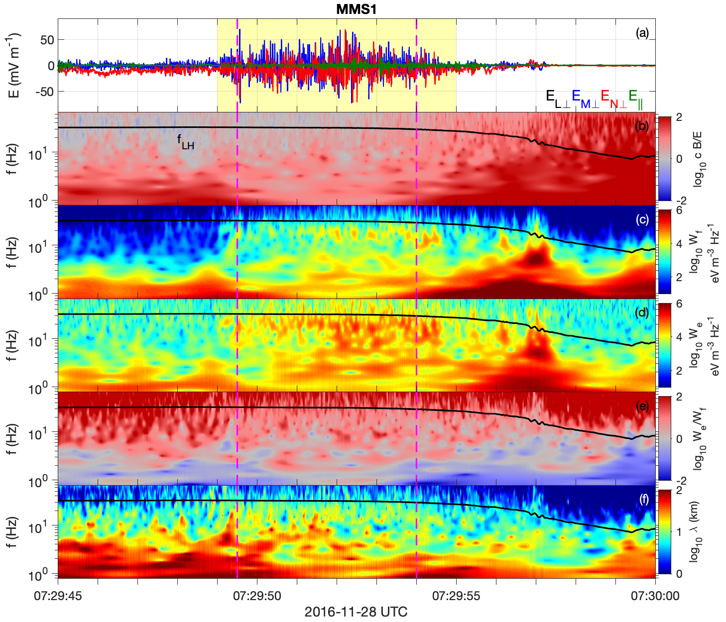
Figure 4: Properties of the lower hybrid waves observed on 28 November 2016 by MMS1. (a) ${\bf E}$ in field-aligned coordinates. (b) Spectrogram of $cB/E$. (c) Spectrogram of $W_{f}$. (d ) Spectrogram of electron energy density $W_{e}$. (e) Spectrogram of $W_{e}/W_{f}$. (f) Spectrogram of $\lambda$. The black lines in panels (b)–(f) indicate the local $f_{LH}$. The magenta vertical dashed lines mark the bound the interval over which we compute the average dispersion relation and $\theta_{kB}$.

In Figures 4c and 4d we plot spectrograms of the total field energy density $W_{f}=W_{E}+W_{B}$ and $W_{e}$. Large enhancements in $W_{f}$ and $W_{e}$ are observed at frequencies $f\sim 10-30$ Hz, just below the local $f_{LH}$, associated with the waves. We also observe a large enhancement in $W_{f}$ (due to ${\bf B}$ fluctuations) and $W_{e}$ at 07:29:57.0 UT. In Figure 4e we plot the spectrogram $W_{e}/W_{f}$, which shows that most of the energy density is in the electrons rather than the fields for these lower hybrid waves. In addition, $W_{e}/W_{f}\approx W_{e}/W_{B}$ tends to increase with $f$, consistent with increasing $k_{\perp}$ (cf., Figure 1f).

A spectrogram of the wavelength $\lambda$ can be calculated from $W_{e}$ and $W_{B}$. The spectrogram of $\lambda$ is computed using

$$\lambda(\omega)=2\pi d_{e}\sqrt{\frac{W_{B}(\omega)}{W_{e}(\omega)}}$$ (4)

from rearranging equation (3). In Figure 4f we show the spectrogram of wavelengths $\lambda$ (essentially the dispersion relation associated with the waves). We find that $\lambda$ tends to decrease with increasing frequency. For the lower hybrid waves we estimate $\lambda\sim 10-20$ km in the 10-30 Hz frequency range, where $W_{e}$ peaks.

We now use these spectrograms of $W_{e}$ and $W_{B}$ to construct the dispersion relation of the waves for each spacecraft. To obtain a single dispersion relation we take the median over time of $W_{e}/W_{B}$ for each frequency to compute $k_{\perp}$. We take this median over the time interval bounded by the magenta lines in Figure 4. The dispersion relations from each spacecraft are shown in Figure 5a. The color of the points indicates $W_{E}/W_{E,max}$, where $W_{E,max}$ is the maximum median value of $W_{E}$. As expected $\omega/\omega_{LH}$ increases with $k_{\perp}\rho_{e}$, where $\rho_{e}$ is the median electron thermal gyroradius. The characteristic frequencies and wave numbers of the lower hybrid waves are indicated by the largest $W_{E}/W_{E,max}$. We find that the observed waves have $0.3\lesssim k_{\perp}\rho_{e}\lesssim 0.5$ and frequencies $0.5\lesssim\omega/\omega_{LH}\lesssim 0.8$. This corresponds to $9\,\mathrm{km}\lesssim\lambda\lesssim 15\,\mathrm{km}$. All spacecraft observe very similar dispersion relations, which is not surprising since the spacecraft are separated by $\sim 6$ km, smaller than the estimated $\lambda$ of the waves. In Figure 5b we plot the phase speed $v_{ph}=\omega/k_{\perp}$ versus $k_{\perp}\rho_{e}$. In the range where the electric field power is concentrated, $W_{E}\gtrsim 0.6W_{E,max}$, we find that $200$ km s${}^{-1}\lesssim v_{ph}\lesssim 240$ km s^-1. Overall, the computed wave properties all agree with expectations for quasi-electrostatic lower hybrid waves.

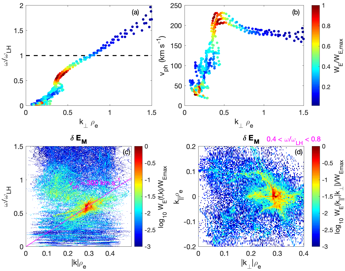
Figure 5: Dispersion relation of lower hybrid waves calculated using equation (3) [panels (a) and (b)] and dispersion relation computed from the phase differences of $\delta E_{M}$ between the spacecraft [(c) and (d)]. (a) Dispersion relations of the lower hybrid waves observed between the magenta dashed lines in Figure 4. The black dashed lined indicates $\omega/\omega_{LH}=1$. (b) Phase speed $v_{ph}$ versus $k_{\perp}\rho_{e}$. In both panels the color of the points indicates the value of $W_{E}/W_{E,max}$ of each frequency. (c) $W_{E}/W_{E,max}$ versus $\omega/\omega_{LH}$ and $k\rho_{e}$. (d) $W_{E}/W_{E,max}$ versus $k_{\parallel}\rho_{e}$ and $|k_{\perp}|\rho_{e}$ in the frequency range $0.3<\omega/\omega_{LH}<0.8$.

These calculations suggest that $\lambda$ is larger than the spacecraft separations, so we can compute the frequency/wave number power spectrum using the phase differences between the spacecraft to determine the wave vector ${\bf k}$. Figures 5c and 5d show the power spectra of $\delta E_{M}$ over the same time interval as Figures 5a and 5b, using the phase differences between the different spacecraft pairs to determine ${\bf k}$. We use the same method as Graham et al. (2016b), but generalized to four points. Figure 5c shows $W_{E}$ versus $\omega/\omega_{LH}$ and $k_{\perp}\rho_{e}$. We find that $W_{E}$ peaks at $k_{\perp}\rho_{e}=0.29$, which is slightly smaller than the values predicted in Figure 5a, and corresponds to $\lambda=16\,\mathrm{km}$. For the peak $W_{E}$ we calculate $v_{ph}=300$ km s^-1, which is slightly larger than the values predicted in Figure 5b. Figure 5d shows $W_{E}$ versus $k_{\parallel}$ and $k_{\perp}$. We find the largest $W_{E}$ for $k_{\perp}\gg k_{\parallel}$, although power at finite $k_{\parallel}$ is observed, which is consistent with the observed $\delta V_{e,\parallel}$ in Figure 2h.

We now estimate $k_{\parallel}$ and the wave-normal angle $\theta_{kB}$ over the same interval used to compute the dispersion relation using the parameters $\delta B_{\parallel}/\delta B$, $\delta V_{e,\parallel}/V_{e,\perp}$, and $(\delta n_{e}/n_{e})/(\delta B/B)$. Figures 6a–6c show $\delta B_{\parallel}/\delta B$, $\delta V_{e,\parallel}/V_{e,\perp}$, and $(\delta n_{e}/n_{e})/(\delta B/B)$ versus $k_{\parallel}$ and $k_{\perp}$. For these figures we use $f_{pe}/f_{ce}=6.7$, corresponding to the median observed $f_{pe}/f_{ce}$ for this interval. From the observed dispersion relation we obtain $k_{\perp}d_{e}\approx 3$, indicated by the green lines in Figures 6a–6c. In Figures 6d–6f we plot $\delta B_{\parallel}/\delta B$, $\delta V_{e,\parallel}/V_{e,\perp}$, and $(\delta n_{e}/n_{e})/(\delta B/B)$ versus $k_{\parallel}d_{e}$ for $k_{\perp}d_{e}=3$. All parameters vary rapidly with $k_{\parallel}$ in the limit $k_{\parallel}\ll k_{\perp}$.

In Figures 6g–6i we plot the observed $\delta B_{\parallel}/\delta B$, $\delta V_{e,\parallel}/V_{e,\perp}$, and $(\delta n_{e}/n_{e})/(\delta B/B)$ versus $k_{\perp}d_{e}$ associated with the lower hybrid waves observed by each spacecraft. In Figure 6g we find that $\delta B_{\parallel}/\delta B\approx 0.9$, which corresponds to $k_{\parallel}d_{e}\approx 0.04$ in Figure 6d. Similarly, for $\delta V_{e,\parallel}/\delta V_{e,\perp}$ we obtain $\approx 0.4$, corresponding to $k_{\parallel}d_{e}\approx 0.06$. Thus, the two quantities yield consistent estimates of $k_{\parallel}$. For $(\delta n_{e}/n_{e})/(\delta B/B)$ we obtain $\sim 12$ from observations, which is slightly larger than the maximum prediction for $k_{\perp}d_{e}=3$. This is likely due to the low plasma density $n_{e}\approx 1$ cm^-3. For lower densities the signal to noise level can be large, due to lower counting statistics, causing $\delta n_{e}/n_{e}$ to be overestimated. Thus, higher $n_{e}$ should be more favorable for computing $\delta n_{e}/n_{e}$.

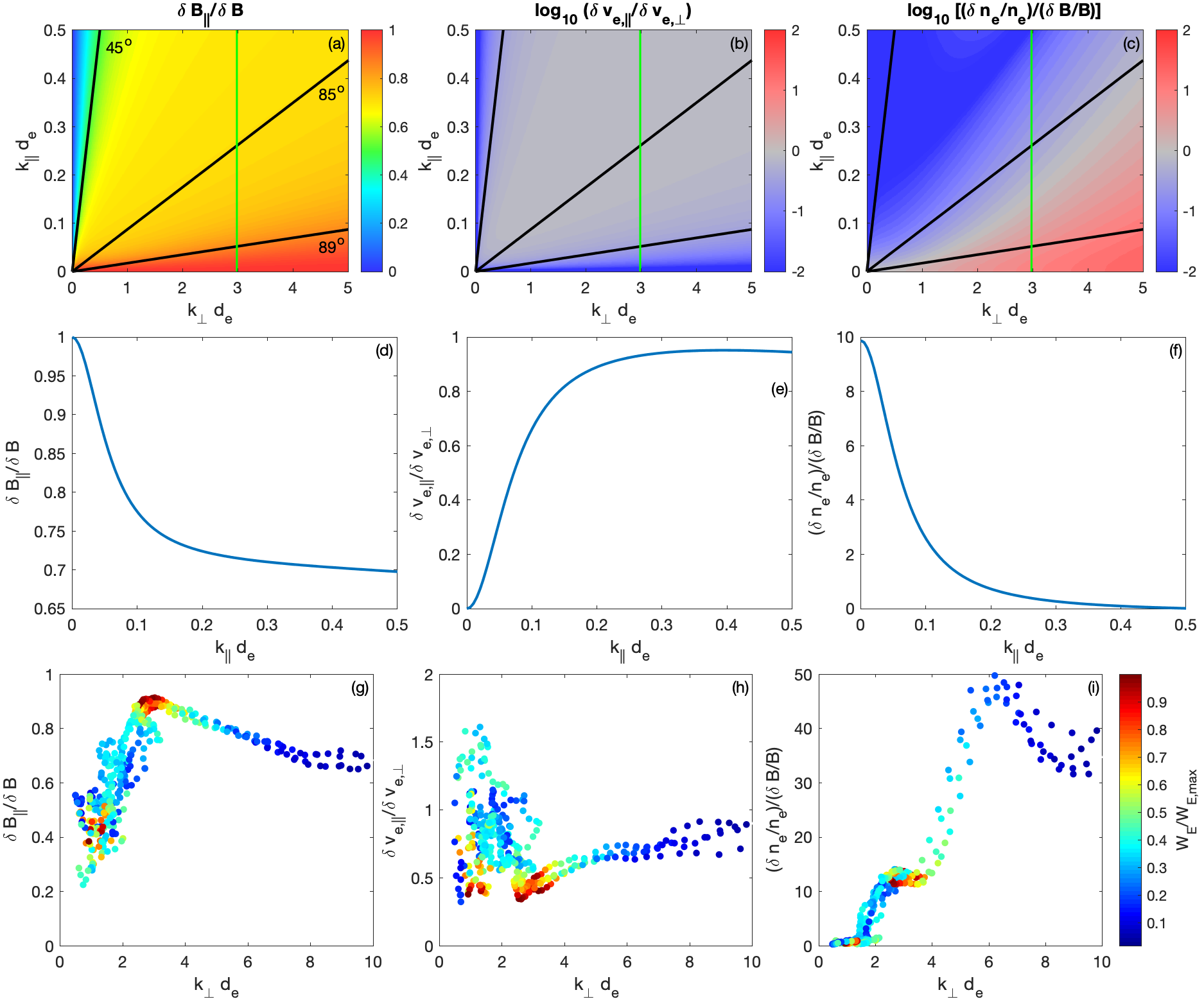
Figure 6: Estimates of the wave-normal angle and $k_{\parallel}$ from fields and particle observations of the lower hybrid waves observed on 28 November 2016. (a)–(c) $\delta B_{\parallel}/\delta B$, $\delta V_{e,\parallel}/V_{e,\perp}$, and $(\delta n_{e}/n_{e})/(\delta B/B)$ for whistler/lower hybrid waves versus $k_{\parallel}$ and $k_{\perp}$. We use $f_{pe}/f_{ce}=6.7$. The green line is $k_{\perp}d_{e}=3$, the estimate $k_{\perp}$ of the observed waves. (d)–(f) $\delta B_{\parallel}/\delta B$, $\delta V_{e,\parallel}/V_{e,\perp}$, and $(\delta n_{e}/n_{e})/(\delta B/B)$ versus $k_{\parallel}d_{e}$ for $k_{\perp}d_{e}=3$. (g)–(i) Observed $\delta B_{\parallel}/\delta B$, $\delta V_{e,\parallel}/V_{e,\perp}$, and $(\delta n_{e}/n_{e})/(\delta B/B)$ of the lower hybrid waves versus $k_{\perp}d_{e}$. The colors of the points indicate $W_{E}/W_{E,max}$.

Based on the observations in Figures 6g and 6h we estimate $k_{\parallel}d_{e}\approx 0.05$, corresponding to a wave-normal angle of $\theta_{kB}=\tan^{-1}(k_{\perp}/k_{\parallel})\approx 89^{\circ}$. This value is consistent with the four spacecraft observation in Figure 5d. Since $k_{\parallel}$ is known we can estimate the parallel resonance speed/energy $v_{\parallel}=\omega/k_{\parallel}$. From the estimates in Figures 5 and 6 we obtain $v_{\parallel}\sim 500$ eV. This energy is above the peak parallel electron thermal energy $T_{e,\parallel}\sim 250$ eV, which suggests that the waves can interact with suprathermal electrons. As $k_{\parallel}$ increases $v_{\parallel}$ decreases, which will result in stabilization by Landau damping. Overall, the estimated $\theta_{kB}$ is in excellent agreement with values predicted for quasi-electrostatic lower hybrid waves.

4.4 Single-Spacecraft and Multi-Spacecraft Observations of Lower Hybrid Waves

We now use the single-spacecraft method developed in Norgren et al. (2012) to calculate ${\bf v}_{ph}$ and compare with the results in section 4.3 and four-spacecraft timing analysis, as well as investigate how the wave properties change as the magnetopause is approached. The wave potential is related to the magnetic field fluctuations parallel to ${\bf B}$ by Norgren et al. (2012)

$$\delta\phi_{B}=\frac{|{\bf B}|\delta B_{\parallel}}{en_{e}\mu_{0}}.$$ (5)

The wave potential is also determined from the fluctuating electric field $\delta{\bf E}$, using

$$\delta\phi_{E}=\int\delta{\bf E}\cdot{\bf v}_{ph}dt.$$ (6)

The phase speed and direction are found by determining the best fit of $\delta\phi_{E}$ to $\delta\phi_{B}$. The wavelength and $k$ are found using $\lambda=v_{ph}/f$, where $f$ is the wave frequency. Using this method we have assumed the waves propagate perpendicular to ${\bf B}$, which is justified because the estimated $k_{\parallel}$ is small compared with $k_{\perp}$. Equation (5) assumes electrons are frozen-in, which is justified based on Figure 2i. We bandpass the fields above $10$ Hz. We also estimate ${\bf v}_{ph}$ using the time offsets between the four spacecraft.

As an example we compare the single-spacecraft method [equations (5) and (6)] with four-spacecraft timing for a short interval of lower hybrid wave activity, shown in Figure 7. Figures 7a–7d show $\delta\phi_{B}$ and $\delta\phi_{E}$ as well as the calculated ${\bf v}_{ph}$ for MMS1–4, respectively. For all spacecraft $\delta\phi_{B}$ and $\delta\phi_{E}$ show excellent agreement with correlation coefficients $C_{\phi}$ between $\delta\phi_{B}$ and $\delta\phi_{E}$ close to $1$. All spacecraft yield propagation directions close to the $-{\bf M}$ direction; the same direction as the cross-field ion flow. The phase speeds range from $v_{ph}=240\,\mathrm{km}\,\mathrm{s}^{-1}$ to $320\,\mathrm{km}\,\mathrm{s}^{-1}$, with a mean of $270\,\mathrm{km}\,\mathrm{s}^{-1}$. The approximate wave frequency is $f\approx 18\,\mathrm{Hz}$, whence we calculate $\lambda\approx 15\,\mathrm{km}$, in agreement with the estimates in section 4.3.

Figures 7e and 7f show $\delta E_{M}$ from the four spacecraft without time offsets and $\delta E_{M}$ with time offsets applied to find the best overlap of the waveforms over the interval. The velocity of the waves past the spacecraft is then determined from the time offsets. We calculate ${\bf v}_{ph}\approx 280\,\mathrm{km}\,\mathrm{s}^{-1}$ in the $-{\bf M}$ direction, in excellent agreement with the mean ${\bf v}_{ph}$ from the single-spacecraft method. The angle between ${\bf k}$ and ${\bf B}$ is $\theta_{kB}=87^{\circ}$, consistent with near perpendicular propagation. We apply the same timing analysis to $\delta B_{\parallel}$ in Figures 7g and 7h and find very good agreement with ${\bf v}_{ph}$ computed from $\delta E_{M}$ timing and the single-spacecraft estimates. Based on the $\delta B_{\parallel}$ timing we calculate ${\bf v}_{ph}\approx 300\,\mathrm{km}\,\mathrm{s}^{-1}$ and $\theta_{kB}=84^{\circ}$. Thus, $\delta E_{M}$ and $\delta B_{\parallel}$ propagate together at approximately the same velocity, as expected for lower hybrid waves. For both $\delta E_{M}$ and $\delta B_{\parallel}$ with time offsets applied the waveforms remain in phase and overlap well over multiple wave periods, which shows that the timing analyses are reliable. These results show that single-spacecraft methods used to calculate the lower hybrid waves can be reproduced using four-spacecraft methods, which confirms their reliability.

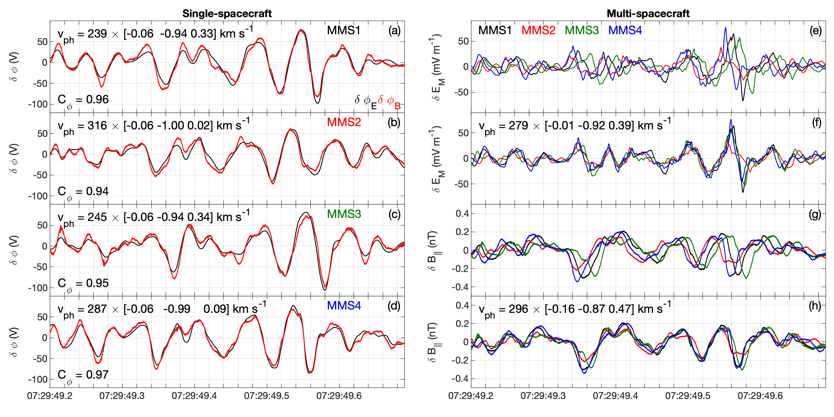
Figure 7: Part of the lower hybrid wave interval observed by the four spacecraft. (a)–(d) $\delta\phi_{E}$ and $\delta\phi_{B}$ observed by each spacecraft. The computed phase velocities (in LMN coordinates) and $C_{\phi}$ are stated in each panel. (e) $\delta E_{M}$ observed by the four spacecraft. (f) $\delta E_{M}$ with time offsets applied to estimate ${\bf v}_{ph}$. (g) $\delta B_{\parallel}$ observed by the four spacecraft. (h) $\delta B_{\parallel}$ with time offsets applied to estimate ${\bf v}_{ph}$. We bandpass filter above $10\,\mathrm{Hz}$ to obtain $\delta E_{M}$ and $\delta B_{\parallel}$.

We can investigate how the properties change across the boundary because the lower hybrid waves are observed over an extended period of time. Figure 8 shows the results based on the single-spacecraft method and four-spacecraft timing in the yellow-shaded region of Figures 2–4. For the single-spacecraft method we use 0.5 s intervals and perform the calculations for each spacecraft every 0.25 s. For the four-spacecraft timing of $\delta E_{M}$ and $\delta B_{\parallel}$ we calculate ${\bf v}_{ph}$ by estimating the time delays in the peaks in the waveforms. Figures 8a and 8b show $\delta E_{M}$ and $\delta\phi_{B}$ from the four spacecraft. The waveforms remain similar to each other across the boundary but tend to be more similar at earlier times, further from the boundary. We find that $\delta\phi_{B}$ remains very large throughout the interval with a peak of $\delta\phi_{\mathrm{max}}\approx 120\,\mathrm{V}$, corresponding to $e\delta\phi_{\mathrm{max}}/k_{B}T_{e}\approx 0.7$. Such large values of $\delta\phi_{B}$ suggest that the waves have amplitudes close to saturation.

Figure 8c shows that throughout the interval the correlation coefficient $C_{\phi}$ between $\phi_{E}$ and $\phi_{B}$ remains close to 1, indicating that the single-spacecraft method is very reliable. The phase speeds $v_{ph}$ calculated from the single-spacecraft method are shown in Figure 8d. Each spacecraft shows similar results, with $v_{ph}$ tending to decrease toward the boundary (the magenta line shows $v_{ph}$ averaged over the four spacecraft). The propagation direction is consistently in the $-{\bf M}$ direction in the spacecraft frame. However, throughout most of the interval $v_{ph}$ is less than ${\bf V}_{i}$ in the $-{\bf M}$ direction. Therefore, in the bulk ion frame the waves tend to propagate in the ${\bf M}$ direction. Figures 8g and 8h show the wavelength $\lambda$ and $k_{\perp}\rho_{e}$ computed from the averaged $v_{ph}$ and $f\approx 18\,\mathrm{Hz}$. The predicted $\lambda$ decreases toward the magnetopause as $v_{ph}$ decreases, while $k_{\perp}\rho_{e}$ remains relatively constant with $0.3\lesssim k_{\perp}\rho_{e}\lesssim 0.4$, which agrees with the observations in Figure 5. These values are slightly smaller than the typical $k_{\perp}\rho_{e}\approx 0.5-1$ observed at the magnetopause Graham et al. (2016a, 2017a); Khotyaintsev et al. (2016), but consistent with lower hybrid waves. Throughout the region $\lambda$ remains larger than the spacecraft separations, enabling timing analysis to be used although the uncertainty in the timing analysis increases with decreasing $\lambda$ because the differences in the waveforms between the spacecraft become more substantial.

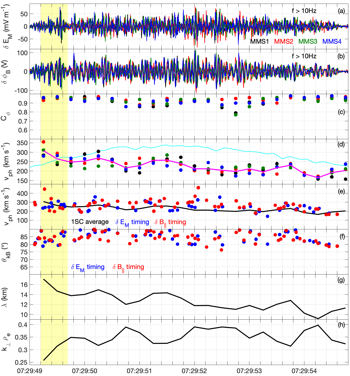
Figure 8: Lower hybrid wave properties calculated using the single-spacecraft method and multi-spacecraft timing over the yellow-shaded regions in Figures 2–4. (a) $\delta E_{M}$ observed by MMS1 (black), MMS2 (red), MMS3 (green), and MMS4 (blue). (b) $\delta\phi_{B}$ computed for MMS1–4. (c) $C_{\phi}$ for MMS1–MMS4 using the one-spacecraft method. (d) $v_{ph}$ for MMS1–MMS4 using the one-spacecraft method. The magenta curve is the average from the four spacecraft and the cyan curve is four-spacecraft averaged bulk ion speed in the ${\bf M}$ direction, $|V_{i,M}|$. (e) $v_{ph}$ from the four-spacecraft average of the single-spacecraft method (black), and from timing analysis of $\delta E_{M}$ (blue) and $\delta B_{\parallel}$ (red). (f) $\theta_{kB}$ from timing analysis of $\delta E_{M}$ (blue) and $\delta B_{\parallel}$ (red). (g) and (h) $\lambda$ and $k_{\perp}\rho_{e}$ computed from the four-spacecraft average of the single-spacecraft method using $f=18\,\mathrm{Hz}$. The yellow-shaded region is the time interval used in Figure 7.

Figures 8e and 8f show $v_{ph}$ and $\theta_{kB}$ based on timing analysis of $\delta E_{M}$ and $\delta B_{\parallel}$. Throughout the region $v_{ph}$ calculated from timing of $\delta E_{M}$ and $\delta B_{\parallel}$ agree well with each other and the single-spacecraft observations. Statistically, there is negligible difference between $v_{ph}$ and $\theta_{kB}$ calculated from $\delta E_{M}$ and $\delta B_{\parallel}$, confirming that both the $\delta E_{M}$ and $\delta B_{\parallel}$ perturbations propagate at the same ${\bf v}_{ph}$. The waves propagate approximately perpendicular to ${\bf B}$ (for all points the propagation direction was close to the $-{\bf M}$ direction). We find that $75^{\circ}\lesssim\theta_{kB}<90^{\circ}$, with an average of $\theta_{kB}\approx 85^{\circ}$. The spread in values of $\theta_{kB}$ likely provide an indicator of the uncertainty in the four-spacecraft timing, rather than the actual $\theta_{kB}$.

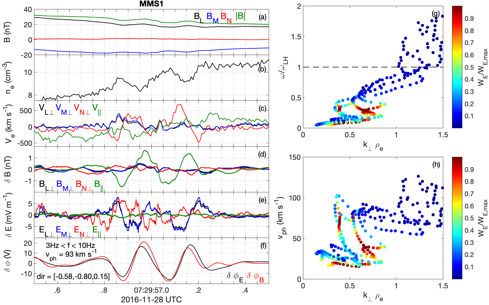
Figure 9: Lower hybrid waves observed close to the magnetopause boundary. (a) ${\bf B}$. (b) $n_{e}$. (c) Perpendicular and parallel components of ${\bf V}_{e}$. (d) Perpendicular and parallel components of $\delta{\bf B}$ ($f>2\,\mathrm{Hz}$). (e) Perpendicular and parallel components of $\delta{\bf E}$ ($f>2\,\mathrm{Hz}$). (f) $\delta\phi_{E}$ and $\delta\phi_{B}$. The results from the single-spacecraft analysis are stated in the panel. (g) Dispersion relation from all four spacecraft. (h) Phase speed $v_{ph}$ versus $k_{\perp}$ from all four spacecraft.

Figure 9 shows the waves characterized by large $\delta B_{\parallel}$ observed at 07:29:57 UT in Figure 3. The waves have frequency $f\approx 5\,\mathrm{Hz}$, so the fluctuations in $n_{e}$ and electron velocity ${\bf V}_{e}$ associated with the wave are well resolved by FPI. The waves are observed at relatively high ion plasma beta, $\beta_{i}\sim 4$, in contrast to the waves described above. Figures 9a and 9d show that $\delta B_{\parallel}$ is sufficiently large to significantly modify the total magnetic field $|{\bf B}|$. Figure 9d shows that there is negligible $\delta{\bf B}$ perpendicular to the background ${\bf B}$, so the amplitude of ${\bf B}$ is changed, rather than the direction. In addition, density fluctuations $\delta n_{e}$ are observed, which are anticorrelated with $\delta B_{\parallel}$. Similar fluctuations in the ion density $\delta n_{i}$ are observed (not shown), while the ion velocity fluctuations are negligible. This behavior is consistent with lower hybrid waves found in simulations Pritchett et al. (2012); Le et al. (2017). The fluctuations in ${\bf V}_{e}$ are primarily in the ${\bf N}$ direction, consistent with $\delta{\bf E}\times{\bf B}$ drifting electrons, due to the wave electric field (Figure 9e). The electric field associated with the waves is significantly smaller than the lower hybrid waves observed earlier. We apply the single-spacecraft method to the waves in Figure 9f, to determine the wave properties. We find good correlation between $\delta\phi_{B}$ and $\delta\phi_{E}$, with $C_{\phi}=0.92$. Despite the small amplitude of $\delta{\bf E}$ the waves have a peak potential of $\delta\phi_{\mathrm{max}}\approx 20\,\mathrm{V}$, corresponding to $e\delta\phi_{\mathrm{max}}/k_{B}T_{e}\approx 0.4$. We estimate a phase speed of $v_{ph}\approx 90\,\mathrm{km}\,\mathrm{s}^{-1}$ close to the $-{\bf M}$ direction, whence we calculate $\lambda\approx 19\,\mathrm{km}$ for $f\approx 5\,\mathrm{Hz}$. Despite this large $\lambda$ we are not able to perform four-spacecraft timing analysis, which might suggest that the waves are highly localized in the ${\bf N}$ direction. This $\lambda$ corresponds to $k_{\perp}\rho_{e}\approx 0.3$, which is comparable to values for the lower hybrid waves observed earlier. Therefore, the waves are consistent with lower hybrid waves; the much larger $\delta B_{\parallel}$ develop because the waves are observed in a more weakly magnetized plasma.

In Figures 9g and 9h we plot the dispersion relations and $v_{ph}$ versus $k_{\perp}\rho_{e}$ for each spacecraft using equation (3). For MMS1 we obtain $k_{\perp}\rho_{e}\sim 0.4$ and $v_{ph}\approx 70$ km s^-1, consistent with the observations in Figure 9f. We find that $k_{\perp}\rho_{e}$ and $v_{ph}$ differ quite significantly between the spacecraft.

In conclusion, we have estimated the lower hybrid wave properties using three different methods: (1) Determining the dispersion relation from fields and particle measurements. (2) Computing $\delta\phi_{B}$ and $\delta\phi_{E}$ from equations (5) and (6). (3) Four-spacecraft timing analysis of $\delta E_{M}$ and $\delta B_{\parallel}$. All three methods yield consistent results. Methods (1) and (2) primarily rely on the assumption that electrons remain frozen-in. Based on Figure 2i this assumption is well satisfied. Thus, single spacecraft methods are reliable for determining lower hybrid wave properties.

4.5 Instability analysis

To investigate the instability of the plasma we select 5 intervals across the lower hybrid wave region, indicated by the vertical lines in Figures 10a and 10b. Two-dimensional cuts of the three-dimensional ion distributions in the ${\bf N}-{\bf M}$ plane are shown in Figures 10c–10g. The distributions are shown in the spacecraft frame. In these panels the finite gyroradius ions are the beam-like distributions centered close to the $-{\bf M}$ direction. Such distributions are similar to those found in the magnetospheric inflow region of asymmetric reconnection Graham et al. (2017a). In each panel some hot magnetospheric ions remain. As the magnetopause is approached the density of magnetosheath ions increases, while the bulk velocity of magnetosheath ions decreases. The black circles indicate ${\bf v}_{ph}$ of the lower hybrid waves at the times of the observed distributions. In each case the lower hybrid waves propagate in approximately the same direction as the drifting ions, but at a slower speed. Thus, in the frame of the magnetosheath ions the waves propagate in the ${\bf M}$ direction, the opposite direction to the spacecraft frame.

We use these 5 ion distributions and the local plasma conditions as the basis of the following instability analysis. The large cross-field ion drift and finite $k_{\parallel}$ of the waves, suggests that the modified two-stream instability (MTSI) is likely active. The region over which the lower hybrid waves are observed is broad, corresponding to weak gradients over most of the interval. Therefore, the electron diamagnetic drift is negligible, especially at the start of the region where the waves are first observed. The local electrostatic dispersion equation of the modified two-stream instability is McBride et al. (1972); Wu et al. (1983):

$$0=1-\frac{\omega_{pih}^{2}}{k^{2}v_{ih}^{2}}Z^{\prime}\left(\frac{\omega}{kv_{ih}}\right)-\frac{\omega_{pic}^{2}}{k^{2}v_{ic}^{2}}Z^{\prime}\left(\frac{\omega-k_{\perp}V_{ic}}{kv_{ic}}\right)+\frac{2\omega_{pe}^{2}}{k^{2}v_{e}^{2}}\left[1+\zeta_{e}Z(\zeta_{e})\exp{(-b)}I_{0}(b)\right],$$ (7)

where $\omega_{pic,pih,e}$ are the cold ion, hot ion, and electron plasma frequencies, $v_{ic,ih,e}$ are the cold ion, hot ion, and electron thermal speeds, $Z$ is the plasma dispersion function, $\zeta_{e}=\omega/(k_{\parallel}v_{e\parallel})$, $b=k_{\perp}^{2}v_{e\perp}^{2}/(2\Omega_{ce}^{2})$, and $I_{0}$ is the modified Bessel function of first kind of order zero. We model the ions with two populations associated with the finite gyroradius magnetosheath ions propagating perpendicular to ${\bf B}$ (cold ions) and stationary hot magnetospheric ions. The electrons are modeled as a single stationary population. The particle moments and current density estimated using the Curlometer technique show that there is a cross-field current associated with the ion motion; the electrons move slower in the cross-field direction in the spacecraft frame. We find that the electrons propagate on average at about $V_{e\perp}\sim 100\,\mathrm{km}\,\mathrm{s}^{-1}$ in the $-{\bf M}$ direction, much smaller than the cross-field ion drift associated with the magnetosheath ions. Throughout most of the region with lower hybrid waves the large-scale parallel ion and electron speeds are comparable. The parameters used in equation (7) are summarized in Table 1, where cases 1–5 correspond to the ion distributions in Figures 10c–10g, respectively. Throughout the region of lower hybrid waves the ion plasma beta $\beta_{i}<1$, and the electron plasma beta satisfies $\beta_{e}\ll 1$, justifying the electrostatic approximation for the instability analysis.

Case	Time (UT)	$n_{ic}$ (cm-3)	$V_{ic}$ ($\mathrm{km}\,\mathrm{s}^{-1}$)	$T_{ic}$ (eV)	B (nT)	$T_{e\parallel}$ (eV)	$T_{e\perp}$ (eV)
1	07:29:49.53	0.5	600	860	50	130	120
2	07:29:50.43	0.6	500	850	49	210	120
3	07:29:51.93	0.8	460	820	49	250	110
4	07:29:53.43	1.5	400	710	47	260	80
5	07:29:54.43	3.6	250	650	42	200	60

Table 1: Parameters used to solve equation (7) based on observed values at the stated times. The hot magnetospheric ion background is assumed to be the same in each case with $n_{ih}=0.2\,\mathrm{cm}^{-3}$ and $T_{ih}=3500\,\mathrm{eV}$. The electron number density is $n_{e}=n_{ic}+n_{ih}$.

The solutions to equation (7) for the parameters in Table 1 are shown in Figures 10h–10j, which show the dispersion relations, growth rates $\gamma$ as a function of $k\rho_{e}$, and $v_{ph}$ as a function of $k\rho_{e}$, respectively. The solutions shown correspond to the values of $\theta_{kB}$ that yield the largest $\gamma$. The results from Figure 5 (replotted in Figures 10h and 10j) are in good agreement with the numerical predictions. We find that the $\theta_{kB}$ that yields the largest $\gamma$ increases as the magnetopause is approached from the magnetospheric side, with $\theta_{kB}$ ranging from $89.1^{\circ}$ (case 1) to $89.7^{\circ}$ (case 5). Thus $\theta_{kB}$ tends to approach $90^{\circ}$ as the ion flow decreases, although MTSI is stabilized for $\theta_{kB}=90^{\circ}$ unless the effects of density gradients are included. Similarly, the range of unstable $\theta_{kB}$ decreases toward the magnetopause with MTSI being unstable for $88^{\circ}\lesssim\theta_{kB}<90^{\circ}$ (case 1) furthest from the magnetopause, and $89.4^{\circ}\lesssim\theta_{kB}<90^{\circ}$ (case 5) close to the magnetopause where the instability begins to stabilize. These $\theta_{kB}$ are consistent with the estimated $\theta_{kB}\approx 89^{\circ}$ from Figure 6.

The maximum growth rate $\gamma_{\mathrm{max}}$ decreases as the magnetopause is approached, due to the decrease in cross-field drift of magnetosheath ions. Figure 10i shows that $0.25\lesssim k\rho_{e}\lesssim 0.3$ for $\gamma_{\mathrm{max}}$, and does not change strongly across the magnetopause. This $k\rho_{e}$ is in good agreement with the observations in Figures 6c and 8h. The predicted range of wavelengths is $13.7\,\mathrm{km}\lesssim\lambda\lesssim 17.3\,\mathrm{km}$; the longest wavelength is predicted for case 1 and the shortest wavelength is predicted for case 4. These values of $\lambda$ and the tendency of $\lambda$ to decrease toward the magnetopause are in good agreement with the observations in Figure 8g. Figure 10h predicts $0.2\lesssim\omega/\omega_{LH}\lesssim 0.5$ corresponding to $\gamma_{\mathrm{max}}$, with $\omega/\omega_{LH}$ decreasing toward the magnetopause. This change in frequency is difficult to see in Figures 3e and 3g. Figure 10j shows that $v_{ph}$ should decrease toward the magnetopause, as the bulk speed of magnetosheath ions decreases, and is consistent with the observations in Figure 8e. We therefore conclude that the observed waves are consistent with generation by the modified two-stream instability.

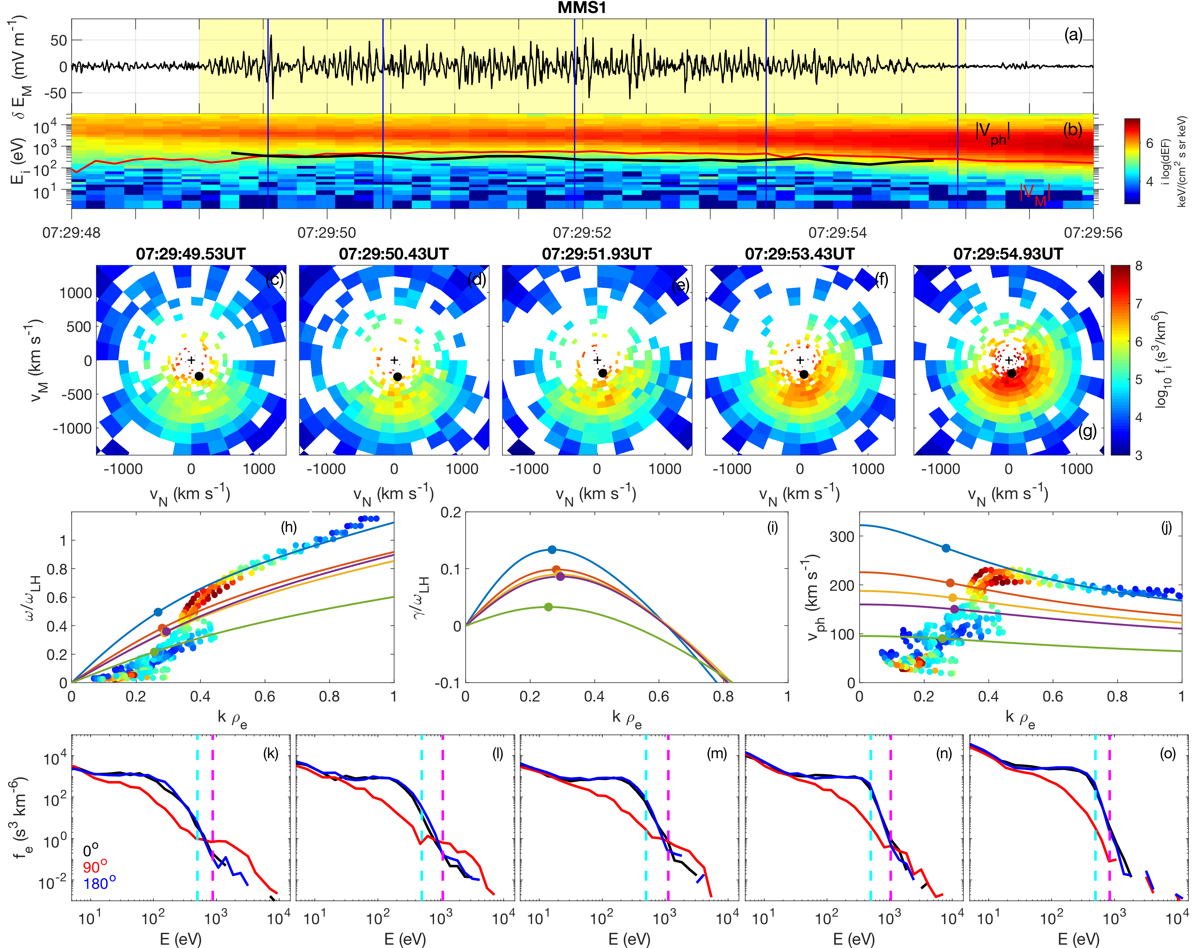
Figure 10: Ion and electron distributions and MTSI dispersion relations based on MMS1 data when the lower hybrid waves are observed. (a) $\delta E_{M}$. (b) Ion differential energy flux. (c)–(g) Ion distributions in the $v_{N}$–$v_{M}$ plane perpendicular to ${\bf B}$ at the times indicated by the blue vertical lines in panels (a) and (b). The distributions are shown in the spacecraft frame (the plusses indicate zero velocity and the circles indicate ${\bf v}_{ph}$ around the time the ion distributions are observed). (h)–(j) Frequencies, growth rates, and phase speeds versus $k$, respectively, based on the ion distributions in panels (c) blue, (d) red, (e) gold, (f) purple, and (g) green. The dispersion relations are found by solving equation (7) using the parameters in Table 1. We also plot the results from Figure 5 in panels (h) and (i). (k)–(o) Electron pitch-angle distributions measured by MMS1 at the same time as the ion distributions in panels (c)–(g), respectively. The phase-space densities $f_{e}$ are plotted as a function of $E$ for pitch angles $\theta=0^{\circ}$ (black), $90^{\circ}$ (red), and $180^{\circ}$. The magenta dashed lines indicate the parallel resonant parallel energies calculated from the predicted dispersion relations in panels (h)–(j). The cyan lines indicate $v_{\parallel}=500$ eV estimated from equation (6).

The parallel resonant energies $v_{\parallel}=\omega/k_{\parallel}$ are $\sim 1\,\mathrm{keV}$ for the 5 cases, based on the predicted wave properties in Figure 10. The values of $v_{\parallel}$ only depend weakly on $\theta_{kB}$ over the range of $\theta_{kB}$ where $\gamma_{\mathrm{max}}>0$ is found. This value is in good agreement with $v_{\parallel}\sim 500$ eV, estimated in section 4.3. Therefore, the predicted resonant energies are above the thermal energies of the electrons ($\sim 100-250\,\mathrm{eV}$). Figures 10k–10o show the electron phase-space densities $f_{e}$ at pitch angles $\theta=0^{\circ}$, $90^{\circ}$, and $180^{\circ}$ at times corresponding to cases 1–5 in Table 1. In each case a clear temperature anisotropy $T_{\parallel}/T_{\perp}>1$ occurs for the thermal electron population. In Figures 10m–10o, $f_{e}$ at $\theta=0^{\circ}$ and $180^{\circ}$ are characterized by approximately flat-top distributions over a wide range of energies, consistent with trapping and acceleration by large-scale parallel electric fields. The distributions are nearly identical to those found in the magnetospheric inflow regions of magnetopause reconnection Graham et al. (2014, 2016a); Wang et al. (2017). Figures 10k–10o show that the parallel resonant energies associated with the lower hybrid waves are above the energy range of the flat-top $f_{e}$, suggesting that the observed waves are not directly responsible for electron heating in the thermal energy range. In this case the wavelengths are too large to directly interact with the thermal population. If any shorter wavelength waves develop and contribute to the observed parallel electron heating, they are likely quickly dissipated.

The distributions in Figures 10m–10o are observed in the interval where high-frequency electrostatic waves are seen in Figure 3. The approximately flat-top distributions for $\theta=0^{\circ}$ and $180^{\circ}$ suggests marginal stability. Therefore, any modifications to the distributions resulting in beam-like features are potentially unstable to parallel streaming instabilities, resulting in the observed high-frequency electrostatic waves. Once generated, the effect of the waves is to return the distribution to the marginally stable flat-top distribution Egedal et al. (2015). This scenario accounts for the simultaneous observation of the flat-top distributions and high-frequency electrostatic waves over an extended interval.

In Figures 10k–10m we observe a hot electron distribution for $\theta=90^{\circ}$ corresponding to the enhancement of hot electron fluxes in Figure 2j. In Figures 10k and 10l there is evidence of a positive slope in $f_{e}$ at $\theta=90^{\circ}$, suggesting that ring distributions are developing. At these energies there is negligible $f_{e}$ at $\theta=0^{\circ}$ and $180^{\circ}$, so we do not expect these distributions to develop as a result of wave-particle interactions, although the distributions only develop when the lower hybrid waves are observed. This may suggest that the high-energy electron fluxes are enhanced as a result of large-scale electric fields, possibly set up by the finite-gyroradius effect of the magnetosheath ions.

In summary, we investigated the lower hybrid waves at an extended magnetopause crossing. The electron velocity and density fluctuations associated with the lower hybrid waves are resolved. The spacecraft separations are sufficiently small that the phase speed and propagation direction of the lower hybrid waves can be determined using four-spacecraft timing of the electric and magnetic field fluctuations. We find excellent agreement between the four-spacecraft timing and single-spacecraft methods for determining the lower hybrid wave properties. Comparison of observations with linear theory shows that the lower hybrid waves are consistent with generation by MTSI due to the cross-field ion drift associated with the finite gyroradius magnetosheath ions entering the magnetosphere. This suggests that these ion distributions, which are often associated with asymmetric reconnection, are unstable and generate lower hybrid waves.

5 14 December 2015

In this section we investigate the lower hybrid waves observed near the EDR encounter on 14 December 2015 observed at approximately 01:17:40 UT Graham et al. (2017b); Ergun et al. (2017); Chen et al. (2017). In Ergun et al. (2017) the waves observed close to the neutral point were interpreted as a long wavelength corrugation of the current sheet. Here, we reinvestigate the wave properties using the highest resolution electron moments and compare the results with the lower hybrid waves observed in section 4.

5.1 Overview

For this magnetopause crossing the spacecraft were located at [10.1, -4.3, -0.8] $R_{E}$ (GSE) and separated by $\sim 15\,\mathrm{km}$. We rotate the vector quantities into an LMN coordinate system given by ${\bf L}=[0.02,-0.52,0.86]$, ${\bf M}=[-0.51,-0.74,-0.44]$, ${\bf N}=[0.86,-0.43,-0.27]$ in GSE coordinates. Based on timing analysis of $B_{L}$ we estimate the magnetopause boundary velocity to be $\approx 35\times[-0.28,-0.10,0.96]\,\mathrm{km}\,\mathrm{s}^{-1}$ (LMN). This reconnection event has a relatively small guide-field, $\sim 30\%$ of the reconnection magnetic field. Figures 11a–11c provide an overview of the reconnection event from MMS3, which crosses the magnetopause from the magnetosheath to the magnetosphere. At the beginning of the interval the spacecraft is in the southward reconnection outflow. The spacecraft crosses the current sheet neutral point at about 01:17:40.0 UT where $B_{L}=0$ (indicated by the magenta vertical dashed line) and then enters the magnetospheric inflow region. Around this region agyrotropic electron distributions are observed, indicating close proximity to the electron diffusion region Graham et al. (2017b). Like previous observations, the magnetospheric inflow region is characterized by increased electric field fluctuations near $f_{LH}$ and parallel electron heating (not shown). On the magnetospheric side of the magnetopause we observed both hot ($E\gtrsim 1$ keV) and colder ($E\lesssim 1$ keV) electron populations in Figure 11c. The colder magnetosheath population tends to increase in temperature and decrease in density toward the magnetosphere within the yellow-shaded interval in Figure 11.

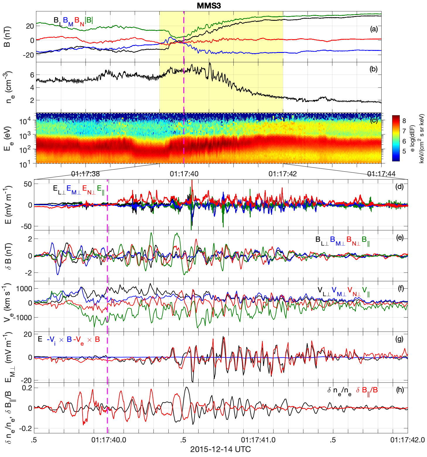
Figure 11: Overview of the magnetopause crossing observed on 14 December 2015 observed by MMS3. (a) ${\bf B}$ (Combined FGM/SCM data). (b) $n_{e}$ (133 Hz data). (c) Electron omni-direction differential energy flux. Panels (d)–(h) show properties of the lower hybrid waves in the yellow-shaded region in panels (a)–(c). (d) Perpendicular and parallel components of ${\bf E}$. (e) Parallel and perpendicular components of the fluctuating ($f>5$  Hz) magnetic field $\delta{\bf B}$. (f) Perpendicular and parallel components of ${\bf V}_{e}$. (g) $E_{M\perp}$ (black) and the M components of the ion and electron convection terms, $(-{\bf V}_{i}\times{\bf B})_{M}$ (blue) and $(-{\bf V}_{e}\times{\bf B})_{M}$ (red). (h) $\delta n_{e}/n_{e}$ (black) and $\delta B_{\parallel}/|{\bf B}|$ (red).

In the magnetospheric inflow region we observe large perturbations in ${\bf B}$ (Figures 11a and 11h) and $n_{e}$ (Figures 11b and 11h). The density perturbations are seen in the electron omnidirectional energy flux (Figure 11c). These perturbations are largest at the density gradient, suggestive of lower hybrid drift waves. Below we investigate the properties of the waves, in particular, their dispersion relation and wave-normal angle.

5.2 Lower hybrid wave properties

Figures 11d–11h show fields and particle observations in the yellow-shaded region of Figures 11a and 11b. Figure 11d shows the components of ${\bf E}$ perpendicular and parallel to ${\bf B}$. Large amplitude fluctuations are seen in all components of ${\bf E}$. Lower frequency fluctuations are seen in ${\bf E}_{\perp}$, and higher frequency ${\bf E}_{\parallel}$ are also observed. In addition, there is a large-scale Hall electric field $E_{N}>0$. Here, lower hybrid fluctuations are seen in $E_{M\perp}$ and $E_{L\perp}$ due to the guide-field.

Figure 11e shows that $\delta{\bf B}$ is primarily aligned with ${\bf B}$ and is largest amplitude when the $E_{M\perp}$ and $E_{L\perp}$ fluctuations are observed. We also observe significant $\delta B_{N\perp}$, consistent with a finite $k_{\parallel}$. Large-amplitude $\delta{\bf B}$ are also observed on the magnetosheath side of the neutral point, where ${\bf E}$ is small. Close to the neutral point between 01:17:40.0 UT and 01:17:40.4 UT there are fluctuations in $E_{N\perp}$ and $\delta B_{\parallel}$. These fluctuations are inconsistent with the usual lower hybrid wave predictions.

Figure 11f shows perpendicular and parallel components of ${\bf V}_{e}$. Large fluctuations in $V_{N\perp}$ are observed, consistent with lower hybrid waves. We also observe large fluctuations in $V_{\parallel}$, indicating a finite $k_{\parallel}$, and some fluctuations in $V_{L\perp}$ and $V_{M\perp}$. In addition, we observe large-scale parallel and perpendicular $V_{e}$ associated with the current sheet. In Figure 11g we plot $E_{M\perp}$ and the ${\bf M}$ components of the ion and electron convection terms, $(-{\bf V}_{i}\times{\bf B})_{M}$ and $(-{\bf V}_{e}\times{\bf B})_{M}$, respectively. Throughout the interval ${\bf E}_{\perp}\approx-{\bf V}_{e}\times{\bf B}$ meaning electrons remain approximately frozen in. In contrast, $-{\bf V}_{i}\times{\bf B}$ remains close to zero (although the sampling rate for ions only partially resolves the lower hybrid fluctuations). We interpret these fluctuations in $E_{M}$ between 01:17:40.4 UT and 14:17:41.5 UT as lower hybrid waves.

In Figure 11h we plot $\delta n_{e}/n_{e}$ and $\delta B_{\parallel}/B$, where the fluctuating quantities are assumed to have $f>5$ Hz. Both quantities reach maximum values of $\approx 0.2$. The largest $\delta n_{e}/n_{e}$ are colocated with largest $E_{M\perp}$, suggesting that the density perturbations are associated with the lower hybrid waves on the lower-density side of the current sheet. In contrast, $\delta B_{\parallel}/B$ become larger as the plasma becomes more weakly magnetized and are largest near the center of the current sheet, where ${\bf B}$ is close to the ${\bf M}$ direction. Thus, at low densities $(\delta n_{e}/n_{e})/(\delta B_{\parallel}/B)>1$, while at higher densities $(\delta n_{e}/n_{e})/(\delta B_{\parallel}/B)<1$. While this trend is qualitatively consistent with cold plasma predictions, the gradients in $n$ and $B$ will modify the predictions (see Appendix A). We find that $\delta n_{e}$ and $\delta B_{\parallel}$ tend to be anticorrelated, where the lower hybrid waves are observed, while close to the neutral point $\delta n_{e}$ and $\delta B_{\parallel}$ are close to in phase. We note that since fluctuations in $E_{N\perp}$, $V_{L\perp}$ and $V_{M\perp}$ are observed, the waves are non-planar, and possibly vortex-like structures Tanaka and Sato (1981); Norgren et al. (2012); Price et al. (2016). We conclude that the waves observed between 01:17:40.4 UT and 01:17:41.5 UT on MMS3 are lower hybrid waves.

For this event we can investigate whether the differences between ${\bf E}$ and $-{\bf V}_{e}\times{\bf B}$ are due to electron pressure fluctuations associated with the observed $\delta n_{e}/n_{e}$. The electron momentum equation is given by

$${\bf E}+{\bf V}_{e}\times{\bf B}=-\frac{\nabla\cdot{\bf P}_{e}}{ne}-\frac{m_{e}}{e}\left[\frac{\partial{\bf V}_{e}}{\partial t}+\left({\bf V}_{e}\cdot\nabla\right){\bf V}_{e}\right],$$ (8)

where ${\bf P}_{e}$ is the electron pressure tensor. We can estimate the pressure divergence term in the ${\bf M}$ direction with a single-spacecraft method using $-\nabla\cdot{\bf P}_{e}/ne\approx-\nabla P_{e,\perp}/ne\approx(nev_{ph})^{-1}\partial P_{e,\perp}/\partial t$, where $v_{ph}$ is the speed of the pressure fluctuations past the spacecraft in the ${\bf M}$ direction, and $P_{e,\perp}$ is the perpendicular electron pressure. We use $v_{ph}=220$ km s^-1, which is determined by the best fit of $-\nabla P_{e,\perp}/ne$ to ${\bf E}+{\bf V}_{e}\times{\bf B}$. This provides an estimate of $v_{ph}$ for the waves. This $v_{ph}$ is calculated in the spacecraft frame, which approximately corresponds to the ion stationary frame.

In Figure 12a we plot the ${\bf M}$ components of ${\bf E}$, $-{\bf V}_{e}\times{\bf B}$, and $-\nabla P_{e,\perp}/ne$. We find that $-\nabla P_{e,\perp}/ne$ reaches large amplitudes ($>10$ mV m^-1) while the waves are observed, and in some places is comparable in magnitude to ${\bf E}$ and $-{\bf V}_{e}\times{\bf B}$. In general, $-\nabla P_{e,\perp}/ne$ is out of phase with both ${\bf E}$ and $-{\bf V}_{e}\times{\bf B}$ when the waves are observed. This results in some phase difference between ${\bf E}$ and $-{\bf V}_{e}\times{\bf B}$, while the relative amplitudes of ${\bf E}$ and $-{\bf V}_{e}\times{\bf B}$ remain comparable. In Figure 12b we plot the ${\bf M}$ components of ${\bf E}+{\bf V}_{e}\times{\bf B}$ and $-\nabla P_{e,\perp}/ne$. Overall, we find that ${\bf E}+{\bf V}_{e}\times{\bf B}\approx-\nabla P_{e,\perp}/ne$, which is most clearly seen between 01:17:40.5 UT and 01:17:41.0 UT. The amplitudes and phases are similar, indicating that the pressure fluctuations associated with the waves can account for the observed differences between ${\bf E}$ and $-{\bf V}_{e}\times{\bf B}$.

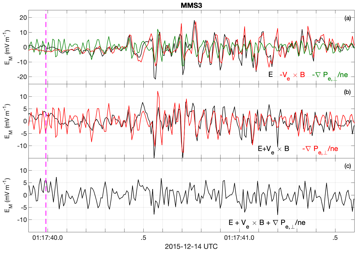
Figure 12: Terms in the electron momentum equation for lower hybrid waves observed by MMS3. (a) ${\bf M}$ components of ${\bf E}$ (black), $-{\bf V}_{e}\times{\bf B}$ (red), and $-\nabla P_{e,\perp}/ne$ (green). (b) ${\bf M}$ components of ${\bf E}+{\bf V}_{e}\times{\bf B}$ (black) and $-\nabla P_{e,\perp}/ne$ (red). (c) ${\bf M}$ component of ${\bf E}+{\bf V}_{e}\times{\bf B}+\nabla P_{e,\perp}/ne$. The magenta line indicates when $B_{L}=0$.

In Figure 12c we plot the ${\bf M}$ component of ${\bf E}+{\bf V}_{e}\times{\bf B}+\nabla P_{e,\perp}/ne$. We find that this quantity fluctuates with amplitudes of $\sim 5$ mV m^-1, typically smaller than the values of ${\bf E}$, $-{\bf V}_{e}\times{\bf B}$, and $-\nabla P_{e,\perp}/ne$. This quantity provides an indicator of the overall uncertainties, rather than the values of the remaining terms in equation (8). The main sources of uncertainty are: (1) ${\bf E}$ is down-sampled to the cadence of the electron moments, (2) ${\bf V}_{e}$ and ${\bf P}_{e}$ are computed from distributions with reduced angular coverage Rager et al. (2018), and (3) the pressure divergence terms must be approximated using the single-spacecraft method. For comparison, rough estimates of the remaining terms in equation (8) [not shown] yield values less than $1$ mV m^-1, and are thus unlikely to account for the fluctuations in Figure 12c. For this example, we conclude that deviations of ${\bf E}$ from $-{\bf V}_{e}\times{\bf B}$ result from fluctuations in ${\bf P}_{e}$ associated with the waves, and to a lesser extend the uncertainties associated with the measurements of ${\bf E}$ and the electron moments.

We now investigate the wave properties in more detail. Figure 13 shows the calculated $\delta\phi_{B}$ using equation (5) and the best fit of $\delta\phi_{E}$ to $\delta\phi_{B}$ for MMS1–MMS4, respectively. For reference, $B_{L}=0$ is indicated by the vertical magenta lines in each panel. To compute $\delta\phi_{B}$ and $\delta\phi_{E}$ we bandpass ${\bf B}$ and ${\bf E}$ between $5\,\mathrm{Hz}$ and $100\,\mathrm{Hz}$, which corresponds to the frequencies where the wave power is maximal. For each spacecraft we find good correlations between $\delta\phi_{E}$ to $\delta\phi_{B}$ throughout the interval. We find that the maximum wave potentials are $\delta\phi_{\mathrm{max}}\approx 50\,\mathrm{V}$ on each spacecraft, corresponding to $e\delta\phi_{\mathrm{max}}/k_{B}T_{e}\sim 0.6$. In each case the largest $\delta\phi$ are found on the low-density side of the neutral point and $\delta\phi$ becomes negligible as the neutral point is approached. Thus, quasi-electrostatic lower hybrid waves do not penetrate into the electron diffusion region.

We note that the waveforms of $\delta\phi_{B}$ and $\delta\phi_{E}$ differ significantly for each spacecraft, prohibiting multi-spacecraft timing analysis of the waves to determine their properties. Based on the magnetopause boundary speed the lower hybrid waves occupy a width of $\sim 50\,\mathrm{km}$, corresponding to $\sim 0.7d_{i}$ (consistent with Pritchett et al. (2012)), where $d_{i}\approx 70\,\mathrm{km}$ is the magnetosheath ion inertial length. The most intense lower hybird waves occur at $\gtrsim 12$ km $=0.2$ $d_{i}$ from the neutral point.

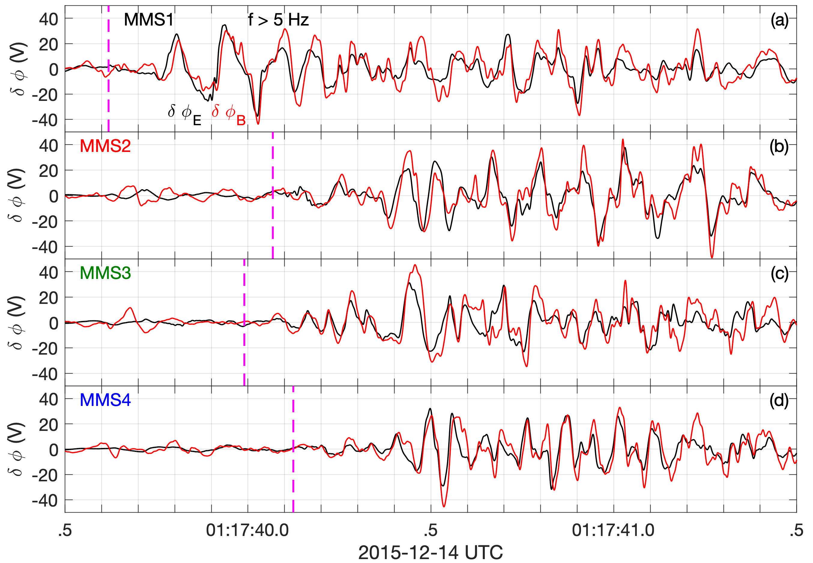
Figure 13: Lower hybrid waves observed in the magnetospheric inflow region observed by the four spacecraft. (a)–(d) $\phi_{B}$ (red) and the best fit of $\delta\phi_{E}$ (black) to $\delta\phi_{B}$ for MMS1–4, respectively. Fluctuating ${\bf E}$ and ${\bf B}$ are obtained for $f>5\,\mathrm{Hz}$. The lower hybrid wave properties are summarized in Table 2. The magenta dashed lines indicate the neutral point where $B_{L}=0$ for each spacecraft.

The lower hybrid wave properties determined from the analysis in Figure 13 are summarized in Table 2 for each spacecraft. Even though the waveforms differ significantly the estimated properties are very similar on each spacecraft. We find that the waves propagate in the ${\bf M}$ direction (dawnward), corresponding to the direction of both the large-scale ${\bf E}\times{\bf B}$ drift and electron diamagnetic drift (shown below). The lower hybrid waves are predicted to propagate approximately perpendicular to ${\bf B}$, so their propagation direction is oblique to the out-of-plane direction, due to the guide field in this event. On average we find that the waves have $v_{ph}\approx 160\,\mathrm{km}\,\mathrm{s}^{-1}$, slightly smaller than the estimate from the fluctuations in ${\bf P}_{e}$. We calculate $f\approx 13\,\mathrm{Hz}$ for the lower hybrid waves based on the power spectra of $E_{M}$ over the interval the waves are observed. We estimate the wavelength $\lambda\approx 12$ km, which is smaller than the spacecraft separations, accounting for the lack of correlation between $\delta\phi_{E}$ (and $\delta\phi_{B}$) observed by the different spacecraft. From this $\lambda$ we estimate $k\rho_{e}\sim 0.6$, corresponding to quasi-electrostatic lower hybrid waves, consistent with the predictions for lower hybrid waves in the electrostatic limit, and in agreement with previous observations Khotyaintsev et al. (2016); Graham et al. (2017a). This supports the conclusion that the fluctuations in ${\bf E}$, ${\bf B}$, ${\bf V}_{e}$ and $n_{e}$ observed on the low-density side of the neutral point are primarily due to lower hybrid waves.

MMS	v $(\mathrm{km}\,\mathrm{s}^{-1})$	direction (LMN)	$C_{\phi}$	$\lambda$ (km)
1	$144$	[0.47, 0.81, 0.35]	$0.78$	$11$
2	$172$	[0.66, 0.74, 0.12]	$0.84$	$13$
3	$162$	[0.56, 0.57, 0.60]	$0.72$	$12$
4	$166$	[0.66, 0.73, 0.21]	$0.78$	$13$

Table 2: Properties of the lower hybrid waves observed in the ion diffusion region on 14 December 2015. The properties are calculated for electric and magnetic field fluctuations above $5\,\mathrm{Hz}$.

We now compare the fields and electron energy densities of the lower hybrid waves using MMS3 in Figure 14. Figure 14b shows that for these waves most of the field energy density is in ${\bf B}$ since $cB/E>1$, thus $W_{f}\approx W_{B}$. Figures 14c and 14d show spectrograms of $W_{f}$ and $W_{e}$. Both spectrograms are similar, with most of the energy density being found close to but below $f_{LH}$ on the low-density side of the neutral point. Figure 14e shows that for $f<f_{LH}$ there is more energy density in the fields than electrons, in contrast to the 28 November 2016 event (Figure 4). This occurs because the waves have a smaller $k_{\perp}d_{e}$ (Figure 1f). Figure 14f shows the spectrogram of $\lambda$ using equation (4). For the lower hybrid waves shown in Figure 14a we estimate $\lambda\sim 10-20$ km, which agrees well with the results in Table 2.

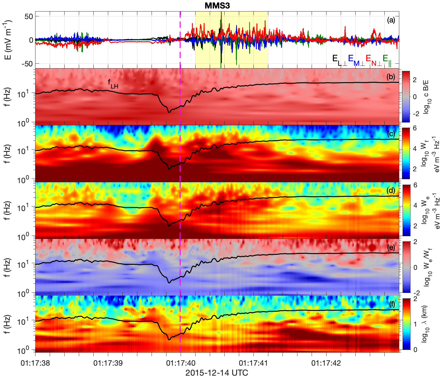
Figure 14: Properties of the lower hybrid waves observed on 14 December 2015 by MMS3. (a) Perpendicular and parallel components of ${\bf E}$. (b) Spectrogram of $cB/E$. (c) Spectrogram of $W_{f}$. (d) Spectrogram of $W_{e}$. (e) Spectrogram of $W_{e}/W_{f}$. (f) Spectrogram of $\lambda$.

In Figure 15a we plot the dispersion relations from the four spacecraft using equation (3). For MMS3 we take the median over the time interval indicated by the yellow-shaded region in Figure 14a, where the $E_{M\perp}$ fluctuations are observed. We use similarly long time intervals for the remaining spacecraft, although the start and end times differ because the spacecraft cross the neutral point and region with lower hybrid waves at different times. All four spacecraft yield similar results. The lower hybrid waves are characterized by $0.5\lesssim k_{\perp}\rho_{e}\lesssim 0.7$ (corresponding to $k_{\perp}d_{e}\approx 1$) and frequencies of $0.5\lesssim\omega/\omega_{LH}\lesssim 1$, or equivalently $8$ Hz $\lesssim f\lesssim 16$ Hz. This smaller $k_{\perp}d_{e}$ accounts for the smaller $W_{e}/W_{f}$ observed here compared with the 28 November 2016 event (cf., Figure 1f). From Figure 15b we estimate 100 km s${}^{-1}\lesssim v_{ph}\lesssim 250$ km s^-1, which agrees with the results in Table 2 and the value estimated from the fluctuations in ${\bf P}_{e}$. Compared with Figure 5b we find a much broader range of $v_{ph}$, which is likely because the waves here are more broadband in frequency. In addition, the spacecraft separation is larger here compared with $\lambda$, resulting in larger differences in the dispersion relations between each spacecraft.

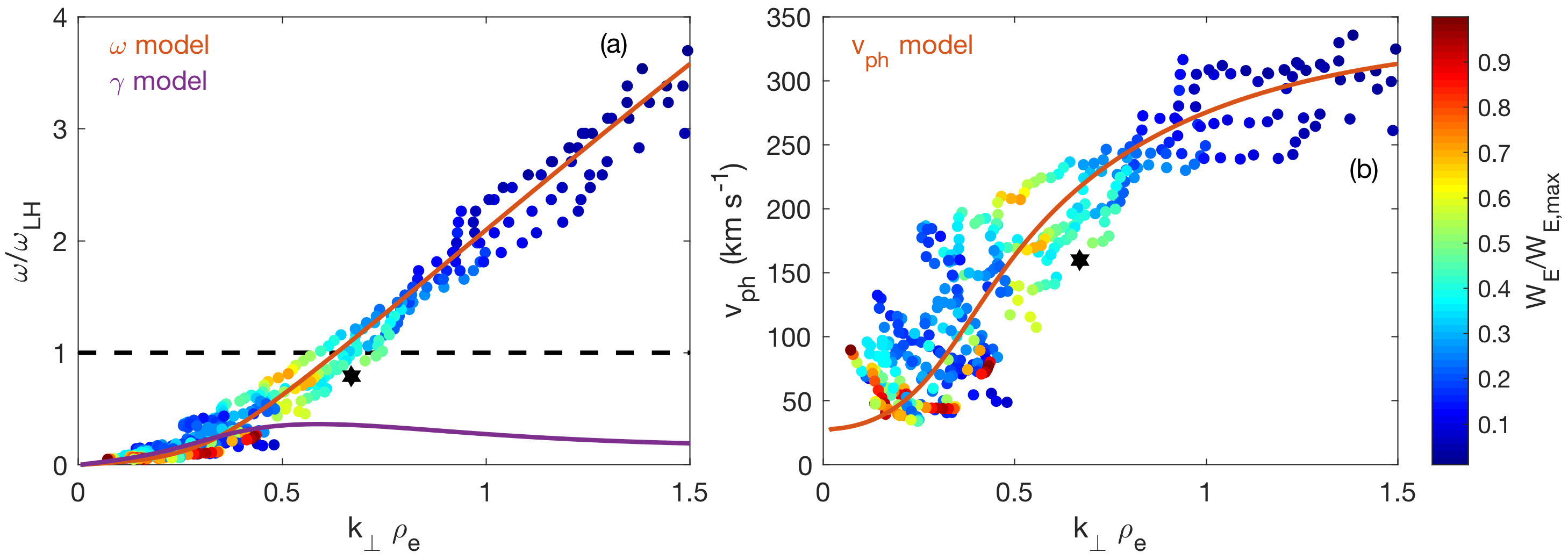
Figure 15: Dispersion relation of lower hybrid waves calculated using equation (3) for all four spacecraft. (a) Dispersion relations of the lower hybrid waves observed in the yellow-shaded region of Figure 14a. The black dashed lined indicates $\omega/\omega_{LH}=1$. The red and purple lines are the dispersion relation and growth rate calculated using equation (12). (b) Phase speed $v_{ph}$ versus $k_{\perp}\rho_{e}$. The black stars in panels (a) and (b) are the averages of the wave properties estimated in Table 2.

We now estimate $k_{\parallel}$ and $\theta_{kB}$ for these waves using $\delta B_{\parallel}/\delta B$, $\delta V_{e,\parallel}/V_{e,\perp}$, and $(\delta n_{e}/n_{e})/(\delta B/B)$. Figures 16a–16c show $\delta B_{\parallel}/\delta B$, $\delta V_{e,\parallel}/V_{e,\perp}$, and $(\delta n_{e}/n_{e})/(\delta B/B)$ versus $k_{\parallel}$ and $k_{\perp}$ predicted from homogeneous theory. We use $f_{pe}/f_{ce}=30$, corresponding to the median $f_{pe}/f_{ce}$ over the interval used to calculate the dispersion relations. We note that $f_{pe}/f_{ce}$ varies with position here so the estimates of $k_{\parallel}$ and $\theta_{kB}$ are approximate. We find that the lower hybrid waves have $k_{\perp}d_{e}\approx 1$, indicated by the vertical green lines in Figures 16a–16c.

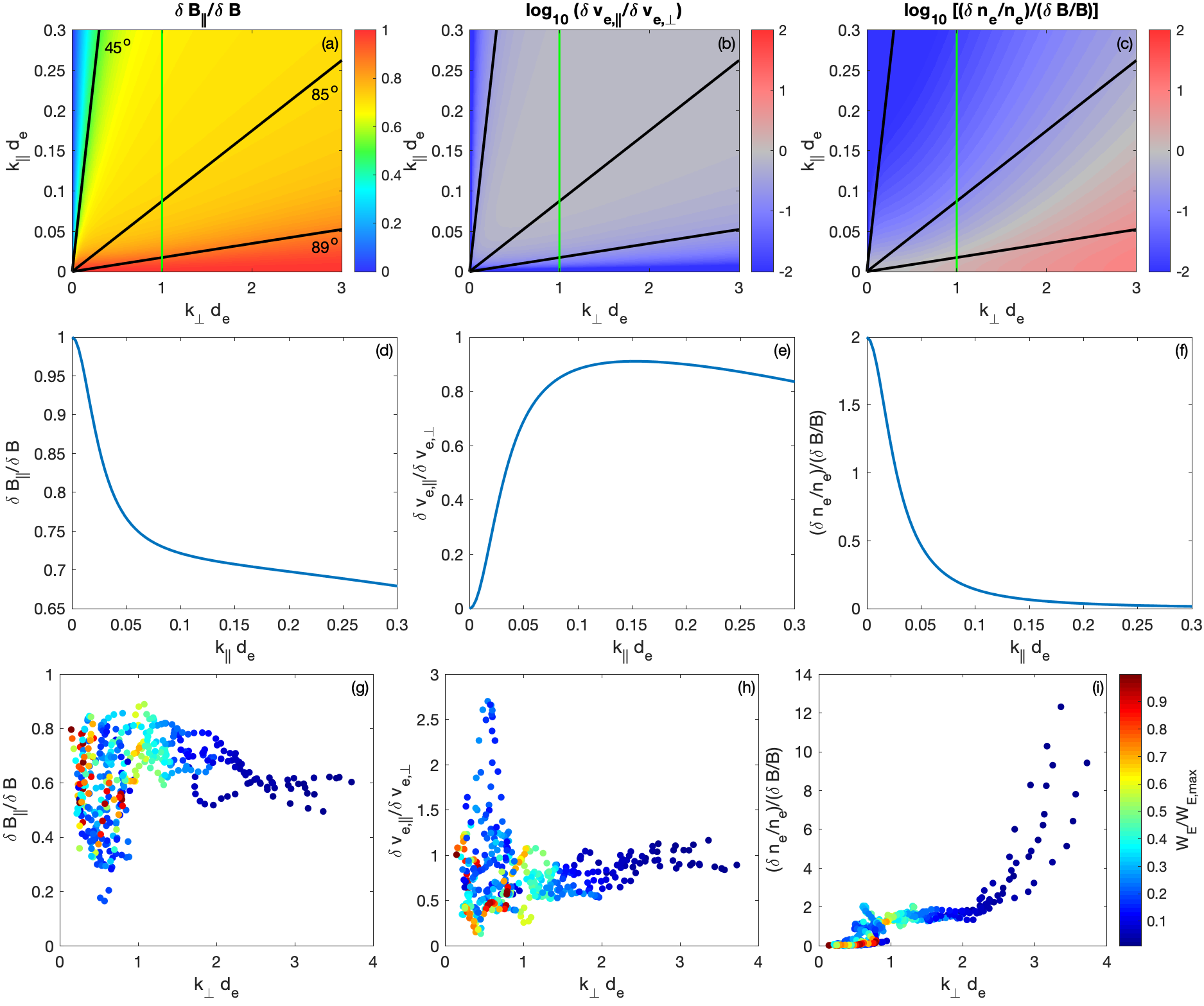
Figure 16: Estimates of the wave-normal angle and $k_{\parallel}$ from fields and particle observations of the lower hybrid waves observed 14 December 2015. (a)–(c) $\delta B_{\parallel}/\delta B$, $\delta V_{e,\parallel}/V_{e,\perp}$, and $(\delta n_{e}/n_{e})/(\delta B/B)$ for whistler/lower hybrid waves versus $k_{\parallel}$ and $k_{\perp}$. We use $f_{pe}/f_{ce}=30$. The green line is $k_{\perp}d_{e}=1$, the estimate $k_{\perp}$ of the observed waves. (d)–(f) $\delta B_{\parallel}/\delta B$, $\delta V_{e,\parallel}/V_{e,\perp}$, and $(\delta n_{e}/n_{e})/(\delta B/B)$ versus $k_{\parallel}d_{e}$ for $k_{\perp}d_{e}=1$. (g)–(i) Observed $\delta B_{\parallel}/\delta B$, $\delta V_{e,\parallel}/V_{e,\perp}$, and $(\delta n_{e}/n_{e})/(\delta B/B)$ of the lower hybrid waves versus $k_{\perp}d_{e}$.

In Figures 16d–16f we plot $\delta B_{\parallel}/\delta B$, $\delta V_{e,\parallel}/\delta V_{e,\perp}$, and $(\delta n_{e}/n_{e})/(\delta B/B)$ versus $k_{\parallel}d_{e}$ for $k_{\perp}d_{e}=1$. Qualitatively, the dependence of $\delta B_{\parallel}/\delta B$ and $\delta V_{e,\parallel}/V_{e,\perp}$ on $k_{\parallel}$ are very similar to the 28 November 2016 case, where $f_{pe}/f_{ce}$ is much smaller. In contrast, a substantially smaller $(\delta n_{e}/n_{e})/(\delta B/B)$ is predicted here because $\delta{\bf B}$ increases as $f_{pe}/f_{ce}$ increases. In Figures 16g–16i we plot $\delta B_{\parallel}/\delta B$, $\delta V_{e,\parallel}/V_{e,\perp}$, and $(\delta n_{e}/n_{e})/(\delta B/B)$ obtained from the four spacecraft versus $k_{\perp}d_{e}$. For $\delta B_{\parallel}/\delta B$ we obtain values of $0.6-0.9$, with an average of $\approx 0.75$ around $k_{\perp}d_{e}=1$, corresponding to $k_{\parallel}d_{e}\approx 0.06$ in Figure 16d. For $\delta V_{e,\parallel}/\delta V_{e,\perp}$ we obtain $0.3-1.0$, with an average of $0.7$ around $k_{\perp}d_{e}=1$, corresponding to $k_{\parallel}d_{e}\approx 0.05$ in Figure 16e. For $(\delta n_{e}/n_{e})/(\delta B/B)$ we obtain $1-2$, which is consistent with the predictions in Figure 16f. Here, $n_{e}$ is much larger than in Figure 6, so the spectrum of $\delta n_{e}/n_{e}$ should be more reliable. From the average of $(\delta n_{e}/n_{e})/(\delta B/B)$ around $k_{\perp}d_{e}=1$ we obtain $1.3$, corresponding to $k_{\parallel}d_{e}\approx 0.02$. This $k_{\parallel}d_{e}$ is smaller than the predictions from $\delta B_{\parallel}/\delta B$ and $\delta V_{e,\parallel}/\delta V_{e,\perp}$. We note that the values of $(\delta n_{e}/n_{e})/(\delta B/B)$ predicted from homogeneous theory are likely not valid here due to the dependence of $\delta n_{e}$ on the gradients in $n_{e}$ and $B$ (see Appendix A). The average $k_{\perp}d_{e}$ is then $\approx 0.05$, whence we calculate $\theta_{kB}\approx 87^{\circ}$. Thus, the estimated $\theta_{kB}$ is consistent with lower hybrid waves. The spread of data in Figures 16g–16i suggests that $\theta_{kB}$ may change with frequency or time/position. From $\theta_{kB}\approx 87^{\circ}$ we obtain a parallel resonant energy of $v_{\parallel}\sim 40$ eV. This $v_{\parallel}$ is below the local electron thermal energy, although there is a large uncertainty in the estimated $v_{\parallel}$. The estimated $v_{\parallel}$ is therefore not inconsistent with the waves interacting with the thermal electrons. In summary, the quantities $\delta B_{\parallel}/\delta B$ and $\delta V_{e,\parallel}/\delta V_{e,\perp}$ indicate that the lower hybrid waves have finite $k_{\parallel}$.

5.3 Cross-field drifts and instability analysis

To investigate the instability of the lower hybrid waves we study the force balance of the current sheet using the ion and electron momentum equations and investigate the nature of the associated cross-field particle drifts. The ion and electron pressure divergences are calculated from the four-spacecraft differences using the full ion and electron pressure tensors, ${\bf P}_{i}$ and ${\bf P}_{e}$, respectively. The large-scale electric field is found by resampling ${\bf E}$ to the cadence of the electron moments (30 ms) on each spacecraft and averaging the field over the four spacecraft. This sampling rate tends to under-resolve lower hybrid fluctuations. In addition, the four-spacecraft averaging tends to average out the lower hybrid waves because for this event the spacecraft separations are comparable or larger than the lower hybrid wavelength, Therefore, the computed terms approximate the non-fluctuating component of ${\bf E}$.

Figure 17 shows the results of the four-spacecraft analysis. Figure 17a shows the four-spacecraft averaged ${\bf B}$. Compared with Figure 11a most of the fluctuations have been removed. The parallel and perpendicular components of ${\bf J}$, shown in Figure 17b, are calculated using the Curlometer technique. This ${\bf J}$ approximates the large-scale non-fluctuating ${\bf J}$, because the spacecraft separations are too large to resolve $\delta{\bf J}$ intrinsic to the lower hybrid waves Graham et al. (2016a). The current density peaks close to the neutral point, rather than where the lower hybrid waves are observed. Comparable parallel and perpendicular ${\bf J}$ magnitudes (primarily in the ${\bf M}$ and ${\bf L}$ directions, except near the center of the current sheet) are observed in the yellow-shaded region, where the lower hybrid waves occur. On the magnetospheric side of the current sheet (yellow-shaded region) a large-scale normal electric field $E_{N}$ develops, typical of the ion diffusion region of magnetopause reconnection. In Figure 11d, $E_{N}$ is due to the large-scale Hall electric field and the fluctuations associated with the waves.

Neglecting anomalous terms, inertial terms, and temporal changes, the ion and electron momentum equations are

$${\bf E}+{\bf V}_{i}\times{\bf B}\approx\frac{\nabla\cdot{\bf P}_{i}}{ne},$$ (9)

$${\bf E}+{\bf V}_{e}\times{\bf B}\approx-\frac{\nabla\cdot{\bf P}_{e}}{ne},$$ (10)

respectively. Figures 17e and 17f show that these equations are approximately satisfied for ions and electrons, respectively. Moreover, we find that $\nabla\cdot{\bf P}_{i}\approx{\bf J}\times{\bf B}$, thus the cross-field current is produced by the ion pressure divergence to maintain force balance across the current sheet. In contrast, the electron pressure divergence has a much smaller contribution, due to the small $T_{e}/T_{i}$, yielding a maximum $-\nabla\cdot{\bf P}_{e}/ne\approx-2\,\mathrm{mV}\,\mathrm{m}^{-1}$ in the ${\bf N}$ direction on the magnetospheric side of the current sheet. This value is significantly smaller than the fluctuating component in the out-of-plane direction associated with the lower hybrid waves (Figure 12).

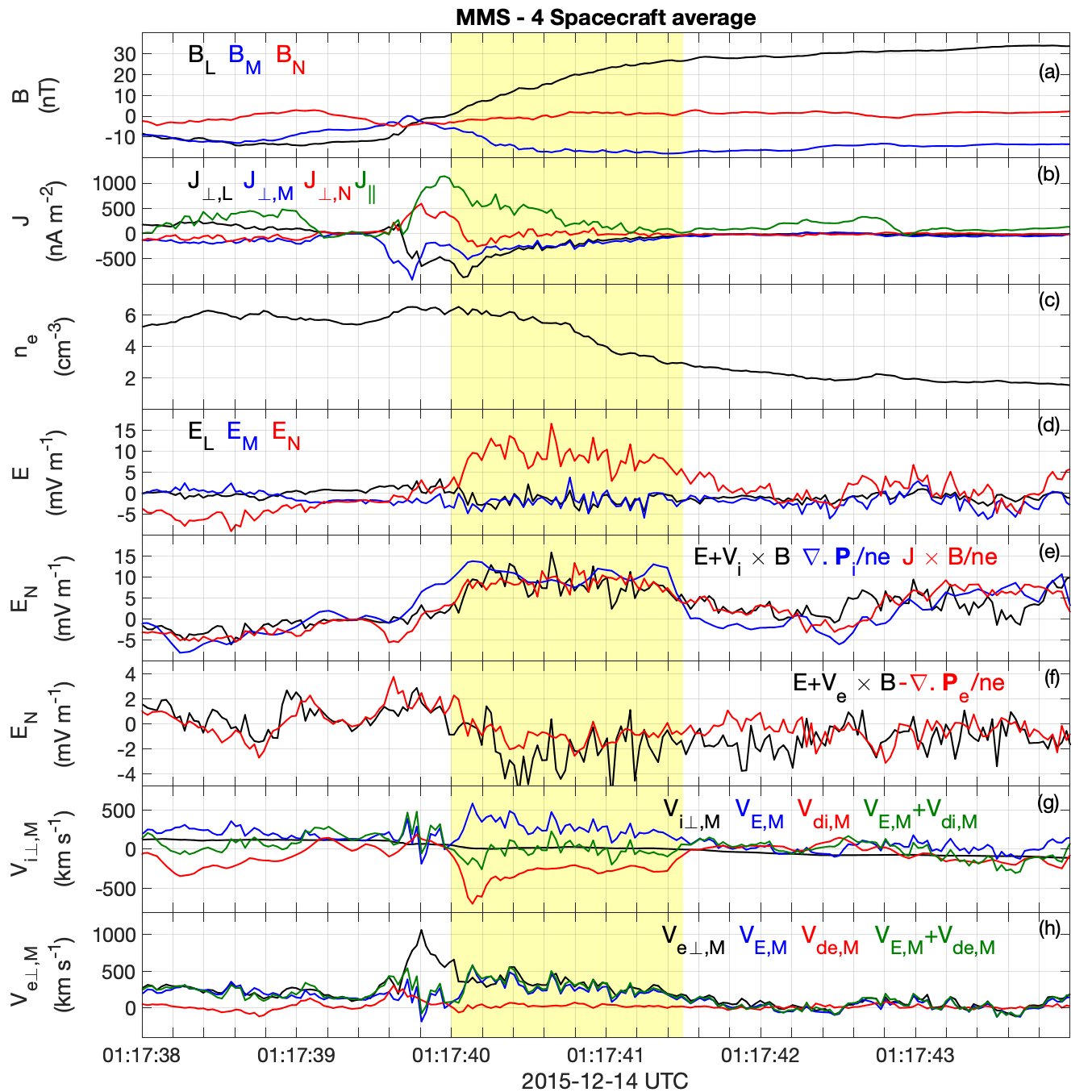
Figure 17: Large-scale fields and particle drifts obtained using four-spacecraft methods for the 14 December 2015 magnetopause crossing. (a) ${\bf B}$. (b) ${\bf J}$ computed using the Curlometer technique. (c) $n_{e}$. (d) ${\bf E}$. (e) ${\bf N}$ components of ${\bf E}+{\bf V}_{i}\times{\bf B}$ (black), $\nabla\cdot{\bf P}_{i}/ne$ (blue), and ${\bf J}\times{\bf B}/ne$. (f) ${\bf N}$ components of ${\bf E}+{\bf V}_{e}\times{\bf B}$ (black), $-\nabla\cdot{\bf P}_{e}/ne$ (blue). (g) ${\bf M}$ components of ion drifts perpendicular to ${\bf B}$; $V_{i\perp,y}$ (black), $V_{E,M}$ (blue), $V_{di,M}$ (red), and $V_{E,M}+V_{di,M}$ (green). (h) ${\bf M}$ components of electron drifts perpendicular to ${\bf B}$; $V_{e\perp,M}$ (black), $V_{E,M}$ (blue), $V_{de,M}$ (red), and $V_{E,M}+V_{de,M}$ (green).

By taking the cross products of equations (9) and (10) with ${\bf B}/B^{2}$ we obtain ${\bf V}_{i\perp}\approx{\bf V}_{E}+{\bf V}_{di}$ and ${\bf V}_{e\perp}\approx{\bf V}_{E}+{\bf V}_{de}$. Here ${\bf V}_{di}$ and ${\bf V}_{de}$ are the ion and electron diamagnetic drifts, given by

$${\bf V}_{di,e}=\pm\frac{{\bf B}\times\nabla\cdot{\bf P}_{i,e}}{B^{2}ne}.$$ (11)

In the out-of-plane direction we find that ${\bf V}_{i\perp}\approx{\bf V}_{E}+{\bf V}_{di}$ and ${\bf V}_{e\perp}\approx{\bf V}_{E}+{\bf V}_{de}$ are both approximately satisfied throughout the ion diffusion region, as seen in Figures 17g and 17h. For this event $V_{i\perp,M}\approx 0$, meaning $V_{E,M}\approx-V_{di,M}$. The cross-field current is therefore due to the ${\bf E}\times{\bf B}$ drift of electrons in the ${\bf M}$ direction.

At about 01:17:39.8 UT we find that ${\bf V}_{e\perp}\neq{\bf V}_{E}+{\bf V}_{de}$, likely because the EDR is observed around this time, which is smaller than the spacecraft separations. Therefore, the spacecraft separations may be too large to accurately compute $\nabla\cdot{\bf P}_{e}$ and spacecraft averaged quantities, thus the computed drifts may not be reliable here.

The results in Figure 17 are simply a consequence of the electron and ion momentum equations being satisfied in the limit when temporal changes and local acceleration can be neglected at ion spatial scales (larger than the typical lower hybrid wavelength). These results should not be particularly surprising, but they show that in the region where lower hybrid waves are observed, the cross-field current develops due to $\nabla\cdot{\bf P}_{i}$. Thus, the likely energy source of the observed waves is the cross-field current produced by $\nabla\cdot{\bf P}_{i}$, which can be unstable to LHDI.

To investigate the instability of the observed waves we consider the local dispersion equation for LHDI in the ion stationary frame Davidson et al. (1977)

$$0=1-\frac{\omega_{pi}^{2}}{k^{2}v_{i}^{2}}Z^{\prime}\left(\frac{\omega}{kv_{i}}\right)+\frac{\omega_{pe}^{2}}{\Omega_{ce}^{2}}\left(1+\frac{\omega_{pe}^{2}}{c^{2}k^{2}}\right)+\frac{2\omega_{pe}^{2}}{k^{2}v_{e}^{2}}\left(1+\frac{\beta_{i}}{2}\right)\frac{kV_{de}}{\omega-kV_{E}},$$ (12)

where ${\bf k}\cdot{\bf B}=0$. For the local plasma conditions we use $B=25\,\mathrm{nT}$, $n_{e}=5\,\mathrm{cm}^{-3}$, $T_{e}=90\,\mathrm{eV}$ and $T_{i}=500\,\mathrm{eV}$, and $V_{E}=-V_{di}=400\,\mathrm{km}\,\mathrm{s}^{-1}$, and $V_{de}=50\,\mathrm{km}\,\mathrm{s}^{-1}$, based on the median values over the interval the waves are observed. The effect of the weak pressure gradient is included through $V_{de}$.

Figure 15a shows the dispersion relation and growth rate, overplotted with the observed dispersion relations. The dispersion relation predicted by equation (12) is in excellent agreement with the observed dispersion relations. Similarly, the predicted $v_{ph}$, shown in Figure 15b is in excellent agreement with observations. For LHDI $\gamma_{\mathrm{max}}$ corresponds to $k_{\perp}\rho_{e}=0.6$, in agreement with where $W_{E}/W_{E,max}$ peaks. At $\gamma_{\mathrm{max}}$, $v_{ph}=190\,\mathrm{km}\,\mathrm{s}^{-1}$, which agrees with the observed dispersion relations and the value of $v_{ph}$ predicted in Figure 12, and is only slightly larger than values in table 2. Therefore, the LHDI predictions agree with observations so we conclude that the observed waves are produced by LHDI. However, close to the neutral point we expect equation (12) to become unreliable due to strong gradients in ${\bf B}$ and the neglect of electromagnetic effects.

In summary, the results show that the fluctuations in the ion diffusion region on the low-density side of the neutral point are consistent with lower hybrid drift waves. All the measured fluctuations, phase speed, dispersion relation and wave-normal angle are consistent with predictions for lower hybrid waves. We find that some deviation from the cold plasma predictions can occur due to the fluctuations in electron pressure associated with the waves and the density gradient where the waves occur. The single-spacecraft methods used to estimate the wave properties are in good agreement with each other. The primary free energy source of the lower hybrid waves is the ion pressure divergence, which is responsible for the cross-field current that excites the lower hybrid waves by LHDI.

6 Discussion

We have investigated in detail two examples of lower hybrid waves at the magnetopause. In both cases we find that the waves have $k\rho_{e}$ close to $0.5$ and frequencies $0.5\lesssim f/f_{LH}\lesssim 1$, consistent with quasi-electrostatic lower hybrid waves. Although in both examples the waves are consistent with lower hybrid waves, the waves have distinct electric field, magnetic field, and electron energy densities. These differences can be explained by cold plasma theory. For the 28 November 2016 event we find that the lower hybrid waves have $k_{\perp}d_{e}\approx 3$ for $f_{pe}/f_{ce}\approx 6.7$, and for the 14 December 2015 event we find $k_{\perp}d_{e}\approx 1$ and $f_{pe}/f_{ce}\approx 30$. We find that these differences account for the different wave properties between the two events. Specifically: (1) The value of $k_{\perp}d_{e}$ determines $W_{e}/W_{B}$ based on Figure 1f and equation (3), and accounts for the differences in $W_{e}/W_{B}$ between the two events. (2) As $f_{pe}/f_{ce}$ increases and/or $k_{\perp}d_{e}$ decreases, $cB/E$ is predicted to increase based on cold plasma predictions. This is due to the approximately frozen in motion of electrons, which is observed in both events. As $f_{pe}/f_{ce}$ increases $\delta{\bf J}$ is predicted to increase for a given $\delta{\bf E}$. This results in larger $\delta{\bf B}$ according to Ampere’s law, resulting in $cB/E$ increasing, which is consistent with the observed differences between the two events. In both events $\delta n_{e}/n_{e}$ are comparable, and reach peak values of $\delta n_{e}/n_{e}\approx 0.2$. Thus, the smaller $(\delta n_{e}/n_{e})/(\delta B/B)$ is due to the larger $\delta B/B$ observed on 14 December 2015. We conclude that the observed differences in lower hybrid waves properties in the two events are due to distinct $f_{pe}/f_{ce}$ and $k_{\perp}d_{e}$.

Another important difference between the two events is that on 14 December 2015 the waves were much more localized and the density gradient is more significant. Therefore, we need to consider the effect of gradients on the wave properties. Based on the continuity equation it is straightforward to show that

$$\delta n_{e}\approx\frac{nk_{\perp}}{B(\omega-k_{\perp}V_{e,M})}\left(\frac{n^{\prime}}{n}-\frac{B^{\prime}}{B}\right)\delta\phi,$$ (13)

when electrons are frozen in. Here the primes denote derivatives in the ${\bf N}$ direction. At Earth’s magnetopause, where the lower hybrid waves are observed, $n^{\prime}>0$ and $B^{\prime}<0$ and $\omega-k_{\perp}V_{e,M}<0$, so $\delta n_{e}$ is expected to be anticorrelated with $\delta\phi$. Thus, gradient terms may be the dominant contribution to $\delta n_{e}$. By substituting equation (5) into equation (13) we obtain:

$$(\delta n_{e}/n_{e})/(\delta B_{\parallel}/B)\approx\frac{f_{ce}}{f_{pe}}\frac{ck_{\perp}d_{e}}{(\omega-k_{\perp}V_{e,M})}\left(\frac{n^{\prime}}{n}-\frac{B^{\prime}}{B}\right).$$ (14)

Equation (14) predicts that $(\delta n_{e}/n_{e})/(\delta B_{\parallel}/B)$ increases toward the magnetopause as $f_{pe}/f_{ce}$ and $n^{\prime}/n-B^{\prime}/B$ increase. This is consistent with the observations in Figure 11, so we conclude that the gradients in $n$ and $B$ provide important contributions to $\delta n_{e}$. Finally, we note that the localization in the ${\bf N}$ direction will result in $\delta E_{N}$ because $\delta\phi^{\prime}\neq 0$. Since electrons are approximately frozen in $\delta V_{e,M}$ will also occur. These fluctuations are observed in Figure 11.

Our interpretation of these localized lower hybrid waves is that they correspond to the ripple structures found in three-dimensional simulations of asymmetric reconnection Pritchett and Mozer (2011); Pritchett et al. (2012); Pritchett (2013). In Pritchett et al. (2012) and Pritchett (2013) these ripple structures and the associated electric field fluctuations were interpreted as waves generated by LHDI. In addition, rippling waves have been found in simulations Pritchett and Coroniti (2010); Divin et al. (2015) and observations Pan et al. (2018) of dipolarization fronts in Earth’s magnetotail. In general, these ripples have been interpreted as resulting from LHDI or a closely related instability Pritchett and Coroniti (2010); Price et al. (2017).

The 14 December 2015 event was investigated in detail by Ergun et al. (2017). They investigated the waves at $7.5$ Hz near the neutral point. They found that the polarization properties were consistent with a corrugation of the current sheet, which explains the fluctuations in $\delta E_{N}$, $\delta n_{e}$, and $\delta B_{\parallel}$. They concluded that these waves were an electromagnetic drift wave, with phase speed of $\sim 600$ km s^-1 and wavelength $\sim 80$ km. These values of $v_{ph}$ and $\lambda$ are significantly larger than the values we calculate here for lower hybrid waves. Qualitatively, the main difference is that Ergun et al. (2017) predicts that the current sheet is corrugated, while here we interpret the fluctuations as smaller-scale ripples localized to the low-density side of the current sheet. However, both models predict very similar fluctuations in $\delta{\bf E}$, $\delta n_{e}$, and $\delta B_{\parallel}$, and thus both processes could be active at the current sheet; both processes may be manifestations of the same underlying instability.

The two events detailed in this paper show that the observed lower hybrid waves are consistent with generation by the lower hybrid drift instability (LHDI) and the closely related modified two-stream instability. Technically both instabilities are approximations to a more general dispersion equation for lower hybrid waves Hsia et al. (1979); Silveira et al. (2002). In addition to the instabilities investigated in sections 4 and 5, Graham et al. (2017a) found that when cold magnetospheric ions are present the ion-ion cross-field instability could develop between cold magnetospheric ions and finite gyroradius magnetosheath ions. The wave properties and propagation direction developing for this instability are similar to the MTSI predictions (without cold magnetospheric ions). The primary difference between the two instabilities is that the ion-ion cross-field instability is unstable for ${\bf k}\cdot{\bf B}=0$, due to the second ion population, whereas MTSI is stabilized. In either case the ion drift associated with the finite gyroradius magnetosheath ions provides the free energy of the lower hybrid waves. In both cases the waves propagate duskward in the cross-field ion drift direction, but at a slow speed than the bulk ion velocity of the magnetosheath ions. Therefore, in the frame of these ions, the waves propagate dawnward. The width of the region over which the instabilities can occur is determined by the gyroradius of magnetosheath ions, which is much larger than the predicted and observed wavelengths of the lower hybrid waves and thus the gradients can be weak, thus justifying the MTSI and local approximations. The results in section 4 suggest that finite gyroradius ion effects are not necessarily associated with the ion diffusion region of ongoing magnetic reconnection.

For magnetopause reconnection near the subsolar point we expect lower hybrid drift waves to be produced in the ion diffusion region by the ion pressure divergence. In such cases the ion diamagnetic drift velocity is approximately balanced by ${\bf E}\times{\bf B}$, resulting in negligible ion motion in the reconnection out-of-plane direction in the spacecraft frame. In contrast, the electrons propagate at approximately the ${\bf E}\times{\bf B}$ velocity, with a smaller contribution from electron diamagnetic drift in the same direction. As a result the lower hybrid drift waves propagate in the ${\bf E}\times{\bf B}$ and electron diamagnetic drift directions (dawnward). Thus, in the spacecraft frame the waves propagate the opposite direction to the waves associated with finite gyroradius ions.

In both cases we find that the lower hybrid waves have a finite $k_{\parallel}$, and can thus interact with thermal electrons via Landau resonance Cairns and McMillan (2005). The finite $k_{\parallel}$ is most evident from the fluctuations in the parallel electron velocity, and are observed in many other magnetopause crossings (not shown). From the estimates of the observed $k_{\parallel}$ we find that lower hybrid waves can interact with parallel propagating thermal and suprathermal electrons. The observed lower hybrid waves reach large amplitudes and can occur over an extended region, so they can plausibly contribute to the observed electron heating. Both events show wave potentials reaching $e\delta\phi_{\mathrm{max}}/k_{B}T_{e}\sim 0.5-1$. Similarly large potentials have been reported in other magnetopause reconnection events Khotyaintsev et al. (2016); Graham et al. (2017a). Future work is required to investigate the importance of lower hybrid waves for parallel electron heating. Parallel electron heating is expected in the ion diffusion region and magnetospheric inflow regions due to electron trapping (e.g., Egedal et al., 2011). In three-dimensional simulations when lower hybrid waves are excited, Le et al. (2017) found that parallel electron heating was further enhanced compared with the two dimensional case. However, the precise mechanisms and role of the lower hybrid waves in parallel electron heating were not clear.

7 Conclusions

In this paper we have investigated the properties and generation of lower hybrid waves at Earth’s magnetopause based on two case studies. For the first time we use electron moments, which resolve fluctuations at lower hybrid wave frequencies, to investigate the wave properties in unprecedented detail. The key results of this paper are:

(1) Electron number density and electron velocity fluctuations associated with lower hybrid waves are resolved. The electrons are shown to remain frozen in at frequencies where the amplitude of lower hybrid waves is maximal. Large parallel electron velocity fluctuations are observed, indicating that the waves have a finite parallel wave vector.

(2) The spectrogram of electron energy density associated with lower hybrid waves is computed and compared with energy density of the electric and magnetic field. The ratio of the electron to field energy density increases with frequency, consistent with theoretical predictions. The ratio of electron to magnetic field energy density is used to construct the dispersion relations of the waves, which are in excellent agreement with theoretical predictions.

(3) Comparison of the observed wave properties with theoretical predictions shows that the lower hybrid waves have a finite parallel wave number and wave-normal angle close to $89^{\circ}$. This allows lower hybrid waves to interact with thermal and suprathermal electrons, potentially contributing to parallel electron heating near the magnetopause. The estimated wave properties are in excellent agreement with the single-spacecraft method developed in Norgren et al. (2012).

(4) For spacecraft separations below the wavelength of lower hybrid waves, four-spacecraft timing analysis can be used to determine the wave properties. The phase speed and propagation directions agree very well with single-spacecraft methods, thus showing that when multi-spacecraft observations are unavailable the lower hybrid wave properties can be accurately determined from single-spacecraft observations.

(5) The observed waves are consistent with generation by the lower hybrid drift instability or the modified two-stream instability. In both cases the source of instability is the cross-field current at the magnetopause.

(6) The differences between lower hybrid wave properties, such as the ratio of magnetic field energy density to electric field energy density and the relative amplitudes of magnetic field and density fluctuations, are determined by the ratio of the electron plasma frequency to electron cyclotron frequency and the wave number. The ratio of field to particle energy densities is determined by the perpendicular wave number of the waves. These predictions are well approximated by cold plasma theory and account for the differences in lower hybrid wave properties observed at the magnetopause.

Appendix A Derivation of single spacecraft methods to determine lower hybrid wave properties

In this section we derive the equations used to determine the lower hybrid wave properties and dispersion relation using a single spacecraft. We also consider the sources of uncertainty in the methods used. To model the wave properties we make the following assumptions: (1) The waves are quasi-electrostatic. (2) Electrons are frozen-in, while ions are unmagnetized. This is justified because we are interested in the frequency range $f_{ci}\ll f\ll f_{ce}$.

We assume the fluctuating quantities have the form:

$$\delta{\bf Q}=\delta{\bf Q}(N)\exp{(-i\omega t+ik_{\perp}M+ik_{\parallel}L)},$$ (15)

where the LMN coordinate system is used, and the wave vector is along primarily along the ${\bf M}$ direction and $k_{\perp}\gg k_{\parallel}$. We assume that the waves are quasi-electrostatic and the electric field is modeled by an electrostatic potential of the form:

$$\delta\phi=\delta\phi(N)\exp{(-i\omega t+ik_{\perp}M+ik_{\parallel}L)}.$$ (16)

From equation (16) we obtain

$$\delta{\bf E}=\left(-ik_{\parallel}\delta\phi,-ik_{\perp}\delta\phi,-\delta\phi^{\prime}\right),$$ (17)

where primes denotes the spatial derivative in the ${\bf N}$ direction.

The perpendicular electron velocity fluctuations are given by $\delta{\bf V}_{e}=\delta{\bf E}\times{\bf B}/|{\bf B}|^{2}$, where ${\bf B}=(B,0,0)$ is along the ${\bf L}$ direction. We then obtain

$$\delta V_{e,L}=-\frac{e}{m_{e}}\frac{k_{\parallel}\delta\phi}{(\omega-k_{\perp}V_{e,M})},$$ (18)

$$\delta V_{e,M}=-\frac{\delta\phi^{\prime}}{B},$$ (19)

$$\delta V_{e,N}=i\frac{k_{\perp}\delta\phi}{B},$$ (20)

$$\delta V_{e,N}^{\prime}=i\frac{k_{\perp}\delta\phi^{\prime}}{B}-i\frac{B^{\prime}k\delta\phi}{B^{2}}.$$ (21)

Here $V_{e,M}$ is the background cross-field electron drift in the spacecraft frame.

From the electron continuity equation we obtain:

$$\delta n_{e}=\frac{n}{\omega-k_{\perp}V_{e,M}}\left(-i\delta V_{e,N}^{\prime}-i\frac{n^{\prime}}{n}\delta V_{e,N}+k_{\perp}\delta V_{e,M}\right),$$ (22)

where $n^{\prime}=\partial n/\partial N$. By substituting equations (19)–(21) into equation (22) we find that

$$\delta n_{e}\approx\frac{nk_{\perp}}{B(\omega-k_{\perp}V_{e,M})}\left(\frac{n^{\prime}}{n}-\frac{B^{\prime}}{B}\right)\delta\phi.$$ (23)

We note that for frozen in electrons $-i\delta V_{e,N}^{\prime}+k\delta V_{e,M}\approx 0$ when $B^{\prime}/B$ is small. For lower hybrid-like waves $k_{\perp}\gg k_{\parallel}$, so for simplicity we have neglected the contribution to $\delta n_{e}$ from $k_{\parallel}\delta V_{e,L}$. Based on observations $\omega-k_{\perp}V_{e,M}<0$, $n^{\prime}/n>0$ and $B^{\prime}/B<0$, so $\delta n_{e}$ is predicted to be anti-correlated with $\delta\phi$. Since $|\delta{\bf V}_{e}|\gg|\delta{\bf V}_{i}|$ the current density is $\delta{\bf J}=-en_{e}\delta{\bf V}_{e}$, which is given by

$$\delta{\bf J}=\left(\frac{e^{2}n_{e}k_{\parallel}\delta\phi}{m_{e}(\omega-k_{\perp}V_{e,M})},\frac{en_{e}\delta\phi^{\prime}}{B},-\frac{ien_{e}k_{\perp}\delta\phi}{B}\right).$$ (24)

The magnetic field fluctuations can be calculated using Ampere’s law:

$$\nabla\times\delta{\bf B}=\mu_{0}\delta{\bf J}.$$ (25)

This yields three equations:

$$ik_{\perp}\delta B_{N}-\delta B_{M}^{\prime}=\frac{\omega_{pe}^{2}k_{\parallel}\delta\phi}{c^{2}(\omega-k_{\perp}V_{e,M})}.$$ (26)

$$\delta B_{L}^{\prime}-ik_{\parallel}\delta B_{N}=\frac{\mu_{0}en_{e}\delta\phi^{\prime}}{B},$$ (27)

$$ik_{\parallel}\delta B_{M}-ik_{\perp}\delta B_{\parallel}=-\frac{i\mu_{0}en_{e}k_{\perp}\delta\phi}{B},$$ (28)

Since we have assumed $k_{\perp}\gg k_{\parallel}$ and $\delta B_{L}\gtrsim\delta B_{M}$ equation (28) reduces to

$$\delta\phi=\frac{B\delta B_{L}}{\mu_{0}en_{e}},$$ (29)

which is used to determine the wave potential from the fluctuating magnetic field. Similarly, equation (27), reduces to equation (29) for $\delta B_{L}^{\prime}\gg k_{\parallel}\delta B_{N}$. Thus, the single-spacecraft method does not require the lower hybrid wave to satisfy the plane-wave approximation, and still holds when the wave is localized in the direction perpendicular to ${\bf k}$ and ${\bf B}$.

From equations (23) and (29) we estimate

$$(\delta n_{e}/n_{e})/(\delta B_{L}/B)\approx\frac{f_{ce}}{f_{pe}}\frac{ck_{\perp}d_{e}}{(\omega-k_{\perp}V_{e,M})}\left(\frac{n^{\prime}}{n}-\frac{B^{\prime}}{B}\right).$$ (30)

This suggests qualitatively that $(\delta n_{e}/n_{e})/(\delta B_{L}/B)$ decreases toward the magnetopause from the magnetospheric side, which is consistent with observations.

Equation (29) can become invalid if the following occur:

(1) Ion velocity fluctuations become comparable to the electron fluctuations.

(2) Density perturbations become sufficiently large to invalidate $\delta{\bf J}=-en\delta{\bf V}_{e}$.

(3) Thermal electron effects become large enough for electrons to deviate significantly from $\delta{\bf E}\times{\bf B}$ drift.

For lower hybrid waves at the magnetopause we find that they propogate in the $\pm{\bf M}$ direction in the spacecraft frame. We therefore determine $\delta\phi$ and $v_{ph}$ from $\delta E_{M}$, so the relevant current to consider is $\delta J_{N}$. Regarding point (1) we conclude that $\delta{\bf V}_{i}\ll\delta{\bf V}_{e}$ because $f\gg f_{ci}$. This is supported by observations of the 37.5 ms ion moments, which show that the $|\delta{\bf V}_{i}|$ is only a few 10’s of km s^-1. We can therefore approximate the normal current as $\delta J_{N}=-en\delta V_{e,N}-e\delta n_{e}\delta V_{e,N}$. The deviation in $\delta J_{N}$ due to density fluctuations, point (2), is proportional to $\delta n/n$. In both events we find that $|\delta n/n|$ is typically $0.1$ (with peak values of $|\delta n/n|\approx 0.2$), so we might expect an uncertainty in equation (29) of $\sim 10\%$. Regarding point (3), for thermal electrons the electron velocity in the ${\bf N}$ direction can be approximated by

$$\delta V_{e,N}\approx-\frac{e}{m_{e}}\frac{\Omega_{ce}}{\Omega_{ce}^{2}+v_{e}^{2}k_{\perp}^{2}/2}\delta E_{M},$$ (31)

where $v_{e}=\sqrt{2k_{B}T_{e}/m_{e}}$ is the electron thermal speed. Thus, the effect of finite $T_{e}$ is to reduce $\delta V_{e,N}$ and thus likely reduce $v_{ph}$ estimated from single-spacecraft methods. For example, for $k=4\times 10^{-4}$ m^-1, $B=25$ nT, and $T_{e}=100$ eV (from section 5) we find that $\delta V_{e,N}$ decreases by $\approx 15\,\%$ compared to the $T_{e}\rightarrow 0$ limit. Overall, the observations suggest that these effects are relatively minor and do not invalidate the single spacecraft methods used to estimate $v_{ph}$. This is evident in section 4, where the lower hybrid waves can be calculated from four-spacecraft measurements without assumptions.

From equation (26) we can estimate the relative amplitudes of parallel and perpendicular magnetic field fluctuations. If we assume that the waves are approximately planar, we can estimate the amplitude of magnetic fields perpendicular to ${\bf B}$ to be

$$\delta B_{\perp}\approx\frac{\Omega_{ce}}{(\omega-k_{\perp}V_{e,M})}\frac{k_{\parallel}}{k_{\perp}}\delta B_{\parallel},$$ (32)

where $\Omega_{ce}$ is the angular electron cyclotron frequency. This equation allows $k_{\parallel}$ to be estimated, although it depends on the wave frequency, which may differ from the observed frequency in the spacecraft reference frame. The electron and magnetic field energy densities are then given by

$$W_{e}=\frac{1}{2}n_{e}m_{e}\delta V_{e}^{2}=\frac{1}{2}\frac{n_{e}m_{e}}{B_{0}^{2}}\left(1+\frac{\Omega_{ce}^{2}}{(\omega-k_{\perp}V_{e,M})^{2}}\frac{k_{\parallel}^{2}}{k_{\perp}^{2}}\right)k_{\perp}^{2}\delta\phi^{2},$$ (33)

$$W_{B}=\frac{1}{2}\frac{\delta B^{2}}{\mu_{0}}=\frac{1}{2}\left(1+\frac{\Omega_{ce}^{2}}{(\omega-k_{\perp}V_{e,M})^{2}}\frac{k_{\parallel}^{2}}{k_{\perp}^{2}}\right)\frac{\delta\phi^{2}\mu_{0}e^{2}n_{e}^{2}}{B_{0}^{2}}.$$ (34)

By taking the ratio of $W_{e}$ and $W_{B}$ we estimate the dispersion relation in the spacecraft reference frame using the following

$$\frac{W_{e}(\omega)}{W_{B}(\omega)}=d_{e}^{2}k_{\perp}^{2}(\omega)\rightarrow k_{\perp}(\omega)=\frac{1}{d_{e}}\sqrt{\frac{W_{e}(\omega)}{W_{B}(\omega)}},$$ (35)

where $d_{e}=c/\omega_{pe}$ is the electron inertial length. Equations (33) and (34) reduce to equations (1) and (2) for $V_{e,M}=0$ or $\omega=k_{\perp}V_{e,M}/2$.

Finally, we consider the case when electron velocity fluctuations associated with lower hybrid waves cannot be measured directly. In this case we assume ${\bf V}_{e,\perp}=\delta{\bf E}\times{\bf B}/B^{2}$. We then calculate the electron kinetic energy perpendicular to ${\bf B}$ and the magnetic field energy density parallel to ${\bf B}$

$$W_{e,\perp}=\frac{1}{2}n_{e}m_{e}V_{e,\perp}^{2}=\frac{1}{2}n_{e}m_{e}\frac{k_{\perp}^{2}\delta\phi^{2}}{B^{2}},$$ (36)

$$W_{B,\parallel}=\frac{1}{2}\frac{\delta B_{\parallel}^{2}}{\mu_{0}}=\frac{1}{2}\frac{\mu_{0}e^{2}n_{e}^{2}\delta\phi^{2}}{B^{2}}.$$ (37)

From equations (36) and (37) we obtain

$$\frac{W_{e,\perp}(\omega)}{W_{B,\parallel}(\omega)}=d_{e}^{2}k_{\perp}^{2}(\omega)\rightarrow k_{\perp}(\omega)=\frac{1}{d_{e}}\sqrt{\frac{W_{e,\perp}(\omega)}{W_{B,\parallel}(\omega)}}.$$ (38)

Thus, the dispersion relation of lower hybrid waves can be approximated from the fluctuating electric and magnetic fields, without high-resolution electron moments. In both cases the wavelength is computed using $\lambda=2\pi/k_{\perp}$.

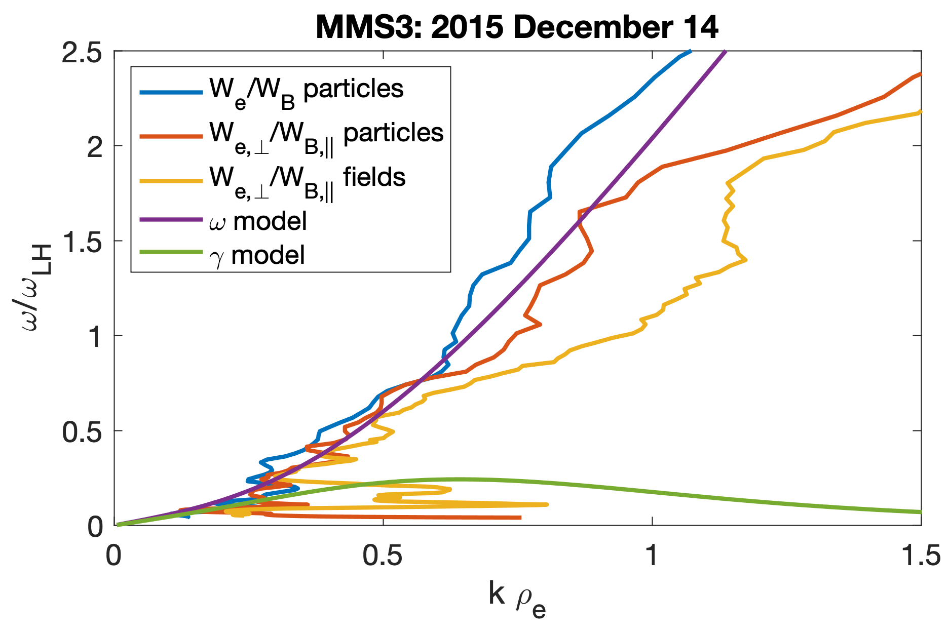
Figure 18: Lower hybrid wave dispersion relations calculated using equations (35) and (38) for the lower hybrid waves observed on 2015 December 14 from Figure 15. The blue, red, and yellow curves are the dispersion relations computed equation (35) using electron moments, equation (38) using electron moments, and equation (38) using only fields data. The purple and green lines are the modeled LHDI dispersion relation and growth rate.

Figure 18 compares the dispersion relations computed using equations (35) and (38). The blue line show the dispersion relations using equation (35) and electron moments (reproduced from Figure 15), the red line shows the dispersion relation computed from equation (38) using electron moments for $W_{e,\perp}$, and the yellow line shows the dispersion from (38) using ${\bf E}$ to estimate $W_{e,\perp}$. All three methods predict similar $k$ for $\omega/\omega_{LH}\sim 0.5$, where the electric field power peaks (Figure 15). At higher frequencies larger $k$ are calculated when only fields are used, and the smallest $k$ are predicted when equation (35) is used. For $\omega/\omega_{LH}\lesssim 0.25$, there is a large increase in $k$ when only fields are used. However, in this frequency range spatial changes due to the motion of the magnetopause with respect to spacecraft may result in field or particle powers that are not associated with waves. Overall, similar qualitative results are found for the three methods, and agree well with the model dispersion relation, and similar $k$ are found for the lower hybrid frequencies where the electric field power peaks.

References

- André (1985) André, M. (1985), Dispersion surfaces, J. Plasma. Phys., 33, 1–19, 10.1017/S0022377800002270.
- Bale et al. (2002) Bale, S. D., F. S. Mozer, and T. Phan (2002), Observation of lower hybrid drift instability in the diffusion region at a reconnecting magnetopause, Geophys. Res. Lett., 29, 2180, 10.1029/2002GL016113.
- Cairns and McMillan (2005) Cairns, I. H., and B. F. McMillan (2005), Electron acceleration by lower hybrid waves in magnetic reconnection regions, Phys. Plasmas, 12, 102,110, 10.1063/1.2080567.
- Cassak and Shay (2007) Cassak, P. A., and M. A. Shay (2007), Scaling of asymmetric magnetic reconnection: General theory and collisional simulations, Phys. Plasmas, 14, 102,114, 10.1063/1.2795630.
- Che et al. (2010) Che, H., J. F. Drake, M. Swisdak, and P. H. Yoon (2010), Electron holes and heating in the reconnection dissipation region, Geophys. Res. Lett., 37, L11,105, 10.1029/2010GL043608.
- Chen et al. (2017) Chen, L.-J., M. Hesse, S. Wang, D. Gershman, R. E. Ergun, J. Burch, N. Bessho, R. B. Torbert, B. Giles, J. Webster, C. Pollock, J. Dorelli, T. Moore, W. Paterson, B. Lavraud, R. Strangeway, C. Russell, Y. Khotyaintsev, P.-A. Lindqvist, and L. Avanov (2017), Electron diffusion region during magnetopause reconnection with an intermediate guide field: Magnetospheric multiscale observations, Journal of Geophysical Research: Space Physics, pp. n/a–n/a, 10.1002/2017JA024004.
- Chew et al. (1956) Chew, G. F., M. L. Goldberger, and F. E. Low (1956), The boltzmann equation and the one-fluid hydromagnetic equations in the absence of particle collisions, Proceedings of the Royal Society of London Series A, 236, 112–118, 10.1098/rspa.1956.0116.
- Daughton (2003) Daughton, W. (2003), Electromagnetic properties of the lower-hybrid drift instability in a thin current sheet, Phys. Plasmas, 10, 3103, 10.1063/1.1594724.
- Davidson and Gladd (1975) Davidson, R. C., and N. T. Gladd (1975), Anomalous transport properties associated with the lower-hybrid-drift instability, Phys. Fluids, 18, 1327, 10.1063/1.861021.
- Davidson et al. (1977) Davidson, R. C., N. T. Gladd, C. S. Wu, and J. D. Huba (1977), Effects of finite plasma beta on the lower-hybrid-drift instability, Phys. Fluids, 20, 301, 10.1063/1.861867.
- Divin et al. (2015) Divin, A., Y. V. Khotyaintsev, A. Vaivads, M. André, S. Markidis, and G. Lapenta (2015), Evolution of the lower hybrid drift instability at reconnection jet front, Journal of Geophysical Research (Space Physics), 120, 2675–2690, 10.1002/2014JA020503.
- Egedal et al. (2011) Egedal, J., A. Le, P. L. Pritchett, and W. Daughton (2011), Electron dynamics in two-dimensional asymmetric anti-parallel reconnection, Phys. Plasmas, 18, 102,901, 10.1063/1.3646316.
- Egedal et al. (2013) Egedal, J., A. Le, and W. Daughton (2013), A review of pressure anisotropy caused by electron trapping in collisionless plasma, and its implications for magnetic reconnection, Phys. Plasmas, 20, 061,201, 10.1063/1.4811092.
- Egedal et al. (2015) Egedal, J., W. Daughton, A. Le, and A. L. Borg (2015), Double layer electric fields aiding the production of energetic flat-top distributions and superthermal electrons within magnetic reconnection exhausts, Phys. Plasmas, 22, 101,208, 10.1063/1.4933055.
- Ergun et al. (2016) Ergun, R. E., S. Tucker, J. Westfall, K. A. Goodrich, D. M. Malaspina, D. Summers, J. Wallace, M. Karlsson, J. Mack, N. Brennan, B. Pyke, P. Withnell, R. Torbert, J. Macri, D. Rau, I. Dors, J. Needell, P.-A. Lindqvist, G. Olsson, and C. M. Cully (2016), The Axial Double Probe and Fields Signal Processing for the MMS Mission, Space Sci. Rev., 199, 167–188, 10.1007/s11214-014-0115-x.
- Ergun et al. (2017) Ergun, R. E., L.-J. Chen, F. D. Wilder, N. Ahmadi, S. Eriksson, M. E. Usanova, K. A. Goodrich, J. C. Holmes, A. P. Sturner, D. M. Malaspina, D. L. Newman, R. B. Torbert, M. R. Argall, P.-A. Lindqvist, J. L. Burch, J. M. Webster, J. F. Drake, L. Price, P. A. Cassak, M. Swisdak, M. A. Shay, D. B. Graham, R. J. Strangeway, C. T. Russell, B. L. Giles, J. C. Dorelli, D. Gershman, L. Avanov, M. Hesse, B. Lavraud, O. Le Contel, A. Retino, T. D. Phan, M. V. Goldman, J. E. Stawarz, S. J. Schwartz, J. P. Eastwood, K.-J. Hwang, R. Nakamura, and S. Wang (2017), Drift waves, intense parallel electric fields, and turbulence associated with asymmetric magnetic reconnection at the magnetopause, Geophys. Res. Lett., 44, 2978–2986, 10.1002/2016GL072493.
- Graham et al. (2014) Graham, D. B., Y. V. Khotyaintsev, A. Vaivads, M. André, and A. N. Fazakerley (2014), Electron dynamics in the diffusion region of an asymmetric magnetic reconnection, Phys. Rev. Lett., 112, 215,004, 10.1103/PhysRevLett.112.215004.
- Graham et al. (2015) Graham, D. B., Y. V. Khotyaintsev, A. Vaivads, and M. André (2015), Electrostatic solitary waves with distinct speeds associated with asymmetric reconnection, Geophys. Res. Lett., 42, 215, 10.1002/2014GL062538.
- Graham et al. (2016a) Graham, D. B., Y. V. Khotyaintsev, C. Norgren, A. Vaivads, M. André, P.-A. Lindqvist, G. T. Marklund, R. E. Ergun, W. R. Paterson, D. J. Gershman, B. L. Giles, C. J. Pollock, J. C. Dorelli, L. A. Avanov, B. Lavraud, Y. Saito, W. Magnes, C. T. Russell, R. J. Strangeway, R. B. Torbert, and J. L. Burch (2016a), Electron currents and heating in the ion diffusion region of asymmetric reconnection, Geophys. Res. Lett., 43, 4691–4700, 10.1002/2016GL068613.
- Graham et al. (2016b) Graham, D. B., Y. V. Khotyaintsev, A. Vaivads, and M. André (2016b), Electrostatic solitary waves and electrostatic waves at the magnetopause, Journal of Geophysical Research: Space Physics, 121, 3069–3092, 10.1002/2015JA021527.
- Graham et al. (2017a) Graham, D. B., Y. V. Khotyaintsev, C. Norgren, A. Vaivads, M. André, S. Toledo-Redondo, P.-A. Lindqvist, G. T. Marklund, R. E. Ergun, W. R. Paterson, D. J. Gershman, B. L. Giles, C. J. Pollock, J. C. Dorelli, L. A. Avanov, B. Lavraud, Y. Saito, W. Magnes, C. T. Russell, R. J. Strangeway, R. B. Torbert, and J. L. Burch (2017a), Lower hybrid waves in the ion diffusion and magnetospheric inflow regions, Journal of Geophysical Research: Space Physics, 10.1002/2016JA023572.
- Graham et al. (2017b) Graham, D. B., Y. V. Khotyaintsev, A. Vaivads, C. Norgren, M. André, J. M. Webster, J. L. Burch, P.-A. Lindqvist, R. E. Ergun, R. B. Torbert, W. R. Paterson, D. J. Gershman, B. L. Giles, W. Magnes, and C. T. Russell (2017b), Instability of agyrotropic electron beams near the electron diffusion region, Phys. Rev. Lett., 119, 025,101, 10.1103/PhysRevLett.119.025101.
- Hsia et al. (1979) Hsia, J. B., S. M. Chiu, M. F. Hsia, R. L. Chou, and C. S. Wu (1979), Generalized lower-hybrid-drift instability, Phys. Fluids, 22, 1737–1746, 10.1063/1.862810.
- Huba et al. (1977) Huba, J. D., N. T. Gladd, and K. Papadopoulos (1977), The lower-hybrid-drift instability as a source of anomalous resistivity for magnetic field line reconnection, Geophys. Res. Lett., 4, 125–128.
- Khotyaintsev et al. (2016) Khotyaintsev, Y. V., D. B. Graham, C. Norgren, E. Eriksson, W. Li, A. Johlander, A. Vaivads, M. André, P. L. Pritchett, A. Retino, T. D. Phan, R. E. Ergun, K. Goodrich, P.-A. Lindqvist, G. T. Marklund, O. L. Contel, F. Plaschke, W. Magnes, R. J. Strangeway, C. T. Russell, H. Vaith, M. R. Argall, C. A. Kletzing, R. Nakamura, R. B. Torbert, W. R. Paterson, D. J. Gershman, J. C. Dorelli, L. A. Avanov, B. Lavraud, Y. Saito, B. L. Giles, C. J. Pollock, D. L. Turner, J. D. Blake, J. F. Fennell, A. Jaynes, B. H. Mauk, and J. L. Burch (2016), Electron jet of asymmetric reconnection, Geophys. Res. Lett., 43, 5571–5580, 10.1002/2016GL069064.
- Krall and Liewer (1971) Krall, N. A., and P. C. Liewer (1971), Low-frequency instabilities in magnetic pulses, Phys. Rev. A, 4, 2094, 10.1103/PhysRevA.4.2094.
- Le et al. (2009) Le, A., J. Egedal, W. Daughton, W. Fox, and N. Katz (2009), Equations of state for collisionless guide-field reconnection, Phys. Rev. Lett., 102, 085,001, 10.1103/PhysRevLett.102.085001.
- Le et al. (2017) Le, A., W. Daughton, L.-J. Chen, and J. Egedal (2017), Enhanced electron mixing and heating in 3-d asymmetric reconnection at the earth’s magnetopause, Geophys. Res. Lett., 44, 2096–2104, 10.1002/2017GL072522.
- Le et al. (2018) Le, A., W. Daughton, O. Ohia, L.-J. Chen, Y.-H. Liu, S. Wang, W. D. Nystrom, and R. Bird (2018), Drift turbulence, particle transport, and anomalous dissipation at the reconnecting magnetopause, Physics of Plasmas, 25, 062,103, 10.1063/1.5027086.
- Le Contel et al. (2016) Le Contel, O., P. Leroy, A. Roux, C. Coillot, D. Alison, A. Bouabdellah, L. Mirioni, L. Meslier, A. Galic, M. C. Vassal, R. B. Torbert, J. Needell, D. Rau, I. Dors, R. E. Ergun, J. Westfall, D. Summers, J. Wallace, W. Magnes, A. Valavanoglou, G. Olsson, M. Chutter, J. Macri, S. Myers, S. Turco, J. Nolin, D. Bodet, K. Rowe, M. Tanguy, and B. de la Porte (2016), The Search-Coil Magnetometer for MMS, Space Sci. Rev., 199, 257–282, 10.1007/s11214-014-0096-9.
- Lindqvist et al. (2016) Lindqvist, P.-A., G. Olsson, R. B. Torbert, B. King, M. Granoff, D. Rau, G. Needell, S. Turco, I. Dors, P. Beckman, J. Macri, C. Frost, J. Salwen, A. Eriksson, L. Åhlén, Y. V. Khotyaintsev, J. Porter, K. Lappalainen, R. E. Ergun, W. Wermeer, and S. Tucker (2016), The Spin-Plane Double Probe Electric Field Instrument for MMS, Space Sci. Rev., 199, 137–165, 10.1007/s11214-014-0116-9.
- McBride et al. (1972) McBride, J. B., E. Ott, J. P. Boris, and J. H. Orens (1972), Theory and simulation of turbulent heating by the modified two-stream instability, Phys. Fluids, 15, 2367–2383, 10.1063/1.1693881.
- Norgren et al. (2012) Norgren, C., A. Vaivads, Y. V. Khotyaintsev, and M. Andre (2012), Lower hybrid drift waves: Space observations, Phys. Rev. Lett., 109, 055,001, 10.1103/PhysRevLett.109.055001.
- Pan et al. (2018) Pan, D.-X., Y. V. Khotyaintsev, D. B. Graham, A. Vaivads, X.-Z. Zhou, M. André, P.-A. Lindqvist, R. E. Ergun, O. Le Contel, C. T. Russell, R. B. Torbert, B. Giles, and J. L. Burch (2018), Rippled Electron-Scale Structure of a Dipolarization Front, Geophys. Res. Lett., 45, 12, 10.1029/2018GL080826.
- Pollock et al. (2016) Pollock, C., T. Moore, A. Jacques, J. Burch, U. Gliese, Y. Saito, T. Omoto, L. Avanov, A. Barrie, V. Coffey, J. Dorelli, D. Gershman, B. Giles, T. Rosnack, C. Salo, S. Yokota, M. Adrian, C. Aoustin, C. Auletti, S. Aung, V. Bigio, N. Cao, M. Chandler, D. Chornay, K. Christian, G. Clark, G. Collinson, T. Corris, A. De Los Santos, R. Devlin, T. Diaz, T. Dickerson, C. Dickson, A. Diekmann, F. Diggs, C. Duncan, A. Figueroa-Vinas, C. Firman, M. Freeman, N. Galassi, K. Garcia, G. Goodhart, D. Guererro, J. Hageman, J. Hanley, E. Hemminger, M. Holland, M. Hutchins, T. James, W. Jones, S. Kreisler, J. Kujawski, V. Lavu, J. Lobell, E. LeCompte, A. Lukemire, E. MacDonald, A. Mariano, T. Mukai, K. Narayanan, Q. Nguyan, M. Onizuka, W. Paterson, S. Persyn, B. Piepgrass, F. Cheney, A. Rager, T. Raghuram, A. Ramil, L. Reichenthal, H. Rodriguez, J. Rouzaud, A. Rucker, Y. Saito, M. Samara, J.-A. Sauvaud, D. Schuster, M. Shappirio, K. Shelton, D. Sher, D. Smith, K. Smith, S. Smith, D. Steinfeld, R. Szymkiewicz, K. Tanimoto, J. Taylor, C. Tucker, K. Tull, A. Uhl, J. Vloet, P. Walpole, S. Weidner, D. White, G. Winkert, P.-S. Yeh, and M. Zeuch (2016), Fast Plasma Investigation for Magnetospheric Multiscale, Space Sci. Rev., 199, 331–406, 10.1007/s11214-016-0245-4.
- Price et al. (2016) Price, L., M. Swisdak, J. F. Drake, P. A. Cassak, J. T. Dahlin, and R. E. Ergun (2016), The effects of turbulence on three-dimensional magnetic reconnection at the magnetopause, Geophys. Res. Lett., 43, 6020–6027, 10.1002/2016GL069578.
- Price et al. (2017) Price, L., M. Swisdak, J. F. Drake, J. L. Burch, P. A. Cassak, and R. E. Ergun (2017), Turbulence in Three-Dimensional Simulations of Magnetopause Reconnection, Journal of Geophysical Research (Space Physics), 122, 11,086–11,099, 10.1002/2017JA024227.
- Pritchett (2013) Pritchett, P. L. (2013), The influence of intense electric fields on three-dimensional asymmetric magnetic reconnection, Phys. Plasmas, 20, 061,204, 10.1063/1.4811123.
- Pritchett and Coroniti (2010) Pritchett, P. L., and F. V. Coroniti (2010), A kinetic ballooning/interchange instability in the magnetotail, Journal of Geophysical Research (Space Physics), 115, A06,301, 10.1029/2009JA014752.
- Pritchett and Mozer (2011) Pritchett, P. L., and F. S. Mozer (2011), Rippling mode in the sub solar magnetopause current layer and its influence on three-dimensional magnetic reconnection, J. Geophys. Res., 116, A04,215.
- Pritchett et al. (2012) Pritchett, P. L., F. S. Mozer, and M. Wilber (2012), Intense perpendicular electric fields associated with three-dimensional magnetic reconnection at the subsolar magnetopause, J. Geophys. Res., 117, A06,212, 10.1029/2012JA017533.
- Rager et al. (2018) Rager, A. C., J. C. Dorelli, D. J. Gershman, V. Uritsky, L. A. Avanov, R. B. Torbert, J. L. Burch, R. E. Ergun, J. Egedal, C. Schiff, J. R. Shuster, B. L. Giles, W. R. Paterson, C. J. Pollock, R. J. Strangeway, C. T. Russell, B. Lavraud, V. N. Coffey, and Y. Saito (2018), Electron crescent distributions as a manifestation of diamagnetic drift in an electron scale current sheet: Magnetospheric multiscale observations using new 7.5 ms fast plasma investigation moments, Geophysical Research Letters, pp. 578–584, 10.1002/2017GL076260.
- Russell et al. (2016) Russell, C. T., B. J. Anderson, W. Baumjohann, K. R. Bromund, D. Dearborn, D. Fischer, G. Le, H. K. Leinweber, D. Leneman, W. Magnes, J. D. Means, M. B. Moldwin, R. Nakamura, D. Pierce, F. Plaschke, K. M. Rowe, J. A. Slavin, R. J. Strangeway, R. Torbert, C. Hagen, I. Jernej, A. Valavanoglou, and I. Richter (2016), The magnetospheric multiscale magnetometers, Space Sci. Rev., 199, 189–256, 10.1007/s11214-014-0057-3.
- Silin et al. (2005) Silin, I., J. Buchner, and A. Vaivads (2005), Anomalous resistivity due to nonlinear lower-hybrid drift waves, Phys. Plasmas, 12, 062,902, 10.1063/1.1927096.
- Silveira et al. (2002) Silveira, O. J., L. F. Ziebell, R. Gaelzer, and P. H. Yoon (2002), Unified formulation for inhomogeneity-driven instabilities in the lower-hybrid range, Phys. Rev. E, 65(3), 036,407, 10.1103/PhysRevE.65.036407.
- Stix (1962) Stix, T. H. (1962), The Theory of Plasma Waves, McGraw-Hill, New York.
- Swanson (1989) Swanson, D. G. (1989), Plasma waves.
- Tanaka and Sato (1981) Tanaka, M., and T. Sato (1981), Simulations on lower hybrid drift instability and anomalous resistivity in the magnetic neutral sheet, J. Geophys. Res., 86, 5541–5552, 10.1029/JA086iA07p05541.
- Treumann et al. (1991) Treumann, R. A., J. Labelle, and R. Pottelette (1991), Plasma diffusion at the magnetopause - The case of lower hybrid drift waves, J. Geophys. Res., 96, 16,009, 10.1029/91JA01671.
- Vaivads et al. (2004) Vaivads, A., M. André, S. C. Buchert, J.-E. Wahlund, A. N. Fazakerley, and N. Cornilleau-Wehrlin (2004), Cluster observations of lower hybrid turbulence within thin layers at the magnetopause, Geophys. Res. Lett., 31, L03,804, 10.1029/2003GL018142.
- Wang et al. (2017) Wang, S., L.-J. Chen, M. Hesse, L. B. Wilson, N. Bessho, D. J. Gershman, R. E. Ergun, T. D. Phan, J. L. Burch, J. C. Dorelli, B. Giles, R. B. Torbert, C. J. Pollock, C. T. Russell, R. Strangeway, L. Avanov, B. Lavraud, and T. E. Moore (2017), Parallel electron heating in the magnetospheric inflow region, Geophys. Res. Lett., pp. 4384–4392, 10.1002/2017GL073404.
- Wu et al. (1983) Wu, C. S., D. Winske, K. Papadopoulos, Y. M. Zhou, S. T. Tsai, and S. C. Guo (1983), A kinetic cross-field streaming instability, Physics of Fluids, 26, 1259–1267, 10.1063/1.864285.