Spin functional renormalization group for quantum Heisenberg ferromagnets:
Magnetization and magnon damping in two dimensions

Abstract

We use the spin functional renormalization group recently developed by two of us [J. Krieg and P. Kopietz, Phys. Rev. B 99, 060403(R) (2019)] to calculate the magnetization $M(H,T)$ and the damping of magnons due to classical longitudinal fluctuations of quantum Heisenberg ferromagnets. In order to guarantee that for vanishing magnetic field $H\rightarrow 0$, the magnon spectrum is gapless when the spin rotational invariance is spontaneously broken, we use a Ward identity to express the magnon self-energy in terms of the magnetization. In two dimensions our approach correctly predicts the absence of long-range magnetic order for $H=0$ at finite temperature $T$. The magnon spectrum then exhibits a gap from which we obtain the transverse correlation length. We also calculate the wave-function renormalization factor of the magnons. As a mathematical by-product, we derive a recursive form of the generalized Wick theorem for spin operators in frequency space which facilitates the calculation of arbitrary time-ordered connected correlation functions of an isolated spin in a magnetic field.

I Introduction

Recently two of us have proposed a new approach to quantum spin systems based on a formally exact renormalization group equation for the generating functional of the connected spin correlation functions Krieg19 . Our method works directly with the physical spin operators, thus avoiding any representation of the spin operators in terms of canonical bosons or fermions acting on a projected Hilbert space. A similar strategy was adopted half a century ago by Vaks, Larkin, and Pikin (VLP) Vaks68 ; Vaks68b , who developed an unconventional diagrammatic approach to quantum spin systems based on a generalized Wick theorem for spin operators. A detailed description of this approach can be found in the textbook by Izyumov and Skryabin Izyumov88 . It turns out, however, that the diagrammatic structure of this approach is rather complicated, which is perhaps the reason why this method has not gained wide acceptance. As pointed out in Ref. [Krieg19, ], by combining the VLP approachVaks68 ; Vaks68b with modern functional renormalization group (FRG) methods Berges02 ; Pawlowski07 ; Kopietz10 ; Metzner12 , we can reduce the problem of calculating the spin correlation functions to the problem of solving the bosonic version of the Wetterich equation Wetterich93 with a special initial condition determined by the $SU(2)$-spin algebra. Our spin functional renormalization group (SFRG) approach is an extension of the lattice non-perturbative renormalization group approach developed by Machado and Dupuis Machado10 for classical spin models, and by Rançon and Dupuis Rancon11a ; Rancon11b ; Rancon12a ; Rancon12b ; Rancon14 for bosonic quantum lattice models. Another FRG approach to quantum spin systems is the so-called pseudofermion FRGReuther10 ; Reuther11 ; Reuther11a ; Buessen16 , which uses the representation of spin-$1/2$ operators in terms of Abrikosov pseudofermions Coleman15 to approximate the renormalization group flow of spin-$1/2$ quantum spin systems by a truncated fermionic FRG flow Kopietz01 ; Metzner12 . The pseudofermion FRG has been quite successful to map out the phase diagram of various types of frustrated magnets without long-range magnetic order.Reuther10 ; Reuther11 ; Reuther11a ; Buessen16 In contrast to the pseudofermion FRG, our SFRG can be used for arbitrary spin $S$ because it does not rely on the representation of the spin operators in terms of auxiliary degrees of freedom.

As a first application of our SFRG approach, in Ref. [Tarasevych18, ] we have shown how Anderson’s poor man’s scaling equations for the anisotropic Kondo model emerge from a simple weak coupling truncation of the SFRG flow equations for the irreducible vertices of this model. Our ultimate goal is to develop the SFRG method into a quantitative tool for studying quantum spin systems which is valid both in the magnetically ordered and the disordered phases. To realize this program, it is important to test the method for model systems where the physics is well understood and quantitatively accurate results can be obtained by means of other methods. Here we will use the SFRG to study the spin-$S$ ferromagnetic quantum Heisenberg model in two dimensions. At any finite temperature $T>0$ the magnetization $M(H,T>0)$ of this model is rigorously known Mermin66 to vanish when the external magnetic field $H$ approaches zero, so that conventional spin-wave theory breaks down for $H\rightarrow 0$. If we nevertheless try to calculate the magnetization for $H=0$ perturbatively, we encounter infrared divergencies signalling the breakdown of perturbation theory Hofmann02 .

Theoretical investigations of quantum Heisenberg ferromagnets in two dimensions have a long history. In the 1980s several approximate analytical methods have been developed to calculate the thermodynamics and the spectrum of renormalized magnons at finite temperature. For example, in Takahashi’s modified spin-wave theory Takahashi86 ; Takahashi87 the vanishing of the magnetization for $H=0$ is enforced by adding an effective chemical potential to the magnon energies which regularizes the infrared divergence encountered in perturbation theory. Note, however, that for finite magnetic field $H$ this strategy is not applicable because then the magnetization does not vanish. One possibility to generalize Takahashi’s modified spin-wave theory for finite magnetic field is to consider the spin-wave expansion of the Gibbs potential for fixed magnetization Kollar03 . Another useful method is based on the representation of the spin operators in terms of Schwinger bosons Arovas88 . This representation maps the exchange interaction between spins onto a quartic boson Hamiltonian with an additional constraint on the physical Hilbert space. Often a simple mean-field treatment of the resulting effective boson problem gives already sensible results, so that Schwinger boson mean-field theory continues to be a popular analytical method for studying spin systems without long-range magnetic order. However, going beyond the mean-field approximation is rather difficult within the Schwinger boson approach Chubukov91 ; Trumper97 ; Timm98 ; Ghioldi18 . Another analytical approach to quantum ferromagnets is based on the decoupling of the equations of motion for the Green functions of the spins Tyablikov67 ; Junger04 ; Junger08 . Of course, the physical properties of quantum ferromagnets can be obtained with high accuracy numerically using Monte Carlo simulations Kopietz89 ; Kopietz89b ; Henelius00 .

In Ref. [Kopietz89, ] the correlation length and the susceptibility of a two-dimensional quantum Heisenberg ferromagnet have been calculated via a special implementation of the momentum-shell Wilsonian renormalization group (RG) technique using the Holstein-Primakoff transformation to express the spin operators in terms of bosons. At the level of a one-loop approximation the results for the correlation length and the susceptibility agree with modified spin-wave theory Takahashi86 ; Takahashi87 and Schwinger boson mean-field theory,Arovas88 but the two-loop corrections have been found to modify the one-loop results Kopietz89 . In the present work, we will show that the one-loop flow equations derived in Ref. [Kopietz89, ] can be obtained in a straightforward way within our SFRG formalism from a truncated flow equation for the magnetization. We then use the SFRG to derive an improved flow equation for the magnetization which takes into account self-energy and vertex corrections neglected in Ref. [Kopietz89, ]. Moreover, we will also calculate the damping of spin-waves due to the coupling to classical longitudinal spin fluctuations. This decay channel of magnons is neglected in conventional spin-wave theory where the longitudinal fluctuations are not treated as independent degrees of freedom.

The rest of this work is organized as follows. In Sec. II, we define a new hybrid generating functional $\Gamma_{\Lambda}[\bm{m},\phi]$ depending on the transverse magnetization $\bm{m}$ as well as on a longitudinal exchange field $\phi$ and show that this functional satisfies the Wetterich equation Wetterich93 . In Sec. III we give the general structure of the expansion of $\Gamma_{\Lambda}[\bm{m},\phi]$ in powers of the fields and explicitly write down the exact flow equations for the magnetization and the two-point vertices. Section IV is devoted to the explicit calculation of the magnetization $M(H,T)$ of a two-dimensional Heisenberg ferromagnet. We establish the relation of our SFRG approach to the momentum shell RG of Ref. [Kopietz89, ] and go beyond this work by including self-energy and vertex corrections. In Sec. V, we calculate the damping of spin waves in two-dimensional ferromagnets due to the coupling to classical longitudinal fluctuations. In Sec. VI, we summarize our main results and point out possible extensions of our method.

In four appendices, we give additional technical details. In Appendix A, we derive the relation between the connected spin correlation functions and the irreducible vertices generated by our hybrid functional $\Gamma_{\Lambda}[\bm{m},\phi]$. In Appendix B, we give the time-ordered connected spin correlation functions of a single spin in an external magnetic field with up to four spins and derive the corresponding irreducible vertices; we also present a simple recursive form of the generalized Wick theorem for spin operators in frequency space. In Appendix C, we write down equations of motion for the time-ordered connected spin correlation functions and derive a Ward identity which we use in the main text to close the flow equation for the magnetization. Finally, in Appendix D, we derive initial conditions for the irreducible vertices in tree approximation where all terms involving loop integrations over momenta are neglected.

II Exact flow equations for quantum spin systems

In this section and in the following Sec.  III, we consider a general anisotropic Heisenberg Hamiltonian of the form

$${\cal{H}}=-H\sum_{i}S^{z}_{i}+\frac{1}{2}\sum_{ij}\left[J^{\bot}_{ij}\bm{S}^{\bot}_{i}\cdot\bm{S}^{\bot}_{j}+J^{z}_{ij}{{S}}^{z}_{i}{{S}}^{z}_{j}\right],$$ (1)

where the external magnetic field $H$ is measured in units of energy, $\bm{S}^{\bot}_{i}=(S^{x}_{i},S^{y}_{i})$ is the transverse part of the spin operator $\bm{S}_{i}$, and $J^{\bot}_{ij}$ and $J^{z}_{ij}$ are transverse and longitudinal exchange couplings. In Sec. IV, we will consider isotropic ferromagnets by specifying $J^{\bot}_{ij}=J^{z}_{ij}=-V_{ij}<0$, but at this point, we work with general anisotropic exchange couplings. Following Ref. [Krieg19, ], we now modify the Hamiltonian (1) by replacing $J^{\bot}_{ij}$ and $J^{z}_{ij}$ by deformed exchange couplings depending on a continuous parameter $\Lambda$,

$$J^{\bot}_{\Lambda,ij} = J^{\bot}_{ij}+R^{\bot}_{\Lambda,ij},\;\;\;\;\;\;J^{z}_{\Lambda,ij}=J^{z}_{ij}+R^{z}_{\Lambda,ij},$$ (2)

where the regulators $R^{\bot}_{\Lambda,ij}$ and $R^{z}_{\Lambda,ij}$ should be chosen such that for some initial $\Lambda=\Lambda_{0}$ the deformed model can be solved in a controlled way, and for some final value of $\Lambda$ the regulators vanish so that we recover our original model. For example, $\Lambda$ can be a momentum scale acting as a cutoff for long-wavelength fluctuations, or simply a dimensionless parameter in the interval $[0,1]$ which multiplies the bare interaction. At this point, it is not necessary to specify the deformation scheme. Let us write the deformed Hamiltonian in the form ${\cal{H}}_{\Lambda}={\cal{H}}_{0}+{\cal{V}}_{\Lambda}$, where

$${\cal{H}}_{0} = -H\sum_{i}S^{z}_{i}$$ (3)

is the Hamiltonian of isolated spins in a constant magnetic field and

$${\cal{V}}_{\Lambda} = \frac{1}{2}\sum_{ij}\left[J^{\bot}_{\Lambda,ij}\bm{S}^{\bot}_{i}\cdot\bm{S}^{\bot}_{j}+J^{z}_{\Lambda,ij}{{S}}^{z}_{i}{{S}}^{z}_{j}\right]$$ (4)

represents the coupling between the spins. The generating functional of the deformed Euclidean time-ordered spin correlation functions can then be written as Krieg19

$${\cal{G}}_{\Lambda}[\bm{h}]=\ln{\rm Tr}\left[e^{-\beta{\cal{H}}_{0}}{\cal{T}}e^{\int_{0}^{\beta}d\tau[\sum_{i}\bm{h}_{i}(\tau)\cdot{{\bm{S}}_{i}(\tau)-{\cal{V}}_{\Lambda}(\tau)]}}\right].$$ (5)

Here $\beta$ is the inverse temperature, ${\cal{T}}$ denotes time-ordering in imaginary time, $\bm{h}_{i}(\tau)$ are fluctuating source fields, and the time dependence of all operators is in the interaction picture with respect to ${\cal{H}}_{0}$. By simply taking a derivative of both sides of Eq. (5) with respect to $\Lambda$ we can derive an exact functional flow equation for the generating functional ${\cal{G}}_{\Lambda}[\bm{h}]$. Moreover, the Legendre transform of ${\cal{G}}_{\Lambda}[\bm{h}]$ satisfies an exact functional flow equation which is formally identical to the bosonic version of the Wetterich equation Krieg19 ; Wetterich93 . A technical complication of this method is that in a scheme where initially the exchange couplings are completely switched off the Legendre transform of ${\cal{G}}_{\Lambda=0}[\bm{h}]$ does not exist Rancon14 ; Krieg19 because in this limit the longitudinal spin fluctuations do not have any dynamics. In Ref. [Krieg19, ] we have already pointed out that this problem can be avoided by working with the generating functional of the amputated connected correlation functions. Here we show how this idea is implemented in practice. Actually, because only the longitudinal fluctuations are initially static, it is convenient to introduce a hybrid functional ${\cal{F}}_{\Lambda}[\bm{h}^{\bot},s]$ which generates connected correlation functions for transverse fluctuations, but amputates the external legs associated with the longitudinal fluctuations. Formally, this functional can be defined by

$${\cal{F}}_{\Lambda}[\bm{h}^{\bot},s] = {\cal{G}}_{\Lambda}\Bigl{[}\bm{h}^{\bot}_{i},h_{i}^{z}=-\sum_{j}{J}^{z}_{\Lambda,ij}s_{j}\Bigr{]}$$ (6)

$$- \frac{1}{2}\int_{0}^{\beta}d\tau\sum_{ij}{J}^{z}_{\Lambda,ij}s_{i}(\tau)s_{j}(\tau),\hskip 19.91692pt$$

where $\bm{h}^{\bot}_{i}=(h^{x}_{i},h^{y}_{i})$ is a transverse magnetic source field, and $s_{i}(\tau)$ is a longitudinal source field which can be interpreted as a fluctuating magnetic moment in the direction of the external field. Note that a similar hybrid functional of “partially amputated connected” correlation functions has been introduced earlier in Ref. [Schuetz06, ] to derive partially bosonized FRG flow equations for interacting fermions. By expanding ${\cal{F}}_{\Lambda}[\bm{h}^{\bot},s]$ in powers of the source fields $\bm{h}^{\bot}_{i}(\tau)$ and $s_{i}(\tau)$, we obtain connected spin correlation functions with the additional property that external legs associated with longitudinal propagators are amputated Krieg19 . As a consequence, correlation functions generated by ${\cal{F}}_{\Lambda}[\bm{h}^{\bot},s]$ with longitudinal external legs involve powers of the longitudinal interaction $J^{z}_{\Lambda,ij}$ and therefore vanish for $J^{z}_{\Lambda,ij}\rightarrow 0$. For example, the longitudinal two-point function is given by

$$F_{\Lambda,ij}(\tau,\tau^{\prime})=\left.\frac{\delta^{2}{\cal{F}}_{\Lambda}[\bm{h}^{\bot}_{i}=0,s]}{\delta s_{i}(\tau)\delta s_{j}(\tau^{\prime})}\right|_{s=0}$$

$$=-\delta(\tau-\tau^{\prime})J^{z}_{\Lambda,ij}+\sum_{kl}J^{z}_{\Lambda,ik}J^{z}_{\Lambda,jl}G^{zz}_{\Lambda,kl}(\tau,\tau^{\prime}),$$ (7)

where

$$G^{zz}_{\Lambda,ij}(\tau,\tau^{\prime})\left.\frac{\delta^{2}{\cal{G}}_{\Lambda}[\bm{h}]}{\delta h^{z}_{i}(\tau)\delta h^{z}_{j}(\tau^{\prime})}\right|_{\bm{h}=0}$$ (8)

is the longitudinal part of the time-ordered two-spin correlation function. The relations between the higher order longitudinal correlation functions is for $n\geq 3$,

$$F^{z\ldots z}_{\Lambda,i_{1}\ldots i_{n}}(\tau_{1},\ldots,\tau_{n})=\frac{\delta^{n}\mathcal{F}_{\Lambda}[\bm{h}^{\bot}=0,s]}{\delta s_{i_{1}}(\tau_{1})\ldots\delta s_{i_{n}}(\tau_{n})}\Big{|}_{s=0}$$

$$=(-1)^{n}\sum_{j_{1}\ldots j_{n}}J_{\Lambda,i_{1}j_{1}}^{z}\ldots J_{\Lambda,i_{n}j_{n}}^{z}G_{\Lambda,j_{1}\ldots j_{n}}^{z\ldots z}(\tau_{1},...,\tau_{n}),\hskip 19.91692pt$$ (9)

where

$$G_{\Lambda,i_{1}\ldots i_{n}}^{z\ldots z}(\tau_{1},...,\tau_{n})=\frac{\delta^{n}\mathcal{G}_{\Lambda}[\bm{h}]}{\delta h^{z}_{i_{1}}(\tau_{1})\ldots\delta h^{z}_{i_{n}}(\tau_{n})}\Big{|}_{\bm{h}=0}.$$ (10)

If we work with a deformation scheme where initially all exchange couplings vanish, all correlation functions generated by ${\cal{F}}_{\Lambda}[\bm{h}^{\bot},s]$ involving longitudinal legs also vanish at the initial scale, so that at the first sight this functional does not give rise to a convenient initial condition for this cutoff scheme. However, the Legendre transform of the functional ${\cal{F}}_{\Lambda}[\bm{h}^{\bot},s]$ has a well-defined limit for vanishing exchange couplings because the externals legs associated with the longitudinal propagators are removed in the Legendre transform. As usual, we subtract the regulator terms from the Legendre transform and define the generating functional of the irreducible vertices as follows,

$$\Gamma_{\Lambda}[\bm{m},\phi]=\int_{0}^{\beta}d\tau\sum_{i}(\bm{m}_{i}\cdot\bm{h}^{\bot}_{i}+\phi_{i}s_{i})-{\cal{F}}_{\Lambda}[\bm{h}^{\bot},s]$$

$$-\frac{1}{2}\int_{0}^{\beta}d\tau\sum_{ij}\left({R}^{\bot}_{\Lambda,ij}{\bm{m}}_{i}\cdot{\bm{m}}_{j}+{R}^{\phi}_{\Lambda,ij}\phi_{i}\phi_{j}\right),\hskip 19.91692pt$$ (11)

where the transverse and longitudinal regulators are given by

$${R}^{\bot}_{\Lambda,ij} = {J}^{\bot}_{\Lambda,ij}-{J}^{\bot}_{ij},$$ (12)

$${R}^{\phi}_{\Lambda,ij} = -[{\mathbbm{J}}^{z}_{\Lambda}]^{-1}_{ij}+[{\mathbbm{J}}^{z}]^{-1}_{ij}.$$ (13)

Here ${\mathbbm{J}}^{z}_{\Lambda}$ is a matrix on the spatial labels with matrix elements $[{\mathbbm{J}}^{z}_{\Lambda}]_{ij}={J}_{\Lambda,ij}^{z}$. Note that on the right-hand side of Eq. (11) the sources $\bm{h}_{i}^{\bot}(\tau)$ and $s_{i}(\tau)$ should be expressed in terms of the transverse magnetization $\bm{m}_{i}(\tau)$ and the longitudinal exchange field $\phi_{i}(\tau)$ by inverting the relations

$$\bm{m}_{i}(\tau) = \frac{\delta{\cal{F}}_{\Lambda}[\bm{h}^{\bot},s]}{\delta\bm{h}^{\bot}_{i}(\tau)}=\langle{\cal{T}}\bm{S}^{\bot}_{j}(\tau)\rangle,$$ (14)

$$\phi_{i}(\tau) = \frac{\delta{\cal{F}}_{\Lambda}[\bm{h}^{\bot},s]}{\delta s_{i}(\tau)}$$ (15)

$$= -\sum_{j}{J}^{z}_{\Lambda,ij}\left[s_{j}(\tau)+\langle{\cal{T}}S^{z}_{j}(\tau)\rangle\right],$$

where the expectation values $\langle{\cal{T}}\bm{S}^{\bot}_{j}(\tau)\rangle$ and $\langle{\cal{T}}S^{z}_{j}(\tau)\rangle$ should be evaluated for finite sources $\bm{h}^{\bot}_{i}(\tau)$ and $s_{i}(\tau)$. From the last line in Eq. (15), we see that for $s_{i}(\tau)=0$ the field $\phi_{i}(\tau)$ can be identified with the exchange correction to the external magnetic field. Obviously, if we use Eq. (11) to express $s_{i}(\tau)$ as a functional of $\phi_{i}(\tau)$ we obtain a factor of $[{\mathbbm{J}}^{z}_{\Lambda}]^{-1}_{ij}$ which cancels the factors of $J^{z}_{\Lambda,ij}$ in the expansion of the functional ${\cal{F}}_{\Lambda}[\bm{h}^{\bot},s]$ in powers of the longitudinal sources $s_{i}(\tau)$. The irreducible vertices generated by $\Gamma_{\Lambda}[\bm{m},\phi]$ are therefore well-defined even if we use a deformation scheme where initially all exchange couplings vanish. Another way to see this is to explicitly express the vertices generated by $\Gamma_{\Lambda}[\bm{m},\phi]$ in terms of the connected spin correlation functions, see Appendix A.

It is now straightforward to derive formally exact FRG flow equations of the two functionals ${\cal{F}}_{\Lambda}[\bm{h}^{\bot},s]$ and $\Gamma_{\Lambda}[\bm{m},\phi]$. Following the procedure outlined in Ref. [Krieg19, ], we find that the functional ${\cal{F}}_{\Lambda}[\bm{h}^{\bot},s]$ satisfies the flow equation

$$\partial_{\Lambda}{\cal{F}}_{\Lambda}[\bm{h}^{\bot},s]=-\frac{1}{2}\int_{0}^{\beta}d\tau\sum_{ij}(\partial_{\Lambda}{J}^{\bot}_{\Lambda,ij})\sum_{\alpha=x,y}\Biggl{[}\frac{\delta^{2}{\cal{F}}_{\Lambda}[\bm{h}^{\bot},s]}{\delta h_{i}^{\alpha}(\tau)\delta h_{j}^{\alpha}(\tau)}+\frac{\delta{\cal{F}}_{\Lambda}[\bm{h}^{\bot},s]}{\delta h_{i}^{\alpha}(\tau)}\frac{\delta{\cal{F}}_{\Lambda}[\bm{h}^{\bot},s]}{\delta h_{j}^{\alpha}(\tau)}\Biggr{]}$$

$$+\frac{1}{2}\int_{0}^{\beta}d\tau\sum_{ij}\left(\partial_{\Lambda}[{{\mathbbm{J}}}^{z}_{\Lambda}]_{ij}^{-1}\right)\Biggl{[}\frac{\delta^{2}{\cal{F}}_{\Lambda}[\bm{h}^{\bot},s]}{\delta s_{i}(\tau)\delta s_{j}(\tau)}+\frac{\delta{\cal{F}}_{\Lambda}[\bm{h}^{\bot},s]}{\delta s_{i}(\tau)}\frac{\delta{\cal{F}}_{\Lambda}[\bm{h}^{\bot},s]}{\delta s_{j}(\tau)}\Biggr{]}+\frac{1}{2}{\rm Tr}\left[{\mathbf{J}}^{z}_{\Lambda}\partial_{\Lambda}({{\mathbf{J}}}^{z}_{\Lambda})^{-1}\right].$$ (16)

Here ${\mathbf{J}}^{z}_{\Lambda}$ is a matrix in all labels (spin component, lattice site, imaginary time) with matrix elements defined by

$${[}\mathbf{{J}}^{z}_{\Lambda}]^{\alpha\alpha^{\prime}}_{i\tau,j\tau^{\prime}} = \delta(\tau-\tau^{\prime})\delta_{\alpha z}\delta_{\alpha^{\prime}z}[{\mathbbm{J}}^{z}_{\Lambda}]_{ij}=\delta(\tau-\tau^{\prime})\delta_{\alpha z}\delta_{\alpha^{\prime}z}{J}^{z}_{\Lambda,ij}.$$ (17)

With this notation the trace in the last term of Eq. (16) is over all labels; the formally divergent $\delta$-function $\delta(\tau=0)$ hidden in the last term of Eq. (16) cancels when we combine this term with a similar contribution from the second term. Differentiating both sides of Eq. (11) with respect to the deformation parameter $\Lambda$ and using Eq. (16), we obtain

$$\partial_{\Lambda}\Gamma_{\Lambda}[\bm{m},\phi]=\frac{1}{2}\int_{0}^{\beta}d\tau\sum_{ij}\biggl{[}\sum_{\alpha=x,y}\frac{\delta^{2}{\cal{F}}_{\Lambda}[\bm{h}^{\bot},s]}{\delta h_{i}^{\alpha}(\tau)\delta h_{j}^{\alpha}(\tau)}\partial_{\Lambda}R^{\bot}_{\Lambda,ij}+\frac{\delta^{2}{\cal{F}}_{\Lambda}[\bm{h}^{\bot},s]}{\delta s_{i}(\tau)\delta s_{j}(\tau)}\partial_{\Lambda}R^{\phi}_{\Lambda,ij}\biggr{]}-\frac{1}{2}{\rm Tr}\left[{\mathbf{J}}^{z}_{\Lambda}\partial_{\Lambda}({{\mathbf{J}}}^{z}_{\Lambda})^{-1}\right].$$ (18)

Note that the quadratic subtractions in Eq. (11) eliminate the terms on the right-hand side of the flow equation (16) corresponding to diagrams which are reducible with respect to cutting either a transverse propagator line or a longitudinal interaction line. Finally, we express the second derivatives on the right-hand side of Eq. (18) in terms of the matrix $\mathbf{\Gamma}^{\prime\prime}_{\Lambda}[\bm{m},\phi]$ of second functional derivatives of $\Gamma_{\Lambda}[\bm{m},\phi]$ and obtain an exact functional flow equation for our quantum spin system which formally resembles the Wetterich equation Wetterich93 ,

$$\partial_{\Lambda}\Gamma_{\Lambda}[\bm{m},\phi]$$

$$=\frac{1}{2}{\rm Tr}\left\{\left[\left(\mathbf{\Gamma}^{\prime\prime}_{\Lambda}[\bm{m},\phi]+\mathbf{R}_{\Lambda}\right)^{-1}+{\mathbf{{J}}}_{\Lambda}^{z}\right]\partial_{\Lambda}\mathbf{R}_{\Lambda}\right\}.\hskip 19.91692pt$$ (19)

Here the matrix elements of $\mathbf{\Gamma}^{\prime\prime}_{\Lambda}[\bm{m},\phi]$ are given by

$$\left(\mathbf{\Gamma}^{\prime\prime}_{\Lambda}[\bm{m},\phi]\right)_{i\tau\alpha,j\tau^{\prime}\alpha^{\prime}}=\frac{\delta^{2}\Gamma_{\Lambda}[\bm{m},\phi]}{\delta\Phi^{\alpha}_{i}(\tau)\delta\Phi^{\alpha^{\prime}}_{j}(\tau^{\prime})},$$ (20)

where we have combined the two components of $\bm{m}_{i}(\tau)$ together with $\phi_{i}(\tau)$ into a three-component field

$$\left(\begin{array}[]{c}\Phi_{i}^{x}\\ \Phi_{i}^{y}\\ \Phi_{i}^{z}\end{array}\right)=\left(\begin{array}[]{c}{m}^{x}_{i}\\ m^{y}_{i}\\ \phi_{i}\end{array}\right),$$ (21)

and $\mathbf{R}_{\Lambda}$ is diagonal in the field labels with matrix elements

$${[}\mathbf{R}_{\Lambda}]^{xx}_{i\tau,j\tau^{\prime}} = {[}\mathbf{R}_{\Lambda}]^{yy}_{i\tau,j\tau^{\prime}}=\delta(\tau-\tau^{\prime}){R}^{\bot}_{\Lambda,ij},$$ (22)

$${[}\mathbf{R}_{\Lambda}]^{zz}_{i\tau,j\tau^{\prime}} = \delta(\tau-\tau^{\prime})R^{\phi}_{\Lambda,ij}.$$ (23)

For finite external field $H$ or in the presence of a finite spontaneous magnetization the expectation value $\langle S^{z}_{i}(\tau)\rangle$ is finite even for vanishing sources $s_{i}(\tau)$. Then the functional $\Gamma_{\Lambda}[\bm{m}=0,\phi]$ is extremal for a finite value $\phi_{\Lambda}$ of the exchange field,

$$\left.\frac{\delta\Gamma_{\Lambda}[\bm{m}=0,\phi]}{\delta\phi_{i}(\tau)}\right|_{\phi={\phi}_{\Lambda}}=0,$$ (24)

where ${\phi}_{\Lambda}$ can be identified with the scale-dependent renormalization of the external magnetic field due to the exchange interaction. It is then convenient to shift the field $\phi_{i}(\tau)={\phi}_{\Lambda}+\varphi_{i}(\tau)$ and consider the flow of

$$\tilde{\Gamma}_{\Lambda}[\bm{m},\varphi]=\Gamma_{\Lambda}[\bm{m},{\phi}_{\Lambda}+\varphi],$$ (25)

which is given by

$$\partial_{\Lambda}\tilde{\Gamma}_{\Lambda}[\bm{m},\varphi] = \left.\partial_{\Lambda}\Gamma_{\Lambda}[\bm{m},\phi]\right|_{\phi\rightarrow{\phi}_{\Lambda}+\varphi}$$ (26)

$$+ \int_{0}^{\beta}d\tau\sum_{i}\frac{\delta\tilde{\Gamma}_{\Lambda}[\bm{m},\varphi]}{\delta{\varphi}_{i}(\tau)}\partial_{\Lambda}{\phi}_{\Lambda}$$

$$=\frac{1}{2}{\rm Tr}\left\{\left[\left(\mathbf{\tilde{\Gamma}}^{\prime\prime}_{\Lambda}[\bm{m},\varphi]+\mathbf{R}_{\Lambda}\right)^{-1}+{\mathbf{J}}_{\Lambda}^{z}\right]\partial_{\Lambda}\mathbf{R}_{\Lambda}\right\}$$

$$+ \int_{0}^{\beta}d\tau\sum_{i}\frac{\delta\tilde{\Gamma}_{\Lambda}[\bm{m},\varphi]}{\delta{\varphi}_{i}(\tau)}\partial_{\Lambda}{\phi}_{\Lambda}.$$

III Vertex expansion

III.1 Exact flow equations

To construct an approximate solution of the exact flow equation (26), we expand the functional $\tilde{\Gamma}_{\Lambda}[\bm{m},\varphi]$ in powers of the transverse magnetization $\bm{m}_{i}(\tau)$ and the fluctuation $\varphi_{i}(\tau)$ of the longitudinal exchange field. Then we obtain an infinite hierarchy of flow equations for the irreducible vertices generated by $\tilde{\Gamma}_{\Lambda}[\bm{m},\varphi]$. It is convenient to formulate the expansion in momentum-frequency space. Introducing a collective label $K=(\bm{k},i\omega)$ for momentum $\bm{k}$ and Matsubara frequency $i\omega$, the Fourier expansion of the fields can be written as

$$\bm{m}_{i}(\tau) = \int_{K}e^{i(\bm{k}\cdot\bm{r}_{i}-\omega\tau)}\bm{m}_{K},$$ (27a)

$${\varphi}_{i}(\tau) = \int_{K}e^{i(\bm{k}\cdot\bm{r}_{i}-\omega\tau)}{\varphi}_{K},$$ (27b)

where $\int_{K}=(\beta N)^{-1}\sum_{\bm{k},\omega}$. In terms of the spherical components of the transverse magnetization,

$$m_{K}^{+}=\frac{m^{x}_{K}+im^{y}_{K}}{\sqrt{2}},\;\;\;m_{K}^{-}=\frac{m^{x}_{K}-im^{y}_{K}}{\sqrt{2}}=(m_{-K}^{+})^{\ast},$$ (28)

the vertex expansion of $\tilde{\Gamma}_{\Lambda}[\bm{m},\varphi]$ up to fourth order in the fields is of the form

$$\tilde{\Gamma}_{\Lambda}[\bm{m},\varphi] = \beta Nf_{\Lambda}+\int_{K}\Gamma^{+-}_{\Lambda}(K)m^{-}_{-K}m^{+}_{K}+\frac{1}{2!}\int_{K}\Gamma^{zz}_{\Lambda}(K)\varphi_{-K}\varphi_{K}$$ (29)

$$+ \int_{K_{1}}\int_{K_{2}}\int_{K_{3}}\delta(K_{1}+K_{2}+K_{3})\Gamma^{+-z}_{\Lambda}(K_{1},K_{2},K_{3})m^{-}_{K_{1}}m^{+}_{K_{2}}\varphi_{K_{3}}$$

$$+ \frac{1}{3!}\int_{K_{1}}\int_{K_{2}}\int_{K_{3}}\delta(K_{1}+K_{2}+K_{3})\Gamma^{zzz}_{\Lambda}(K_{1},K_{2},K_{3})\varphi_{K_{1}}\varphi_{K_{2}}\varphi_{K_{3}}$$

$$+ \int_{K_{1}}\int_{K_{2}}\int_{K_{3}}\int_{K_{4}}\delta(K_{1}+K_{2}+K_{3}+K_{4})\biggl{\{}\frac{1}{(2!)^{2}}\Gamma^{++--}_{\Lambda}(K_{1},K_{2},K_{3},K_{4})m^{-}_{K_{1}}m^{-}_{K_{2}}m^{+}_{K_{3}}m^{+}_{K_{4}}$$

$$+\frac{1}{2!}\Gamma^{+-zz}_{\Lambda}(K_{1},K_{2},K_{3},K_{4})m^{-}_{K_{1}}{m}^{+}_{K_{2}}\varphi_{K_{3}}\varphi_{K_{4}}+\frac{1}{4!}\Gamma^{zzzz}_{\Lambda}(K_{1},K_{2},K_{3},K_{4})\varphi_{K_{1}}\varphi_{K_{2}}\varphi_{K_{3}}\varphi_{K_{4}}\biggr{\}}+\ldots\;,\hskip 19.91692pt$$

where $\delta(K)=\beta N\delta_{\bm{k},0}\delta_{\omega,0}$ and we have omitted vertices with five and more external legs. The superscripts attached to the vertices refer to the field types of the associated external legs. The fact that in the expansion (29) the field $m^{-}_{K}$ is associated with the superscript ⁺ in $\Gamma_{\Lambda}^{\cdots+\cdots}(\cdots K\cdots)$ is related to the fact that $m^{-}_{K}$ is generated by differentiating ${\cal{G}}_{\Lambda}[\bm{h}]$ with respect to $h^{+}_{K}$, and $m^{+}_{K}$ can be obtained by differentiating ${\cal{G}}_{\Lambda}[\bm{h}]$ with respect to $h^{-}_{K}$ (note the alternating superscripts). The relation between the time-ordered spin correlation functions and the irreducible vertices defined via the expansion (29) is explicitly constructed in Appendix A for vertices with up to four external legs.

The exact flow equations for the vertices can be obtained from the functional flow equation (26) by expanding both sides in powers of the fields and comparing coefficients of a given power after proper symmetrization Kopietz10 . To write down the flow equations, we need the regularized transverse and longitudinal propagators

$$G_{\Lambda}(K) = \frac{1}{\Gamma^{+-}_{\Lambda}(K)+R^{\bot}_{\Lambda}(\bm{k})},$$ (30)

$$F_{\Lambda}(K) = \frac{1}{\Gamma^{zz}_{\Lambda}(K)+R^{\phi}_{\Lambda}(\bm{k})},$$ (31)

and the corresponding single-scale propagators

$$\dot{G}_{\Lambda}(K) = -[G_{\Lambda}(K)]^{2}\partial_{\Lambda}R_{\Lambda}^{\bot}(\bm{k}),$$ (32)

$$\dot{F}_{\Lambda}(K) = -[F_{\Lambda}(K)]^{2}\partial_{\Lambda}R_{\Lambda}^{\phi}(\bm{k}).$$ (33)

Here the regulator in momentum space are given by

$$R^{\bot}_{\Lambda}(\bm{k}) =J^{\bot}_{\Lambda}(\bm{k})-J^{\bot}(\bm{k}),$$ (34)

$$R^{\phi}_{\Lambda}(\bm{k}) =\frac{1}{J^{z}(\bm{k})}-\frac{1}{J^{z}_{\Lambda}(\bm{k})},$$ (35)

where we have used the discrete translational invariance of the lattice to expand the exchange couplings in momentum space,

$$J^{\bot}_{\Lambda,ij} = \frac{1}{N}\sum_{\bm{k}}e^{i\bm{k}\cdot(\bm{r}_{i}-\bm{r}_{j})}J^{\bot}_{\Lambda}({\bm{k}}),$$ (36)

$$J^{z}_{\Lambda,ij} = \frac{1}{N}\sum_{\bm{k}}e^{i\bm{k}\cdot(\bm{r}_{i}-\bm{r}_{j})}J^{z}_{\Lambda}({\bm{k}}).$$ (37)

With this notation the flow equation for the constant $f_{\Lambda}$ in Eq. (29), which can be identified with the free energy per lattice site, can be written as

$$\partial_{\Lambda}f_{\Lambda}=\int_{K} \Big{[}G_{\Lambda}(K)\partial_{\Lambda}{R}^{\bot}_{\Lambda}(\bm{k})$$

$$+\frac{1}{2}\left[F_{\Lambda}(K)+J_{\Lambda}^{z}(\bm{k})\right]\partial_{\Lambda}{R}^{\phi}_{\Lambda}(\bm{k})\Big{]}.$$ (38)

Recall that according to Eq. (7) the longitudinal propagator $F_{\Lambda}(K)$ is related to the longitudinal two-spin correlation function $G^{zz}_{\Lambda}(K)$ via

$$F_{\Lambda}(K)=-J^{z}_{\Lambda}(\bm{k})+[J^{z}_{\Lambda}(\bm{k})]^{2}G^{zz}_{\Lambda}(K),$$ (39)

so that the flow equation (38) can alternatively be written as

$$\partial_{\Lambda}f_{\Lambda}=\int_{K}\left[\dot{J}^{\bot}_{\Lambda}(\bm{k})G_{\Lambda}(K)+\frac{1}{2}\dot{J}^{z}_{\Lambda}(\bm{k})G^{zz}_{\Lambda}(K)\right],$$ (40)

where $\dot{J}^{\bot}_{\Lambda}(\bm{k})=\partial_{\Lambda}{J}^{\bot}_{\Lambda}(\bm{k})$ and $\dot{J}^{z}_{\Lambda}(\bm{k})=\partial_{\Lambda}{J}^{z}_{\Lambda}(\bm{k})$. Next, consider the flow equation for the exchange field $\phi_{\Lambda}$, which can be obtained from the condition that the expansion of the generating functional $\tilde{\Gamma}_{\Lambda}[\bm{m},\varphi]$ does not have a term linear in the fluctuation $\varphi$ (see Refs. [Schuetz06, ; Kopietz10, ]). This is guaranteed if $\phi_{\Lambda}$ flows according to

$${\Gamma}^{zz}_{\Lambda}(0)\partial_{\Lambda}{\phi}_{\Lambda} = -\int_{K}\dot{G}_{\Lambda}(K){\Gamma}_{\Lambda}^{+-z}(-K,K,0)$$ (41)

$$- \frac{1}{2}\int_{K}\dot{F}_{\Lambda}(K){\Gamma}_{\Lambda}^{zzz}(-K,K,0).\hskip 19.91692pt$$

Finally, let us also write down the exact flow equations for the transverse and longitudinal two-point vertices,

$$\partial_{\Lambda}\Gamma^{+-}_{\Lambda}(K) = {\Gamma}^{+-z}_{\Lambda}(-K,K,0)\partial_{\Lambda}\phi_{\Lambda}+\int_{Q}\dot{G}_{\Lambda}(Q){\Gamma}^{++--}_{\Lambda}(-K,-Q,Q,K)+\frac{1}{2}\int_{Q}\dot{F}_{\Lambda}(Q){\Gamma}^{+-zz}_{\Lambda}(-K,K,-Q,Q)$$ (42)

$$- \int_{Q}[\dot{G}_{\Lambda}(Q)F_{\Lambda}(Q-K)+{G}_{\Lambda}(Q)\dot{F}_{\Lambda}(Q-K)]{\Gamma}^{+-z}_{\Lambda}(-K,Q,K-Q){\Gamma}^{+-z}_{\Lambda}(-Q,K,Q-K),$$

$$\partial_{\Lambda}\Gamma^{zz}_{\Lambda}(K) = {\Gamma}^{zzz}_{\Lambda}(-K,K,0)\partial_{\Lambda}\phi_{\Lambda}+\int_{Q}\dot{G}_{\Lambda}(Q){\Gamma}^{+-zz}_{\Lambda}(-Q,Q,-K,K)+\frac{1}{2}\int_{Q}\dot{F}_{\Lambda}(Q){\Gamma}^{zzzz}_{\Lambda}(-Q,Q,-K,K)$$ (43)

$$- \int_{Q}[\dot{G}_{\Lambda}(Q)G_{\Lambda}(Q-K)+G_{\Lambda}(Q)\dot{G}_{\Lambda}(Q-K)]{\Gamma}^{+-z}_{\Lambda}(-Q,Q-K,K){\Gamma}^{+-z}_{\Lambda}(K-Q,Q,-K)$$

$$- \frac{1}{2}\int_{Q}[\dot{F}_{\Lambda}(Q)F_{\Lambda}(Q-K)+{F}_{\Lambda}(Q)\dot{F}_{\Lambda}(Q-K)]{\Gamma}^{zzz}_{\Lambda}(-Q,Q-K,K){\Gamma}^{zzz}_{\Lambda}(K-Q,Q,-K).$$

Graphical representations of the exact flow equations (41)–(43) are shown in Fig. 1.

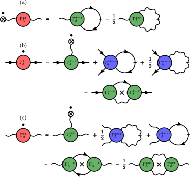
Figure 1: Graphical representation of the exact FRG flow equations (41), (42) and (43) for the exchange field and the two-point vertices. (a) Flow equation for the exchange field $\phi_{\Lambda}$; the dotted cross represents the scale derivative $\partial_{\Lambda}\phi_{\Lambda}$. The dot above the circle represents the derivative $\partial_{\Lambda}$ with respect to the deformation parameter. (b) Flow equation for the transverse two-point vertex $\Gamma^{+-}_{\Lambda}(K)$. (c) Flow equation for the longitudinal two-point vertex $\Gamma^{zz}_{\Lambda}(K)$. We use the same color coding as in Ref. [Kopietz10, ]: two-point vertices are red, three-point vertices are green, and four-point vertices are blue. Outgoing arrows represent the spherical component $m^{-}_{-K}$ of the transverse magnetization field, while incoming arrows represent the conjugate field $m^{+}_{K}$. Wavy lines are associated with the fluctuating part $\varphi$ of the longitudinal exchange field. Solid arrows and wavy lines represent transverse and longitudinal propagators, while lines with an extra slash represent the corresponding single-scale propagators. A diagram with a cross inside a loop represents the sum of two similar diagrams where each of the propagators forming the loop is successively replaced by the corresponding single-scale propagator (product rule).

Following VLP Vaks68 , it is convenient to parametrize the longitudinal spin correlation function $G^{zz}_{\Lambda}(K)$ in terms of the interaction-irreducible polarization $\Pi_{\Lambda}(K)$ by setting

$$G^{zz}_{\Lambda}(K)=\frac{\Pi_{\Lambda}(K)}{1+J^{z}_{\Lambda}(\bm{k})\Pi_{\Lambda}(K)}.$$ (44)

Using the relation (39) this implies that the longitudinal two-point function $F_{\Lambda}(K)$ generated by our functional ${\cal{F}}_{\Lambda}[\bm{h}_{\bot},s]$ can be written as

$$F_{\Lambda}(K)=-\frac{J_{\Lambda}^{z}(\bm{k})}{1+J^{z}_{\Lambda}(\bm{k})\Pi_{\Lambda}(K)}.$$ (45)

Hence, the longitudinal propagator $F_{\Lambda}(K)$ can be identified with an effective screened interaction between longitudinal spin fluctuations. Finally, using Eq. (31) to express $F_{\Lambda}(K)$ in terms of the longitudinal two-point vertex $\Gamma^{zz}_{\Lambda}(K)$ which is generated by our hybrid functional $\tilde{\Gamma}_{\Lambda}[\bm{m},\varphi]$ defined via Eqs. (11) and (25), we obtain

$$\Gamma^{zz}_{\Lambda}(K)=-\frac{1}{J^{z}(\bm{k})}-\Pi_{\Lambda}(K).$$ (46)

We conclude that, up to a minus sign, the right-hand side of the flow equation (43) for $\Gamma^{zz}_{\Lambda}(K)$ can be identified with the flow equation for the irreducible longitudinal polarization $\Pi_{\Lambda}(K)$ defined via Eq. (44).

III.2 Deformation scheme: switching off the transverse interaction

Let us now specify our deformation scheme. In general, the deformed exchange interactions $J_{\Lambda_{0},ij}^{\bot}$ and $J^{z}_{\Lambda_{0},ij}$ at the initial value $\Lambda=\Lambda_{0}$ of the deformation parameter should be chosen such that the correlation functions of the deformed model can be calculated in a controlled way.Krieg19 The simplest possibility is to completely switch off the deformed exchange couplings, $J_{\Lambda_{0},ij}^{\bot}=J^{z}_{\Lambda_{0},ij}=0$, so that the initial system consists of non-interacting spins subject to an external magnetic field. Note, however, that even in this case the time-ordered spin correlation functions and the corresponding irreducible vertex functions are rather complicated and reflect the non-trivial on-site spin correlations between different spin components implied by the $SU(2)$-spin algebra. In Appendix B we explicitly derive the corresponding initial values for the correlation functions and the vertices with up to four external legs.

In order to establish the relation of our SFRG approach and the previous momentum-shell RG calculation for quantum Heisenberg ferromagnets Kopietz89 , we choose in this work a different deformation scheme, where only the transverse interaction is initially switched off while the longitudinal interaction is not deformed at all,

$$J^{z}_{\Lambda}(\bm{k})=J^{z}(\bm{k}).$$ (47)

For our purpose it is sufficient to regularize the long-wavelength modes of the transverse interaction via a sharp cutoff,

$$J^{\bot}_{\Lambda}(\bm{k}) = \Theta(k-\Lambda)J^{\bot}(\bm{k}),$$ (48)

which amounts to the following choice of the transverse regulator:

$$R^{\bot}_{\Lambda}(\bm{k})=J^{\bot}_{\Lambda}(\bm{k})-J^{\bot}(\bm{k})=-\Theta(\Lambda-k)J^{\bot}(\bm{k}).$$ (49)

The initial value $\Lambda_{0}$ of the deformation parameter $\Lambda$ (which has units of momentum) should be chosen of the order of the inverse lattice spacing. Since $\partial_{\Lambda}J^{z}_{\Lambda}(\bm{k})=0$ in this cutoff scheme, all terms involving the longitudinal single-scale propagator $\dot{F}_{\Lambda}(K)$ in the flow equations (41–43) shown graphically in Fig. 1 can be omitted. Our deformed model at the initial scale $\Lambda=\Lambda_{0}$ is then an Ising model, which is still nontrivial.

III.3 Initial conditions

For the deformation scheme discussed above, the initial conditions for the SFRG flow are determined by the magnetization and the correlation functions of a spin S Ising model, which cannot be calculated exactly. However, in this work we are not interested in the critical regime of the Ising model, but we focus on the low-temperature regime $T\ll|J^{z}(0)|$ where a perturbative calculation of the correlation functions is possible. In order to calculate the initial conditions in a controlled way, we follow VLP and assume that the range $r_{0}$ of the exchange interaction is large compared with the lattice spacing. In this case, momentum integrals are controlled by the small parameter $1/r_{0}$, and the initial values of the correlation functions can be calculated by solving the corresponding hierarchy of equations of motion perturbatively in powers of loop integrations, see Appendix C. To leading order, i.e., in the so called tree approximation, one may simply neglect all loops. As discussed in Appendix D, then the infinite hierarchy of equations of motion decouples. The resulting initial magnetization $M_{0}=\langle S_{i}^{z}\rangle$ is given by the self-consistent mean-field approximation, obtained from the solution of

$$M_{0}=b\left(\beta\left(H+\phi_{0}\right)\right),$$ (50)

where

$$\phi_{0}=-J^{z}(0)M_{0}$$ (51)

is the initial value of the exchange field introduced in Eq. (24) and

$$b(y)=\bigl{(}S+\frac{1}{2}\bigr{)}\coth\left[\bigl{(}S+\frac{1}{2}\bigr{)}y\right]-\frac{1}{2}\coth\left[\frac{y}{2}\right]$$ (52)

is the spin-$S$ Brillouin function. The transverse two-spin correlation function is then simply given by

$$G_{0}(K) = \frac{M_{0}}{H+\phi_{0}-i\omega},$$ (53)

while the longitudinal two-spin correlation function is

$$G^{zz}_{0}(K) = \frac{\beta\delta_{\omega,0}b^{\prime}(\beta(H+\phi_{0}))}{1+J^{z}(\bm{k})\beta\delta_{\omega,0}b^{\prime}(\beta(H+\phi_{0}))}.$$ (54)

Here $b^{\prime}(y)$ is the derivative of the Brillouin function. Using Eq. (30) we find that in this case the initial value of the transverse two-point vertex is

$$\Gamma^{+-}_{0}(K) = J^{\bot}(\bm{k})+\frac{H+\phi_{0}-i\omega}{M_{0}}$$ (55)

$$= \frac{H+M_{0}[J^{\bot}(\bm{k})-J^{z}(0)]-i\omega}{M_{0}},$$

while from Eq. (44) we conclude that the intial value for the polarization is

$$\Pi_{0}(K)=\beta\delta_{\omega,0}b^{\prime}(\beta(H+\phi_{0})),$$ (56)

which according to Eq. (46) implies for the initial value of the longitudinal two-point vertex,

$$\Gamma^{zz}_{0}(K) = -\frac{1}{J^{z}(\bm{k})}-\beta\delta_{\omega,0}b^{\prime}(\beta(H+\phi_{0})),$$ (57)

The initial values of the higher-order spin correlation functions and corresponding irreducible vertices are derived in Appendix D.

IV Magnetization of two-dimensional ferromagnets

In this section we calculate the magnetic equation of state $M(H,T)$ of an isotropic Heisenberg ferromagnet in two dimensions at finite temperature. For $H=0$ the magnetization vanishes at any finite temperature Mermin66 , and a naive spin-wave expansion gives a divergent result for $M(H=0,T)$. Non-perturbative methods are thus necessary to obtain reliable results for $M(H,T)$ for sufficiently small magnetic fields Hofmann02 . To simplify our notation, we set from now on

$$J^{\bot}(\bm{k})=J^{z}(\bm{k})=-V_{\bm{k}},$$ (58)

where for a ferromagnet the Fourier transform $V_{\bm{k}}$ of the exchange couplings satisfies $V_{0}\equiv V_{\bm{k}=0}>0$. At low temperatures only long-wavelength modes are thermally excited, so that we may expand footnoteJ

$$V_{\bm{k}}=V_{0}-\frac{\rho_{0}}{M_{0}}{k}^{2}+{\cal{O}}(k^{4}),$$ (59)

where the value $\rho_{0}$ of the bare spin-stiffness depends on the range of the interaction. For nearest-neighbor ferromagnetic exchange $J>0$ on a $D$-dimensional hypercubic lattice with lattice spacing $a$, we have $V_{0}=2DJ$ and $\rho_{0}=M_{0}Ja^{2}$. However, the initial conditions discussed in Sec. III.3 are only valid if the exchange interaction is long-range; for short-range interaction, the tree approximaton for the vertices at the initial scale is uncontrolled. Nevertheless, the comparision of our FRG results with Monte Carlo simulations for two-dimensional ferromagnets with nearest-neighbor interaction shows that even in this case our truncation works rather well, see Sec. IV.3 below.

IV.1 One-loop approximation with sharp momentum cutoff

As already mentioned in Sec. III.3, to establish the precise relation between our SFRG approach and an old momentum-shell renormalization group calculation for quantum ferromagnets Kopietz89 , we use the sharp momentum cutoff (48) for the transverse exchange couplings and no cutoff at all for the longitudinal couplings. In this case, all terms involving the longitudinal single-scale propagator $\dot{F}_{\Lambda}(K)$ in our flow equations should be simply omitted, so that the flow equation (41) for the exchange field $\phi_{\Lambda}=-J^{z}(0)M_{\Lambda}=V_{0}M_{\Lambda}$ reduces to

$${\Gamma}^{zz}_{\Lambda}(0)\partial_{\Lambda}{\phi}_{\Lambda} = -\int_{K}\dot{G}_{\Lambda}(K){\Gamma}_{\Lambda}^{+-z}(K,K,0),$$ (60)

where the transverse single-scale propagator defined in Eq. (77) is with our cutoff scheme given by

$$\dot{G}_{\Lambda}(K) = -\frac{\partial_{\Lambda}R^{\bot}_{\Lambda}(\bm{k})}{[\Gamma^{+-}_{\Lambda}(K)+R^{\bot}_{\Lambda}(\bm{k})]^{2}}$$ (61)

$$= -\frac{\delta(k-\Lambda){V}_{\bm{k}}}{[\Gamma^{+-}_{\Lambda}(K)+\Theta(\Lambda-k){V}_{\bm{k}}]^{2}}.$$

A technical complication of the sharp momentum cutoff scheme is that it leads to expressions involving both $\delta$ and $\Theta$ functions, which should be carefully defined using the identity Morris94 ; Kopietz10

$$\delta(x)f(\Theta(x))=\delta(x)\int_{0}^{1}dtf(t).$$ (62)

Taking this into account the single-scale propagator reads

$$\dot{G}_{\Lambda}(K)=\delta(k-\Lambda)\left[\frac{1}{\Gamma^{+-}_{\Lambda}(K)+{V}_{\bm{k}}}-\frac{1}{\Gamma^{+-}_{\Lambda}(K)}\right].$$ (63)

In the simplest approximation, the flow of the vertices $\Gamma_{\Lambda}^{zz}(0)$ and ${\Gamma}_{\Lambda}^{+-z}(K,K,0)$ is neglected, so that these vertices are approximated by their initial values at scale $\Lambda=\Lambda_{0}$ where the deformed transverse exchange interaction vanishes. Moreover, at low temperatures, the derivatives of the Brillouin function are exponentially small and can be neglected. In this case, we may approximate $\Gamma_{0}^{zz}(0)\approx 1/V_{0}$ and ${\Gamma}_{0}^{+-z}(K,K,0)\approx 1/M_{0}$ [see Eq. (D 7) in Appendix D], so that Eq. (60) reduces to the following flow equation for the scale-dependent magnetization:

$$\partial_{\Lambda}M_{\Lambda}=-\frac{1}{M_{0}}\int_{K}\dot{G}_{\Lambda}(K).$$ (64)

Neglecting self-energy corrections to the transverse propagator, we may approximate

$$\dot{G}_{\Lambda}(K) \approx -\frac{\delta(k-\Lambda)}{\Gamma^{+-}_{0}(K)}=-\frac{\delta(k-\Lambda)M_{0}}{H+E_{{\bm{k}}}-i\omega},$$

where we have used the initial value (55) for the transverse two-point function and introduced the magnon dispersion

$$E_{\bm{k}}=M_{0}(V_{0}-V_{\bm{k}})\approx\rho_{0}k^{2}.$$ (66)

Recall that the bare spin stiffness $\rho_{0}$ is defined via the expansion (59) of the Fourier transform $V_{\bm{k}}$ of the exchange coupling. Substituting Eq. (LABEL:eq:singlescale) into Eq. (64) and performing the integrations and the Matsubara sum, we obtain in $D$ dimensions

$$\partial_{\Lambda}M_{\Lambda}=K_{D}\frac{a^{D}\Lambda^{D-1}}{e^{\beta(H+\rho_{0}\Lambda^{2})}-1},$$ (67)

where $K_{D}$ is the surface area of the $D$-dimensional unit sphere divided by $(2\pi)^{D}$. In Fig. 2, the result of the numerical integration of the flow equation (67) for $D=2$ is represented by dashed lines.

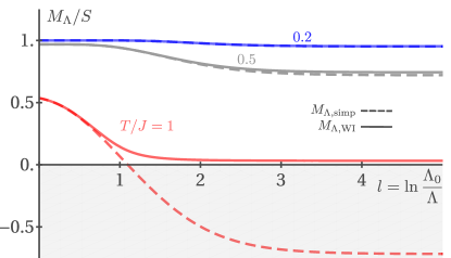
Figure 2: RG flow of the magnetization $M_{\Lambda}$ as a function of the logarithmic flow parameter $l=\ln(\Lambda_{0}/\Lambda)$ for $H/J=0.125$ and $T/J=1,0.5,0.2$ (red, gray, blue; the curves are labeled by the corresponding values of $T/J$) . The dashed lines represent the solution of the simplest truncation (67) of the flow equation for the magnetization ($M_{\Lambda,\text{simp}}$) which completely neglects self-energy and vertex corrections. The solid lines show the solution of the improved flow equation (79) ($M_{\Lambda,\text{WI}}$) which takes into account the RG flow of the magnon self-energy via the Ward identity (76). Note that $M_{\Lambda,\text{WI}}$, in contrast to $M_{\Lambda,\text{simp}}$, does not flow to unphysical negative values for high temperatures.

Obviously, for sufficiently small magnetic field and high temperatures the magnetization flows to unphysical negative values within this approximation. This is clearly an artefact of the simple approximations used to derive Eq. (67). In Sec. IV.2, we show how this problem can be cured by taking into account a Ward identity relating the magnon self-energy to the magnetization. From Eq. (67), it is furthermore straightforward to recover the RG flow equations for quantum ferromagnets derived 30 years ago in Ref. [Kopietz89, ] (see also Ref. [Kopietz89b, ]) using the momentum-shell RG technique. In this approach, the low-temperature behavior of quantum ferromagnets in $D$ dimensions is encoded in the RG flow of the following three dimensionless rescaled coupling constants:

$$t = \frac{T(a\Lambda)^{D-2}}{JSM_{\Lambda}},$$ (68a)

$$g = \frac{(a\Lambda)^{D}}{M_{\Lambda}},$$ (68b)

$$h = \frac{H}{JS}(a\Lambda)^{-2},$$ (68c)

where $\Lambda=\Lambda_{0}e^{-l}$ is the running momentum cutoff and the energy $J$ is defined byfootnoteJ

$$J=\rho_{0}/(M_{0}a^{2}).$$ (69)

Using the flow equation (67) for the scale-dependent magnetization $M_{\Lambda}$, we find that the above rescaled couplings satisfy the system of flow equations:

$$\partial_{l}t = (2-D)t+K_{D}\frac{gt}{e^{g(1+h)/t}-1},$$ (70a)

$$\partial_{l}g = -Dg+K_{D}\frac{g^{2}}{e^{g(1+h)/t}-1},$$ (70b)

$$\partial_{l}h = 2h,$$ (70c)

in agreement with the flow equations given in Refs. [Kopietz89, ; Kopietz89b, ]. By integrating these flow equations from $l=0$ up to some finite $l=l_{\ast}$ where the renormalized dimensionless temperature $t_{\ast}$ is of the order of unity, we can estimate the correlation length $\xi$ in units of the lattice spacing $a$. For $H=0$, the result is

$$\frac{\xi}{a}\propto\sqrt{\frac{JS}{T}}e^{2\pi JS^{2}/T},$$ (71)

where the precise prefactor cannot be determined with this method. Note also that flow equations similar to Eqs. (70) for quantum antiferromagnets have been obtained by Chakravarty, Halperin, and Nelson Chakravarty88 ; Chakravarty89 by applying the conventional momentum-shell RG technique to the quantum nonlinear sigma model which is believed to describe the low-energy and long-wavelength physics of quantum Heisenberg antiferromagnets in the renormalized classical regime (see Ref. [Rancon13, ] for a derivation within the FRG).

IV.2 Self-energy and vertex corrections

From Fig. 2, we see that in two dimensions the flow equation (67) implies that at sufficiently small magnetic field and large temperature the flowing magnetization $M_{\Lambda}(H,T)$ becomes negative at some finite scale $\Lambda_{c}=e^{-l_{c}}$, so that we cannot integrate the flow all the way down to $\Lambda=0$. This is of course an unphysical feature of our truncation. Within our SFRG approach we can construct a better truncation by including the flow of the magnon self-energy $\Sigma_{\Lambda}(K)$ as well as vertex corrections. However, in the presence of a finite spontaneous magnetization, the magnon spectrum must be gapless, so that the self-energy $\Sigma_{\Lambda}(K=0)$ must vanish for $H\rightarrow 0$. To implement this condition without fine-tuning the initial condition, it is crucial to truncate the infinite hierarchy of flow equations such that the Ward identity

$$\chi_{\bot}\equiv G(\bm{k}=0,i\omega=0)=\frac{M}{H}$$ (72)

is satisfied at least at the end of the flow. This identity relating the exact transverse uniform susceptibility $\chi_{\bot}$ to the exact magnetization $M$ has been discussed long time ago by Patashinskii and Prokrovskii Patashinskii73 . In Appendix C, we give a rigorous derivation of this identity using the Heisenberg equations of motion.

IV.2.1 Magnon self-energy from the Ward identity

We define the flowing magnon self-energy $\Sigma_{\Lambda}(K)$ by writing the transverse two-point vertex $\Gamma^{+-}_{\Lambda}(K)$ in the form

$$\Gamma^{+-}_{\Lambda}(K)=\frac{H+E_{\bm{k}}-i\omega}{M_{0}}+\Sigma_{\Lambda}(K),$$ (73)

so that the regularized transverse propagator is

$$G_{\Lambda}(K)=\frac{M_{0}}{H+E_{\bm{k}}-i\omega+M_{0}R_{\Lambda}^{\bot}(\bm{k})+M_{0}\Sigma_{\Lambda}(K)}.$$ (74)

Obviously, the Ward identity (72) can be implemented by demanding that the flowing transverse two-point vertex at vanishing momentum and frequency is related to the flowing magnetization via

$$\Gamma^{+-}_{\Lambda}(0)=\frac{H}{M_{\Lambda}},$$ (75)

which implies that the magnon self-energy $\Sigma_{\Lambda}(0)$ at vanishing momentum and frequency is related to the magnetization via

$$\Sigma_{\Lambda}(0)=\frac{H}{M_{\Lambda}}-\frac{H}{M_{0}}.$$ (76)

Neglecting the momentum- and frequency-dependence of the self-energy, we then obtain for the transverse single-scale propagator instead of Eq. (LABEL:eq:singlescale),

$$\dot{G}_{\Lambda}(K) = -\frac{\delta(k-\Lambda)}{\frac{H+E_{\bm{k}}-i\omega}{M_{0}}+\Sigma_{\Lambda}(0)}$$ (77)

$$= -\frac{\delta(k-\Lambda)M_{0}}{\Delta_{\Lambda}+E_{\bm{k}}-i\omega}$$

where

$$\Delta_{\Lambda}=\frac{HM_{0}}{M_{\Lambda}}$$ (78)

can be interpreted as a scale-dependent gap of the magnon dispersion. The resulting modified flow equation for the magnetization is

$$\partial_{\Lambda}M_{\Lambda}=K_{D}\frac{a^{D}\Lambda^{D-1}}{e^{\beta(\Delta_{\Lambda}+\rho_{0}\Lambda^{2})}-1}.$$ (79)

A numerical solution of this modified flow equation is shown by the solid lines in Fig. 2. Note that now the magnetization never flows to unphysical negative values. The definition (68c) of the rescaled dimensionless magnetic field should then be replaced by

$$h=\frac{H}{JM_{\Lambda}}(a\Lambda)^{-2},$$ (80)

and the modified system of flow equations for the rescaled couplings $t$, $g$, and $h$ reads

$$\partial_{l}t = (2-D)t+K_{D}\frac{gt}{e^{g(1+h)/t}-1},$$ (81a)

$$\partial_{l}g = -Dg+K_{D}\frac{g^{2}}{e^{g(1+h)/t}-1},$$ (81b)

$$\partial_{l}h = 2h+K_{D}\frac{gh}{e^{g(1+h)/t}-1}.$$ (81c)

In contrast to our earlier flow equation (70c), the renormalized magnetic field now has a nontrivial fluctuation correction.

In order to quantify the effects of additional higher order vertex corrections on the magnetization, we investigate in the following two more advanced truncations.

IV.2.2 Vertex correction from the Katanin substitution

A simple approximate method to take vertex corrections into account is the so-called Katanin substitution, which amounts to replacing the single-scale propagator in the flow equations by a total derivative, Katanin04

$$\dot{G}_{\Lambda}(K)\rightarrow\partial_{\Lambda}G_{\Lambda}(K).$$ (82)

This substitution, known from the FRG formulation of interacting Fermi systems Katanin04 ; Metzner12 , has been found to be essential to obtain meaningful results in the pseudofermion FRG approach to quantum spin systems Reuther10 ; Reuther11 ; Reuther11a ; Buessen16 . The effect of higher-order vertices is thereby partially taken into account in a weak coupling truncation. In this way, the violation of Ward identities is shifted to a higher order in the vertex expansion. Within our simple truncation the Katanin substitution amounts to replacing the single-scale propagator in Eq. (77) by

$$\dot{G}_{\Lambda}(K)\rightarrow\partial_{\Lambda}\frac{\Theta(k-\Lambda)}{\frac{H+E_{\bm{k}}-i\omega}{M_{0}}+\Sigma_{\Lambda}(0)}$$

$$=-\frac{\delta(k-\Lambda)}{\frac{H+E_{\bm{k}}-i\omega}{M_{0}}+\Sigma_{\Lambda}(0)}-\frac{\Theta(k-\Lambda)\partial_{\Lambda}\Sigma_{\Lambda}(0)}{\bigl{[}\frac{H+E_{\bm{k}}-i\omega}{M_{0}}+\Sigma_{\Lambda}(0)\bigr{]}^{2}}.$$

(83)

With this replacement the right-hand side of our truncated flow equation (64) for the magnetization becomes a total derivative. Using again the Ward identity (76) to express $\Sigma(0)$ at the end of the flow in terms of the magnetization $M$, we obtain

$$M=M_{0}-\frac{1}{N}\sum_{\bm{k}}\frac{1}{e^{\beta(HM_{0}/M+E_{\bm{k}})}-1}.$$ (84)

In one and two dimensions, the zero-field susceptibility $\chi=\lim_{H\rightarrow 0}M/H$ is expected to be finite for any non-zero temperature, so that the gap $\Delta_{\Lambda}$ approaches a finite limit for $H\rightarrow 0$. In this limit Eq. (84) reduces to the following equation for the zero-field susceptibility:

$$M_{0}=\frac{1}{N}\sum_{\bm{k}}\frac{1}{e^{\beta(M_{0}/\chi+E_{\bm{k}})}-1}.$$ (85)

At low temperatures ($T\ll V_{0})$, we can solve this equation by approximating

$$\frac{1}{e^{\beta(M_{0}/\chi+E_{\bm{k}})}-1}\approx\frac{T}{M_{0}/\chi+\rho_{0}k^{2}}$$ (86)

and imposing an ultraviolet cutoff $\Lambda_{0}$ on the momentum-integration such that $\beta\rho_{0}\Lambda_{0}^{2}=1$. Defining the energy scalefootnoteJ $J$ in terms of $\rho_{0}$ as in Eq. (69) and using the fact that at low temperatures $M_{0}\approx S$, we obtain for the susceptibility at vanishing magnetic field,

$$\chi=\frac{M_{0}}{T}e^{4\pi JS^{2}/T}.$$ (87)

The transverse correlation length $\xi(H,T)$ can be defined by writing the magnon dispersion for small momenta as

$$HM_{0}/M+E_{\bm{k}}\approx\rho_{0}(\xi^{-2}+k^{2}).$$ (88)

For $H\rightarrow 0$, this leads to the identification

$$\xi=\sqrt{\rho_{0}\chi/M_{0}}.$$ (89)

With $\chi$ given by Eq. (87), this yields

$$\frac{\xi}{a}=\sqrt{\frac{JS}{T}}e^{2\pi JS^{2}/T},$$ (90)

which agrees (up to a numerical prefactor of the order of unity) with previous one-loop calculations based on modified spin-wave theory Takahashi86 , Schwinger-Boson mean-field theory Arovas88 , and a one-loop momentum shell renormalization group calculation Kopietz89 . As shown in Ref. [Kopietz89, ], however, a more accurate two-loop calculation gives an addition factor of $T/(JS^{2})$ in front of the exponential, i.e., $\xi\propto(T/JS)^{1/2}e^{2\pi JS^{2}/T}$. Similarly, the temperature dependence of the prefactor in the expression (87) for the susceptibility is known to be modified by two-loop corrections Kopietz89 . Moreover, the one-loop approximation for the zero-field susceptibility given in Refs. [Takahashi86, ; Arovas88, ; Kopietz89, ] is a factor of $T/(JS)$ smaller than the result (87). A possible reason for this discrepancy is that in our truncation we have neglected the frequency and momentum dependence of the magnon self-energy.

Within our approach, it is possible to quantify the vertex correction which is implicitly taken into account via the Katanin substitution. Therefore we use the Ward identity (76) to express the scale-derivative of the self-energy on the right-hand side of Eq. (83) in terms of the derivative of the magnetization,

$$\partial_{\Lambda}\Sigma_{\Lambda}(0)=-\frac{H}{M_{\Lambda}^{2}}\partial_{\Lambda}M_{\Lambda}.$$ (91)

Our truncated flow equation (64) can then be written as

$$\partial_{\Lambda}M_{\Lambda} = \frac{M_{0}}{\beta N}\sum_{\bm{k},\omega}\frac{\Gamma^{+-z}_{\Lambda,{\rm Kat}}\delta(k-\Lambda)}{\Delta_{\Lambda}+E_{\bm{k}}-i\omega},$$ (92)

where the scale-dependent mixed three-point vertex is given by

$$M_{0}\Gamma^{+-z}_{\Lambda,{\rm Kat}}=\frac{1}{1+\frac{\Delta_{\Lambda}}{M_{\Lambda}}\int_{K}\frac{\Theta(\Lambda_{0}-k)\Theta(k-\Lambda)}{[\Delta_{\Lambda}+E_{\bm{k}}-i\omega]^{2}}}.\hskip 19.91692pt$$ (93)

We conclude that the Katanin substitution amounts to the assumption that the mixed three-legged vertex $\Gamma^{+-z}_{\Lambda}(-K,K,0)$ in the exact FRG flow equation (41) for the exchange field $\phi_{\Lambda}$ can be approximated by a momentum- and frequency-independent constant $\Gamma^{+-z}_{\Lambda,{\rm Kat}}$ which is linked to the flowing magnetization $M_{\Lambda}$ via Eq. (93). In Fig. 3 we show the flow of $\Gamma^{+-z}_{\Lambda,{\rm Kat}}$ in two dimensions for $T>0$ and finite magnetic field.

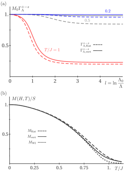
Figure 3: (a) RG flow of the vertex $\Gamma_{\Lambda}^{+-z}$ as a function of the logarithmic flow parameter $l=\ln(\Lambda_{0}/\Lambda)$ for $T/J=1,0.5,0.2$ (red, gray, blue) and $H/J=0.125$, calculated either using the Katanin substitution ($\Gamma_{\Lambda,\text{Kat}}^{+-z}$, see Eqs. (92) and (93)), or the approximate solution of the SFRG flow equations ($\Gamma_{\Lambda,\text{vert}}^{+-z}$, see Eqs. (102) and (100)). The qualitative behavior of $\Gamma_{\Lambda,\text{vert}}^{+-z}$ and $\Gamma_{\Lambda,\text{Kat}}^{+-z}$ is similar throughout the temperature range considered. (b) Resulting magnetization $M(H,T)=M_{\Lambda\rightarrow 0}(H,T)$ as a function of temperature. The dotted line represents the solution of the flow equation (79) without vertex correction where $M_{0}\Gamma_{\Lambda}^{+-z}=1$. The different magnetization curves coincide for high and low temperatures and show only small deviations in the intermediate range.

Although the vertex correction becomes important when the magnetization is significantly reduced from its initial value, the flow of the magnetization is very similar to the flow obtained without vertex correction.

IV.2.3 Vertex correction from flow equations

We have shown in the previous subsection that the Katanin substitution (83) amounts to replacing the three-legged vertex $\Gamma^{+-z}_{\Lambda}(-K,K,0)$ in the flow equation (60) for the expectation value $\phi_{\Lambda}$ of the exchange field by a momentum- and frequency-independent coupling $\Gamma^{+-z}_{\Lambda,{\rm Kat}}$ given by Eq. (93). To check the validity of this substitution, we now give an independent calculation of the vertex $\Gamma^{+-z}_{\Lambda}$. In principle, we could write down the corresponding exact flow equation, which depends on various higher-order vertices. Alternatively, we can use the Ward identity (76) to determine $\Gamma^{+-z}_{\Lambda}$ from the requirement that the flow equations for $\partial_{\Lambda}M_{\Lambda}$ and $\partial_{\Lambda}\Sigma_{\Lambda}(0)$ give consistent results. Within our cutoff scheme where only the transverse part of the exchange interaction is deformed, the exact flow equation (42) for the transverse two-point vertex reduces to

$$\partial_{\Lambda}\Sigma_{\Lambda}(0)=\Gamma^{+-z}_{\Lambda}(0,0,0)V_{0}\partial_{\Lambda}M_{\Lambda}$$

$$+\int_{Q}\dot{G}_{\Lambda}(Q)\Gamma^{++--}_{\Lambda}(0,-Q,Q,0)$$

$$-\int_{Q}\dot{G}_{\Lambda}(Q)F_{\Lambda}(Q)\Gamma^{+-z}_{\Lambda}(0,Q,-Q)\Gamma^{+-z}_{\Lambda}(-Q,0,Q).\hskip 19.91692pt$$

(94)

To simplify the calculation, we replace the vertices in the second and third lines of Eq. (94) by their initial values given by the tree approximation discussed in Appendix D, see Eq. (D 10). This amounts to neglecting the contribution involving the three-legged vertices in the last line of Eq. (94), and replacing in the second line

$$\int_{Q}\dot{G}_{\Lambda}(Q)\Gamma^{++--}_{\Lambda}(0,-Q,Q,0)\rightarrow U_{0}\int_{Q}\dot{G}_{\Lambda}(Q),$$ (95)

where the coupling constant $U_{0}$ is given by

$$U_{0}\approx\frac{H+V_{0}M_{0}}{M_{0}^{3}}.$$ (96)

Using the Ward identity in the form (91) to express $\partial_{\Lambda}\Sigma_{\Lambda}(0)$ in terms of $\partial_{\Lambda}M_{\Lambda}$, we finally obtain

$$\partial_{\Lambda}M_{\Lambda} = -\frac{U_{0}}{H/M_{\Lambda}^{2}+V_{0}\Gamma^{+-z}_{\Lambda}}\int_{K}\dot{G}_{\Lambda}(K).$$ (97)

On the other hand, for a momentum-independent three-legged vertex, the flow equation (60) for $M_{\Lambda}$ is of the form

$$\partial_{\Lambda}M_{\Lambda}=-\Gamma^{+-z}_{\Lambda}\int_{K}\dot{G}_{\Lambda}(K),$$ (98)

so that in this approximation the vertex $\Gamma^{+-z}_{\Lambda}$ satisfies the compatibility condition

$$\Gamma^{+-z}_{\Lambda}=\frac{U_{0}}{H/M_{\Lambda}^{2}+V_{0}\Gamma^{+-z}_{\Lambda}}.$$ (99)

Solving for $\Gamma^{+-z}_{\Lambda}$ we obtain

$$\Gamma^{+-z}_{\Lambda}=\left[\left(\frac{H}{2V_{0}M_{\Lambda}^{2}}\right)^{2}+\frac{U_{0}}{V_{0}}\right]^{1/2}-\frac{H}{2V_{0}M_{\Lambda}^{2}}.$$ (100)

Keeping in mind that $U_{0}/V_{0}=1/M_{0}^{2}+H/(V_{0}M^{3}_{0})$, we see that at the initial scale $\Lambda=\Lambda_{0}$ where $M_{\Lambda_{0}}=M_{0}$ the right-hand side of Eq. (100) reduces to $1/M_{0}$, while for small $M_{\Lambda}$ the vertex vanishes as

$$\Gamma^{+-z}_{\Lambda}\sim\frac{H+V_{0}M_{0}}{H}\frac{M_{\Lambda}^{2}}{M^{2}_{0}}.$$ (101)

With a sharp momentum cutoff the flow of the magnetization is therefore given by

$$\partial_{\Lambda}M_{\Lambda}=\frac{M_{0}}{\beta N}\sum_{\bm{k},\omega}\frac{\Gamma^{+-z}_{\Lambda}\delta(k-\Lambda)}{\Delta_{\Lambda}+E_{\bm{k}}-i\omega}.$$ (102)

In Fig. 3 we compare the flow of the vertex (100) with the corresponding vertex flow implied by the Katanin substitution, see Eq. (93). The qualitative behavior is similar, so that the Katanin substitution at least qualitatively takes the vertex correction due to the flow of the mixed three-point vertex into account. Figure 3(b) reveals furthermore that the resulting magnetization curves of the three different approximations used in this section do not differ significantly, indicating that the fulfilment of the Ward identity (72) is the essential feature of any of these truncations.

IV.2.4 Wave-function renormalization

Finally, let us include the wave-function renormalization factor $Z_{\Lambda}$ of the magnons which is related to the frequency-dependence of the magnon self-energy via

$$\Sigma_{\Lambda}(\bm{k},i\omega)=\Sigma_{\Lambda}(0)+M_{0}^{-1}\left(1-Z_{\Lambda}^{-1}\right)i\omega+{\cal{O}}(\omega^{2},k^{2}).$$ (103)

For our purpose it is sufficient to approximate the vertices in the exact flow equation (42) for the transverse two-point vertex by their initial values given in Appendix D. Then we obtain

$$\partial_{\Lambda}\Sigma_{\Lambda}(K)=\partial_{\Lambda}\Sigma_{\Lambda}^{a}(K)+\partial_{\Lambda}\Sigma_{\Lambda}^{b}(K),$$ (104)

with

$$\partial_{\Lambda}\Sigma^{a}_{\Lambda}(\bm{k},i\omega) = \frac{1}{\beta NM_{0}^{2}}\sum_{\bm{k}^{\prime},\omega^{\prime}}\dot{G}_{\Lambda}(\bm{k}^{\prime},i\omega^{\prime})$$

$$\times \Bigl{[}G_{1}^{-1}(\omega)+G_{1}^{-1}(\omega^{\prime})-V_{\bm{k}-\bm{k}^{\prime}}-V_{0}\Bigr{]},$$

$$\partial_{\Lambda}\Sigma^{b}_{\Lambda}(\bm{k},i\omega) = -\frac{1}{\beta NM_{0}^{2}}\sum_{\bm{k}^{\prime},\omega^{\prime}}\dot{G}_{\Lambda}(\bm{k}^{\prime},i\omega^{\prime})\frac{\beta\delta_{\omega,\omega^{\prime}}b^{\prime}}{1-\beta b^{\prime}V_{\bm{k}-\bm{k}^{\prime}}}$$

$$\times [G_{1}^{-1}(\omega)-V_{\bm{k}-\bm{k}^{\prime}}][G_{1}^{-1}(\omega^{\prime})-V_{\bm{k}-\bm{k}^{\prime}}],$$

where with our cutoff scheme

$$G_{1}^{-1}(\omega)=\frac{H+V_{0}M_{0}-i\omega}{M_{0}},$$ (107)

see Eq. (53). At low temperatures, the derivatives of the Brillouin function are exponentially small, so that the second contribution $\Sigma^{b}_{\Lambda}(\bm{k},i\omega)$ can be neglected. From the frequency-dependence of $\Sigma^{a}_{\Lambda}(\bm{k},i\omega)$, we obtain for the flowing wave-function renormalization

$$\partial_{\Lambda}Z_{\Lambda} = -\frac{Z_{\Lambda}^{2}}{M_{0}^{2}}\int_{K}\dot{G}_{\Lambda}(K)$$ (108)

$$= K_{D}\frac{(a\Lambda)^{D-1}}{M_{0}}\frac{Z_{\Lambda}^{3}}{e^{\beta Z_{\Lambda}(\Delta_{\Lambda}+\rho_{0}\Lambda^{2})}-1}.$$

In the following section, we discuss the resulting magnetization and wave-function renormalization as functions of temperature and magnetic field strength.

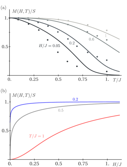
Figure 4: (a) Magnetization curve $M(T,H)$ in $D=2$ as a function of temperature obtained from the numerical integration of Eqs.  (108) and (109) for $H/J=1.0,0.6,0.2,0.05$ (top to bottom; the values of $H/J$ are written next to the curves). Here $J=\rho_{0}/(M_{0}a^{2})$ is defined in terms of the bare spin-stiffness $\rho_{0}$, see Eqs. (59) and (69). The dots are the Monte Carlo results of Ref. [Henelius00, ] for a spin $S=1/2$ Heisenberg ferromagnet with nearest neighbor exchange $J$. (b) $M(H,T)$ as a function of the magnetic field for temperatures $T/J=1,0.5,0.2$ (red, gray, blue; the values of $T/J$ are written next to the curves).

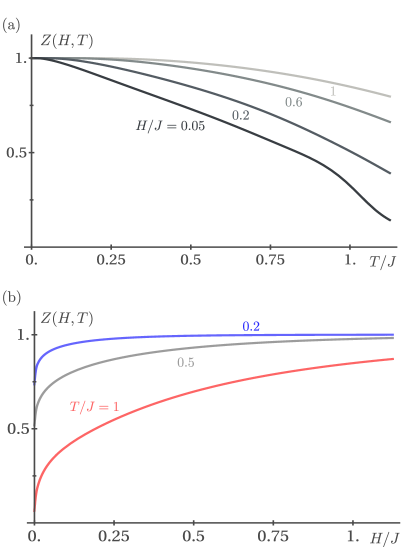
Figure 5: (a) Wave-function renormalization factor $Z(H,T)$ in $D=2$ as a function of temperature obtained from the numerical integration of Eqs. (108) and  (109) for $H/J=1.0,0.6,0.2,0.05$ (top to bottom). (b) $Z(H,T)$ as a function of magnetic field for temperatures $T/J=1,0.5,0.2$ (red, gray, blue).

IV.3 Magnetization curves

Taking into account the wave-function renormalization factor $Z_{\Lambda}$ and vertex correction given in Eq. (100), our modified flow equation for the magnetization becomes

$$\Lambda\partial_{\Lambda}M_{\Lambda}=M_{0}K_{D}\frac{Z_{\Lambda}\Gamma^{+-z}_{\Lambda}(a\Lambda)^{D}}{e^{\beta Z_{\Lambda}(\Delta_{\Lambda}+\rho_{0}\Lambda^{2})}-1},$$ (109)

which should be solved simultaneously with the flow equation (108) for the wave-function renormalization factor. Note that the vertex $\Gamma^{+-z}_{\Lambda}$ and the gap $\Delta_{\Lambda}=HM_{0}/M_{\Lambda}$ are functions of the flowing magnetization $M_{\Lambda}$, see Eqs. (100) and (78). By integrating the flow equations (109) and (108) from some large initial scale $\Lambda_{0}$ of the order of the inverse lattice spacing down to $\Lambda=0$, we obtain nonperturbative expressions for the magnetic equation of state $M(H,T)$ and the corresponding wave-function renormalization factor $Z(H,T)$, which remain well-defined in low dimensions even in the limit of vanishing magnetic field, see Figs. 4 and 5. Recall that in Eq. (69) we have defined the energy scale $J=\rho_{0}/(M_{0}a^{2})$ in terms of the bare spin stiffness footnoteJ . For low temperatures and finite magnetic field, both $M/S$ and $Z$ remain close to unity, indicating that magnons are well-defined quasiparticles. When $T/J$ is not small the magnetization and the wave-function renormalization factor both decrease. The identity (88) implies that then also the correlation length decreases. For not too small magnetic field, the quantitative agreement of our SFRG calculation with Monte Carlo simulations Henelius00 extends to temperatures of order $J$, while for $H\ll J$, our SFRG result for $M(H,T)$ agrees with the Monte Carlo results only for temperatures $T\lesssim 0.2J$. This is due to the fact that in our truncation we have neglected all terms involving the derivatives of the Brillouin function, which for $H\ll J$ is only justified for temperatures $T\ll J$. From Fig. 5 (b), we also see that for any finite magnetic field $H$ the wave-function renormalization factor $Z$ remains finite. On the other hand, $Z(H,T)$ vanishes if we take the limit $H\rightarrow 0$ for $T>0$; the corresponding steepening of the slope $\partial M(H,T)/\partial H\Huge|_{H=0}$ reflects the exponential behavior of the susceptibility calculated in Eq. (87). The fact that the Monte Carlo calculations have been performed for a nearest neighbor Heisenberg model whereas our truncation of the hierarchy of the SFRG flow equations is controlled only for long-range interactions footnoteJ does not affect the quantitative accuracy of our SFRG calculation at low temperatures because in this regime the relevant energy scale is set by the spin stiffness $\rho_{0}$ defined in terms of the small-momentum expansion (66) of the magnon dispersion. We conclude that at low temperatures the magnetization curves predicted by our SFRG approach agree with controlled Monte Carlo simulations for two-dimensional quantum Heisenberg ferromagnets Henelius00 . Similar results have been obtained with a $1/N$-expansion Timm98 , with Green function methods Junger04 , and with an exact diagonalization calculation Junger08 .

V Magnon damping due to classical longitudinal fluctuations

Let us now calculate the damping of magnons due to the coupling to classical longitudinal spin fluctuations at intermediate temperatures. This decay channel is not properly taken into account in the usual spin-wave expansion where fluctuations of the length of the magnetic moments are not treated as independent degrees of freedom Hofmann02 . For a three-dimensional ferromagnet, the leading perturbative contribution to this decay process has already been studied by VLP Vaks68b using their spin-diagrammatic approach. To obtain their result for the decay rate within our SFRG approach, we can neglect self-energy corrections to the single-scale propagator on the right-hand side of the flow equation for the self-energy $\Sigma^{b}_{\Lambda}(\bm{k},i\omega)$ in Eq. (LABEL:eq:SigmaI). The right-hand side of the flow equation is then a total derivative which can easily be integrated over the flow parameter. After analytic continuation to real frequencies we then obtain the perturbative result for the damping given by VLP Vaks68b ,

$$\gamma(\bm{k},\omega) = -M_{0}{\rm Im}\Sigma^{b}_{\Lambda}(\bm{k},\omega+i0)$$ (110)

$$= \frac{\pi b^{\prime}}{N}\sum_{\bm{k}^{\prime}}\delta(H+E_{\bm{k}^{\prime}}-\omega)\frac{(V_{\bm{k}^{\prime}}-V_{\bm{k}-\bm{k}^{\prime}})^{2}}{1-\beta b^{\prime}V_{\bm{k}-\bm{k}^{\prime}}}.\hskip 19.91692pt$$

In two dimensions, this expression is not valid for small magnetic field, because we know that self-energy corrections generate a gap in the magnon spectrum and therefore cannot be neglected. Unfortunately, the inclusion of self-energy corrections requires also a consistent renormalization of the higher-order interaction vertices which is beyond the scope of this work. A simple phenomenological way to take self-energy effects into account is to replace the bare magnetic field $H$ in Eq. (110) by the gap

$$\Delta=\frac{HM_{0}}{M(H,T)}$$ (111)

and divide the external frequency by the wave-function renormalization factor $Z$, both of which are calculated by means of our SFRG approach. This leads to the following expression for the magnon damping,

$$\gamma(\bm{k},\omega) = \frac{\pi b^{\prime}}{N}\sum_{\bm{k}^{\prime}}\delta(\Delta+E_{\bm{k}^{\prime}}-\omega/Z)\frac{(V_{\bm{k}^{\prime}}-V_{\bm{k}-\bm{k}^{\prime}})^{2}}{1-\beta b^{\prime}V_{\bm{k}-\bm{k}^{\prime}}}.$$

Formally, the renormalizations described by $\Delta$ and $Z$ can be generated by replacing the mean-field inverse propagators $G_{1}^{-1}(i\omega)$ in the second line of Eq. (LABEL:eq:SigmaI) by appropriate renormalized propagators, which amounts to assuming that the structure of renormalized vertex resembles the bare one. Evaluating $\gamma(\bm{k},\omega)$ within a small-momentum expansion, we plot in Fig. 6 the resulting spectral density function

$$S(\bm{k},\omega) =\frac{1}{\pi}\text{Im }G(\bm{k},i\omega\rightarrow\omega+i0)$$

$$=\frac{1}{\pi}\frac{M_{0}\gamma(\bm{k},\omega)}{\left[\Delta+E_{k}-\omega/Z\right]^{2}+\gamma(\bm{k},\omega)^{2}}$$ (113)

as a function of temperature and magnetic field for a generic momentum $\bm{k}_{0}$. Note that the threshold for the spectral weight is controlled by the $\delta$ function in Eq. (LABEL:eq:dampres), which sets $S(\bm{k},\omega)=0$ for $\omega<Z(\Delta+E_{\bm{k}_{0}})$. In the limit $H\rightarrow 0$, this implies that the spectral weight $S(\bm{k},\omega)$ vanishes for $\omega<ZM_{0}/\chi(T)+E_{\bm{k}_{0}}$, where $\chi(T)$ is the susceptibility for vanishing field. With increasing magnetic field and decreasing temperature the resulting quasiparticle-peaks grow and sharpen, so that the magnons are stabilized in this regime. The same holds true when the magnitude of the magnon momentum $k_{0}$ is lowered (not shown in Fig. 6). The momentum and frequency dependence of $\gamma(\bm{k},\omega)$ furthermore leads to a non-Lorentzian asymmetry of the spectral lineshape, which increases when the quasiparticle-peaks broaden.

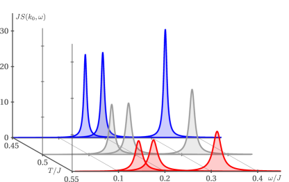
Figure 6: Spectral density function $S(\bm{k}_{0},\omega)$ as a function of frequency and temperature for $k_{0}a=0.75$ and different magnetic fields $H/J=0.001,0.01,0.1$ (from left to right). The quasiparticle peaks sharpen with increasing magnetic field strength and decreasing temperature. Note that the lineshapes of the peaks are not symmetrical around $\omega=Z\Delta+ZE_{\bm{k}_{0}}$ but show a slight asymmetry due to the $\omega$-dependence of $\gamma(\bm{k}_{0},\omega)$.

It should be emphasized that at low temperatures ($T\ll J$) the derivative $b^{\prime}$ of the Brillouin function and hence also the magnon damping in Eq. (LABEL:eq:dampres) are exponentially small. In this regime we expect that the magnon damping is dominated by two-body scattering of renormalized magnons. The proper treatment of these type of processes, taking into account that at finite temperature magnons cannot propagate over distances larger than the correlation length, is beyond the scope of this work.

VI Summary and outlook

In this work we have used the spin functional renormalization group approach (SFRG) recently proposed by two of us Krieg19 to study the thermodynamics and dynamics of two-dimensional quantum Heisenberg ferromagnets at low temperatures. We have established the precise relation between the SFRG and an old momentum-shell RG-calculationKopietz89 , and have derived the temperature dependence of the susceptibility and transverse correlation length, which agree up to a prefactor in the susceptibility with Takahashi’s modified spin-wave theory Takahashi86 and Schwinger-Boson calculations,Arovas88 respectively. Our SFRG results for the magnetic equation of state in two dimensions agrees quite well with numerical simulations. Moreover, we have also shown how the damping of transverse spin-waves due to the coupling to longitudinal spin fluctuations can be obtained within our SFRG approach. At intermediate temperatures, this damping can be substantial in two dimensions and generates an asymmetry in the spectral line shape.

This work also contains several technical advances which will be helpful for future applications of the SFRG to quantum spin systems. Of particular importance are the following three points.

1. The construction of the hybrid functional $\Gamma_{\Lambda}[\bm{m},\phi]$ in Eq. (11) which generates vertices which are irreducible in the transverse propagator line and in the longitudinal interaction line. This functional satisfies the Wetterich equation (19) and has a well-defined initial condition even if we start from a deformed Hamiltonian where the exchange interactions are completely switched off. The two-point functions generated by this functional can be identified physically with the self-energy $\Sigma_{\Lambda}(K)$ of the transverse magnons and the irreducible polarization $\Pi_{\Lambda}(K)$ of longitudinal spin fluctuations. This establishes the precise relation between our SFRG approach and the diagrammatic method for quantum spin systems developed by VLP Vaks68 ; Vaks68b and by others Izyumov88 ; Izyumov02 .

2. The use of the Ward identity (72) to obtain a closed flow equation for the magnetization. This is crucial in the regime where the spin-rotational symmetry is spontaneously broken and the magnon spectrum is gapless. The Ward identity guarantees in this case that the gap in the magnon spectrum vanishes in the entire symmetry broken phase without fine-tuning the initial conditions. Note also that, in contrast to Takahashi’s modified spin-wave theory Takahashi86 ; Takahashi87 , in our approach, we do not assume a priori that for $H=0$ the magnetization vanishes in two dimensions.

3. In a deformation scheme where initially the exchange interactions are completely switched off, the initial condition for the renormalization group flow is determined by the connected imaginary-time ordered correlation functions of a single spin in a magnetic field. The diagrammatic calculation of these correlation function using the generalized Wick theorem for spin operators derived by VLP Vaks68 ; Vaks68b are rather cumbersome. We have derived an explicit recursive form of the generalized Wick theorem for spin operators in frequency space, see Eq. (B 14), which provides us with an efficient method to calculate the higher-order connected spin correlation functions.

Another challenging problem where our SFRG approach promises to be useful is the calculation of the longitudinal part of the dynamic structure factor of an ordered ferromagnet. VLP Vaks68b suggested that for sufficiently small wave-vectors the longitudinal structure factor of an ordered ferromagnet should exhibit a diffusive peak at vanishing frequency and two inelastic peaks at frequencies corresponding to the magnon energies. However, the diagrammatic resummation within the framework of the spin-diagrammatic approach to confirm this scenario has not been found Vaks68b ; Maleev73 . Recently, it has been shown by means of a kinetic equation approach that in the absence of momentum-relaxing scattering processes (such as umklapp processes or scattering by disorder) the longitudinal structure factor of a two-dimensional ferromagnet in a magnetic field exhibits a linearly dispersing hydrodynamic sound mode at low frequencies, which is induced by fluctuations of the magnon density Rodriguez18 . In three dimensions, such a mode was also found by Izyumov et al. Izyumov02 by means of the spin-diagram technique Vaks68 ; Vaks68b ; Izyumov88 . It would be interesting to see whether such a sound-like magnon mode can also be obtained within our SFRG approach.

Finally, let us point out that our SFRG approach can be extended in many directions. Our goal is to develop our method to become a useful tool for studying various types of frustrated spin systems in the regime without long-range magnetic order. Note that in the past few years these types of systems have been studied using the so-called pseudofermion FRG Reuther10 ; Reuther11 ; Reuther11a ; Buessen16 , which relies on the represention of the spin-$1/2$ operators in terms of fermionic operators Coleman15 . The unphysical states which are introduced by this representation have to be projected out which in practice can only be achieved approximately. This problem does not arise within our SFRG approach where we directly work with the physical spin operators.

APPENDIX A: Relations between irreducible vertices and connected correlation functions

In this appendix we work out the precise relation between the irreducible vertices generated by our hybrid functional $\tilde{\Gamma}_{\Lambda}[\bm{m},\varphi]=\Gamma_{\Lambda}[\bm{m},\phi_{\Lambda}+\varphi]$ defined via Eqs. (25) and (29) on the one hand, and the connected spin correlation functions generated by $\mathcal{G}_{\Lambda}[\bm{h}]$ defined in Eq. (5). With a slight variation of the notation introduced in Eq. (21), we define the three-component field $\bm{\Phi}_{K}$ with spherical transverse components,

$$\bm{\Phi}_{K}=\left(\begin{array}[]{c}\Phi^{+}_{K}\\ \Phi^{-}_{K}\\ \Phi^{z}_{K}\end{array}\right)=\left(\begin{array}[]{c}m^{+}_{K}\\ m^{-}_{K}\\ \phi_{K}\end{array}\right),$$ (A 1)

where the spherical Fourier components $m^{\pm}_{K}$ are defined as in Eq. (27) implying $(m_{K}^{+})^{\ast}=m_{-K}^{-}$, see Eq. (28). Note that in this appendix the superscript $\alpha$ assumes the values $+,-,z$. We also introduce the conjugate three-flavor source field

$$\bm{j}_{K}=\left(\begin{array}[]{c}j^{+}_{K}\\ j^{-}_{K}\\ j^{z}_{K}\end{array}\right)=\left(\begin{array}[]{c}h^{+}_{K}\\ h^{-}_{K}\\ s_{K}\end{array}\right).$$ (A 2)

The generating functional $\Gamma_{\Lambda}[\bm{\Phi}]=\Gamma_{\Lambda}[\bm{m},\phi]$ defined in Eq. (11) can then be written as

$$\Gamma_{\Lambda}[\bm{\Phi}]=\int_{K}\bm{\Phi}_{K}^{\dagger}\bm{j}_{K}-{\cal{F}}_{\Lambda}[\bm{j}]-\frac{1}{2}\int_{K}\bm{\Phi}_{K}^{\dagger}\mathbf{R}_{\Lambda}(\bm{k})\bm{\Phi}_{K},$$ (A 3)

where the hybrid functional ${\cal{F}}_{\Lambda}[\bm{j}]={\cal{F}}_{\Lambda}[h^{+},h^{-},s]$ is defined in Eq. (6), i.e.,

$${\cal{F}}_{\Lambda}[\bm{j}] = {\cal{G}}_{\Lambda}\Bigl{[}{h}^{+}_{K},h^{-}_{K},h^{z}_{K}=-J^{z}_{\Lambda}(\bm{k})s_{K}\Bigr{]}$$ (A 4)

$$-\frac{1}{2}\int_{K}{J}^{z}_{\Lambda}(\bm{k})s_{-K}s_{K}.$$

The regulator matrix $\mathbf{R}_{\Lambda}(\bm{k})$ is diagonal in flavor space,

$$\mathbf{R}_{\Lambda}(\bm{k})=\begin{pmatrix}R^{\perp}_{\Lambda}(\bm{k})&0&0\\ 0&R^{\perp}_{\Lambda}(\bm{k})&0\\ 0&0&R^{\phi}_{\Lambda}(\bm{k})\end{pmatrix},$$ (A 5)

where the transverse and longitudinal regulators $R^{\bot}_{\Lambda}(\bm{k})$ and $R^{\phi}_{\Lambda}(\bm{k})$ in momentum space are given in Eqs. (34) and (35). To take into account that the third component $\phi_{K}$ of $\bm{\Phi}_{K}$ can have a finite expectation value, we set $\phi_{K}=\delta(K)\phi_{\Lambda}+\varphi_{K}$ and define [see Eq. (25]

$$\tilde{\Gamma}_{\Lambda}[\bm{\tilde{\Phi}}]=\Gamma_{\Lambda}[m^{+}_{K},m^{-}_{K},\phi_{K}=\delta(K)\phi_{\Lambda}+\varphi_{K}],$$ (A 6)

where the third component of

$$\bm{\tilde{\Phi}}_{K}=\left(\begin{array}[]{c}m^{+}_{K}\\ m^{-}_{K}\\ \varphi_{K}\end{array}\right)$$ (A 7)

contains the fluctuating part $\varphi_{K}$ of the longitudinal exchange field $\phi_{K}$. The expansion of $\tilde{\Gamma}_{\Lambda}[\bm{\tilde{\Phi}}]$ in powers of $\bm{\tilde{\Phi}}$ defines the irreducible hybrid vertices, see Eq. (29). Similarly, we may expand the functional ${\cal{F}}_{\Lambda}[\bm{j}]$ in powers of the sources $\bm{j}$,

$${\cal{F}}_{\Lambda}[\bm{j}] = {\cal{F}}_{\Lambda}[0]+\int_{K}G^{+-}_{\Lambda}(K)h^{-}_{-K}h^{+}_{K}+\frac{1}{2!}\int_{K}F_{\Lambda}(K)s_{-K}s_{K}$$ (A 8)

$$+ \int_{K_{1}}\int_{K_{2}}\int_{K_{3}}\delta(K_{1}+K_{2}+K_{3})F^{+-z}_{\Lambda}(K_{1},K_{2},K_{3})h^{-}_{K_{1}}h^{+}_{K_{2}}s_{K_{3}}$$

$$+ \frac{1}{3!}\int_{K_{1}}\int_{K_{2}}\int_{K_{3}}\delta(K_{1}+K_{2}+K_{3})F^{zzz}_{\Lambda}(K_{1},K_{2},K_{3})s_{K_{1}}s_{K_{2}}s_{K_{3}}+...\quad.$$

The relations between the correlation functions generated by ${\cal{F}}_{\Lambda}[\bm{j}]$ and the vertices generated by its (subtracted) Legendre transform $\tilde{\Gamma}_{\Lambda}[\bm{\tilde{\Phi}}]$ can be obtained by successive differentiation of the field-dependent relation of the Hessian matrices,

$$\left(\bm{\tilde{\Gamma}}_{\Lambda}^{\prime\prime}[\bm{\tilde{\Phi}}]+\mathbf{R}_{\Lambda}\right)_{aa^{\prime}}=\Bigl{(}\mathbf{{F}}_{\Lambda}^{\prime\prime}[\bm{j}]\Bigr{)}^{-1}_{aa^{\prime}},$$ (A 9)

where the collective labels $a=(\alpha,K)$ and $a^{\prime}=(\alpha^{\prime},K^{\prime})$ represent the flavour index $\alpha=+,-,z$ in combination with the momentum-frequency label $K=(\bm{k},i\omega)$, and the double-primes represent the second functional derivatives with respect to the corresponding fields,

$$\left(\bm{\tilde{\Gamma}}_{\Lambda}^{\prime\prime}[\bm{\tilde{\Phi}}]\right)_{aa^{\prime}} = \frac{\delta^{2}\tilde{\Gamma}_{\Lambda}[\bm{\tilde{\Phi}}]}{\delta\tilde{\Phi}_{K}^{\alpha}\delta\tilde{\Phi}_{K^{\prime}}^{\alpha^{\prime}}},$$ (A 10)

$$\Bigl{(}\mathbf{F}_{\Lambda}^{\prime\prime}[\bm{j}]\Bigr{)}_{aa^{\prime}} = \frac{\delta^{2}\mathcal{F}_{\Lambda}[\bm{j}]}{\delta j_{K}^{\alpha}\delta j_{K^{\prime}}^{\alpha^{\prime}}}.$$ (A 11)

By taking additional derivatives of Eq. (A 9) with respect to $\tilde{\Phi}_{K}^{\alpha}$ we find for the third- and fourth-order derivative tensors,

$$\left(\bm{\tilde{\Gamma}}_{\Lambda}^{(3)}[\bm{\tilde{\Phi}}]\right)_{a_{1}a_{2}a_{3}} = -\sum_{a_{1}^{\prime}a_{2}^{\prime}a_{3}^{\prime}}\left[\prod_{i=1}^{3}\left(\mathbf{F}_{\Lambda}^{\prime\prime}[\bm{j}]\right)^{-1}_{a_{i}a_{i}^{\prime}}\right]\left(\mathbf{F}_{\Lambda}^{(3)}[\bm{j}]\right)_{a_{1}^{\prime}a_{2}^{\prime}a_{3}^{\prime}},$$ (A 12)

$$\left(\bm{\tilde{\Gamma}}_{\Lambda}^{(4)}[\bm{\tilde{\Phi}}]\right)_{a_{1}a_{2}a_{3}a_{4}} = -\sum_{a_{1}^{\prime}a_{2}^{\prime}a_{3}^{\prime}a_{4}^{\prime}}\left[\prod_{i=1}^{4}\left(\mathbf{F}_{\Lambda}^{\prime\prime}[\bm{j}]\right)^{-1}_{a_{i}a_{i}^{\prime}}\right]\left(\mathbf{F}_{\Lambda}^{(4)}[\bm{j}]\right)_{a_{1}^{\prime}a_{2}^{\prime}a_{3}^{\prime}a_{4}^{\prime}}$$ (A 13)

$$+ \mathcal{S}_{a_{1},a_{2};a_{3},a_{4}}\frac{1}{2}\sum_{a_{1}^{\prime}a_{2}^{\prime}}\left(\bm{\tilde{\Gamma}}_{\Lambda}^{(3)}[\bm{\tilde{\Phi}}]\right)_{a_{1}a_{2}a_{1}^{\prime}}\left(\mathbf{F}_{\Lambda}^{\prime\prime}[\bm{j}]\right)^{-1}_{a_{1}^{\prime}a_{2}^{\prime}}\left(\bm{\tilde{\Gamma}}_{\Lambda}^{(3)}[\bm{\tilde{\Phi}}]\right)_{a_{2}^{\prime}a_{3}a_{4}}.$$

Here, the operator $\mathcal{S}_{a_{1},a_{2};a_{3},a_{4}}$ symmetrizes the expression to its right with respect to the exchange of all labels Kopietz10 , and the summation over the internal labels is defined by $\sum_{a}=\int_{K}\sum_{\alpha=+,-,z}$. By setting $\tilde{\bm{\Phi}}=0$ and $\bm{j}=0$ in Eqs. (A 12) and (A 13) we obtain the desired expansion of the three-point and four-point vertices generated by our hybrid functional $\tilde{\Gamma}_{\Lambda}[\bm{\tilde{\Phi}}]$ in powers of the correlation functions generated by ${\cal{F}}_{\Lambda}[\bm{j}]$. Using the fact that for vanishing sources

$$\left(\mathbf{F}_{\Lambda}^{\prime\prime}[0]\right)_{KK^{\prime}}^{+-}=\delta(K+K^{\prime})G^{-+}_{\Lambda}(K)=\delta(K+K^{\prime})G_{\Lambda}(-K),$$ (A 14a)

$$\left(\mathbf{F}_{\Lambda}^{\prime\prime}[0]\right)_{KK^{\prime}}^{-+}=\delta(K+K^{\prime})G^{+-}_{\Lambda}(K)=\delta(K+K^{\prime})G_{\Lambda}(K),$$ (A 14b)

$$\left(\mathbf{F}_{\Lambda}^{\prime\prime}[0]\right)_{KK^{\prime}}^{zz}=\delta(K+K^{\prime})F_{\Lambda}(K),$$ (A 14c)

where the scale-dependent transverse propagator interaction $G_{\Lambda}(K)$ is given in Eq. (30) and the longitudinal effective interaction $F_{\Lambda}(K)$ is given in Eq. (31), we obtain from Eq. (A 12) for the three-point vertices defined via the vertex expansion (29) in momentum-frequency space,

$$\Gamma_{\Lambda}^{+-z}(K_{1},K_{2},K_{3})= -G_{\Lambda}^{-1}(-K_{1})G_{\Lambda}^{-1}(K_{2})F_{\Lambda}^{-1}(K_{3})F_{\Lambda}^{+-z}(-K_{1},-K_{2},-K_{3}),$$ (A 15)

$$\Gamma_{\Lambda}^{zzz}(K_{1},K_{2},K_{3})= -\left[\prod_{i=1}^{3}F_{\Lambda}^{-1}(K_{i})\right]F_{\Lambda}^{zzz}(-K_{1},-K_{2},-K_{3}).$$ (A 16)

Using the relation (6) between the hybrid functional ${\cal{F}}_{\Lambda}[\bm{j}]$ and the generating functional ${\cal{G}}_{\Lambda}[\bm{h}]$ of the connected spin correlation functions, we can express the three-point functions $F_{\Lambda}^{+-z}(-K_{1},-K_{2},-K_{3})$ and $F_{\Lambda}^{zzz}(-K_{1},-K_{2},-K_{3})$ on the right-hand side of Eqs. (A 15) and (A 16) in terms of the connected spin correlation functions. In momentum-frequency space we obtain

$$F_{\Lambda}^{-1}(K_{3})F_{\Lambda}^{+-z}(-K_{1},-K_{2},-K_{3}) = F_{\Lambda}^{-1}(K_{3})\left(-J^{z}_{\Lambda,\bm{k_{3}}}\right)G_{\Lambda}^{+-z}(-K_{1},-K_{2},-K_{3})$$ (A 17)

$$= \left[1+J^{z}_{\Lambda,\bm{k_{3}}}\Pi_{\Lambda}(K_{3})\right]G_{\Lambda}^{+-z}(-K_{1},-K_{2},-K_{3}),$$

$$\left[\prod_{i=1}^{3}F_{\Lambda}^{-1}(K_{i})\right]F_{\Lambda}^{zzz}(-K_{1},-K_{2},-K_{3}) = \left[\prod_{i=1}^{3}\left(1+J^{z}_{\Lambda,\bm{k}_{i}}\Pi_{\Lambda}(K_{i})\right)\right]G_{\Lambda}^{zzz}(-K_{1},-K_{2},-K_{3}).$$ (A 18)

Note that the relation (A 18) between longitudinal three-point functions follows also directly from Eq. (9). Substituting Eqs. (A 17) and (A 18) into Eqs.(A 15) and (A 16), we obtain the expansion of the three-point vertices in terms of the connected spin correlation functions,

$$\Gamma_{\Lambda}^{+-z}(K_{1},K_{2},K_{3})= -G_{\Lambda}^{-1}(-K_{1})G_{\Lambda}^{-1}(K_{2})\left[1+J^{z}_{\Lambda,\bm{k_{3}}}\Pi_{\Lambda}(K_{3})\right]G^{+-z}_{\Lambda}(-K_{1},-K_{2},-K_{3}),$$ (A 19)

$$\Gamma_{\Lambda}^{zzz}(K_{1},K_{2},K_{3})= -\left[\prod_{i=1}^{3}\left(1+J^{z}_{\Lambda,\bm{k}_{i}}\Pi_{\Lambda}(K_{i})\right)\right]G_{\Lambda}^{zzz}(-K_{1},-K_{2},-K_{3}).$$ (A 20)

Analogously, using Eq.(A 13) we find for the four-point vertices,

$$\Gamma_{\Lambda}^{++--}(K_{1},K_{2},K_{3},K_{4})= -G_{\Lambda}^{-1}(-K_{1})G_{\Lambda}^{-1}(-K_{2})G_{\Lambda}^{-1}(K_{3})G_{\Lambda}^{-1}(K_{4})G_{\Lambda}^{++--}(-K_{1},-K_{2},-K_{3},-K_{4})$$

$$+\Bigl{\{}\Gamma_{\Lambda}^{+-z}(K_{1},K_{3},-K_{1}-K_{3})F(-K_{1}-K_{3})\Gamma_{\Lambda}^{+-z}(K_{2},K_{4},-K_{2}-K_{4})+(K_{3}\leftrightarrow K_{4})\Bigr{\}},$$

$$\Gamma_{\Lambda}^{+-zz}(K_{1},K_{2},K_{3},K_{4})= -G_{\Lambda}^{-1}(-K_{1})G_{\Lambda}^{-1}(K_{2})[1+J^{z}_{\Lambda,\bm{k}_{3}}\Pi(K_{3})][1+J^{z}_{\Lambda,\bm{k}_{4}}\Pi(K_{4})]G_{\Lambda}^{+-zz}(-K_{1},-K_{2},-K_{3},-K_{4})$$

$$+\Bigl{\{}\Gamma_{\Lambda}^{+-z}(K_{1},-K_{1}-K_{3},K_{3})G_{\Lambda}(-K_{1}-K_{3})\Gamma_{\Lambda}^{+-z}(-K_{2}-K_{4},K_{2},K_{4})+(K_{3}\leftrightarrow K_{4})\Bigr{\}}$$

$$+\Gamma_{\Lambda}^{zzz}(K_{3},K_{4},-K_{3}-K_{4})F_{\Lambda}(-K_{3}-K_{4})\Gamma_{\Lambda}^{+-z}(K_{1},K_{2},-K_{1}-K_{2}).$$ (A 22)

$$\Gamma_{\Lambda}^{zzzz}(K_{1},K_{2},K_{3},K_{4})= -\left[\prod_{i=1}^{4}\left(1+J^{z}_{\Lambda,\bm{k}_{i}}\Pi(K_{i})\right)\right]G_{\Lambda}^{zzzz}(-K_{1},-K_{2},-K_{3},-K_{4})$$

$$+\Bigl{\{}\Gamma_{\Lambda}^{zzz}(K_{1},K_{3},-K_{1}-K_{3})[1+J^{z}_{\Lambda,-\bm{k}_{1}-\bm{k}_{3}}\Pi(-K_{1}-K_{3})]\Gamma_{\Lambda}^{zzz}(K_{2},K_{4},-K_{2}-K_{4})\Bigr{\}},$$ (A 23)

where we have introduced the notation $\left\{f(..,K_{3},..)+(K_{3}\leftrightarrow K_{4})\right\}=\left\{f(..,K_{3},..)+f(..,K_{4},..)\right\}$ with an arbitrary function $f$.

APPENDIX B: Generalized blocks and Wick theorem for spin operators

For vanishing exchange interaction all spins are completely decoupled so that all spin correlation functions are diagonal in the site index. The on-site time-ordered connected spin correlation functions can then be expanded in frequency space as follows,

$$G^{\alpha_{1}\ldots\alpha_{n}}_{0}(\tau_{1},\ldots,\tau_{n})\equiv\langle{\cal{T}}[S^{\alpha_{1}}(\tau_{1})\ldots S^{\alpha_{n}}(\tau_{n})]\rangle_{\rm connected}$$

$$=\frac{1}{\beta^{n}}\sum_{\omega_{1}\ldots\omega_{n}}e^{-i(\omega_{1}\tau_{1}+\ldots+\omega_{n}\tau_{n})}\tilde{G}^{\alpha_{1}\ldots\alpha_{n}}_{0}(\omega_{1},\ldots,\omega_{n}).$$

(B 1)

Translational invariance in imaginary time implies that we can factor out a frequency-conserving $\delta$-function,

$$\tilde{G}^{\alpha_{1}\ldots\alpha_{n}}_{0}(\omega_{1},\ldots,\omega_{n})$$ (B 2)

$$= \delta(\omega_{1}+\cdots+\omega_{n}){G}^{\alpha_{1}\ldots\alpha_{n}}_{0}(\omega_{1},\ldots,\omega_{n}),$$

where we have introduced the discretized $\delta$-function in frequency space,

$$\delta(\omega)=\beta\delta_{\omega,0}.$$ (B 3)

In the book by Izyumov and Skryabin Izyumov88 time-ordered connected spin correlation functions ${G}^{\alpha_{1}\ldots\alpha_{n}}_{0}(\omega_{1},\ldots,\omega_{n})$ are called generalized blocks. In the local limit the longitudinal correlations are purely static and can be expressed in terms of the derivatives of the Brillouin function,

$$\tilde{G}^{zz}_{0}(\omega_{1},\omega_{2}) = \delta(\omega_{1})\delta(\omega_{2})b^{\prime},$$ (B 4)

$$\tilde{G}^{zzz}_{0}(\omega_{1},\omega_{2},\omega_{3}) = \delta(\omega_{1})\delta(\omega_{2})\delta(\omega_{3})b^{\prime\prime},$$ (B 5)

$$\tilde{G}_{0}^{zzzz}(\omega_{1},\omega_{2},\omega_{3},\omega_{4}) = \delta(\omega_{1})\delta(\omega_{2})\delta(\omega_{3})\delta(\omega_{4})b^{\prime\prime\prime}.\hskip 19.91692pt$$ (B 6)

The transverse two-spin correlation functions are

$$\tilde{G}^{+-}_{0}(\omega,\omega^{\prime}) = \delta(\omega+\omega^{\prime})G_{0}(\omega),$$ (B 7)

$$\tilde{G}^{-+}_{0}(\omega,\omega^{\prime}) = \delta(\omega+\omega^{\prime})G_{0}(-\omega),$$ (B 8)

where

$$G_{0}(\omega)=\frac{b}{H-i\omega},$$ (B 9)

and the spin-$S$ Brillouin function $b=b(\beta H)$ is given in Eq. (52). The mixed three-spin correlation function is

$$b{G}^{+-z}_{0}(\omega_{1},\omega_{2},\omega_{3})=-G_{0}(\omega_{1})G_{0}(-\omega_{2})+G_{0}(\omega_{1})\delta(\omega_{3})b^{\prime},$$

(B 10)

and the purely transverse connected four-spin correlation function is

$$b^{2}{G}^{++--}_{0}(\omega_{1},\omega_{2},\omega_{3},\omega_{4})=$$

$$-G_{0}(\omega_{1})G_{0}(\omega_{2})[G_{0}(-\omega_{3})+G_{0}(-\omega_{4})]$$

$$+G_{0}(\omega_{1})G_{0}(\omega_{2})[\delta(\omega_{1}+\omega_{3})+\delta(\omega_{1}+\omega_{4})]b^{\prime}.\hskip 19.91692pt$$ (B 11)

There is also a mixed four-spin correlation function involving two transverse and two longitudinal spin components,

$$b^{2}{G}^{+-zz}_{0}(\omega_{1},\omega_{2},\omega_{3},\omega_{4})=$$

$$G_{0}(\omega_{1})G_{0}(-\omega_{2})[G_{0}(\omega_{1}+\omega_{3})+G_{0}(\omega_{1}+\omega_{4})]$$

$$-G_{0}(\omega_{1})G_{0}(-\omega_{2})[\delta(\omega_{3})+\delta(\omega_{4})]b^{\prime}$$

$$+G_{0}(\omega_{1})\delta(\omega_{3})\delta(\omega_{4})bb^{\prime\prime}.$$ (B 12)

The above expressions for the connected spin correlation functions up to fourth order have have first been derived by VLPVaks68 , see also Ref.[Izyumov88, ]. The higher-order connected spin correlation functions can in principle be calculated diagrammatically using the generalized Wick theorem for spin operators derived by VLP Vaks68 . Since the diagrammatic approach is rather tedious, we have developed an alternative method to generate the higher-order connected spin correlation functions in frequency space based on the hierarchy of equations of motion given in Eq. (C10). Noting that in the limit of vanishing exchange couplings only the first two terms on the right-hand side of Eq. (C10) survive, and denoting the resulting local limit of the connected correlation function by

$$G^{(n,n,m)}_{0}(\omega_{1}\ldots\omega_{n};\omega_{1}^{\prime}\ldots\omega_{n}^{\prime};\omega_{1}^{\prime\prime}\ldots\omega_{m}^{\prime\prime})=G_{0}^{\overbrace{+\cdots+}^{n}\overbrace{-\cdots-}^{n}\overbrace{z\cdots z}^{m}}(\omega_{1}\ldots\omega_{n};\omega_{1}^{\prime}\ldots\omega_{n}^{\prime};\omega_{1}^{\prime\prime}\ldots\omega_{m}^{\prime\prime})$$ (B 13)

we obtain from Eq. (C10) the following expression relating the correlation function involving $2n$ transverse and $m$ longitudinal spin components to a linear combination of connected correlation functions involving at most $2n+m-1$ spins,

$$bG_{0}^{(n,n,m)}(\omega_{1}\ldots\omega_{n};\omega_{1}^{\prime}\ldots\omega_{n}^{\prime};\omega_{1}^{\prime\prime}\ldots\omega_{m}^{\prime\prime}) = -G_{0}(\omega_{1})\sum_{\nu=1}^{m}G_{0}^{(n,n,m-1)}(\omega_{1}+\omega_{\nu}^{\prime\prime},\omega_{2}\ldots\omega_{n};\omega_{1}^{\prime}\ldots\omega_{n}^{\prime};\omega_{1}^{\prime\prime}\ldots{\not{\omega}}_{\nu}^{\prime\prime}\ldots\omega_{m}^{\prime\prime})$$ (B 14)

$$+G_{0}(\omega_{1})\sum_{\nu=1}^{n}G_{0}^{(n-1,n-1,m+1)}(\omega_{2}\ldots\omega_{n};\omega_{1}^{\prime}\ldots\not{\omega}_{\nu}^{\prime}\ldots\omega_{n}^{\prime};\omega_{1}^{\prime\prime}\ldots\omega_{m}^{\prime\prime},\omega_{1}+\omega_{\nu}^{\prime}),$$

where the slashed symbol ${\not{\omega}}_{\nu}^{\prime\prime}$ in the list $\omega_{1}^{\prime\prime}\ldots{\not{\omega}}_{\nu}^{\prime\prime}\ldots\omega_{m}^{\prime\prime}$ means that ${\omega}_{\nu}^{\prime\prime}$ should be omitted. The recursion relation (B 14) can be viewed as an algebraic form of the generalized Wick theorem for spin operators. By iterating this relation, we can express $G_{0}^{(n,n,m)}(\omega_{1}\ldots\omega_{n};\omega_{1}^{\prime}\ldots\omega_{n}^{\prime};\omega_{1}^{\prime\prime}\ldots\omega_{m}^{\prime\prime})$ as a linear combination of terms involving products of the transverse propagators $G_{0}(\omega)$ and purely longitudinal blocks

$$G_{0}^{\overbrace{z\cdots z}^{k}}(\omega_{1}\ldots\omega_{k})=\left(\prod_{i=1}^{k-1}\delta(\omega_{i})\right)b^{(k-1)}$$ (B 15)

up to $k=n+m$, where $b^{(k)}$ denotes the $k$-th derivative of the Brillouin function.

The corresponding irreducible vertices can be obtained using the relations between irreducible vertices and connected spin correlation functions derived in Appendix A, see Eqs. (A 19–A 23). We find that the longitudinal vertices are simply given by the negative of the corresponding generalized blocks,

$$\Gamma^{zz}_{0}(\omega) = -\delta(\omega)b^{\prime},$$ (B 16)

$$\Gamma^{zzz}_{0}(\omega_{1},\omega_{2},\omega_{3}) = -\delta(\omega_{1})\delta(\omega_{2})b^{\prime\prime},$$ (B 17)

$$\Gamma^{zzzz}_{0}(\omega_{1},\omega_{2},\omega_{3},\omega_{4}) = -\delta(\omega_{1})\delta(\omega_{2})\delta(\omega_{3})b^{\prime\prime\prime}.\hskip 19.91692pt$$ (B 18)

The transverse two-point vertex is

$$\Gamma_{0}^{+-}(\omega)=G_{0}^{-1}(\omega)=\frac{H-i\omega}{b},$$ (B 19)

and the mixed three-point vertex is related to the mixed three-spin correlation function via

$$\Gamma_{0}^{+-z}(\omega_{1},\omega_{2},\omega_{3})=$$

$$-G_{0}^{-1}(-\omega_{1})G_{0}^{-1}(\omega_{2})G_{0}^{+-z}(-\omega_{1},-\omega_{2},-\omega_{3}),\hskip 19.91692pt$$ (B 20)

which gives

$$b\Gamma_{0}^{+-z}(\omega_{1},\omega_{2},\omega_{3})=1-G^{-1}_{0}(\omega_{2})\delta(\omega_{3})b^{\prime}.$$ (B 21)

The transverse and the mixed four-point vertices are given by

$$\Gamma_{0}^{++--}(\omega_{1},\omega_{2},\omega_{3},\omega_{4}) = -G_{0}^{-1}(-\omega_{1})G_{0}^{-1}(-\omega_{2})G_{0}^{-1}(\omega_{3})G_{0}^{-1}(\omega_{4})G^{++--}_{0}(-\omega_{1},-\omega_{2},-\omega_{3},-\omega_{4}),$$ (B 22)

$$\Gamma_{0}^{+-zz}(\omega_{1},\omega_{2},\omega_{3},\omega_{4}) = -G_{0}^{-1}(-\omega_{1})G_{0}^{-1}(-\omega_{2})G^{+-zz}_{0}(-\omega_{1},-\omega_{2},-\omega_{3},-\omega_{4})$$ (B 23)

$$+ \left\{\Gamma_{0}^{+-z}(\omega_{1},-\omega_{1}-\omega_{3},\omega_{3})G_{0}(-\omega_{1}-\omega_{3})\Gamma_{0}^{+-z}(-\omega_{2}-\omega_{4},\omega_{2},\omega_{4})+(\omega_{3}\leftrightarrow\omega_{4})\right\},$$

which gives

$$b^{2}\Gamma_{0}^{++--}(\omega_{1},\omega_{2},\omega_{3},\omega_{4})=G_{0}^{-1}(\omega_{3})+G_{0}^{-1}(\omega_{4})$$

$$-[\delta(\omega_{1}+\omega_{3})+\delta(\omega_{1}+\omega_{4})]b^{\prime}G_{0}^{-1}(\omega_{3})G_{0}^{-1}(\omega_{4}),\hskip 19.91692pt$$

(B 24)

and

$$b^{2}\Gamma^{+-zz}_{0}(\omega_{1},\omega_{2},\omega_{3},\omega_{4})=-[\delta(\omega_{3})+\delta(\omega_{4})]b^{\prime}$$

$$\hskip 28.45274pt+\delta(\omega_{3})\delta(\omega_{4})G_{0}^{-1}(\omega_{2})[2(b^{\prime})^{2}-bb^{\prime\prime}].$$ (B 25)

In a cutoff scheme where initially the exchange interaction is completely switched off, the above expressions for the vertices define the initial condition for the SFRG flow equations.

APPENDIX C: Ward identity and hierarchy of equations of motion

In the regime where the spin-rotational invariance is spontaneously broken, Goldstone’s theorem guarantees that the energy dispersion of the spin-waves is gapless for vanishing external field $H\rightarrow 0$. To construct a truncation of the SFRG flow equations which does not violate this, it is crucial to take into account an exact Ward identity forcing the vanishing of the spin-wave gap when $M$ remains finite for $H\rightarrow 0$. To derive this Ward identity, consider the imaginary time Heisenberg equation of motion for the spin operator $\bm{S}_{i}(\tau)$ with deformed Hamiltonian ${\cal{H}}_{\Lambda}={\cal{H}}_{0}+{\cal{V}}_{\Lambda}$ given by Eqs. (3) and (4) under the influence of an additional fluctuating source field $\bm{h}_{i}(\tau)$. Writing for simplicity $J^{\bot}_{ij}=J^{\bot}_{\Lambda,ij}$ and $J^{z}_{ij}=J^{z}_{\Lambda,ij}$, and choosing our coordinate system such that the uniform magnetic field $\bm{H}=H\bm{e}_{z}$ points in $z$-direction $\bm{e}_{z}$, the Heisenberg equation of motion for the spin operators $\bm{S}_{i}=S^{z}_{i}\bm{e}_{z}+\bm{S}^{\bot}_{i}=\bm{S}^{\parallel}_{i}+\bm{S}^{\bot}_{i}$ in imaginary time can be written as

$$i\partial_{\tau}\bm{S}_{i}(\tau)=\bm{S}_{i}(\tau) \times \biggl{[}\bm{H}+\bm{h}_{i}(\tau)$$ (C1)

$$-\sum_{j}\left(J^{z}_{ij}\bm{S}^{\parallel}_{j}+J^{\bot}_{ij}\bm{S}^{\bot}_{j}(\tau)\right)\biggr{]}.\hskip 19.91692pt$$

Taking the source-dependent average of both sides of Eq. (C1) we obtain

$$i\partial_{\tau}\langle\bm{S}_{i}(\tau)\rangle_{\bm{h}} = \langle\bm{S}_{i}(\tau)\rangle_{\bm{h}}\times\biggl{[}\bm{H}+\bm{h}_{i}(\tau)-\sum_{j}\left(J^{z}_{ij}\langle\bm{S}^{\parallel}_{j}(\tau)\rangle_{\bm{h}}+J^{\bot}_{ij}\langle\bm{S}^{\bot}_{j}(\tau)\rangle_{\bm{h}}\right)\biggr{]}$$ (C2)

$$- \sum_{j}\left(J^{z}_{ij}\langle\delta\bm{S}_{i}(\tau)\times\delta\bm{S}^{\parallel}_{j}(\tau)\rangle_{\bm{h}}+J^{\bot}_{ij}\langle\delta\bm{S}_{i}(\tau)\times\delta\bm{S}^{\bot}_{j}(\tau)\rangle_{\bm{h}}\right),$$

where $\delta\bm{S}_{i}(\tau)=\bm{S}_{i}(\tau)-\langle\bm{S}_{i}(\tau)\rangle_{\bm{h}}$ and the average symbol is defined as follows,

$$\langle\ldots\rangle_{\bm{h}}=\frac{{\rm Tr}\left[e^{-\beta{\cal{H}}_{0}}{\cal{T}}e^{\int_{0}^{\beta}d\tau[\sum_{i}\bm{h}_{i}(\tau)\cdot{\bm{S}}_{i}(\tau)-{\cal{V}}_{\Lambda}(\tau)]}\ldots\right]}{{\rm Tr}\left[e^{-\beta{\cal{H}}_{0}}{\cal{T}}e^{\int_{0}^{\beta}d\tau[\sum_{i}\bm{h}_{i}(\tau)\cdot{\bm{S}}_{i}(\tau)-{\cal{V}}_{\Lambda}(\tau)]}\right]}.$$ (C3)

By definition, the averages in Eq. (C2) can be expressed in terms of the derivatives of the generating functional ${\cal{G}}_{\Lambda}[\bm{h}]$ of the connected imaginary-time spin correlation functions defined in Eq. (5). It is convenient to express the part of the source field $\bm{h}_{i}(\tau)$ which is perpendicular to the external magnetic field in terms of the spherical components

$${h}^{\pm}_{i}(\tau)=\frac{1}{\sqrt{2}}\left[h^{x}_{i}(\tau)\pm ih^{y}_{i}(\tau)\right].$$ (C4)

Then Eq. (C2) reduces to the following three identities:

$$\partial_{\tau}\left[\frac{\delta{\cal{G}}_{\Lambda}}{\delta h_{i}^{z}(\tau)}\right] = \frac{\delta{\cal{G}}_{\Lambda}}{\delta h_{i}^{-}(\tau)}h_{i}^{-}(\tau)-\frac{\delta{\cal{G}}_{\Lambda}}{\delta h_{i}^{+}(\tau)}h_{i}^{+}(\tau)$$ (C5a)

$$- \sum_{j}J^{\bot}_{ij}\Biggl{[}\frac{\delta{\cal{G}}_{\Lambda}}{\delta h_{i}^{-}(\tau)}\frac{\delta{\cal{G}}_{\Lambda}}{\delta h_{j}^{+}(\tau)}-\frac{\delta{\cal{G}}_{\Lambda}}{\delta h_{i}^{+}(\tau)}\frac{\delta{\cal{G}}_{\Lambda}}{\delta h_{j}^{-}(\tau)}+\frac{\delta^{2}{\cal{G}}_{\Lambda}}{\delta h_{i}^{-}(\tau)\delta h_{j}^{+}(\tau)}-\frac{\delta^{2}{\cal{G}}_{\Lambda}}{\delta h_{i}^{+}(\tau)\delta h_{j}^{-}(\tau)}\Biggr{]},$$

$$\partial_{\tau}\left[\frac{\delta{\cal{G}}_{\Lambda}}{\delta h_{i}^{+}(\tau)}\right] = \frac{\delta{\cal{G}}_{\Lambda}}{\delta h_{i}^{+}(\tau)}[H+h_{i}^{z}(\tau)]-\frac{\delta{\cal{G}}_{\Lambda}}{\delta h_{i}^{z}(\tau)}h_{i}^{-}(\tau)$$ (C5b)

$$- \sum_{j}\Biggl{[}J^{z}_{ij}\frac{\delta{\cal{G}}_{\Lambda}}{\delta h_{i}^{+}(\tau)}\frac{\delta{\cal{G}}_{\Lambda}}{\delta h_{j}^{z}(\tau)}-J^{\bot}_{ij}\frac{\delta{\cal{G}}_{\Lambda}}{\delta h_{i}^{z}(\tau)}\frac{\delta{\cal{G}}_{\Lambda}}{\delta h_{j}^{+}(\tau)}+J^{z}_{ij}\frac{\delta^{2}{\cal{G}}_{\Lambda}}{\delta h_{i}^{+}(\tau)\delta h_{j}^{z}(\tau)}-J^{\bot}_{ij}\frac{\delta^{2}{\cal{G}}_{\Lambda}}{\delta h_{i}^{z}(\tau)\delta h_{j}^{+}(\tau)}\Biggr{]},$$

$$\partial_{\tau}\left[\frac{\delta{\cal{G}}_{\Lambda}}{\delta h_{i}^{-}(\tau)}\right] = -\frac{\delta{\cal{G}}_{\Lambda}}{\delta h_{i}^{-}(\tau)}[H+h_{i}^{z}(\tau)]+\frac{\delta{\cal{G}}_{\Lambda}}{\delta h_{i}^{z}(\tau)}h_{i}^{+}(\tau)$$ (C5c)

$$+ \sum_{j}\Biggl{[}J^{z}_{ij}\frac{\delta{\cal{G}}_{\Lambda}}{\delta h_{i}^{-}(\tau)}\frac{\delta{\cal{G}}_{\Lambda}}{\delta h_{j}^{z}(\tau)}-J^{\bot}_{ij}\frac{\delta{\cal{G}}_{\Lambda}}{\delta h_{i}^{z}(\tau)}\frac{\delta{\cal{G}}_{\Lambda}}{\delta h_{j}^{-}(\tau)}+J^{z}_{ij}\frac{\delta^{2}{\cal{G}}_{\Lambda}}{\delta h_{i}^{-}(\tau)\delta h_{j}^{z}(\tau)}-J^{\bot}_{ij}\frac{\delta^{2}{\cal{G}}_{\Lambda}}{\delta h_{i}^{z}(\tau)\delta h_{j}^{-}(\tau)}\Biggr{]}.$$

To derive the Ward identity (72), we take another functional derivative $\frac{\delta}{\delta h^{+}_{n}(\tau^{\prime})}$ of Eq. (C5c) and then set all sources equal to zero. For an isotropic ferromagnet with $J^{z}_{ij}=J^{\bot}_{ij}=-V_{ij}$ the resulting equation of motion for the transverse two-spin correlation function in real space and imaginary time can be written as

$$\partial_{\tau}G^{+-}_{in}(\tau-\tau^{\prime}) = -HG^{+-}_{in}(\tau-\tau^{\prime})+\delta_{in}\delta(\tau-\tau^{\prime})M$$ (C6)

$$+\sum_{j}V_{ij}\Bigl{[}G^{+-}_{in}(\tau-\tau^{\prime})M-G^{+-}_{jn}(\tau-\tau^{\prime})M$$

$$+G^{+-z}_{inj}(\tau,\tau^{\prime},\tau)-G^{+-z}_{jni}(\tau,\tau^{\prime},\tau)\Bigr{]},$$

where $M=\langle S^{z}_{i}(\tau)\rangle$ is the local moment for the system with deformed Hamiltonian ${\cal{H}}_{\Lambda}$ in the absence of sources, i.e. for $\bm{h}_{i}(\tau)=0$. Summing both sides of this equation over the site label $i$ and integrating $\int_{0}^{\beta}d\tau$ we see that the last term on the right-hand side vanishes due to the antisymmetry of the terms in the square braces with respect to $i\leftrightarrow j$, while the left-hand side vanishes due to the periodicity of the imaginary time spin correlation functions. Noting that the uniform transverse susceptibility is given by

$$\chi_{\bot}=G^{+-}(K=0)=\int_{0}^{\beta}d\tau\sum_{i}G^{+-}_{in}(\tau-\tau^{\prime}),$$ (C7)

we finally arrive at the Ward identity Patashinskii73 $\chi_{\bot}=M/H$, see Eq. (72) of the main text.

By successively taking higher-order derivatives of the functional relations (C5a)–(C5c), we can derive equations of motion for all higher-order connected spin correlation functions. For example, starting from the third relation (C5c) we can obtain the equations of motion for the connected spin correlation functions

$$G^{(n,n,m)}(X_{1},\cdots,X_{n};X_{1}^{\prime},\ldots,X_{n}^{\prime};X_{1}^{\prime\prime},\ldots,X_{m}^{\prime\prime})=G^{\overbrace{+\cdots+}^{n}\overbrace{-\cdots-}^{n}\overbrace{z\cdots z}^{m}}(X_{1},\cdots,X_{n};X_{1}^{\prime},\ldots,X_{n}^{\prime};X_{1}^{\prime\prime},\ldots,X_{m}^{\prime\prime})$$ (C8)

involving $2n\geq 2$ transverse and $m$ longitudinal spin components by taking $n$ derivatives with respect to the $h^{+}$-sources, $n-1$ derivatives with respect to the $h^{-}$-sources, and $m$ derivatives with respect to the $h^{z}$-sources. In Eq. (C8) the symbols $X_{i}=({\bm{r}}_{i},\tau_{i})$ are collective labels representing the lattice sites ${\bm{r}}_{i}$ and the imaginary time $\tau_{i}$. Transforming all objects to momentum-frequency space,

$$G^{(n,n,m)}(X_{1},\cdots,X_{n};X_{1}^{\prime},\ldots,X_{n}^{\prime};X_{1}^{\prime\prime},\ldots,X_{m}^{\prime\prime})=\int_{K_{1}}\ldots\int_{K_{n}}\int_{K_{1}^{\prime}}\ldots\int_{K_{n}^{\prime}}\int_{K_{1}^{\prime\prime}}\ldots\int_{K_{m}^{\prime\prime}}e^{i\sum\nolimits_{i=1}^{n}(K_{i}X_{i}+K_{i}^{\prime}X_{i}^{\prime})+i\sum\nolimits_{i=1}^{m}K_{i}^{\prime\prime}X_{i}^{\prime\prime}}$$

$$\times\delta\left(\sum\nolimits_{i=1}^{n}(K_{i}+K_{i}^{\prime})+\sum\nolimits_{i=1}^{m}K_{i}^{\prime\prime}\right)G^{(n,n,m)}(K_{1},\cdots,K_{n};K_{1}^{\prime},\ldots,K_{n}^{\prime};K_{1}^{\prime\prime},\ldots,K_{m}^{\prime\prime}),$$ (C9)

where $K_{i}X_{i}=\bm{k}_{i}\cdot\bm{r}_{i}-\omega_{i}\tau_{i}$, we obtain the following infinite hierarchy of equations,

$$(H-i\omega_{1})G^{(n,n,m)}(K_{1},K_{2}\ldots K_{n};K_{1}^{\prime}\ldots K_{n}^{\prime};K_{1}^{\prime\prime}\ldots K_{m}^{\prime\prime})=$$

$$-\sum_{\nu=1}^{m}G^{(n,n,m-1)}(K_{1}+K_{\nu}^{\prime\prime},K_{2}\ldots K_{n};K_{1}^{\prime}\ldots K_{n}^{\prime};K_{1}^{\prime\prime}\ldots{\not{K}}_{\nu}^{\prime\prime}\ldots K_{m}^{\prime\prime})$$

$$+\sum_{\nu=1}^{n}G^{(n-1,n-1,m+1)}(K_{2}\ldots K_{n};K_{1}^{\prime}\ldots\not{K}_{\nu}^{\prime}\ldots K_{n}^{\prime};K_{1}^{\prime\prime}\ldots K_{m}^{\prime\prime},K_{1}+K_{\nu}^{\prime})$$

$$+\sum_{\nu=0}^{n-1}\sum_{\mu=0}^{m}{\cal{S}}^{(+)}_{K_{2}\ldots K_{\nu+1};K_{\nu+2}\ldots K_{n}}{\cal{S}}^{(-)}_{K_{1}^{\prime}\ldots K_{\nu}^{\prime};K^{\prime}_{\nu+1}\ldots K^{\prime}_{n}}{\cal{S}}^{(z)}_{K_{1}^{\prime\prime}\ldots K_{\mu}^{\prime\prime};K^{\prime\prime}_{\mu+1}\ldots K^{\prime\prime}_{m}}\Biggl{\{}$$

$$\hskip 39.83385pt\biggl{[}J^{z}\Bigl{(}\sum\nolimits_{i=1}^{\nu}(\bm{k}_{i+1}+\bm{k}^{\prime}_{i})+\sum\nolimits_{i=1}^{\mu}\bm{k}_{i}^{\prime\prime}\Bigr{)}-J^{\bot}\Bigl{(}\bm{k}_{1}+\sum\nolimits_{i=1}^{\nu}(\bm{k}_{i+1}+\bm{k}^{\prime}_{i})+\sum\nolimits_{i=1}^{\mu}\bm{k}_{i}^{\prime\prime}\Bigr{)}\biggr{]}$$

$$\hskip 34.1433pt\times G^{(\nu,\nu,\mu+1)}\Bigl{(}K_{2}\ldots K_{\nu+1};K_{1}^{\prime}\ldots K_{\nu}^{\prime};K_{1}^{\prime\prime}\ldots K_{\mu}^{\prime\prime},-\sum\nolimits_{i=1}^{\nu}(K_{i+1}+K^{\prime}_{i})-\sum\nolimits_{i=1}^{\mu}K^{\prime\prime}_{i}\Bigr{)}$$

$$\hskip 34.1433pt\times G^{(n-\nu,n-\nu,m-\mu)}\Bigl{(}K_{1}+\sum\nolimits_{i=1}^{\nu}(K_{i+1}+K^{\prime}_{i})+\sum\nolimits_{i=1}^{\mu}K^{\prime\prime}_{i},K_{\nu+2}\ldots K_{n};K^{\prime}_{\nu+1}\ldots K^{\prime}_{n};K^{\prime\prime}_{\mu+1}\ldots K^{\prime\prime}_{m}\Bigr{)}\Biggl{\}}$$

$$+\int_{Q}[J^{z}(\bm{q})-J^{\bot}(\bm{k}_{1}+\bm{q})]G^{(n,n,m+1)}\bigl{(}K_{1}+Q,K_{2}\ldots K_{n};K_{1}^{\prime}\ldots K_{n}^{\prime};K_{1}^{\prime\prime}\ldots K_{m}^{\prime\prime},-Q\bigr{)},$$ (C10)

where the slashed symbol ${\not{K}}_{\nu}^{\prime\prime}$ in the list $K_{1}^{\prime\prime}\ldots{\not{K}}_{\nu}^{\prime\prime}\ldots K_{m}^{\prime\prime}$ means that ${K}_{\nu}^{\prime\prime}$ should be deleted from the list, and the operators ${\cal{S}}^{(\alpha)}$ (where $\alpha=+,-,z$) symmetrize all expressions with respect to permutations of the $K$-labels belonging to the same spin component, see Ref. [Kopietz10, ] for an explicit definition of these operators. To obtain the equations of motion of purely longitudinal correlation functions, we take functional derivatives of the first equation (C5a) with respect to the longitudinal sources and then set all sources equal to zero. Note that only the terms involving the second functional derivative in the second line of Eq. (C5a) survive in this limit, which in Fourier space involve a loop integral. If we deform our model such that the loop integrations are small (this is the case in the presence of a strong external magnetic field, or if the exchange interaction is long-ranged), then all terms involving loops can be dropped. We call this the tree approximation. In this limit we can solve the simplified hierarchy of flow equations recursively, because the right-hand side of the hierarchy (C10) involves correlation functions of the same order as the left-hand side with the same arguments or of lower order. In Appendix D we explicitly give the tree approximation for the vertices with up to four external legs.

APPENDIX D: Tree approximation for correlation functions and vertices

For the approximate solution of the SFRG flow equations it is convenient to include the exchange couplings between different spins at the initial scale within the tree approximation, which graphically amounts to neglecting all diagrams involving closed loops. In the spirit of VLP Vaks68 , we therefore assume that the exchange interaction is long-ranged so that its Fourier transform is dominated by momenta $|\bm{k}|\lesssim k_{0}\ll 1/a$, where $a$ is the lattice spacing. Loop integrations over momenta are then suppressed by powers of $k_{0}a$, so that perturbation theory in powers of loops is controlled by the small parameter $k_{0}a$. To leading order, we may simply neglect all loops (tree approximation). As already pointed out at the end of Appendix C, in this limit the infinite hierarchy of equations of motion decouples. To simplify our notation, let us rename here the Fourier transform of the exchange couplings as follows,

$$J^{z}(\bm{k})=-V^{z}_{\bm{k}},\;\;\;\;J^{\bot}(\bm{k})=-V^{\bot}_{\bm{k}}.$$ (D 1)

The tree approximation for the transverse propagator is

$$G_{0}(K)=G_{0}(\bm{k},i\omega)=\frac{M_{0}}{H+E_{\bm{k}}-i\omega},$$ (D 2)

where the magnetization $M_{0}$ in self-consistent mean-field approximation is defined in Eq. (50), and $E_{\bm{k}}=M_{0}(V^{z}_{0}-V^{\bot}_{\bm{k}})$ is the magnon dispersion. The longitudinal effective interaction is in tree approximation given by

$$F_{0}(K)=F_{0}(\bm{k},i\omega)=\frac{V^{z}_{\bm{k}}}{1-\delta(\omega)b^{\prime}V^{z}_{\bm{k}}},$$ (D 3)

while the tree approximation for the mixed three-spin correlation function can be written as

$$M_{0}G^{+-z}_{\rm tree}(K_{1},K_{2},K_{3})=-G_{0}(K_{1})G_{0}(-K_{2})\left\{1-\bigl{[}G^{-1}_{0}(-K_{2})+V^{\bot}_{\bm{k}_{2}}-V^{z}_{\bm{k}_{3}}\bigr{]}\frac{\delta(\omega_{3})b^{\prime}}{1-\beta b^{\prime}V^{z}_{\bm{k}_{3}}}\right\}.$$ (D 4)

Moreover, from the equation of motion (C10) we obtain for transverse four-spin correlation function in tree approximation

$$M_{0}^{2}G^{++--}_{\rm tree}(K_{1},K_{2},K_{3},K_{4})=-G_{0}(K_{1})G_{0}(K_{2})G_{0}(-K_{3})G_{0}(-K_{4})\Biggl{\{}G^{-1}_{0}(-K_{3})+V^{\bot}_{\bm{k}_{3}}-V^{z}_{\bm{k}_{1}+\bm{k}_{3}}$$

$$-\frac{\delta(\omega_{1}+\omega_{3})b^{\prime}}{1-\beta V^{z}_{\bm{k}_{1}+\bm{k}_{3}}b^{\prime}}\left[G^{-1}_{0}(-K_{3})+V^{\bot}_{\bm{k}_{3}}-V^{z}_{\bm{k}_{1}+\bm{k}_{3}}\right]\left[G^{-1}_{0}(-K_{4})+V^{\bot}_{\bm{k}_{4}}-V^{z}_{\bm{k}_{1}+\bm{k}_{3}}\right]+(K_{3}\leftrightarrow K_{4})\Biggr{\}}.$$ (D 5)

Finally, the tree approximation for the mixed four-spin correlation function can be written as

$$M_{0}^{2}G^{+-zz}_{\rm tree}(K_{1},K_{2},K_{3},K_{4})=\frac{G_{0}(K_{1})G_{0}(-K_{2})}{[1-\delta(\omega_{3})b^{\prime}V^{z}_{\bm{k}_{3}}][1-\delta(\omega_{4})b^{\prime}V^{z}_{\bm{k}_{4}}]}\Biggl{\{}\frac{G_{0}^{-1}(-K_{2})+V^{\bot}_{\bm{k}_{2}}-V^{z}_{\bm{k}_{3}+\bm{k}_{4}}}{1-\beta b^{\prime}V^{z}_{\bm{k}_{3}+\bm{k}_{4}}}\delta(\omega_{3})\delta(\omega_{4})M_{0}b^{\prime\prime}$$

$$\hskip 56.9055pt+\biggl{\{}G_{0}(K_{1}+K_{3})\Bigl{[}1+\delta(\omega_{3})b^{\prime}V^{\bot}_{\bm{k}_{1}+\bm{k}_{3}}\Bigr{]}\Bigl{[}1-\delta(\omega_{4})b^{\prime}\bigl{(}G_{0}^{-1}(-K_{2})+V^{\bot}_{\bm{k}_{2}}\bigr{)}\Bigr{]}+(K_{3}\leftrightarrow K_{4})\biggr{\}}\Biggr{\}}.$$ (D 6)

Note that for vanishing exchange couplings Eqs. (D 4)–(D 6) reduce to the corresponding generalized blocks given in Eqs. (B 10)–(B 12).

Given the connected spin correlation functions, we can construct the corresponding irreducible vertices generated by our hybrid functional $\tilde{\Gamma}_{\Lambda}[\bm{m},\varphi]$ defined via Eqs. (11) and (25) using the general relations (A 19)–(A 23) derived in Appendix A. The two-point vertices $\Gamma^{+-}_{\rm tree}(K)$ and $\Gamma^{zz}_{\rm tree}(K)$ in tree approximation are given in Eqs. (55) and (57) of the main text. Substituting the tree approximation $G^{+-z}_{\rm tree}(K_{1},K_{2},K_{3})$ given in Eq. (D 4) for the mixed three-spin correlation function on the right-hand side of Eq. (A 19), we obtain

$$M_{0}\Gamma_{\rm tree}^{+-z}(K_{1},K_{2},K_{3})=1-\left[G_{0}^{-1}(K_{2})+V^{\bot}_{{\bm{k}}_{2}}\right]\delta(\omega_{3})b^{\prime}=1-{G}_{1}^{-1}(\omega_{2})\delta(\omega_{3})b^{\prime},$$ (D 7)

where $G_{1}(\omega)$ is defined by

$$G_{0}^{-1}(K)+V^{\bot}_{\bm{k}}=\frac{H+M_{0}(V_{0}^{z}-V_{\bm{k}}^{\bot})-i\omega}{M_{0}}+V^{\bot}_{\bm{k}}=\frac{H+M_{0}V_{0}^{z}-i\omega}{M_{0}}\equiv{G}^{-1}_{1}(\omega).$$ (D 8)

Note that with the substitutions $b\rightarrow M_{0}$ and $G_{0}^{-1}(\omega_{2})\rightarrow G_{1}^{-1}(\omega_{2})$ the mixed three-legged vertex in tree approximation can be obtained from the corresponding irreducible vertex for vanishing exchange interaction given in Eq. (B 21). Next, consider the transverse four-point vertex in tree approximation, which according to Eqs. (APPENDIX A: Relations between irreducible vertices and connected correlation functions) and (D 5) is given by

$$M_{0}^{2}\Gamma_{\rm tree}^{++--}(K_{1},K_{2},K_{3},K_{4}) = G_{0}^{-1}(K_{3})+G_{0}^{-1}(K_{4})+V^{\bot}_{\bm{k}_{3}}+V^{\bot}_{\bm{k}_{4}}-V^{z}_{\bm{k}_{1}+\bm{k}_{3}}-V^{z}_{\bm{k}_{1}+\bm{k}_{4}}$$ (D 9)

$$-\left\{\frac{\delta(\omega_{1}+\omega_{3})b^{\prime}}{1-\beta V^{z}_{\bm{k}_{1}+\bm{k}_{3}}b^{\prime}}\left(G_{0}^{-1}(K_{3})+V^{\bot}_{\bm{k}_{3}}-V^{z}_{\bm{k}_{1}+\bm{k}_{3}}\right)\left(G_{0}^{-1}(K_{4})+V^{\bot}_{\bm{k}_{4}}-V^{z}_{\bm{k}_{1}+\bm{k}_{3}}\right)+(K_{3}\leftrightarrow K_{4})\right\}$$

$$+\Bigl{\{}M_{0}\Gamma^{+-z}_{\rm tree}(K_{1},K_{3},-K_{1}-K_{3})F_{0}(-K_{1}-K_{3})M_{0}\Gamma^{+-z}_{\rm tree}(K_{2},K_{4},-K_{2}-K_{4})+(K_{3}\leftrightarrow K_{4})\Bigr{\}}.\hskip 19.91692pt$$

In the last line we substitute again the tree approximation (D 7) for the three-point vertices and obtain after some re-arrangements

$$M_{0}^{2}\Gamma_{\rm tree}^{++--}(K_{1},K_{2},K_{3},K_{4}) = G_{1}^{-1}(\omega_{3})+G_{1}^{-1}(\omega_{4})-[\delta(\omega_{1}+\omega_{3})+\delta(\omega_{1}+\omega_{4})]b^{\prime}G_{1}^{-1}(\omega_{3})G_{1}^{-1}(\omega_{4}),$$ (D 10)

which again can be obtained from the corresponding expression (B 24) for vanishing exchange couplings by replacing $G_{0}(\omega)\rightarrow G_{1}(\omega)$. Finally, for the mixed four-point vertex, we obtain from Eqs. (A 22) and (D 6),

$$M_{0}^{2}\Gamma_{\rm tree}^{+-zz}(K_{1},K_{2},K_{3},K_{4}) = -\frac{G_{0}^{-1}(-K_{2})-V^{z}_{\bm{k}_{3}+\bm{k}_{4}}}{1-\beta b^{\prime}V^{z}_{\bm{k}_{3}+\bm{k}_{4}}}\delta(\omega_{3})\delta(\omega_{4})M_{0}b^{\prime\prime}$$ (D 11)

$$-G_{0}(K_{1}+K_{3})-G_{0}(K_{1}+K_{4})+G_{0}^{-1}(-K_{2})\bigl{[}G_{0}(K_{1}+K_{3})\delta(\omega_{4})+G_{0}(K_{1}+K_{4})\delta(\omega_{3})\bigr{]}b^{\prime}$$

$$+\Bigl{\{}M_{0}\Gamma^{+-z}_{\rm tree}(K_{1},-K_{1}-K_{3},K_{3})G_{0}(K_{2}+K_{4})M_{0}\Gamma^{+-z}_{\rm tree}(-K_{2}-K_{4},K_{2},K_{4})+(K_{3}\leftrightarrow K_{4})\Bigr{\}}$$

$$+M_{0}\Gamma_{\rm tree}^{zzz}(K_{3},K_{4},-K_{3}-K_{4})F_{0}(-K_{3}-K_{4})M_{0}\Gamma_{\rm tree}^{+-z}(K_{1},K_{2},-K_{1}-K_{2}).$$

Substituting Eqs (D 7) and (B 17) for the three-point vertices, we finally obtain

$$M_{0}^{2}\Gamma_{\rm tree}^{+-zz}(K_{1},K_{2},K_{3},K_{4}) = -\left[\delta(\omega_{3})[1-V^{\bot}_{\bm{k}_{2}+\bm{k}_{4}}G_{0}(K_{2}+K_{4})]+\delta(\omega_{4})[1-V^{\bot}_{\bm{k}_{2}+\bm{k}_{3}}G_{0}(K_{2}+K_{3})]\right]b^{\prime}$$ (D 12)

$$+\delta(\omega_{3})\delta(\omega_{4})G_{1}^{-1}(\omega_{2})\left[[2-V^{\bot}_{\bm{k}_{2}+\bm{k}_{4}}G_{0}(K_{2}+K_{4})-V^{\bot}_{\bm{k}_{2}+\bm{k}_{3}}G_{0}(K_{2}+K_{3})](b^{\prime})^{2}-M_{0}b^{\prime\prime}\right].\hskip 19.91692pt$$

In the limit of vanishing exchange interaction, we recover again the corresponding single-site irreducible vertex given in Eq. (B 25). In a deformation scheme where initially only the transverse exchange interaction is switched off, the tree approximation defines the initial condition for the SFRG flow provided the range of the longitudinal exchange interaction is sufficiently large so that the momentum integrations are suppressed by the inverse interaction range.

References

• (1) J. Krieg and P. Kopietz, Exact renormalization group for quantum spin systems, Phys. Rev. B 99, 060403(R) (2019).
• (2) V. G. Vaks, A. I. Larkin, and S. A. Pikin, Thermodynamics of an ideal ferromagnetic substance, Zh. Eksp. Teor. Fiz. 53, 281 (1967) [Sov. Phys. JETP 26, 188 (1968)].
• (3) V. G. Vaks, A. I. Larkin, and S. A. Pikin, Spin waves and correlation functions in a ferromagnetic, Zh. Eksp. Teor. Fiz. 53, 1089 (1967) [Sov. Phys. JETP 26, 647 (1968)].
• (4) Yu. A. Izyumov and Yu. N. Skryabin, Statistical Mechanics of Magnetically Ordered Systems, (Springer, Berlin, 1988).
• (5) J. Berges, N. Tetradis, and C. Wetterich, Non-perturbative renormalization flow in quantum field theory and statistical physics, Phys. Rep. 363, 223 (2002).
• (6) J. M. Pawlowski, Aspects of the functional renormalization group, Ann. Phys. 312, 2831 (2007).
• (7) P. Kopietz, L. Bartosch, and F. Schรผtz, Introduction to the Functional Renormalization Group, (Springer, Berlin, 2010).
• (8) W. Metzner, M. Salmhofer, C. Honerkamp, V. Meden, and K. Schรถnhammer, Functional renormalization group approach to correlated fermion systems, Rev. Mod. Phys. 84, 299 (2012).
• (9) C. Wetterich, Exact evolution equation for the effective potential, Phys. Lett. B 301, 90 (1993).
• (10) T. Machado and N. Dupuis, From local to critical fluctuations in lattice models: A nonperturbative renormalization-group approach, Phys. Rev. E 82, 041128 (2010).
• (11) A. Ranรงon and N. Dupuis, Nonperturbative renormalization group approach to the Bose-Hubbard model, Phys. Rev. B 83, 172501 (2011).
• (12) A. Ranรงon and N. Dupuis, Nonperturbative renormalization group approach to strongly correlated lattice bosons, Phys. Rev. B 84, 174513 (2011).
• (13) A. Ranรงon and N. Dupuis, Universal thermodynamics of a two-dimensional Bose gas, Phys. Rev. A 85, 063607 (2012).
• (14) A. Ranรงon and N. Dupuis, Thermodynamics of a Bose gas near the superfluid-Mott-insulator transition, Phys. Rev. A 86, 043624 (2012).
• (15) A. Ranรงon, Nonperturbative renormalization group approach to quantum XY spin models, Phys. Rev. B 89, 214418 (2014).
• (16) J. Reuther and P. Wรถlfle, $J_{1}$-$J_{2}$ frustrated two-dimensional Heisenberg model: Random phase approximation and functional renormalization group, Phys. Rev. B 81, 144410 (2010).
• (17) J. Reuther and R. Thomale, Functional renormalization group for the anisotropic triangular antiferromagnet, Phys. Rev. B 83, 024402 (2011).
• (18) J. Reuther, R. Thomale, and S. Trebst, Finite-temperature phase diagram of the Heisenberg-Kitaev model, Phys. Rev. B 84, 100406(R) (2011).
• (19) F. L. Buessen and S. Trebst, Competing magnetic orders and spin liquids in two- and three-dimensional kagome systems: Pseudofermion functional renormalization group perspective, Phys. Rev. B 94, 235138 (2016).
• (20) P. Coleman, Introduction to Many-Body Physics (Cambridge University Press, Cambridge UK, 2015).
• (21) P. Kopietz and T. Busche, Exact renormalization group flow equations for nonrelativistic fermions: Scaling toward the Fermi surface, Phys. Rev. B 64, 155101 (2001).
• (22) D. Tarasevych, J. Krieg, and P. Kopietz, A rich manโ€™s derivation of scaling laws of the Kondo model, Phys. Rev. B 98, 235133 (2018).
• (23) D. Mermin and H. Wagner, Absence of Ferromagnetism or Antiferromagnetism in One- or Two-Dimensional Isotropic Heisenberg Models, Phys. Rev. Lett. 17, 1133 (1966); Erratum ibid. 17, 1307 (1966).
• (24) C. P. Hofmann, Spontaneous magnetization of the O(3) ferromagnet at low temperatures, Phys. Rev. B 65, 094430 (2002).
• (25) M. Takahashi, Quantum Heisenberg ferromagnets in one and two dimensions at low temperature, Prog. Theor. Phys. Suppl. 87, 233 (1986).
• (26) M. Takahashi, Few-dimensional Heisenberg ferromagnets at low temperature, Phys. Rev. Lett. 58, 168 (1987).
• (27) M. Kollar, I. Spremo, and P. Kopietz, Spin-wave theory at constant order parameter, Phys. Rev. B 67, 104427 (2003).
• (28) D. P. Arovas and A. Auerbach, Functional integral theories of low-dimensional quantum Heisenberg models, Phys. Rev. B 38, 316 (1988).
• (29) A. Chubukov, Schwinger bosons and hydrodynamics of two-dimensional magnets, Phys. Rev. B 44, 12318 (1991).
• (30) A. E. Trumper, L. O. Manuel, C. J. Gazza, and H. A. Ceccatto, Schwinger-Boson Approach to Quantum Spin Systems: Gaussian Fluctuations in the โ€œNaturalโ€ Gauge, Phys. Rev. Lett. 78, 2216 (1997).
• (31) C. Timm, S. M. Girvin, P. Henelius, and A. W. Sandvik, 1/N expansion for two-dimensional quantum ferromagnets, Phys. Rev. B 58, 1464 (1998).
• (32) E. A. Ghioldi, M. G. Gonzalez, S.-S. Zhang, Y. Kamiya, L. O. Manuel, A. E. Trumper, and C. D. Batista, Dynamical structure factor of the triangular antiferromagnet: Schwinger boson theory beyond mean field, Phys. Rev. B 98, 184403 (2018).
• (33) S. V. Tyablikov, Methods in the Quantum Theory of Magnetism, (Springer, New York, 1967).
• (34) I. Junger, D. Ihle, J. Richter, and A. Klรผmper, Green-function theory of the Heisenberg ferromagnet in a magnetic field, Phys. Rev. B 70, 104419 (2004).
• (35) I. Juhรกsz Junger, D. Ihle, L. Bogacz, and W. Janke, Thermodynamics of Heisenberg ferromagnets with arbitrary spin in a magnetic field, Phys. Rev. B 77, 174411 (2008)
• (36) P. Henelius, A. W. Sandvik, C. Timm, and S. M. Girvin, Monte Carlo study of a two-dimensional quantum ferromagnet, Phys. Rev. B 61, 364 (2000).
• (37) P. Kopietz and S. Chakravarty, Low-temperature behavior of the correlation length and the susceptibility of a quantum Heisenberg ferromagnet in two dimensions, Phys. Rev. B 40, 4858 (1989).
• (38) P. Kopietz, P. Scharf, M. S. Skaf, and S. Chakravarty, The magnetic Properties of Solid 3He in Two Dimensions, Europhys. Lett. 9, 465 (1989).
• (39) F. Schรผtz and P. Kopietz, Functional renormalization group with vacuum expectation values and spontaneous symmetry breaking, J. Phys. A: Math. Gen. 39, 8205 (2006).
• (40) For a Heisenberg ferromagnet with nearest neighbor exchange $J$ the bare dispersion of long-wavelength magnons is $E_{\bm{k}}=\rho_{0}k^{2}$ with $\rho_{0}=JM_{0}a^{2}$. This is consistent with our definition $J=\rho_{0}/(M_{0}a^{2})$ in Eq.ย (69). However, as emphasized in the main text after Eq.ย (59), the tree approximation used to calculate the initial condition for our flow equations can only be justified for long-range exchange interaction. In this case $J=\rho_{0}/(M_{0}a^{2})$ simply defines the energy scale associated with the bare spin stiffness.
• (41) T. R. Morris, The exact renormalization group and approximate solutions, Int. J. Mod. Phys. A 9, 2411 (1994).
• (42) S. Chakravarty, B. I. Halperin, and D. R. Nelson, Low-temperature behavior of two-dimensional quantum antiferromagnets, Phys. Rev. Lett. 60, 1057 (1988).
• (43) S. Chakravarty, B. I. Halperin, and D. R. Nelson, Two-dimensional quantum Heisenberg antiferromagnet at low temperatures, Phys. Rev. B 39, 2344 (1989).
• (44) A. Ranรงon, O. Kodio, N. Dupuis, and P. Lecheminant, Thermodynamics in the vicinity of a relativistic quantum critical point in 2+1 dimensions, Phys. Rev. E 88, 012113 (2013).
• (45) A. Z. Patashinskii and V. L. Prokrovskii, Longitudinal susceptibility and correlations in degenerate systems, Zh. Eksp. Teor. Fiz. 64, 1445 (1973) [Sov. Phys. JETP 37, 733 (1973)].
• (46) A. A. Katanin, Fulfillment of Ward identities in the functional renormalization group approach, Phys. Rev. B 70, 115109 (2004).
• (47) Yu. A. Izyumov, N. I. Chaschin, and V. Yu. Yushankai, Longitudinal spin dynamics in the Heisenberg ferromagnet: Diagrammatic approach, Phys. Rev. B 65, 214425 (2002).
• (48) S. V. Maleev, Diffusion of magnetization in a Heisenberg ferromagnet above the Curie point, Zh. Eksp. Teor. Fiz. 65, 1237 (1973) [Sov. Phys. JETP 38, 613 (1974)].
• (49) J. F. Rodriguez-Nieva, D. Podolsky, and E. Demler, Hydrodynamic sound modes and viscous damping in a magnon fluid, arXiv:1810.12333.