Moments of nucleon generalized parton distributions from lattice QCD simulations at physical pion mass

Abstract

We present results for the moments of nucleon isovector vector and axial generalized parton distribution functions computed within lattice QCD. Three ensembles of maximally twisted mass clover-improved fermions simulated with a physical value of the pion mass are analyzed. Two of these ensembles are generated using two degenerate light quarks. A third ensemble is used having, in addition to the light quarks, strange and charm quarks in the sea. A careful analysis of the convergence to the ground state is carried out that is shown to be essential for extracting the correct nucleon matrix elements. This allows a controlled determination of the unpolarized, helicity and tensor second Mellin moments. The vector and axial-vector generalized form factors are also computed as a function of the momentum transfer square up to about 1 GeV². The three ensembles allow us to check for unquenching effects and to assess lattice finite volume effects.

I Introduction

Understanding the structure of the nucleon in terms of its fundamental constituents is considered a milestone of hadronic physics. During the past decades, parton distribution functions (PDFs) measured at experimental facilities, such as HERA, RHIC, and LHC, have provided valuable insights into the distribution of quarks and gluons within the nucleon. Better determination of PDFs has also helped interpret experimental data and provided input for ongoing and future experiments. Furthermore, the planned Electron-Ion Collider envisions a rich program of measurements, paving the way for nucleon tomography and for mapping the three-dimensional structure of the nucleon.

Obtaining these quantities from first principles is one of the main objectives of lattice QCD, which has seen remarkable progress in recent years. In particular, the recent availability of simulations at the physical values of the quark masses allows for obtaining nucleon matrix elements without the need for a chiral extrapolation, thus eliminating a major source of systematic error. In addition, theoretical progress has enabled the first exploratory study of the parton distribution functions themselves on the lattice as compared to the traditional approach of calculating their moments Ji (2013). While this is a promising approach, progress still needs to be made in order to be able to have a direct quantitative comparison with experiment. Therefore, the calculation of moments on the lattice is crucial for comparing results with experiment, especially as statistical precision for these quantities increases and remaining systematic uncertainties, such as those from the finite lattice spacing, from the finite volume, and from excited state contaminations, come under control.

The generalized parton distributions (GPDs) occur in several physical processes, such as deeply virtual Compton scattering and deeply virtual meson production. Their forward limit coincides with the usual parton distributions and their first moments are related to the nucleon form factors. Since GPDs can be accessed in high energy processes where QCD factorization applies, the amplitude can be written as a convolution of a hard perturbative kernel and the nonperturbative universal parton distributions. GPDs are defined as matrix elements of bilocal operators separated by a lightlike interval. A common approach is to proceed with an operator product expansion that leads to a tower of local operators, the nucleon matrix elements of which can be evaluated within lattice QCD. In this paper, we compute the nucleon matrix elements of the one-derivative operators

$$\mathcal{O}_{V}^{\mu\nu}= \bar{\psi}\gamma^{\{\mu}\overleftrightarrow{D}^{\nu\}}\frac{\tau^{3}}{2}\psi,$$

$$\mathcal{O}_{A}^{\mu\nu}= \bar{\psi}\gamma_{5}\gamma^{\{\mu}\overleftrightarrow{D}^{\nu\}}\frac{\tau^{3}}{2}\psi,\,\textrm{and}$$

$$\mathcal{O}_{T}^{\mu\nu\rho}= \bar{\psi}\sigma^{[\mu\{\nu]}\overleftrightarrow{D}^{\rho\}}\frac{\tau^{3}}{2}\psi,$$ (1)

where $\psi$ and $\bar{\psi}$ are light quark flavor doublets, i.e. $\bar{\psi}=(\bar{u},\bar{d})$. In this work, we consider isovector quantities, obtained using the Pauli matrix $\tau^{3}$ as in Eq. (1). The curly brackets denote symmetrization and the square brackets antisymmetrization of the enclosed indices, with subtraction of the trace implied whenever symmetrizing and:

$$\overleftrightarrow{D}_{\mu}=\frac{1}{2}(\overrightarrow{D}_{\mu}-\overleftarrow{D}_{\mu}),\,D_{\mu}=\frac{1}{2}(\nabla_{\mu}+\nabla_{\mu}^{*})$$ (2)

with $\nabla_{\mu}$ and $\nabla_{\mu}^{*}$ denoting the forward and backward derivatives on the lattice, respectively. These nucleon matrix elements can be expanded in terms of generalized form factors (GFFs), which are Lorentz invariant functions of the momentum transfer squared. At zero momentum transfer, these nucleon matrix elements yield the second Mellin moments of the unpolarized, helicity and transversity PDFs.

In this paper we use three ensembles of twisted mass fermions with two values of the lattice spacing and two physical volume sizes to compute the three second Mellin moments. We also compute the GFFs related to the vector and axial matrix elements. The parameters of the three ensembles allow us to assess volume effects and check for any indication of unquenching due to strange and charm quarks.

The remainder of this paper is organized as follows: in Sec. II we present the matrix elements used and expressions for the GFFs obtained, in Sec. III we present the methodology employed for extracting the GFFs from the lattice, details on the lattice ensembles used, and parameters of our lattice analysis, with Sec. IV detailing the renormalization procedure employed. In Sec. V we provide our results, and in Sec. VI we give our conclusions.

II Matrix elements

We consider the nucleon matrix elements $\langle N(p^{\prime},s^{\prime})|\mathcal{O}^{\mu\nu}_{\mathcal{H}}|N(p,s)\rangle$ of the three one-derivative operators of Eq. (1) where $s$ and $p$ ($s^{\prime}$ and $p^{\prime}$) are the initial (final) spin and momentum of the nucleon, and $\mathcal{H}$ denotes the $\gamma$ structure corresponding to the vector ($V$), axial ($A$) and tensor ($T$) operators. In the isovector combination, the disconnected contributions cancel, leaving only connected contributions. The nucleon matrix elements of the operators of Eq. (1) can be written in terms of the generalized form factors as follows:

$$\langle N(p^{\prime},s^{\prime})|\mathcal{O}_{V}^{\mu\nu}|N(p,s)\rangle=\bar{u}_{N}(p^{\prime},s^{\prime})\frac{1}{2}\Bigl{[} A_{20}(q^{2})\,\gamma^{\{\mu}P^{\nu\}}+B_{20}(q^{2})\,\frac{i\sigma^{\{\mu\alpha}q_{\alpha}P^{\nu\}}}{2m_{N}}+C_{20}(q^{2})\,\frac{1}{m_{N}}q^{\{\mu}q^{\nu\}}\Bigr{]}u_{N}(p,s),$$

$$\langle N(p^{\prime},s^{\prime})|\mathcal{O}_{A}^{\mu\nu}|N(p,s)\rangle=\bar{u}_{N}(p^{\prime},s^{\prime})\frac{i}{2}\Bigl{[} \tilde{A}_{20}(q^{2})\,\gamma^{\{\mu}P^{\nu\}}\gamma^{5}+\tilde{B}_{20}(q^{2})\,\frac{q^{\{\mu}P^{\nu\}}}{2m_{N}}\gamma^{5}\Bigr{]}u_{N}(p,s),\,$$

$$\langle N(p^{\prime},s^{\prime})|\mathcal{O}_{T}^{\mu\nu\rho}|N(p,s)\rangle=\bar{u}_{N}(p^{\prime},s^{\prime})\frac{1}{2}\Bigl{[} A_{T20}(q^{2})\,i\sigma^{[\mu\{\nu]}P^{\rho\}}+\tilde{A}_{T20}(q^{2})\,\frac{P^{[\mu}q^{\{\nu]}P^{\rho\}}}{m_{N}^{2}}+$$

$$B_{T20}(q^{2})\,\frac{\gamma^{[\mu}q^{\{\nu]}P^{\rho\}}}{2m_{N}}+\tilde{B}_{T20}(q^{2})\,\frac{\gamma^{[\mu}P^{\{\nu]}q^{\rho\}}}{m_{N}}\Bigr{]}u_{N}(p,s),$$ (3)

where $u_{N}$ are nucleon spinors. $q=p^{\prime}-p$ is the momentum transfer, $P=(p^{\prime}+p)/2$, and $m_{N}$ is the nucleon mass. For zero momentum transfer, i.e. $p=p^{\prime}$, we have:

$$\langle N(p,s^{\prime})|\mathcal{O}_{V}^{\mu\nu}|N(p,s)\rangle =\frac{1}{2}A_{20}(0)\llangle\gamma^{\{\mu}p^{\nu\}}\rrangle,$$

$$\langle N(p,s^{\prime})|\mathcal{O}_{A}^{\mu\nu}|N(p,s)\rangle =\frac{i}{2}\tilde{A}_{20}(0)\llangle\gamma^{\{\mu}p^{\nu\}}\gamma^{5}\rrangle,\,$$

$$\langle N(p,s^{\prime})|\mathcal{O}_{T}^{\mu\nu\rho}|N(p,s)\rangle =\frac{i}{2}A_{T20}(0)\llangle\sigma^{[\mu\{\nu]}p^{\rho\}}\rrangle,$$ (4)

where we use the shorthand notation $\llangle\cdot\rrangle$ to denote an enclosed quantity between nucleon spinors $\bar{u}_{N}$ and $u_{N}$. The generalized form factors in the forward limit are related to the isovector momentum fraction, helicity and transversity moments via $\langle x\rangle_{u-d}=A_{20}(0)$, $\langle x\rangle_{\Delta u-\Delta d}=\tilde{A}_{20}(0)$, and $\langle x\rangle_{\delta u-\delta d}=A_{T20}(0)$.

III Methodology

III.1 Gauge ensembles

We use three gauge ensembles with the parameters listed in Table 1. Two ensembles are generated with two mass degenerate ($\textrm{N}_{\textrm{f}}{=}2$) up and down quarks with their mass tuned to reproduce the physical pion mass Abdel-Rehim et al. (2017) using two lattice volumes of $48^{3}\times 96$ and $64^{3}\times 128$ allowing one to test for finite volume dependence. We will refer to these ensembles as the small $\textrm{N}_{\textrm{f}}{=}2$ ensemble and large $\textrm{N}_{\textrm{f}}{=}2$ ensemble in addition to the identifier in the first column of Table 1. The third ensemble is generated on a lattice of $64^{3}\times 128$ Alexandrou et al. (2018a) with two degenerate light quarks and the strange and charm quarks in the sea ($\textrm{N}_{\textrm{f}}{=}2{+}1{+}1$) with masses tuned to reproduce respectively, the physical mass of the pion, kaon and D_s-meson, keeping the ratio of charm to strange quark mass $m_{c}/m_{s}\simeq 11.8$ Aoki et al. (2019). For the valence strange and charm quarks we use Osterwalder-Seiler fermions Osterwalder and Seiler (1978) with masses tuned to reproduce the mass of the $\Omega^{-}$ and the $\Lambda^{+}_{c}$ baryons Alexandrou and Kallidonis (2017), respectively. We will refer to this ensemble simply as the $\textrm{N}_{\textrm{f}}{=}2{+}1{+}1$ ensemble, and to all three ensembles used as physical point ensembles. The lattice spacing $a$ is determined using the nucleon mass. The procedure employed to determine $a$ is outlined in Ref. Alexandrou et al. (2018b).

These ensembles use the twisted mass fermion discretization scheme Frezzotti et al. (2001); Frezzotti and Rossi (2004a) and include a clover term Sheikholeslami and Wohlert (1985). Twisted mass fermions (TMF) provide an attractive formulation for lattice QCD allowing for automatic ${\cal O}(a)$ improvement Frezzotti and Rossi (2004a) of physical observables, an important property for evaluating the quantities considered here. The clover term added to the TMF action allows for reduced $\mathcal{O}(a^{2})$ breaking effects between the neutral and charged pions Abdel-Rehim et al. (2017). This leads to the stabilization of physical point simulations while retaining at the same time the particularly significant ${\cal O}(a)$ improvement that the TMF action features. For more details on the TMF formulation see Refs. Frezzotti and Rossi (2004b); Frezzotti et al. (2006); Boucaud et al. (2008) and for the simulation strategy Refs. Chiarappa et al. (2007); Abdel-Rehim et al. (2017, 2015); Alexandrou et al. (2018a).

Table 1: Simulation parameters for the $\textrm{N}_{\textrm{f}}{=}2{+}1{+}1$ Alexandrou et al. (2018a) and $\textrm{N}_{\textrm{f}}{=}2$ Abdel-Rehim et al. (2017) ensembles used in this work. When two errors are given, the first error is statistical and the second is systematic. The lattice spacing is determined using the nucleon mass, as explained in Ref. Alexandrou and Kallidonis (2017) for the cA2.09.48 ensemble and in Ref. Alexandrou et al. (2018b) for the cB211.072.64 ensemble. For the $\textrm{N}_{\textrm{f}}{=}2$ ensembles, the systematic error in the lattice spacing is due to the fact that the pion mass is underestimated and an interpolation is carried out using one-loop chiral perturbation theory to interpolate to the physical pion mass. More details can be found in Ref. Alexandrou et al. (2018b). The systematic error in the pion mass when expressed in physical units is due to the error in the lattice spacing. The volume given in the fifth column is in lattice units.

Ensemble	$c_{\rm SW}$		$\beta$		Nf	Vol.		$m_{\pi}L$	$a$ [fm]		$m_{N}/m_{\pi}$	$am_{\pi}$	$am_{N}$	$m_{\pi}$ [GeV]		$L$ [fm]
cB211.072.64	1.	69	1.	778	2+1+1	$64^{3}$$\times$	$128$	3.62	0.	0801(4)	6.74(3)	0.05658(6)	0.3813(19)	0.	1393(7)	5.12(3)
cA2.09.64	1.	57551	2.	1	2	$64^{3}$$\times$	$128$	3.97	0.	0938(3)(1)	7.14(4)	0.06193(7)	0.4421(25)	0.	1303(4)(2)	6.00(2)
cA2.09.48	1.	57551	2.	1	2	$48^{3}$$\times$	$96$	2.98	0.	0938(3)(1)	7.15(2)	0.06208(2)	0.4436(11)	0.	1306(4)(2)	4.50(1)

III.2 Correlation functions

Extraction of the nucleon matrix elements on the lattice proceeds with the evaluation of two- and three-point correlation functions. All expressions that follow are in Euclidean space. The three-point functions are given by

$$C^{\mu\nu}(\Gamma;\vec{q},\vec{p}\,^{\prime};t_{s},t_{\rm ins},t_{0}){=}\sum_{\vec{x}_{\rm ins},\vec{x}_{s}}e^{i(\vec{x}_{\rm ins}{-}\vec{x}_{0})\cdot\vec{q}}e^{-i(\vec{x}_{s}{-}\vec{x}_{0})\cdot\vec{p}\,^{\prime}}{\times}$$

$$\textrm{Tr}\left[\Gamma\langle J_{N}(t_{s},\vec{x}_{s})\mathcal{O}_{\mathcal{H}}^{\mu\nu}(t_{\rm ins},\vec{x}_{\rm ins})\bar{J}_{N}(t_{0},\vec{x}_{0})\rangle\right],$$ (5)

where $q=p^{\prime}-p$ is the momentum transfer. We give the general expressions for the matrix elements and corresponding correlation functions using any operator insertion $\mathcal{O}_{\mathcal{H}}^{\mu\nu}$ with $\mu\nu$ arbitrary with the understanding that for the tensor operator there is an additional index $\rho$. For the case of the moment of the tensor PDF, where we need a third index, we will explicitly include all indices. The initial coordinates $x_{0}$ are referred to as the source position, $x_{\rm ins}$ as the insertion, and $x_{s}$ as the sink. $\Gamma$ is a projector acting on spin indices, and we will use either the unpolarized $\Gamma_{0}{=}\frac{1}{2}(1{+}\gamma_{0})$ or the three polarized $\Gamma_{k}{=}i\gamma_{5}\gamma_{k}\Gamma_{0}$ combinations. For $J_{N}$, we use the standard nucleon interpolating operator:

$$J_{N}(\vec{x},t)=\epsilon^{abc}u^{a}(x)[u^{\intercal b}(x)\mathcal{C}\gamma_{5}d^{c}(x)]\,,$$ (6)

where $u$ and $d$ are up- and down-quark spinors and $\mathcal{C}{=}\gamma_{0}\gamma_{2}$ is the charge conjugation matrix. Inserting a complete set of states in Eq. (5), one obtains a tower of hadron matrix elements with the quantum numbers of the nucleon multiplied by overlap terms and time dependent exponentials. For large enough time separations, the excited state contributions are suppressed compared to the nucleon ground state and one can then extract the desired matrix element. Knowledge of two-point functions is required in order to cancel time dependent exponentials and overlaps. They are given by

$$C(\Gamma_{0},\vec{p};t_{s},t_{0}){=}\sum_{\vec{x}_{s}}e^{{-}i(\vec{x}_{s}{-}\vec{x}_{0})\cdot\vec{p}}\times$$

$$\textrm{Tr}\left[\Gamma_{0}{\langle}J_{N}(t_{s},\vec{x}_{s})\bar{J}_{N}(t_{0},\vec{x}_{0}){\rangle}\right].$$ (7)

In order to increase the overlap of the interpolating operator $J_{N}$ with the proton state and thus decrease overlap with excited states we use Gaussian smeared quark fields via Alexandrou et al. (1994); Gusken (1990),

$$\psi_{\rm smear}^{a}(t,{\vec{x}}) =\sum_{\vec{y}}F^{ab}({\vec{x}},{\vec{y}};U(t))\ \psi^{b}(t,{\vec{y}})\,,$$ (8)

$$F =(\mathbbm{1}+{\alpha}H)^{n}\,,$$

$$H({\vec{x}},{\vec{y}};U(t)) =\sum_{i=1}^{3}[U_{i}(x)\delta_{x,y-\hat{\imath}}+U_{i}^{\dagger}(x-\hat{\imath})\delta_{x,y+\hat{\imath}}],$$ (9)

with APE smearing Albanese et al. (1987) applied to the gauge fields $U_{\mu}$ entering the Gaussian smearing hopping matrix $H$. For the APE smearing Albanese et al. (1987) we use 50 iteration steps and $\alpha_{\textrm{APE}}{=}0.5$. The Gaussian smearing parameters are tuned to yield approximately a root mean square radius for the nucleon of about 0.5 fm, which has been found to yield early convergence of the nucleon two-point functions to the nucleon mass. This can be achieved by a combination of the smearing parameters $\alpha$ and $n$. We use $\alpha$=0.2 and $n$=125 for the $\textrm{N}_{\textrm{f}}{=}2{+}1{+}1$ ensemble, and $\alpha$=0.2 and 4.0 and $n$=90 and 50 for the large and small $\textrm{N}_{\textrm{f}}{=}2$ ensembles respectively.

III.3 Extraction of matrix element

In order to cancel time dependent exponentials and unknown overlaps of the interpolating fields with the physical state one constructs appropriate ratios of three- to two-point functions. We consider an optimized ratio constructed such that the two-point functions entering in the ratio utilize the shortest possible time separation to keep the statistical noise minimal as well as benefit from correlations. The ratio Alexandrou et al. (2013); Alexandrou et al. (2011a); Alexandrou et al. (2006) used is given by

$$R^{\mu\nu}(\Gamma;\vec{p}\,^{\prime},\vec{p};t_{s},t_{\textrm{ins}})=\frac{C^{\mu\nu}(\Gamma;\vec{p}\,^{\prime},\vec{p};t_{s},t_{\textrm{ins}})}{C(\Gamma_{0};\vec{p}\,^{\prime};t_{s})}\times$$

$$\sqrt{\frac{C(\Gamma_{0},\vec{p};t_{s}{-}t_{\textrm{ins}})C(\Gamma_{0},\vec{p}\,^{\prime};t_{\textrm{ins}})C(\Gamma_{0},\vec{p}\,^{\prime};t_{s})}{C(\Gamma_{0},\vec{p}\,^{\prime};t_{s}{-}t_{\textrm{ins}})C(\Gamma_{0},\vec{p};t_{\textrm{ins}})C(\Gamma_{0},\vec{p};t_{s})}}\,,$$ (10)

where from now on $t_{s}$ and $t_{\textrm{ins}}$ are taken to be relative to the source $t_{0}$, i.e. we assume $t_{0}$=0 without loss of generality. In the limit of large time separations, $(t_{s}{-}t_{\rm ins})\gg a$ and $t_{\textrm{ins}}\gg a$, the lowest state dominates and the ratio becomes time independent

$$R^{\mu\nu}(\Gamma;\vec{p}\,^{\prime},\vec{p};t_{s},t_{\rm ins})\xrightarrow[t_{\textrm{ins}}\gg a]{t_{s}-t_{\textrm{ins}}\gg a}\Pi^{\mu\nu}(\Gamma;\vec{p}\,^{\prime},\vec{p})\,.$$ (11)

The generalized form factors are then extracted from linear combinations of $\Pi^{\mu\nu}(\Gamma;\vec{p}\,^{\prime},\vec{p})$. In our approach, we use sequential inversions through the sink, fixing the sink momentum $\vec{p}^{\prime}$=0, which implies that the source momentum is fixed via momentum conservation to $\vec{p}$=$-\vec{q}$. The general expressions relating $\Pi^{\mu\nu}(\Gamma;\vec{q})$ to the generalized form factors are provided in Appendix A. For the special case of zero momentum transfer $\vec{q}=0$, the expressions of Appendix A simplify to

$$\Pi^{00}_{V}(\Gamma_{0}) =-\frac{3m_{N}}{4}\langle x\rangle_{u-d},$$

$$\Pi^{kk}_{V}(\Gamma_{0}) =-\frac{m_{N}}{4}\langle x\rangle_{u-d},$$

$$\Pi^{j0}_{A}(\Gamma_{k}) =-\frac{im_{N}}{2}\delta_{jk}\langle x\rangle_{\Delta u-\Delta d},$$

$$\Pi^{\mu\nu\rho}_{T}(\Gamma_{k}) =i\epsilon_{\mu\nu\rho k}\frac{m_{N}}{8}(2\delta_{0\rho}-\delta_{0\mu}-\delta_{0\nu})\langle x\rangle_{\delta u-\delta d},$$ (12)

with $j,k{=}1,2,3$ and $\mu,\nu,\rho{=}0,1,2,3$. All expressions are given in Euclidean space.

The GFFs, given in Appendix A, depend only on the momentum transfer squared ($Q^{2}=-q^{2}$), while $\Pi^{\mu\nu}(\Gamma;\vec{q})$ depends on $\vec{q}$. The system is therefore overconstrained, and thus for extracting the GFFs, we form the matrix $\mathcal{G}$ defined by

$$\Pi^{\mu\nu}(\Gamma;\vec{q})=\mathcal{G}^{\mu\nu}(\Gamma;\vec{q})F(Q^{2}),$$ (13)

where $\mathcal{G}$ is an array of kinematic coefficients given in the expressions in Appendix A and $F$ is the vector of GFFs. For example for the vector operator ${\cal O}_{V}^{\mu\nu}$, $F^{\intercal}=(A_{20},B_{20},C_{20})$ and thus $\mathcal{G}$ is an $N\times 3$ matrix where $N$ is the number of elements contributing to a given value of $Q^{2}$. To obtain $F$, we will use the singular value decomposition (SVD) of $\mathcal{G}$, combined with three methods for the identification of excited states.

III.4 Treatment of excited states

Ensuring that the asymptotic behavior of Eq. (11) holds is a delicate process. This is because the statistical noise exponentially increases with increasing sink-source separation $t_{s}$. In our analysis, we use three methods to study the dependence of the three- and two-point correlation functions on $t_{s}$ and $t_{s}-t_{\textrm{ins}}$. This allows us to study the effect of excited states and thus better identify the convergence to the desired nucleon matrix element. The methods employed are as follows:

Plateau method: In this method we use the ratio in Eq. (10) in search of a time-independent window (plateau) and extract a value by fitting to a constant. We then seek convergence of the extracted plateau value as we increase $t_{s}$ that then produces the desired matrix element.

Two-state method: Within this method, we fit the two- and three-point functions keeping terms up to the first excited state, namely we use

$$C(\vec{q},t_{s})=c_{0}(\vec{q})e^{-E_{N}(\vec{q})t_{s}}+c_{1}(\vec{q})e^{-E^{*}(\vec{q})t_{s}}\,,$$ (14)

$$C^{\mu\nu}(\Gamma;\vec{q};t_{s},t_{\rm ins}) =A_{00}^{\mu\nu}(\Gamma,\vec{q})e^{-m_{N}(t_{s}-t_{\rm ins})-E_{N}(\vec{q})t_{\rm ins}}$$

$$+A_{01}^{\mu\nu}(\Gamma,\vec{q})e^{-m_{N}(t_{s}-t_{\rm ins})-E^{*}(\vec{q})t_{\rm ins}}$$

$$+A_{10}^{\mu\nu}(\Gamma,\vec{q})e^{-m_{N}^{*}(t_{s}-t_{\rm ins})-E_{N}(\vec{q})t_{\rm ins}}$$

$$+A_{11}^{\mu\nu}(\Gamma,\vec{q})e^{-m_{N}^{*}(t_{s}-t_{\rm ins})-E^{*}(\vec{q})t_{\rm ins}},$$ (15)

where $m_{N}$ ($m_{N}^{*}$) and $E_{N}(\vec{q})$ ($E^{*}(\vec{q})$) are the mass and energy of the ground (first excited) state with momentum $\vec{q}$, respectively. The ground state corresponds to a single particle, so its energy at finite momentum is given by the continuum dispersion relation, $E_{N}(\vec{q})=\sqrt{\vec{q}^{2}+m_{N}^{2}}$, where $\vec{q}=\frac{2\pi}{L}\vec{n}$ with $\vec{n}$ a lattice vector with components $n_{i}\in(-\frac{L}{2a},\frac{L}{2a}]$. In Appendix B we check that the continuum dispersion relation is satisfied for all $Q^{2}$ values considered in this work. The first excited state, on the other hand, is allowed to be a two-particle state, although we expect the overlap to be volume suppressed. We fit the two-point function at zero momentum and the two-point function with momentum $\vec{q}$ yielding the fit parameters $m_{N}$, $m_{N}^{*}$, $E^{*}(\vec{q})$, $c_{0}(\vec{0})$, $c_{1}(\vec{0})$, $c_{0}(\vec{q})$, and $c_{1}({\vec{q}})$. The three-point function is then fitted for the four fit parameters $A_{00}$, $A_{01}$, $A_{10}$, and $A_{11}$. For extracting the moments in the case of zero momentum transfer, the two-point function fit reduces to four parameters and the three-point function fit to three. The errors of the fit parameters of the two-point functions are propagated by carrying out the fits within the resampling method used for each ensemble, i.e. within jackknife for the case of the $\textrm{N}_{\textrm{f}}{=}2{+}1{+}1$ ensemble for which all results are obtained on the same configurations, and within a bootstrap for the $\textrm{N}_{\textrm{f}}{=}2$ ensembles (see Table 2). The desired matrix element is then given by

$$\Pi^{\mu\nu}(\Gamma;\vec{q})=\frac{A_{00}^{\mu\nu}(\Gamma,\vec{q})}{\sqrt{c_{0}(0)c_{0}(\vec{q})}}.$$ (16)

Summation method: Summing over $t_{\rm ins}$ in the ratio of Eq. (10) yields a geometric sum Maiani et al. (1987); Capitani et al. (2012) from which we obtain,

$$S^{\mu\nu}(\Gamma;\vec{q};t_{s}) =\sum_{t_{\rm ins}=2a}^{t_{s}-2a}R^{\mu\nu}(\Gamma;\vec{q};t_{s},t_{\rm ins})=$$

$$\hskip 9.95863ptc+\Pi^{\mu\nu}(\Gamma;\vec{q}){\times}t_{s}+\mathcal{O}(e^{-(m_{N}^{*}-m_{N})t_{s}})$$ (17)

where the ground state contribution, $\Pi^{\mu\nu}(\Gamma;\vec{q})$, is extracted from the slope of a linear fit with respect to $t_{s}$. The advantage of the summation method is that, despite the fact that it still assumes a single state dominance, the excited states are suppressed exponentially with respect to $t_{s}$ instead of $t_{s}-t_{\rm ins}$ that enters in the plateau method. On the other hand, the errors tend to be larger.

For all three methods, we carry out correlated fits to the data, i.e. we compute the covariance matrix $v_{ij}$ between jackknife or bootstrap samples and minimize

$$\chi_{c}^{2}=[y_{i}-f(\vec{b},\{t_{s},t_{\textrm{ins}}\})]v^{-1}_{ij}[y_{j}-f(\vec{b},\{t,t_{\textrm{ins}}\})],$$ (18)

where $y_{i}$ are the lattice data, i.e. $R^{\mu\nu}(\Gamma;\vec{q};t_{s},t_{\textrm{ins}})$, $C^{\mu\nu}(\Gamma;\vec{q};t_{s},t_{\textrm{ins}})$, or $S^{\mu\nu}(\Gamma;\vec{q};t_{s})$ depending on whether we are using the plateau, two-state, or summation method, respectively; $f(\vec{b},\{t_{s},t_{\textrm{ins}}\})$ is the fit function, which depends on the variables $t_{\textrm{ins}}$ and/or $t_{s}$ according to which of the three methods we use for the extraction of the matrix element and $\vec{b}$ is a vector of the parameters being fitted for.

In the most straightforward approach, one minimizes $\chi^{2}_{c}$ of Eq. (18) once for each combination of current indices $\mu$ and $\nu$, the momentum vectors $\vec{q}$ that contribute to the same $Q^{2}$, and the projection matrix $\Gamma$, to populate the elements of $\Pi^{\mu\nu}(\Gamma;\vec{q})$. Then, a second minimization is performed to minimize

$$\chi^{2}=\sum_{\mu,\nu,\vec{q}\;\in Q^{2}}\left[\frac{\mathcal{G}^{\mu\nu}(\Gamma,\vec{q})F(Q^{2})-\Pi^{\mu\nu}(\Gamma;\vec{q})}{w^{\mu\nu}(\Gamma,\vec{q})}\right]^{2},$$ (19)

where $w$ is the statistical error of $\Pi$. Alternatively, the correlated generalization of Eq. (19) can be used, in which the covariance between bootstrap or jackknife samples of $\Pi^{\mu\nu}(\Gamma;\vec{q})$ are used. Minimizing $\chi^{2}$ in Eq. (19) is equivalent to taking

$$F=V^{\dagger}\Sigma^{-1}U^{\dagger}\tilde{\Pi}$$ (20)

where

$$\tilde{\Pi}^{\mu\nu}(\Gamma,\vec{q}) \equiv[w^{\mu\nu}(\Gamma,\vec{q})]^{-1}\Pi^{\mu\nu}(\Gamma,\vec{q}),$$

$$\tilde{\mathcal{G}}^{\mu\nu}(\Gamma,\vec{q}) \equiv[w^{\mu\nu}(\Gamma,\vec{q})]^{-1}\mathcal{G}^{\mu\nu}(\Gamma,\vec{q}),\,\textrm{and}$$

$$\tilde{\mathcal{G}} =U\Sigma V.$$ (21)

In the last line, we have used the SVD of $\tilde{\mathcal{G}}$ where $U$ is a Hermitian $N\times N$ matrix with $N$ the number of combinations of $\mu$, $\nu$, $\Gamma$ and components of $\vec{q}$ that contribute and $V$ a Hermitian $M\times M$ matrix with $M$ the number of GFFs, i.e. typically $M\ll N$. $\Sigma$ is the pseudodiagonal $N\times M$ matrix of the singular values of $\tilde{\mathcal{G}}$.

As pointed out in Ref. Bali et al. (2018), a more economical approach arises if one combines the SVD with the fitting procedure. In the case of correlated fits this is also more robust since it avoids instabilities. We thus adopt it also here. From Eq. (13), we observe that the product $U^{\dagger}R$, with $R$ the ratio of Eq. (10) (or $C$ in Eq. (5) for the case of the two-state fit method and $S$ in Eq. (17) for the case of the summation) is an $N$-length vector of which only the first $M$ elements contribute to the GFFs. Rather than $N$ fits to the individual components of $R^{\mu\nu}(\Gamma;\vec{q};t_{s},t_{\textrm{ins}})$, $C^{\mu\nu}(\Gamma;\vec{q};t_{s},t_{\textrm{ins}})$, or $S^{\mu\nu}(\Gamma;\vec{q};t_{s})$ we can therefore perform $M$ fits to the $M$ first elements of the product $U^{\dagger}R$, $U^{\dagger}C$, or $U^{\dagger}S$. This “single step” approach, as it is referred to in Ref. Bali et al. (2018), will be employed for the results that follow. We note that the single step approach produces exactly the same values and errors as analyzing the original system, i.e. using Eq. (18) to obtain $\Pi^{\mu\nu}(\vec{q};\Gamma)$ in the first step and then Eq. (19) to obtain $F$ in a second step.

III.5 Evaluation of correlators and statistics

For each of the three ensembles, we calculate three- and two-point functions from multiple randomly chosen source positions. The three-point functions are calculated for multiple sink-source separations to study the contribution of excited states. The statistics are listed in Table 2.

Table 2: Statistics used for evaluating the three- and two-point functions for the three ensembles. Columns from left to right are the sink-source time separation, the number of configurations analyzed, the number of source positions per configuration chosen randomly and the total number of measurements for each time separation. Rows with “All” in the first column refer to statistics of the two-point function, while the rest indicate statistics for three-point functions. For the entries indicated with an asterisk (^∗), three-point functions are only available with projector $\Gamma_{0}$.

$t_{s}/a$	$N_{\rm conf}$	$N_{\rm srcs}$	$N_{\rm meas}$
cB211.072.64: $\textrm{N}_{\textrm{f}}{=}2{+}1{+}1$, $64^{3}{\times}128$
Three-point correlators
8	750	1	750
10	750	2	1500
12	750	4	3000
14	750	6	4500
16	750	16	12000
18	750	48	36000
20	750	64	48000
two-point correlators
All	750	264	198000
cA2.09.64: $\textrm{N}_{\textrm{f}}{=}2$, $64^{3}{\times}128$
Three-point correlators
12	333	16	5328
14	515	16	8240
16	515	32	16480
Two-point correlators
All	515	32	16480
cA2.09.48: $\textrm{N}_{\textrm{f}}{=}2$, $48^{3}{\times}96$
Three-point correlators
10,12,14	578	16	9248
16∗	530	88	46640
18∗	725	88	63800
Two-point correlators
All	2153	100	215300

Since we use sequential inversions through the sink, an additional inversion is required for each sink-source time separation $t_{s}$, and projector. As mentioned, the sink momentum $\vec{p}^{\prime}$ is set to zero. We invert for all four projectors $\Gamma_{\mu}$, $\mu=0,1,2,3$, unless otherwise indicated in Table 2. For the $\textrm{N}_{\textrm{f}}{=}2{+}1{+}1$ and small $\textrm{N}_{\textrm{f}}{=}2$ ensemble, increased statistics are available for two-point functions compared to three-point functions. This is because for these two ensembles we have also evaluated disconnected contributions, which require higher statistics. We use the full set of available two-point functions here to improve the accuracy of our two-state fits. The results for the disconnected contributions will appear in an upcoming publication.

For the efficient inversion of the twisted mass Dirac operator, we use an appropriately tuned multigrid algorithm Bacchio et al. (2018, 2016); Alexandrou et al. (2016). This is essential for reaching the $\mathcal{O}(10^{6})$ inversions per ensemble listed in Table 2.

It is worth noting that the use of $\chi^{2}_{c}$ as defined in Eq. (18), which takes into account the covariance of our data in the fit, requires a relatively well conditioned covariance matrix, which in turn requires high statistics, such as those listed in Table 2. Indicatively, in Fig. 1 we show for the $\textrm{N}_{\textrm{f}}{=}2{+}1{+}1$ ensemble the correlation matrix of the two-point correlation function, defined as

$$\bar{v}_{tt^{\prime}}=\frac{v_{tt^{\prime}}}{\sigma_{t}\sigma_{t^{\prime}}}=\frac{\langle[\langle C(t)\rangle-C(t)][\langle C(t^{\prime})\rangle-C(t^{\prime})]\rangle}{\sqrt{\langle C^{2}(t)\rangle-\langle C(t)\rangle^{2}}\sqrt{\langle C^{2}(t^{\prime})\rangle-\langle C(t^{\prime})\rangle^{2}}}$$ (22)

where $\sigma_{t}$ is the standard deviation of $C(t)$ and all expectation values are to be taken over configurations. Fig. 1 shows $\bar{v}_{tt^{\prime}}$ in the range of time slices used in our analysis, starting from 30 configurations and quintupling twice to reach the maximum of 750 configurations. As can be seen, for $N_{\textrm{conf}}$=750, we obtain a well-defined covariance, with dominant diagonal and suppressed off-diagonal fluctuations, as compared to $N_{\textrm{conf}}$=30 and $N_{\textrm{conf}}$=150.

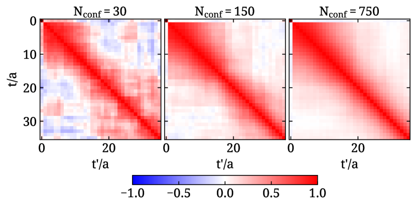
Figure 1: Correlation matrix $\bar{v}_{tt^{\prime}}$ as defined in Eq. (22) for the case of the two-point correlation function for the $\textrm{N}_{\textrm{f}}{=}2{+}1{+}1$ ensemble, cB211.072.64, for the first 35 time slices, i.e. $t,\,t^{\prime}\in[0,35]$. From left to right, we show $\bar{v}_{tt^{\prime}}$ using $N_{\textrm{conf}}{=}30$, 150, and 750 configurations.

IV Renormalization functions

The bare matrix elements of the operators defined in Eqs. (1) must be renormalized in order to obtain physical quantities. The renormalization functions ($Z$-factors) for the isovector operators considered here are multiplicative and are computed nonperturbatively. We obtain the $Z$-factors using five ensembles at different values of the pion mass, so that the chiral limit can be taken. For a proper chiral extrapolation we compute the $Z$-factors for degenerate quark flavors. For the $\textrm{N}_{\textrm{f}}{=}2$ we use the already generated gauge configurations while for the $\textrm{N}_{\textrm{f}}{=}2{+}1{+}1$ ensemble one needs to generate $\textrm{N}_{\textrm{f}}{=}4$ ensembles with the same $\beta$ value. In Table 3 we provide details on the $\textrm{N}_{\textrm{f}}{=}4$ ensembles used and the obtained $Z$-factors on each ensemble, while the results for $\textrm{N}_{\textrm{f}}{=}2$ ensembles are extensively discussed in Ref. Alexandrou et al. (2017).

We present here a summary of the methodology employed and discuss the results for the renormalization functions. We employ the Rome-Southampton method (RI^′ scheme) Martinelli et al. (1995) to compute them nonperturbatively and impose the conditions

$$Z_{q}=\frac{1}{12}{\rm Tr}\left[(S^{L}(p))^{-1}\,S^{{\rm Born}}(p)\right]\Bigr{|}_{p^{2}=\mu_{0}^{2}}\,,$$ (23)

$$Z_{q}^{-1}\,Z_{\cal O}\,\frac{1}{12}{\rm Tr}\left[\Gamma^{L}(p)\,\Gamma^{{\rm Born}-1}(p)\right]\Bigr{|}_{p^{2}=\mu_{0}^{2}} = 1\,.$$ (24)

The momentum $p$ is set to the RI^′ renormalization scale, $\mu_{0}$, $S^{{\rm Born}}$ ($\Gamma^{{\rm Born}}$) is the tree-level value of the fermion propagator (operator), and the trace is taken over spin and color indices. The momentum source method introduced in Ref. Gockeler et al. (1999) and employed in Refs. Alexandrou et al. (2011b); Alexandrou et al. (2012, 2017) for twisted mass fermions is utilized. This method offers high statistical accuracy using a small number of gauge configurations. In this work we use ten configurations to achieve a per mil accuracy. To reduce discretization effects we use democratic momenta; namely we consider the same spatial components

$$(a\,p)\equiv 2\pi\left(\frac{2n_{t}+1}{2T/a},\frac{n_{x}}{L/a},\frac{n_{x}}{L/a},\frac{n_{x}}{L/a}\right),\,n_{t}\in[2,10],\,n_{x}\in[2,5],$$ (25)

where $T/a$ ($L/a$) is the temporal (spatial) extent of the lattice in lattice units, and we restrict the momenta up to $(a\,p)^{2}{\sim}7$. An important constraint for the chosen momenta is to suppress the non-Lorentz invariant contributions ${\sum_{i}p_{i}^{4}}/{(\sum_{i}p_{i}^{2})^{2}}{<}0.3$ Constantinou et al. (2010). This is based on empirical arguments, as the aforementioned ratio appears in ${\cal O}(a^{2})$ terms in the perturbative expressions for the Green’s functions, and is expected to have a non-negligible contribution to higher orders in perturbation theory (see Refs. Alexandrou et al. (2011b); Alexandrou et al. (2012, 2017) for technical details). It is worth mentioning that we improve the nonperturbative estimates by subtracting finite lattice effects Constantinou et al. (2015); Alexandrou et al. (2017). The latter are computed to one-loop in perturbation theory and to all orders in the lattice spacing, ${\cal O}(g^{2}\,a^{\infty})$. These artifacts are present in the nonperturbative vertex functions of the fermion propagator and fermion operators under study.

To obtain the renormalization functions in the chiral limit we perform an extrapolation using a quadratic fit with respect to the pion mass of the ensemble, that is, $a^{\rm{RI}^{\prime}}(\mu_{0})+b^{\rm{RI}^{\prime}}(\mu_{0})\cdot m_{\pi}^{2}$ , where $a^{\rm{RI}^{\prime}}$ and $b^{\rm{RI}^{\prime}}$ depend on the scheme and the scale. As demonstrated in our earlier work on the renormalization functions, there is a negligible dependence on the pion mass , which is confirmed by the results on the $\textrm{N}_{\textrm{f}}{=}4$ ensembles of Table 3. Allowing $b{\neq}0$ and performing a linear extrapolation with respect to $m_{\pi}^{2}$ the data yield a slope that is compatible with zero within the small uncertainties. Selected data for all operators are shown in Table 3 on each ensemble, at a scale $(a\mu_{0})^{2}{=}2$, while the chiral extrapolation for this scale is shown in Fig. 2 for the three renormalization functions needed to renormalize $\langle x\rangle_{q}$, $\langle x\rangle_{\Delta q}$, and $\langle x\rangle_{\delta q}$, namely $Z^{\mu=\nu}_{V}$, $Z^{\mu\neq\nu}_{A}$, and $Z^{\mu\neq\nu\neq\rho\neq\mu}_{T}$ respectively. As can be seen, the pion mass dependence is negligible and within the statistical uncertainties.

In order to compare lattice values to experimental results one must convert to the same renormalization scheme and use the same reference scale $\overline{\mu}$. We employ the commonly used ${\overline{\rm MS}}$-scheme at $\overline{\mu}{=}$2 GeV. The conversion from RI^′ to the ${\overline{\rm MS}}$ scheme uses the intermediate renormalization groupiInvariant (RGI) scheme, which is scale independent. Therefore, one may use this property to relate the renormalization functions between two schemes, and in this case the RI^′ and ${\overline{\rm MS}}$:

$$Z^{\rm RGI}_{\cal O}= Z_{\cal O}^{\mbox{\scriptsize RI${}^{\prime}$}}(\mu_{0})\,\Delta Z_{\cal O}^{\mbox{\scriptsize RI${}^{\prime}$}}(\mu_{0})$$

$$= Z_{\cal O}^{\overline{\rm MS}}(2\,{\rm GeV})\,\Delta Z_{\cal O}^{\overline{\rm MS}}(2\,{\rm GeV})\,.$$ (26)

The conversion factor can be extracted from the above relation

$$C_{\cal O}^{{\rm RI}^{\prime},{\overline{\rm MS}}}(\mu_{0},2\,{\rm GeV})\equiv\frac{Z_{\cal O}^{\overline{\rm MS}}(2\,{\rm GeV})}{Z_{\cal O}^{{\rm RI}^{\prime}}(\mu_{0})}=\frac{\Delta Z_{\cal O}^{\mbox{\scriptsize RI${}^{\prime}$}}(\mu_{0})}{\Delta Z_{\cal O}^{\overline{\rm MS}}(2\,{\rm GeV})}\,.$$ (27)

The quantity $\Delta Z_{\cal O}^{\mathcal{S}}(\mu_{0})$ is expressed in terms of the $\beta$-function and the anomalous dimension $\gamma_{\cal O}^{S}\equiv\gamma^{S}$ of the operator

$$\Delta Z_{\cal O}^{\mathcal{S}}(\mu)= \left(2\beta_{0}\frac{{g^{\mathcal{S}}(\mu)}^{2}}{16\pi^{2}}\right)^{-\frac{\gamma_{0}}{2\beta_{0}}}\times$$

$$\exp\left\{\int_{0}^{g^{\mathcal{S}}(\mu)}\!\mathrm{d}g^{\prime}\left(\frac{\gamma^{\mathcal{S}}(g^{\prime})}{\beta^{\mathcal{S}}(g^{\prime})}+\frac{\gamma_{0}}{\beta_{0}\,g^{\prime}}\right)\right\}\,.$$ (28)

Table 3: Parameters and resulting $Z$-factors for the $\textrm{N}_{\textrm{f}}{=}4$ ensembles needed for the renormalization of the $\textrm{N}_{\textrm{f}}{=}2{+}1{+}1$ ensemble (cB211.072.64). The first column is the twisted bare mass parameter and the second and third columns are the pion mass in lattice and physical units respectively. The remaining columns give the $Z$-factors in the RI^′ scheme at $(a\mu_{0})^{2}{=}2$. The number in the parentheses is the statistical error.

$\beta$=1.778, $a$=0.0801(4) fm, ($L^{3}\times T$) = (24${}^{3}\times$48)
$a\mu$	$am_{\pi}$	$m_{\pi}$ [MeV]	$Z^{\mu=\nu}_{V}$	$Z^{\mu\neq\nu}_{V}$	$Z^{\mu=\nu}_{A}$	$Z^{\mu\neq\nu}_{A}$	$Z^{\mu\neq\nu=\rho}_{T}$	$Z^{\mu\neq\nu\neq\rho\neq\mu}_{T}$	$Z^{\mu=\nu\neq\rho}_{T}$
0.0060	0.14836	366(2)	1.1675(3)	1.1835(4)	1.1921(4)	1.1814(4)	1.1863(4)	1.2058(5)	1.1527(3)
0.0075	0.17287	427(2)	1.1672(2)	1.1830(2)	1.1917(2)	1.1808(2)	1.1860(3)	1.2055(2)	1.1527(2)
0.0088	0.18556	458(2)	1.1673(2)	1.1831(2)	1.1918(2)	1.1808(2)	1.1860(2)	1.2054(3)	1.1528(2)
0.0100	0.19635	485(2)	1.1676(3)	1.1836(3)	1.1922(3)	1.1815(3)	1.1866(2)	1.2061(3)	1.1530(1)
0.0115	0.21028	519(3)	1.1678(3)	1.1839(4)	1.1927(3)	1.1816(4)	1.1869(4)	1.2064(4)	1.1534(3)

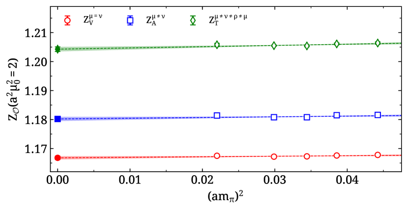
Figure 2: Example chiral extrapolation of the renormalization functions $Z_{V}^{\mu=\nu}$ (red open circles), $Z_{A}^{\mu\neq\nu}$ (blue open squares), and $Z_{T}^{\mu\neq\nu\neq\rho\neq\mu}$ (green open diamonds) for the case of $(a\mu_{0})^{2}=2$. We show with corresponding filled symbols the renormalization functions extrapolated to the chiral limit, obtained via a quadratic fit, as explained in the text.

The expressions for the one-derivative operators are known to three-loops in perturbation theory and can be found in Ref. Alexandrou et al. (2017) (and references therein).

In Fig. 3 we compare the renormalization functions in the RI^′ and ${\overline{\rm MS}}$ schemes as a function of the RI^′ renormalization scale, $\mu_{0}$. Note that the values in ${\overline{\rm MS}}$ have been evolved to 2 GeV, and from the plot we can see that the purely nonperturbative data (black points) exhibit a residual dependence on $\mu_{0}$ (the scale they were evolved from, using the appropriate expressions of Eq. (27)). This dependence is removed via two procedures:
1. the subtraction of finite-$a$ effects to ${\cal O}(g^{2}a^{\infty})$,
2. the extrapolation of $(a\mu_{0})^{2}$ to zero, using the Ansatz

$$Z_{\cal O}(a\,p)=Z_{\cal O}^{(0)}+Z_{\cal O}^{(1)}\cdot(a\,\mu_{0})^{2}\,.$$ (29)

$Z_{\cal O}^{(0)}$ corresponds to our final value of the renormalization functions for operator ${\cal O}$ (filled magenta diamonds at $(a\,\mu_{0})^{2}{=}0$), and in the above fit we consider momenta $(a\,\mu_{0})^{2}{\geq}2$ for which perturbation theory is trustworthy and lattice artifacts are still under control.

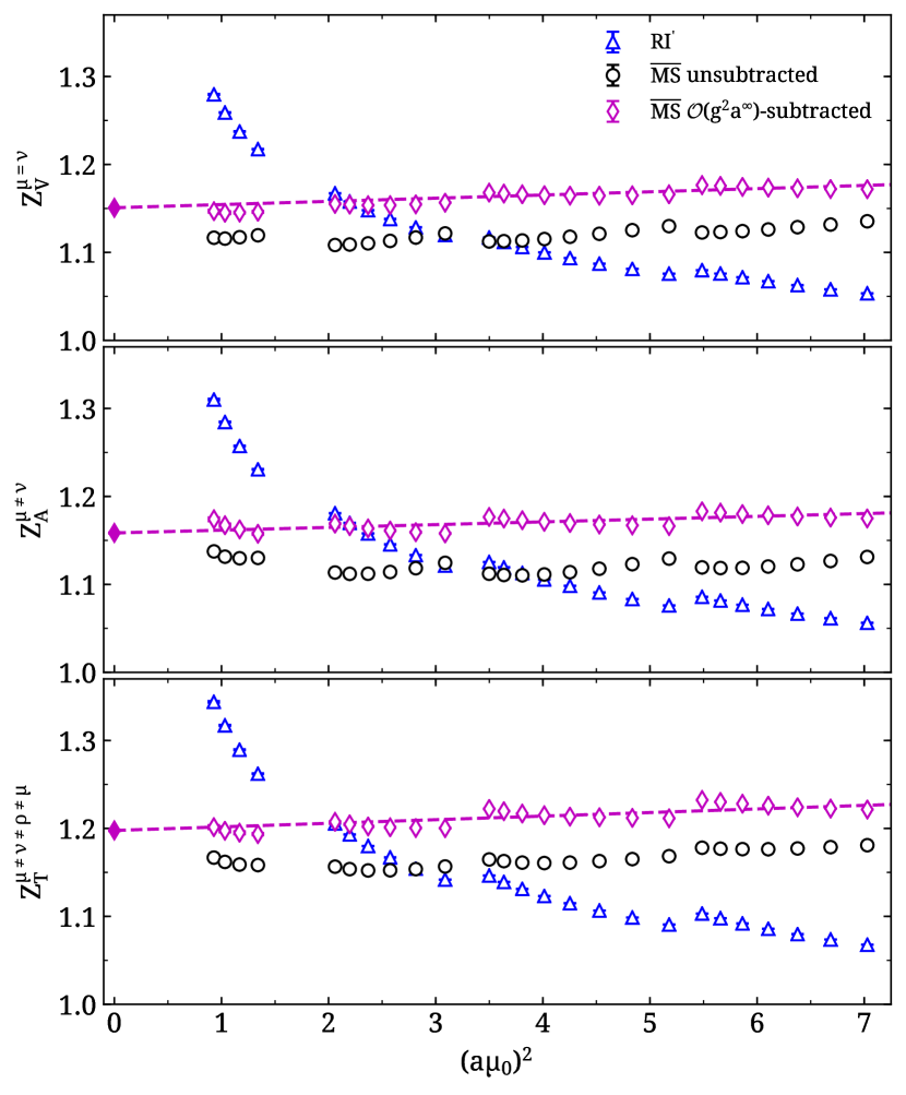
Figure 3: Chirally extrapolated results for $Z^{\mu=\nu}_{V}$ (upper plot), $Z^{\mu\neq\nu}_{A}$ (center plot), and $Z^{\mu\neq\nu\neq\rho\neq\mu}_{T}$ (lower plot), which are needed for $\langle x\rangle_{q}$, $\langle x\rangle_{\Delta q}$, and $\langle x\rangle_{\delta q}$, respectively. The data for the RI^′ scheme are shown with blue triangles, the purely nonperturbative data for the ${\overline{\rm MS}}$ scheme are shown with black circles, and the improved ${\overline{\rm MS}}$ estimates with magenta diamonds. The data are plotted as a function of the initial renormalization scale $(a\,\mu_{0})^{2}$. The dashed lines correspond to the fit of Eq. (29), and the filled magenta diamonds represent the final estimate $Z_{\cal O}^{(0)}$.

In Table 4 we report our chirally extrapolated values for the renormalization functions used in this work. The statistical and systematic uncertainties are given in the first and second sets of parentheses, respectively. The source of systematic error is related to the $(a\,\mu_{0})^{2}{\to}0$ extrapolation and it is obtained by varying the lower and higher fit ranges between $a\mu_{0}=2$ and 7 and taking the largest deviation as the systematic error. The values given in Table 4 are determined using the fit interval $(a\,\mu_{0})^{2}\,\epsilon\,[2-7]$.

Table 4: Renormalization functions for the operators used in our GFF calculation in the $\overline{\textrm{MS}}$ scheme at an energy scale of 2 GeV. The first row for the $\textrm{N}_{\textrm{f}}{=}2{+}1{+}1$ ensemble with $\beta$=1.778, and the second row for the two $\textrm{N}_{\textrm{f}}{=}2$ ensembles with $\beta$=2.1. The number in the first parentheses is the statistical error, while the number in the second parentheses corresponds to the systematic error obtained by varying the fit range in the $(a\,\mu_{0})^{2}{\to}0$ extrapolation.

Ensemble	$Z^{\mu=\nu}_{V}$	$Z^{\mu\neq\nu}_{V}$	$Z^{\mu=\nu}_{A}$	$Z^{\mu\neq\nu}_{A}$	$Z^{\mu\neq\nu=\rho}_{T}$	$Z^{\mu\neq\nu\neq\rho\neq\mu}_{T}$	$Z^{\mu=\nu\neq\rho}_{T}$
cB211.072.64	1.151(1)(4)	1.160(1)(3)	1.172(1)(4)	1.159(1)(2)	1.182(1)(2)	1.198(1)(5)	1.154(1)(9)
cA2.09.{48,64}	1.125(3)(2)	1.140(2)(1)	1.149(1)(1)	1.136(2)(20)	1.138(16)(1)	1.147(12)(5)

V Results

V.1 Zero momentum transfer

We begin by presenting our results for zero momentum transfer, which yield the isovector moments of PDFs, i.e. the momentum fraction $\langle x\rangle_{u-d}$, the helicity $\langle x\rangle_{\Delta u-\Delta d}$, and the transversity $\langle x\rangle_{\delta u-\delta d}$. In Fig. 4 we show a summary of the analyses carried out, as described in Sec. III.4, for the case of the $\textrm{N}_{\textrm{f}}{=}2{+}1{+}1$ ensemble.

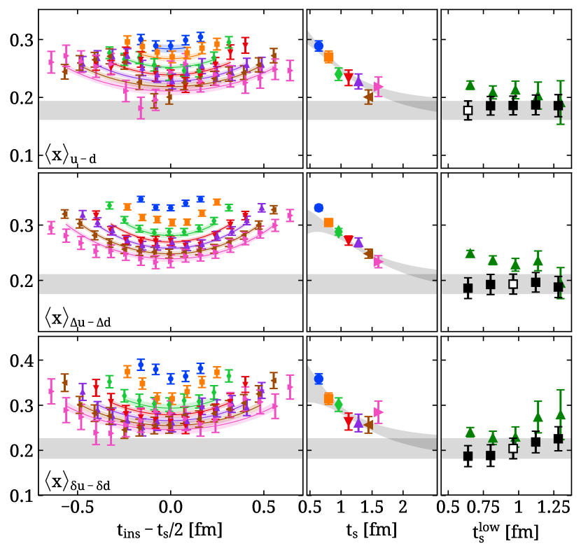
Figure 4: Results for the $\textrm{N}_{\textrm{f}}{=}2{+}1{+}1$ ensemble, cB211.072.64, for the isovector momentum fraction $\langle x\rangle_{u-d}$ (top row), the helicity moment $\langle x\rangle_{\Delta u-\Delta d}$ (middle row), and the transversity $\langle x\rangle_{\delta u-\delta d}$ (bottom row) as a function of $t_{s}$ or $t_{s}^{\textrm{low}}$ in physical units. In the left column, we show the ratio of Eq. (10) for sink-source separation $t_{s}=8a$ (blue circles), $10a$ (orange squares), $12a$ (green diamonds), $14a$ (red downwards pointing triangles), $16a$ (purple upwards pointing triangles), $18a$ (brown left pointing triangles), and $20a$ (magenta right pointing triangles), plotted against the insertion time shifted by $t_{s}/2$ so that the midpoints coincide. Data are additionally slightly shifted horizontally to ease legibility of overlapping points. The curves and corresponding bands are the result of the two-state fit. In the middle column, we show the result of the plateau fit for each sink-source separation, using the symbol notation of the left column. The band is obtained from the two-state fit parameters, as explained in the text. The right column shows the result of the summation method (green triangles) and the two-state fit method (black squares) as a function of the lower value $t_{s}^{\rm low}$ included in the fit. The open black square shows the selected value and the horizontal band spanning all three columns is the associated error band.

In the first column of Fig. 4, we plot the ratios of Eq. (10) for the three moments. In the central column, we plot the values obtained from plateau fits to the ratio as a function of the sink-source separation $t_{s}$. We show the plateaus obtained taking the insertion fit range: $t_{\textrm{ins}}\in[\tau_{\textrm{plat}},t_{s}-\tau_{\textrm{plat}}]$ choosing $\tau_{\textrm{plat}}$ such that when it is increased, the values obtained for the plateau fit do not change for each $t_{s}$. We find $\tau_{\textrm{plat}}=7a$ satisfies this criterion, and for the separations for which $t_{s}<14a$ we plot the value of the ratio at the midpoint, i.e. for $t_{\textrm{ins}}=t_{s}/2$, in the central column of Fig. 4.

As explained for the two-state fit we first fit the two-point function at zero momentum. The values we extract for $m_{N}$ and $m_{N}^{*}$ remain unchanged within errors if we include a second excited state, i.e. if we perform a three-state fit. While in the spectral decomposition of the two-point correlation function, the energy state above the nucleon should include a pion-nucleon with relative momentum, it is noteworthy that for all ensembles we find a value for $m_{N}^{*}$ that is consistent to the mass of the Roper rather than a multiparticle state, as shown in Table 5.

Table 5: Values of the excited state mass $m_{N}^{*}$, in GeV, as extracted from the two-state (first row of results) and three-state (second row of results) fits to the two-point functions of the three ensembles analyzed in this work.

	cB211.072.64		cA2.09.48		cA2.09.64
Two-state:	1.	43(7)	1.	59(6)	1.	45(11)
Three-state:	1.	38(12)	1.	44(15)	1.	15(16)

The results obtained using the summation and two-state fit methods are shown in the right column of Fig. 4, as a function of the smallest sink-source separation used in the fit $t_{s}^{\textrm{low}}$. For the two-state fit method, we choose the fit range for the two-point function by requiring the ground state mass extracted with the two-exponential ansatz of Eq. (14) to agree with that obtained from a constant fit to the effective mass, within half the error of the latter. This analysis yields $t_{s}\in[8a,\,35a]$ in the case of the $\textrm{N}_{\textrm{f}}{=}2{+}1{+}1$ ensemble and this is used throughout. Furthermore, we find that taking $t_{\textrm{ins}}\in[\tau,\,t_{s}-\tau]$ for $\tau\geq 3a$ in the two-state fit yields consistent results, and thus we fix $\tau{=}3a$.

From the right column of Fig. 4, we see that in general the two-state fit results are stable for all $t_{s}^{\textrm{low}}$ values, with the summation method converging as $t_{s}^{\textrm{low}}$ is increased. The bands in the left column of Fig. 4 show the ratio of Eq. (10) when using the parameters of the two-state fit to reproduce the two- and three-point functions, namely Eqs. (14) and (15). We see that in all cases, the predicted bands reproduce the data well.

The band in the central column of Fig. 4 is not a fit to the data; it is drawn using the parameters obtained from the two-state fit as a function of continuous values for $t_{s}$ and taking $t_{\textrm{ins}}=t_{s}/2$. The left and central columns show that the data are reproduced well with the two-state fit ansatz. Furthermore, the band drawn in the central column reveals that sink-source separations beyond $\approx 2$ fm are required to obtain plateaus that would sufficiently suppress the first excited state and therefore yield agreement between the plateau and two-state fit methods. Such a separation would not be feasible with currently available computational resources. Indeed, between our smallest and largest separations of 0.64 fm and 1.6 fm respectively, we increase statistics by 64$\times$ (see Table 2) while errors increase by $\sim$2.5$\times$, indicating that to obtain at $\sim 2$ fm the same error as that obtained at 1.6 fm we would require ${\cal O}(100)$ more statistics. We will therefore quote the result of the two-state fit method as our final result, shown by the horizontal band spanning all columns in Fig. 4.

To choose the $t_{s}^{\textrm{low}}$ of the two-state fit for quoting our final result, we will demand that this agrees with the converged value of the summation method. For $\langle x\rangle_{u-d}$ the two-state fit result with $t_{s}^{\textrm{low}}{=}8a$ agrees with the result of the summation method for $t_{s}^{\textrm{low}}>$1 fm. We therefore take the two-state fit result with $t_{s}^{\textrm{low}}{=}8a$ as our final value for the momentum fraction. For the helicity $\langle x\rangle_{\Delta u-\Delta d}$ and tensor charge $\langle x\rangle_{\delta u-\delta d}$, as can be seen, we need to increase $t_{s}^{\rm low}$ further to achieve agreement with the summation method. We therefore take the value when fitting from $t_{s}^{\textrm{low}}{=}12a$ as our final result.

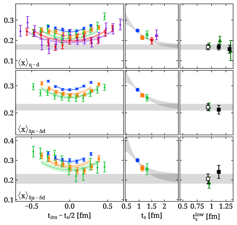
Figure 5: Results for the small $\textrm{N}_{\textrm{f}}{=}2$ ensemble, cA2.09.48. In the left column, we show the ratio of Eq. (10) for sink-source separation $t_{s}{=}10a$ (blue circles), $12a$ (orange squares), $14a$ (green diamonds), $16a$ (red downwards pointing triangles), and $18a$ (purple upwards pointing triangles). The rest of the notation is as in Fig. 4.

The same analysis is carried out for the small and large $\textrm{N}_{\textrm{f}}{=}2$ ensembles, shown in Figs. 5 and 6, respectively. The analysis of the $\textrm{N}_{\textrm{f}}{=}2{+}1{+}1$ ensemble, for which we use seven values of $t_{s}$ with increased statistics, has clearly revealed that excited state effects die out slowly and that one needs to go to larger values of $t_{s}$ Bar (2019) keeping statistical errors small to see clear convergence as also demonstrated in Ref. von Hippel et al. (2017). With this hindsight, we reanalyze the $\textrm{N}_{\textrm{f}}{=}2$ ensembles. For determining the fit ranges of the two-point function we use the same criteria as for the $\textrm{N}_{\textrm{f}}{=}2{+}1{+}1$ ensemble. We find that $t_{s}\in[6a,\,24a]$ for the small $\textrm{N}_{\textrm{f}}{=}2$ ensemble and $t_{s}\in[5a,\,24a]$ for the large $\textrm{N}_{\textrm{f}}{=}2$ ensemble satisfy the agreement between the values extracted from one-state (plateau) and two-state fits. While for the $\textrm{N}_{\textrm{f}}{=}2{+}1{+}1$ and small $\textrm{N}_{\textrm{f}}{=}2$ ensembles we have increased statistics for the two-point functions used in the two-state fit method, for the large $\textrm{N}_{\textrm{f}}{=}2$ ensemble we are limited to the same statistics for two-point functions as those for the three-point function. The reason is that for the latter ensemble we did not compute disconnected contributions. This also explains why the lower fit range for the large $\textrm{N}_{\textrm{f}}{=}2$ ensemble is smaller as compared to the small $\textrm{N}_{\textrm{f}}{=}2$ ensemble, since the two-point correlator has lower precision. In the case of the three-point function, for both these ensembles, in general only three sink-source separations are available, which allow for only a single point for the summation method and two points for the two-state fit method. The unpolarized projector for the case of the small $\textrm{N}_{\textrm{f}}{=}2$ ensemble is the only exception, namely for this case we obtain $\langle x\rangle_{u-d}$, for two additional separations.

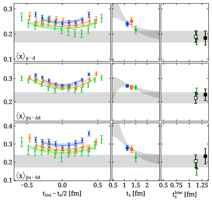
Figure 6: Results for the large $\textrm{N}_{\textrm{f}}{=}2$ ensemble, cA2.09.64. The left column shows the ratio of Eq. (10) for sink-source separation $t_{s}{=}12a$ (blue circles), $14a$ (orange squares), and $16a$ (green diamonds). The rest of the notation is as in Fig. 4.

From Figs. 5 and 6 we observe a curvature in the ratio data similar to that of the $\textrm{N}_{\textrm{f}}{=}2{+}1{+}1$ ensemble. For the plateau fits shown in the central columns, we use $\tau_{\textrm{plat}}=5a$ for both ensembles, determined using the same criterion as for the $\textrm{N}_{\textrm{f}}{=}2{+}1{+}1$ case. Comparing two-state fit and summation methods, we note that at the smallest $t_{s}^{\textrm{low}}$ available for these two ensembles, which is around $\sim$1 fm, we see agreement between two-state and summation methods. For all three ensembles, therefore, the summation method at around $t_{s}^{\textrm{low}}\simeq$1 fm converges to the two-state fit result within errors. We take the two-state fit result as our final value for these two ensembles. Our final results for the three moments are given in Table 6.

Table 6: Results for the three isovector moments from the three ensembles analyzed in this work. The results are obtained from the two-state fit as explained in the text.

Ensemble	$\langle x\rangle_{u-d}$	$\langle x\rangle_{\Delta u-\Delta d}$	$\langle x\rangle_{\delta u-\delta d}$
cB211.072.64	0.178(16)	0.193(18)	0.204(23)
cA2.09.48	0.167(13)	0.221(12)	0.206(25)
cA2.09.64	0.189(23)	0.217(24)	0.205(35)

Comparing the three moments between the three ensembles, we see in general that these agree within our statistical errors, an exception being $\langle x\rangle_{\Delta u-\Delta d}$ for $\textrm{N}_{\textrm{f}}{=}2{+}1{+}1$ and the $\textrm{N}_{\textrm{f}}{=}2$ ensembles, where agreement is within 1.5$\sigma$ of the former.

Comparing the results obtained using the two $\textrm{N}_{\textrm{f}}{=}2$ ensembles, which differ only in their volume, with $m_{\pi}L$=2.98 to 3.97, respectively reveals no finite volume effects within our statistical errors for all three moments. The $\textrm{N}_{\textrm{f}}{=}2{+}1{+}1$ ensemble has $m_{\pi}L$=3.62 (see Table 1), which is between the two volumes with $\textrm{N}_{\textrm{f}}{=}2$ and thus we also expect that volume effects are also within the statistical errors for this ensemble as well. The $\textrm{N}_{\textrm{f}}{=}2{+}1{+}1$ ensemble has a smaller lattice spacing and includes the strange and charm quarks in the sea. We find that the moments obtained using the $\textrm{N}_{\textrm{f}}{=}2{+}1{+}1$ ensemble and the two $\textrm{N}_{\textrm{f}}{=}2$ ensembles are in agreement. This suggests that unquenching effects and cutoff effects for these quantities, at least within the range of these two lattice spacings, are also smaller than our statistical uncertainties.

V.2 Finite momentum transfer

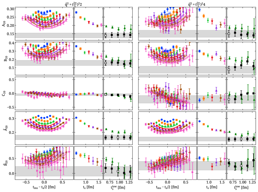
Figure 7: Results for the vector and axial GFFs for the $\textrm{N}_{\textrm{f}}{=}2{+}1{+}1$ ensemble, cB211.072.64 for two representative $\vec{q}^{2}$ values corresponding to $Q^{2}=0.114$ GeV² (left) and 0.222 GeV² (right). The first three rows show results for the three vector GFFs, namely $A_{20}$, $B_{20}$, and $C_{20}$, and the last two rows for the two axial GFFs $\tilde{A}_{20}$ and $\tilde{B}_{20}$. For each of the two values of $Q^{2}$ shown, we use the same notation as for the $Q^{2}=0$ case of Fig. 4, namely showing the ratio obtained as explained in the text (left columns), the result of fitting the plateau in the single step approach (central columns), and the results from two-state fits and summation method (right columns).

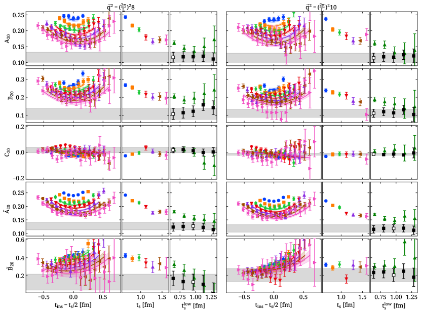
Figure 8: The same as in Fig. 7 but for $Q^{2}{=}0.421$ GeV² (left) and $Q^{2}{=}0.514$ GeV² (right).

To obtain the GFFs we perform, for each value of the momentum transfer squared, a similar analysis as for the moments. This analysis is summarized in Figs. 7 and 8 for the $\textrm{N}_{\textrm{f}}{=}2{+}1{+}1$ lattice for four representative values of the momentum transfer squared. We note that for the ratios of Figs. 7 and 8 we plot, for each value of $Q^{2}$ and $t_{s}$, the quantity: $V^{\dagger}\Sigma^{-1}U^{\dagger}R(\Gamma;\vec{q};t_{s},t_{\textrm{ins}})$, where $R$ is the ratio of Eq. (10) and $U$, $\Sigma$, and $V$ are obtained from the SVD of the kinematic matrix $\mathcal{G}$ defined in Eq. (13). This is done for the purposes of presenting our results in a similar way to that of the moments in Fig. 4, whereas in the analysis, to extract the result of the plateau from the single step approach, we fit the combination $U^{\dagger}R$. As in the case of the moments, we observe non-negligible excited state effects in the ratios as we increase $t_{s}$. The two-state fit results are stable as we increase $t_{s}^{\textrm{low}}$ and the summation method converges to the two-state fit value for $t_{s}^{\textrm{low}}\simeq$ 1 fm. We therefore use the two-state fit to extract our final values for the GFFs for all $Q^{2}$ using the same fit parameters as for the moments.

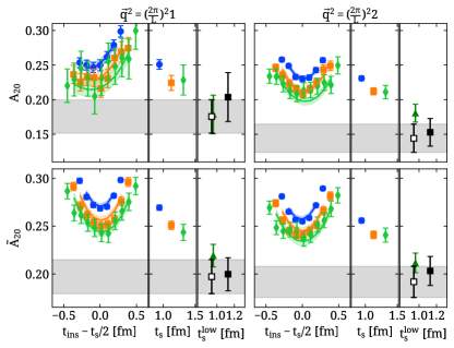
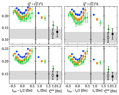
Figure 9: Results for the dominant vector (first row) and axial (second row) GFFs for the small $\textrm{N}_{\textrm{f}}{=}2$ ensemble, cA2.09.48 for four representative $Q^{2}$ values. For each value of $Q^{2}$, we use the same notation as for the $Q^{2}=0$ case of Fig. 5.

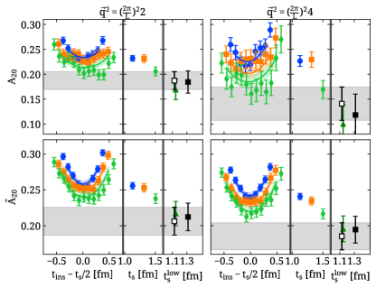
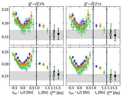
Figure 10: Results for the dominant vector (first row) and axial (second row) GFFs for the large $\textrm{N}_{\textrm{f}}{=}2$ ensemble, cA2.09.64 for four representative $Q^{2}$ values. For each value of $Q^{2}$, we use the same notation as for the $Q^{2}=0$ case of Fig. 6.

The same procedure is followed for the small and large $\textrm{N}_{\textrm{f}}{=}2$ ensembles shown in Figs. 9 and 10 respectively, in which we show the dominant vector and axial GFFs, namely $A_{20}$ and $\tilde{A}_{20}$. We show four representative momentum transfer values for the two ensembles, chosen such that they are approximately equal in physical units. Note that for extracting the vector GFFs we require all four projectors (see Appendix A), which means that for the small $\textrm{N}_{\textrm{f}}{=}2$ ensemble we are restricted to three sink-source separations for $Q^{2}{>}0$.

From Figs. 9 and 10, we see that summation and two-state fit methods yield consistent results for the $Q^{2}$ values shown. This is confirmed for all $Q^{2}$ values, and for the subdominant vector and axial GFFs, namely $B_{20}$, $\tilde{B}_{20}$ and $C_{20}$.

The availability of the two $\textrm{N}_{\textrm{f}}{=}2$ ensembles that differ only in their volumes allows us to assess finite volume effects. A comparison between the results obtained using these two ensembles is shown in Fig. 11, for all five GFFs using our final values extracted from two-state fits. As in the case of the moments shown in Table 6, comparing these two ensembles reveals no finite volume effects within the achieved statistical precision. The small discrepancies seen for $A_{20}$ at some values of the momentum are well within the allowed statistical fluctuations. We stress that these results are extracted taking into account correlations. Were we to ignore the correlations among different $t_{s}$ the errors increase and no disagreement is observed.

In Fig. 12 we show the five GFFs for the $\textrm{N}_{\textrm{f}}{=}2{+}1{+}1$ ensemble obtained from the two-state fit method. We note that $C_{20}$ is found to be consistently zero for all $Q^{2}$, in agreement with previous lattice results for this quantity Alexandrou et al. (2013); Bali et al. (2018).

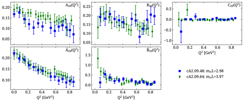
Figure 11: Comparison of the vector (top row) and axial (bottom row) GFFs between the two $\textrm{N}_{\textrm{f}}{=}2$ ensembles cA2.09.64 (green diamonds) and cA2.09.48 (blue squares) which differ only in the volume, namely with $m_{\pi}L$=3.97 and 2.98 respectively. We show results obtained using two-state fits.

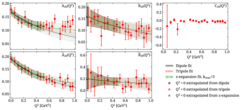
Figure 12: Results for the vector (top row) and axial (bottom row) GFFs for the $\textrm{N}_{\textrm{f}}{=}2{+}1{+}1$ ensemble, cB211.072.64, obtained using the two-state fit method. Dipole (solid black curves), tripole (dashed red curves), and $z$-expansion (dot-dashed green curves) fits are shown using $Q^{2}\leq 0.5$ GeV², while the dotted curves extend the fits beyond $Q^{2}$=0.5 GeV². For $B_{20}$ and $\tilde{B}_{20}$ we also show the value at $Q^{2}$=0 extracted from the dipole (open black asterisk), tripole (open red asterisk), and $z$-expansion (open green asterisk) fits, the latter two shifted slightly to improve legibility.

For the $A_{20},B_{20},\tilde{A}_{20}$ and $\tilde{B}_{20}$ with nonzero signal, we perform fits to the form

$$G(Q^{2})=\frac{G(0)}{(1+Q^{2}/M^{2})^{n}},$$ (30)

as well as using the so-called $z$-expansion Hill and Paz (2010)

$$G(Q^{2})=\sum_{k=0}^{k_{\textrm{max}}}a_{k}z^{k},$$ (31)

with:

$$z=\frac{\sqrt{t_{\textrm{cut}}+Q^{2}}-\sqrt{t_{\textrm{cut}}}}{\sqrt{t_{\textrm{cut}}+Q^{2}}+\sqrt{t_{\textrm{cut}}}}.$$ (32)

The dipole form, obtained by setting $n=2$ in Eq. (30), is supported by model considerations as e.g. in the quark-soliton model in the large $N_{C}$ limit for $Q^{2}<1$ GeV² Goeke et al. (2007). Fitting to our data for $Q^{2}\leq 0.5$ GeV² allowing $G(0)$ and $M$ to vary, we obtain the results shown in Table 7, where we also include the $\chi^{2}$ per degrees of freedom (d.o.f) which indicates that this Ansatz models our data well. In Fig. 12 we show the resulting fit to the data with the solid line. For the case of the GFFs $B_{20}$ and $\tilde{B}_{20}$ we also consider the tripole form by setting $n=3$ in Eq. (30). Such a form has been shown to satisfy certain constraints in the energy and pressure distributions inside the nucleon Lorcé et al. (2019). The resulting tripole fit (dashed line in Fig. 12) is fully consistent with the dipole yielding similar values for $B_{20}(0)$ and $\tilde{B}_{20}(0)$ as the dipole form, as can be seen in Table 7.

The $z$-expansion provides for a model-independent Ansatz and has been originally developed for fitting electromagnetic Hill and Paz (2010) and axial Bhattacharya et al. (2011) form factors. In Eq. (32), we use $t_{\textrm{cut}}=(4m_{\pi})^{2}$ and $(3m_{\pi})^{2}$ for the vector and axial cases respectively, and fit varying the parameters $a_{k}$ studying their convergence as we increase $k_{\textrm{max}}$. Without loss of generality, demanding that the GFFs are zero as $Q^{2}\rightarrow\infty$ constrains one parameter, which we implement by setting $a_{k_{\textrm{max}}}=-\sum_{k=0}^{k_{\textrm{max}}-1}a_{k}$. Furthermore, in the fit we use priors for the parameters $a_{k}$ for $1<k<k_{\textrm{max}}$. The prior width is determined as $5\max(a_{0},a_{1})$, as obtained from the fit using $k_{\textrm{max}}$=2. As we increase $k_{\textrm{max}}$, we find that the parameters $a_{0}$ and $a_{1}$ do not change after $k_{\textrm{max}}=3$, for which we quote the fit parameters in Table 7. To compare with the dipole fit, for the $z$-expansion we quote: $M=\sqrt{-8a_{0}t_{\textrm{cut}}/a_{1}}$, which is the dipole mass that yields the same slope as the $z$-expansion for the GFF at $Q^{2}=0$.

Table 7: The parameters extracted from fitting $A_{20},B_{20},\tilde{A}_{20}$ and $\tilde{B}_{20}$ to the dipole form ($n=2$ in Eq. (30)) and the $z$-expansion (Eq. (31)) and $B_{20}$ and $\tilde{B}_{20}$ to the tripole form ($n=3$ in Eq. (30)). We use $Q^{2}\leq 0.5$ GeV². For the $z$-expansion we show results for $k_{\textrm{max}}=3$, with $G(0)=a_{0}$ and $M=\sqrt{-\frac{8a_{0}t_{\textrm{cut}}}{a_{1}}}$.

	$G(0)$	$M$ [GeV]	$\chi^{2}$/d.o.f
	Dipole
${A}_{20}$	0.167(13)	1.41(27)	0.4
${B}_{20}$	0.159(41)	1.64(72)	0.5
$\tilde{A}_{20}$	0.190(13)	1.32(17)	0.1
$\tilde{B}_{20}$	0.20(17)	1.7(2.8)	0.2
	Tripole
${B}_{20}$	0.158(40)	2.05(88)	0.5
$\tilde{B}_{20}$	0.20(17)	2.1(3.4)	0.2
	$z$-expansion ($k_{\textrm{max}}=3$)
${A}_{20}$	0.174(14)	1.03(28)	0.2
${B}_{20}$	0.163(45)	1.36(90)	0.4
$\tilde{A}_{20}$	0.195(15)	1.08(47)	0.1
$\tilde{B}_{20}$	0.21(21)	1.2(2.1)	0.2

V.3 Comparison of results with other studies

We compare our results with phenomenology as well as other lattice studies with physical or near-physical pion masses.

The isovector momentum fraction $\langle x\rangle_{u-d}$ has been extensively calculated in lattice QCD at pion masses larger than its physical value, and a review of results can be found in Ref. Lin et al. (2018). Recent results include results using CLS N_f=2+1 clover improved Wilson fermions from the Mainz group Harris et al. (2019), as well as from two collaborations at physical or near-physical pion mass: RQCD, using $\textrm{N}_{\textrm{f}}{=}2$ clover improved Wilson fermions Bali et al. (2018) and LHPC Green et al. (2014) using N_f=2+1 HEX-smeared clover improved fermions. RQCD analyzed 11 ensembles among which one that has near-physical pion mass of 150 MeV, a lattice volume of $64^{3}\times 64$ and $a=0.071$ fm. The authors analyzed three sink-source time separations for this ensemble within $t_{s}\in[0.6,1.1]$ fm, and conclude that suppressing the excited states would require additional separations that agrees with our findings. They, therefore, restrict themselves to showing results using a single separation at $15a\simeq 1.1$ fm, which is too small to control excited states. Their value of 0.213(11)(04) is compatible with the one we find at the similar sink-source time separation of 1.12 fm, namely 0.232(11), that clearly overestimates the momentum fraction extracted from larger values of $t_{s}$ and from the two-state fit. We thus do not include this result in our comparison. LHPC analyzed one ensemble with pion mass of $m_{\pi}$=149 MeV, a lattice volume of 48${}^{3}\times$48 and $a=0.116$ fm. The summation method is used to obtain their final value from three sink-source separations with values 0.9, 1.2, and 1.4 fm .

Results for $\langle x\rangle_{u-d}$ are shown in Fig. 13 where we include the phenomenological values extracted from global fits to PDF experimental data from Refs. Ball et al. (2017); Dulat et al. (2016); Harland-Lang et al. (2015); Alekhin, S. and Blümlein, J. and Moch, S. and Placakyte, R. (2017); Accardi et al. (2016); Abramowicz et al. (2015). Results from our three ensembles are consistent with each other, indicating no detectable lattice artifacts within their precision. Results for the $\textrm{N}_{\textrm{f}}{=}2{+}1{+}1$ ensemble are obtained using more time separations allowing for a more rigorous assessment of exited state effects compared to the other two ensembles. We thus take the value extracted from the $\textrm{N}_{\textrm{f}}{=}2{+}1{+}1$ ensemble to compare with phenomenology. We observe agreement with two of the phenomenological extractions shown in Fig. 13, with the remaining within 1.5$\sigma$ of our value.

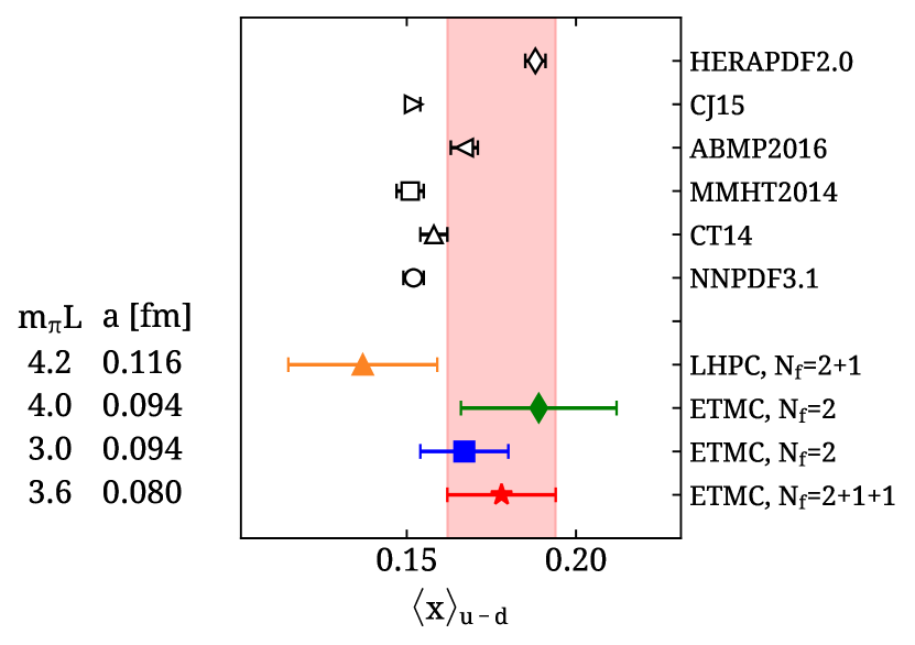
Figure 13: $\langle x\rangle_{u-d}$ from the three ensembles studied in this work, namely the $\textrm{N}_{\textrm{f}}{=}2{+}1{+}1$ (red star), small $\textrm{N}_{\textrm{f}}{=}2$ (blue square), and large $\textrm{N}_{\textrm{f}}{=}2$ (green diamond) ensembles. We compare to lattice results from Ref. Green et al. (2014) (orange triangle). We also show results from global fits to PDF experimental data with the open symbols, namely NNPDF3.1 Ball et al. (2017) (circle), CT14 Dulat et al. (2016) (triangle), MMHT2014 Harland-Lang et al. (2015) (square), ABMP2016 Alekhin, S. and Blümlein, J. and Moch, S. and Placakyte, R. (2017)(left-pointing triangle), CJ15 Accardi et al. (2016) (right-pointing triangle), and HERAPDF2.0 Abramowicz et al. (2015) (diamonds).

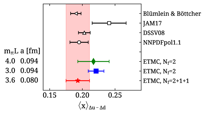
Figure 14: $\langle x\rangle_{\Delta u-\Delta d}$ from the three ensembles studied in this work with the notation of Fig. 13. We compare to results from global fits to polarized PDF experimental data with the open symbols, namely from Ref. Blümlein, Johannes and Böttcher, Helmut (2010) (left-pointing triangle), NNPDFpol1.1 Nocera et al. (2014) (circle), DSSV08 de Florian et al. (2009) (triangle), and JAM17 Ethier et al. (2017) (square).

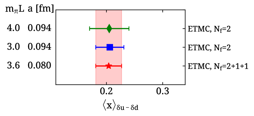
Figure 15: $\langle x\rangle_{\delta u-\delta d}$ from the three ensembles studied in this work with the notation of Fig. 13.

For $\langle x\rangle_{\Delta u-\Delta d}$ our results are compared in Fig. 14 to phenomenological results from Refs. Ethier et al. (2017); Nocera et al. (2014); Blümlein, Johannes and Böttcher, Helmut (2010); de Florian et al. (2009). As can be seen, our value is in good agreement with these phenomenological determinations and in particular with the value found in Ref. Blümlein, Johannes and Böttcher, Helmut (2010). The results for $\langle x\rangle_{\delta u-\delta d}$ are shown in Fig. 15. No phenomenological nor other lattice QCD results at the physical point are available for the tensor moment and thus the current work provides a valuable prediction. We note that for the helicity and tensor moments only three sink-source time separations are available in the case of the two $\textrm{N}_{\textrm{f}}{=}2$ ensembles. This restricts the two-state analysis and thus we consider the result of the $\textrm{N}_{\textrm{f}}{=}2{+}1{+}1$ ensemble as the most reliable. As already mentioned, the two $\textrm{N}_{\textrm{f}}{=}2$ ensembles show no detectable volume dependence for these quantities indicating that volume effects are negligible as compared to the current accuracy obtained from the analysis using the $\textrm{N}_{\textrm{f}}{=}2{+}1{+}1$ ensemble.

VI Conclusions

The isovector momentum fraction, helicity moment, and transversity of the nucleon are extracted using lattice QCD simulations produced with physical values of the quark masses. For the $\textrm{N}_{\textrm{f}}{=}2{+}1{+}1$ ensemble cB211.072.64, seven sink-source separations are analyzed from 0.6 fm to 1.6 fm, allowing for the most thorough study of excited states to date for these quantities directly at the physical pion mass. The isovector unpolarized and helicity GFFs are also extracted for the first time directly at the physical point. The study reveals that both for $Q^{2}=0$ as well as for $Q^{2}>0$, the convergence of these quantities to the ground state is slow. For values of the sink-source time separation $t_{s}<2$ fm a two-state fit analysis yields stable results and agrees with the values extracted from the summation method when including separations larger than $\sim$1 fm. We therefore, take the results from the two-state fit when confirmed with the summation method as our final values. The results for the GFFs are provided in Tables 8, 9, and 10 of Appendix C and in Table 6 for the moments. For the case of the small $\textrm{N}_{\textrm{f}}{=}2$ ensemble, the current results for the moments are an update to those of Ref. Abdel-Rehim et al. (2015), which are included for comparison in Appendix D. The $\textrm{N}_{\textrm{f}}{=}2{+}1{+}1$ ensemble includes dynamical strange and charm quarks in addition to the light quarks thus providing a full description of the QCD vacuum. In addition, the seven sink-source separations are analyzed to high accuracy allowing for a robust analysis of excited states. We thus consider the results extracted from the $\textrm{N}_{\textrm{f}}{=}2{+}1{+}1$ ensemble as the best prediction of these quantities. We thus quote as our final results the values obtained from the analysis of the $\textrm{N}_{\textrm{f}}{=}2{+}1{+}1$ ensemble. We find for the moments:

$$\langle x\rangle_{u-d} =0.178(16),$$

$$\langle x\rangle_{\Delta u-\Delta d} =0.193(18),$$

$$\langle x\rangle_{\delta u-\delta d} =0.204(23),$$ (33)

where we quote the values extracted directly from the nucleon matrix element at zero momentum. The values for the unpolarized and helicity moments agree with a subset of the phenomenological results. The helicity and transversity moments $\langle x\rangle_{\Delta q}$ and $\langle x\rangle_{\delta q}$, are shown to be related to longitudinal and transverse spin-orbit correlations, respectively Lorcé (2014); Bhoonah and Lorcé (2017) and are interpreted as the parity and chiral partners of Ji’s relation for angular momentum.

Fits of the GFFs yield the results provided in Table 7. From these fits we obtain $B_{20}(0)$, which is related to the proton spin via Ji’s sum rule Ji (1997). Using the values for $\textrm{N}_{\textrm{f}}{=}2{+}1{+}1$ obtained by fits to the dipole form, we obtain:

$$J^{u-d}=\frac{1}{2}[A^{u-d}_{20}(0)+B^{u-d}_{20}(0)]=0.168(22)(02)$$ (34)

for the isovector contribution of the up and down quarks to the proton spin, where the first error is statistical and the second a systematic obtained as the difference in $B_{20}$ between the extraction using the dipole form and the $z$-expansion.

A next step in this study will be the inclusion of disconnected contributions in order to calculate the isoscalar and gluonic quantities. This would allow for complete flavor decomposition of the GFFs and for calculating the spin and momentum carried by quarks and gluons in the proton.

Appendix A Expressions for generalized form factors

The following expressions are provided in Euclidean space. We suppress the $Q^{2}=-q^{2}$ argument of the generalized form factors, $E_{N}$ is the nucleon energy for three-momentum $\vec{q}$, the kinematic factor $\mathcal{K}=\sqrt{2m_{N}^{2}/[E_{N}(E_{N}+m_{N})]}$ and Latin indices ($k$, $n$, and $j$) take values 1, 2, and 3 with $k\neq j$ while $\rho$ takes values 1, 2, 3, and 4.

A.1 Vector operator

$$\Pi_{V}^{00}(\Gamma^{0},\vec{q})= A_{20}\,\mathcal{K}\,\left(-\frac{3\,E_{N}}{8}-\frac{E_{N}^{2}}{4\,m_{N}}-\,\frac{m_{N}}{8}\right)+B_{20}\,\mathcal{K}\,\left(-\,\frac{E_{N}}{8}+\,\frac{E_{N}^{3}}{8\,m_{N}^{2}}+\frac{E_{N}^{2}}{16\,m_{N}}-\frac{m_{N}}{16}\right)$$

$$+ C_{20}\,\mathcal{K}\,\left(\,\frac{E_{N}}{2}-\frac{E_{N}^{3}}{2\,m_{N}^{2}}+\frac{E_{N}^{2}}{4\,m_{N}}-\frac{m_{N}}{4}\right),$$ (35)

$$\Pi_{V}^{00}(\Gamma^{n},\vec{q})= 0,$$ (36)

$$\Pi_{V}^{kk}(\Gamma^{0},\vec{q})= A_{20}\,\mathcal{K}\,\left(\frac{E_{N}}{8}+\frac{m_{N}}{8}+\frac{q_{k}^{2}}{4\,m_{N}}\right)+B_{20}\,\mathcal{K}\,\left(-\frac{E_{N}^{2}}{16\,m_{N}}+\frac{m_{N}}{16}-\frac{q_{k}^{2}\,E_{N}}{8\,m_{N}^{2}}+\frac{q_{k}^{2}}{8\,m_{N}}\right)$$

$$+ C_{20}\,\mathcal{K}\,\left(-\frac{E_{N}^{2}}{4\,m_{N}}+\frac{m_{N}}{4}+\frac{q_{k}^{2}\,E_{N}}{2\,m_{N}^{2}}+\frac{q_{k}^{2}}{2\,m_{N}}\right),$$ (37)

$$\Pi_{V}^{kk}(\Gamma^{n},\vec{q})= A_{20}\,\mathcal{K}\,\left(-i\,\frac{\epsilon_{k\,n\,0\,\rho}\,q_{k}\,q_{\rho}}{4\,m_{N}}\right)+B_{20}\,\mathcal{K}\,\left(-i\,\frac{\epsilon_{k\,n\,0\,\rho}\,q_{k}\,q_{\rho}}{4\,m_{N}}\right),$$ (38)

$$\Pi_{V}^{k0}(\Gamma^{0},\vec{q})= A_{20}\,\mathcal{K}\,\left(-i\,\frac{q_{k}}{4}-i\,\frac{q_{k}\,E_{N}}{4\,m_{N}}\right)+B_{20}\,\mathcal{K}\,\left(-i\,\frac{q_{k}}{8}+i\,\frac{q_{k}\,E_{N}^{2}}{8\,m_{N}^{2}}\right)+C_{20}\,\mathcal{K}\,\left(i\,\frac{q_{k}}{2}-i\,\frac{q_{k}\,E_{N}^{2}}{2\,m_{N}^{2}}\right),$$ (39)

$$\Pi_{V}^{k0}(\Gamma^{n},\vec{q})= A_{20}\,\mathcal{K}\,\left(\,-\epsilon_{k\,n\,0\,\rho}\,\left(\frac{q_{\rho}}{8}+\frac{q_{\rho}\,E_{N}}{8\,m_{N}}\right)\right)+B_{20}\,\mathcal{K}\,\left(\,-\epsilon_{k\,n\,0\,\rho}\,\left(\frac{q_{\rho}}{8}+\frac{q_{\rho}\,E_{N}}{8\,m_{N}}\right)\right)$$ (40)

$$\Pi_{V}^{kj}(\Gamma^{0},\vec{q})= A_{20}\,\mathcal{K}\,\frac{q_{k}\,q_{j}}{4\,m_{N}}+B_{20}\,\mathcal{K}\,\left(-\frac{q_{k}\,q_{j}\,E_{N}}{8\,m_{N}^{2}}+\frac{q_{k}\,q_{j}}{8\,m_{N}}\right)+C_{20}\,\mathcal{K}\,\left(\frac{q_{k}\,q_{j}\,E_{N}}{2\,m_{N}^{2}}+\frac{q_{k}\,q_{j}}{2\,m_{N}}\right),$$ (41)

$$\Pi_{V}^{kj}(\Gamma^{n},\vec{q})= A_{20}\,\mathcal{K}\,\left(-i\,\frac{\epsilon_{k\,n\,0\,\rho}\,q_{j}\,q_{\rho}}{8\,m_{N}}-i\,\frac{\epsilon_{j\,n\,0\,\rho}\,q_{k}\,q_{\rho}}{8\,m_{N}}\right)+B_{20}\,\mathcal{K}\,\left(-i\,\frac{\epsilon_{k\,n\,0\,\rho}\,q_{j}\,q_{\rho}}{8\,m_{N}}-i\,\frac{\epsilon_{j\,n\,0\,\rho}\,q_{k}\,q_{\rho}}{8\,m_{N}}\right).$$ (42)

A.2 Axial operator

$$\Pi_{A}^{\mu\nu}(\Gamma^{0},\vec{q})= 0,$$ (43)

$$\Pi_{A}^{k0}(\Gamma^{n},\vec{q})= \tilde{A}_{20}\,\mathcal{K}\,\left(\,-i\,\delta_{n\,k}\,\left(\frac{E_{N}}{4}+\frac{E_{N}^{2}}{8\,m_{N}}+\frac{m_{N}}{8}\right)-i\,\frac{q_{k}\,q_{n}}{8\,m_{N}}\right)+\tilde{B}_{20}\,\mathcal{K}\,\left(i\,\frac{q_{k}\,q_{n}\,E_{N}}{8\,m_{N}^{2}}\right),$$ (44)

$$\Pi_{A}^{kj}(\Gamma^{n},\vec{q})= \tilde{A}_{20}\,\mathcal{K}\,\left(\delta_{n\,j}\,\left(\frac{q_{k}}{8}+\frac{q_{k}\,E_{N}}{8\,m_{N}}\right)+\delta_{n\,k}\,\left(\frac{q_{j}}{8}+\frac{q_{j}\,E_{N}}{8\,m_{N}}\right)\right)+\tilde{B}_{20}\,\mathcal{K}\,\left(-\frac{q_{k}\,q_{j}\,q_{n}}{8\,m_{N}^{2}}\right).$$ (45)

Appendix B Effective energies and dispersion relation

In Fig. 16 we plot for the three ensembles used in this work the energies obtained by fits to the effective energy as a function of the two-point function momentum. As can be seen, the effective energies obtained are consistent with the continuum dispersion relation $E_{N}(\vec{q})=\sqrt{\vec{q}^{2}+m_{N}^{2}}$, where $\vec{q}=\frac{2\pi}{L}\vec{n}$ with $\vec{n}$ a lattice vector with components $n_{i}\in(-\frac{L}{2a},\frac{L}{2a}]$.

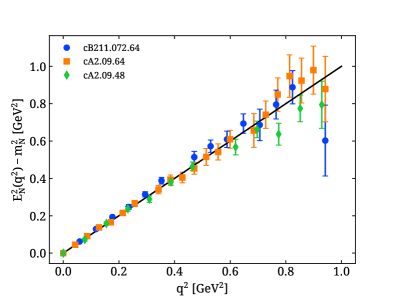
Figure 16: The difference between squared effective energy and squared effective mass obtained for the $\textrm{N}_{\textrm{f}}{=}2{+}1{+}1$ (blue circles), the large $\textrm{N}_{\textrm{f}}{=}2$ (orange squares), and the small $\textrm{N}_{\textrm{f}}{=}2$ (green diamonds) ensembles as a function of the spatial momentum squared. The black line is the continuum dispersion relation $E^{2}_{N}(q^{2})-m_{N}^{2}=q^{2}$.

Appendix C Tables of Results

Results for the GFFs are provided for $A_{20}(Q^{2})$, $B_{20}(Q^{2})$, $\tilde{A}_{20}(Q^{2})$, and $\tilde{B}_{20}(Q^{2})$ using the two-state fit method as explained in the text. We do not provide $C_{20}$ which is found to be consistent with zero. We provide results for ensemble cB211.072.64 in Table 8, for cA2.09.48 in Table 9, and for cA2.09.64 in Table 10.

Table 8: GFFs for ensemble cB211.072.64 obtained using the two-state fit method. We do not provide $C_{20}$ which is found to be consistent with zero.

$Q^{2}$ [GeV2]	$A_{20}(Q^{2})$	$B_{20}(Q^{2})$	$\tilde{A}_{20}(Q^{2})$	$\tilde{B}_{20}(Q^{2})$
0.000	0.178(16)		0.193(18)
0.058	0.165(19)	0.137(46)	0.182(16)	0.30(32)
0.114	0.140(15)	0.157(31)	0.163(16)	0.07(16)
0.169	0.128(16)	0.159(29)	0.149(17)	0.24(15)
0.222	0.150(21)	0.075(42)	0.152(15)	0.25(15)
0.273	0.125(14)	0.130(27)	0.143(14)	0.127(85)
0.324	0.119(15)	0.132(27)	0.130(15)	0.179(82)
0.421	0.117(16)	0.108(30)	0.127(14)	0.130(89)
0.468	0.119(14)	0.124(26)	0.119(14)	0.153(64)
0.514	0.115(15)	0.112(23)	0.118(14)	0.207(72)
0.559	0.121(15)	0.123(17)	0.107(14)	0.032(72)
0.603	0.107(22)	0.095(36)	0.110(16)	0.065(97)
0.647	0.115(16)	0.092(31)	0.102(15)	0.143(63)
0.690	0.143(15)	0.078(13)	0.094(15)	0.061(63)
0.773	0.087(21)	0.096(36)	0.116(17)	0.22(12)
0.814	0.116(18)	0.107(31)	0.086(15)	0.114(58)
0.854	0.114(20)	0.118(32)	0.093(15)	0.123(63)
0.893	0.131(21)	0.069(42)	0.112(15)	0.202(74)
0.932	0.115(22)	0.085(36)	0.079(16)	0.125(68)
0.970	0.138(17)	0.109(15)	0.080(16)	0.022(67)

Table 9: GFFs for ensemble cA2.09.48 obtained using the two-state fit method. We do not provide $C_{20}$ which is found to be consistent with zero.

$Q^{2}$ [GeV2]	$A_{20}(Q^{2})$	$B_{20}(Q^{2})$	$\tilde{A}_{20}(Q^{2})$	$\tilde{B}_{20}(Q^{2})$
0.000	0.167(13)		0.221(12)
0.075	0.176(24)	0.191(49)	0.197(18)	0.12(26)
0.146	0.144(20)	0.182(38)	0.192(16)	0.53(17)
0.215	0.120(24)	0.207(36)	0.167(19)	0.37(17)
0.282	0.103(31)	0.180(43)	0.158(16)	0.20(13)
0.346	0.124(20)	0.173(28)	0.144(17)	0.220(90)
0.409	0.109(22)	0.162(31)	0.142(16)	0.294(86)
0.529	0.102(26)	0.180(33)	0.115(18)	0.233(91)
0.586	0.088(27)	0.171(32)	0.115(17)	0.154(73)
0.643	0.108(23)	0.081(34)	0.097(18)	0.130(74)
0.698	0.114(24)	0.125(31)	0.104(15)	0.160(68)
0.751	0.105(38)	0.176(52)	0.089(23)	0.053(82)
0.804	0.092(33)	0.204(44)	0.095(18)	0.026(59)
0.855	0.072(41)	0.196(47)	0.092(22)	0.132(71)

Table 10: GFFs for ensemble cA2.09.64 obtained using the two-state fit method. We do not provide $C_{20}$ which is found to be consistent with zero.

$Q^{2}$ [GeV2]	$A_{20}(Q^{2})$	$B_{20}(Q^{2})$	$\tilde{A}_{20}(Q^{2})$	$\tilde{B}_{20}(Q^{2})$
0	0.189(23)		0.217(24)
0.042	0.197(18)	0.133(63)	0.218(20)	1.32(48)
0.083	0.187(18)	0.206(43)	0.206(19)	0.67(20)
0.123	0.176(19)	0.209(41)	0.198(19)	0.59(21)
0.163	0.141(34)	0.220(43)	0.185(19)	0.29(19)
0.201	0.174(17)	0.191(33)	0.177(19)	0.34(11)
0.239	0.173(17)	0.160(35)	0.169(19)	0.30(11)
0.312	0.167(17)	0.162(32)	0.158(18)	0.31(10)
0.348	0.157(18)	0.142(29)	0.151(18)	0.254(83)
0.383	0.159(18)	0.162(32)	0.148(16)	0.038(69)
0.417	0.160(16)	0.155(25)	0.141(17)	0.081(72)
0.451	0.144(21)	0.151(39)	0.138(19)	0.22(12)
0.484	0.159(17)	0.120(26)	0.131(18)	0.169(77)
0.517	0.145(19)	0.117(29)	0.130(17)	0.210(71)
0.581	0.130(38)	0.204(51)	0.149(14)	0.044(87)
0.612	0.136(19)	0.148(28)	0.127(14)	0.081(63)
0.643	0.143(19)	0.137(26)	0.126(15)	0.153(64)
0.674	0.131(21)	0.126(34)	0.124(16)	0.255(70)
0.704	0.135(21)	0.142(31)	0.120(15)	0.133(70)
0.734	0.144(19)	0.122(25)	0.119(15)	0.137(60)
0.763	0.093(30)	0.128(40)	0.113(16)	0.079(80)
0.821	0.138(22)	0.110(31)	0.103(16)	0.057(63)

Appendix D Comparison with previous results

The results presented here for the small $\textrm{N}_{\textrm{f}}{=}2$ ensemble, cA2.09.48, are an update to those first presented in Ref. Abdel-Rehim et al. (2015). For completeness, in Fig. 17 we compare the current results with those obtained in Ref. Abdel-Rehim et al. (2015).

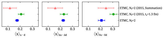
Figure 17: Results for the moments obtained on the cA2.09.48 ensemble as obtained in this work (blue squares) compared to previous results as presented in Ref. Abdel-Rehim et al. (2015) using the plateau method at the largest sink-source separation available at that time ($t_{s}=1.3$ fm, green circles) and the summation method (red triangles).

References

- Ji (2013) X. Ji, Phys. Rev. Lett. 110, 262002 (2013), eprint 1305.1539.
- Abdel-Rehim et al. (2017) A. Abdel-Rehim, C. Alexandrou, F. Burger, M. Constantinou, P. Dimopoulos, R. Frezzotti, K. Hadjiyiannakou, C. Helmes, K. Jansen, C. Jost, et al. (ETM), Phys. Rev. D95, 094515 (2017), eprint 1507.05068.
- Alexandrou et al. (2018a) C. Alexandrou et al., Phys. Rev. D98, 054518 (2018a), eprint 1807.00495.
- Aoki et al. (2019) S. Aoki et al. (Flavour Lattice Averaging Group) (2019), eprint 1902.08191.
- Osterwalder and Seiler (1978) K. Osterwalder and E. Seiler, Annals Phys. 110, 440 (1978).
- Alexandrou and Kallidonis (2017) C. Alexandrou and C. Kallidonis, Phys. Rev. D96, 034511 (2017), eprint 1704.02647.
- Alexandrou et al. (2018b) C. Alexandrou, S. Bacchio, M. Constantinou, J. Finkenrath, K. Hadjiyiannakou, K. Jansen, G. Koutsou, and A. V. A. Casco (2018b), eprint 1812.10311.
- Frezzotti et al. (2001) R. Frezzotti, P. A. Grassi, S. Sint, and P. Weisz (Alpha), JHEP 08, 058 (2001), eprint hep-lat/0101001.
- Frezzotti and Rossi (2004a) R. Frezzotti and G. C. Rossi, JHEP 08, 007 (2004a), eprint hep-lat/0306014.
- Sheikholeslami and Wohlert (1985) B. Sheikholeslami and R. Wohlert, Nucl. Phys. B259, 572 (1985).
- Frezzotti and Rossi (2004b) R. Frezzotti and G. C. Rossi, JHEP 10, 070 (2004b), eprint hep-lat/0407002.
- Frezzotti et al. (2006) R. Frezzotti, G. Martinelli, M. Papinutto, and G. C. Rossi, JHEP 04, 038 (2006), eprint hep-lat/0503034.
- Boucaud et al. (2008) P. Boucaud et al. (ETM), Comput. Phys. Commun. 179, 695 (2008), eprint 0803.0224.
- Chiarappa et al. (2007) T. Chiarappa, F. Farchioni, K. Jansen, I. Montvay, E. E. Scholz, L. Scorzato, T. Sudmann, and C. Urbach, Eur. Phys. J. C50, 373 (2007), eprint hep-lat/0606011.
- Abdel-Rehim et al. (2015) A. Abdel-Rehim et al., Phys. Rev. D92, 114513 (2015), [Erratum: Phys. Rev.D93,no.3,039904(2016)], eprint 1507.04936.
- Alexandrou et al. (1994) C. Alexandrou, S. Gusken, F. Jegerlehner, K. Schilling, and R. Sommer, Nucl. Phys. B414, 815 (1994), eprint hep-lat/9211042.
- Gusken (1990) S. Gusken, Nucl. Phys. Proc. Suppl. 17, 361 (1990).
- Albanese et al. (1987) M. Albanese et al. (APE), Phys. Lett. B192, 163 (1987).
- Alexandrou et al. (2013) C. Alexandrou, M. Constantinou, S. Dinter, V. Drach, K. Jansen, C. Kallidonis, and G. Koutsou, Phys. Rev. D88, 014509 (2013), eprint 1303.5979.
- Alexandrou et al. (2011a) C. Alexandrou, M. Brinet, J. Carbonell, M. Constantinou, P. A. Harraud, P. Guichon, K. Jansen, T. Korzec, and M. Papinutto, Phys. Rev. D83, 094502 (2011a), eprint 1102.2208.
- Alexandrou et al. (2006) C. Alexandrou, G. Koutsou, J. W. Negele, and A. Tsapalis, Phys. Rev. D74, 034508 (2006), eprint hep-lat/0605017.
- Maiani et al. (1987) L. Maiani, G. Martinelli, M. L. Paciello, and B. Taglienti, Nucl. Phys. B293, 420 (1987).
- Capitani et al. (2012) S. Capitani, M. Della Morte, G. von Hippel, B. Jager, A. Juttner, B. Knippschild, H. B. Meyer, and H. Wittig, Phys. Rev. D86, 074502 (2012), eprint 1205.0180.
- Bali et al. (2018) G. S. Bali, S. Collins, M. Göckeler, R. Rödl, A. Schäfer, and A. Sternbeck (2018), eprint 1812.08256.
- Bacchio et al. (2018) S. Bacchio, C. Alexandrou, and J. Finkerath, EPJ Web Conf. 175, 02002 (2018), eprint 1710.06198.
- Bacchio et al. (2016) S. Bacchio, C. Alexandrou, J. Finkenrath, A. Frommer, K. Kahl, and M. Rottmann, PoS LATTICE2016, 259 (2016), eprint 1611.01034.
- Alexandrou et al. (2016) C. Alexandrou, S. Bacchio, J. Finkenrath, A. Frommer, K. Kahl, and M. Rottmann, Phys. Rev. D94, 114509 (2016), eprint 1610.02370.
- Alexandrou et al. (2017) C. Alexandrou, M. Constantinou, and H. Panagopoulos, Phys. Rev. D95, 034505 (2017), eprint 1509.00213.
- Martinelli et al. (1995) G. Martinelli, C. Pittori, C. T. Sachrajda, M. Testa, and A. Vladikas, Nucl. Phys. B445, 81 (1995), eprint hep-lat/9411010.
- Gockeler et al. (1999) M. Gockeler, R. Horsley, H. Oelrich, H. Perlt, D. Petters, P. E. L. Rakow, A. Schafer, G. Schierholz, and A. Schiller, Nucl. Phys. B544, 699 (1999), eprint hep-lat/9807044.
- Alexandrou et al. (2011b) C. Alexandrou, M. Constantinou, T. Korzec, H. Panagopoulos, and F. Stylianou, Phys. Rev. D83, 014503 (2011b), eprint 1006.1920.
- Alexandrou et al. (2012) C. Alexandrou, M. Constantinou, T. Korzec, H. Panagopoulos, and F. Stylianou, Phys. Rev. D86, 014505 (2012), eprint 1201.5025.
- Constantinou et al. (2010) M. Constantinou et al. (ETM), JHEP 08, 068 (2010), eprint 1004.1115.
- Constantinou et al. (2015) M. Constantinou, R. Horsley, H. Panagopoulos, H. Perlt, P. E. L. Rakow, G. Schierholz, A. Schiller, and J. M. Zanotti, Phys. Rev. D91, 014502 (2015), eprint 1408.6047.
- Bar (2019) O. Bar, Phys. Rev. D99, 054506 (2019), eprint 1812.09191.
- von Hippel et al. (2017) G. von Hippel, T. D. Rae, E. Shintani, and H. Wittig, Nucl. Phys. B914, 138 (2017), eprint 1605.00564.
- Hill and Paz (2010) R. J. Hill and G. Paz, Phys. Rev. D82, 113005 (2010), eprint 1008.4619.
- Goeke et al. (2007) K. Goeke, J. Grabis, J. Ossmann, M. V. Polyakov, P. Schweitzer, A. Silva, and D. Urbano, Phys. Rev. D75, 094021 (2007), eprint hep-ph/0702030.
- Lorcé et al. (2019) C. Lorcé, H. Moutarde, and A. P. Trawiński, Eur. Phys. J. C79, 89 (2019), eprint 1810.09837.
- Bhattacharya et al. (2011) B. Bhattacharya, R. J. Hill, and G. Paz, Phys. Rev. D84, 073006 (2011), eprint 1108.0423.
- Lin et al. (2018) H.-W. Lin et al., Prog. Part. Nucl. Phys. 100, 107 (2018), eprint 1711.07916.
- Harris et al. (2019) T. Harris, G. von Hippel, P. Junnarkar, H. B. Meyer, K. Ottnad, J. Wilhelm, H. Wittig, and L. Wrang, Phys. Rev. D100, 034513 (2019), eprint 1905.01291.
- Green et al. (2014) J. R. Green, M. Engelhardt, S. Krieg, J. W. Negele, A. V. Pochinsky, and S. N. Syritsyn, Phys. Lett. B734, 290 (2014), eprint 1209.1687.
- Ball et al. (2017) R. D. Ball et al. (NNPDF), Eur. Phys. J. C77, 663 (2017), eprint 1706.00428.
- Dulat et al. (2016) S. Dulat, T.-J. Hou, J. Gao, M. Guzzi, J. Huston, P. Nadolsky, J. Pumplin, C. Schmidt, D. Stump, and C. P. Yuan, Phys. Rev. D93, 033006 (2016), eprint 1506.07443.
- Harland-Lang et al. (2015) L. A. Harland-Lang, A. D. Martin, P. Motylinski, and R. S. Thorne, Eur. Phys. J. C75, 204 (2015), eprint 1412.3989.
- Alekhin, S. and Blümlein, J. and Moch, S. and Placakyte, R. (2017) Alekhin, S. and Blümlein, J. and Moch, S. and Placakyte, R., Phys. Rev. D96, 014011 (2017), eprint 1701.05838.
- Accardi et al. (2016) A. Accardi, L. T. Brady, W. Melnitchouk, J. F. Owens, and N. Sato, Phys. Rev. D93, 114017 (2016), eprint 1602.03154.
- Abramowicz et al. (2015) H. Abramowicz et al. (H1, ZEUS), Eur. Phys. J. C75, 580 (2015), eprint 1506.06042.
- Blümlein, Johannes and Böttcher, Helmut (2010) Blümlein, Johannes and Böttcher, Helmut, Nucl. Phys. B841, 205 (2010), eprint 1005.3113.
- Nocera et al. (2014) E. R. Nocera, R. D. Ball, S. Forte, G. Ridolfi, and J. Rojo (NNPDF), Nucl. Phys. B887, 276 (2014), eprint 1406.5539.
- de Florian et al. (2009) D. de Florian, R. Sassot, M. Stratmann, and W. Vogelsang, Phys. Rev. D80, 034030 (2009), eprint 0904.3821.
- Ethier et al. (2017) J. J. Ethier, N. Sato, and W. Melnitchouk, Phys. Rev. Lett. 119, 132001 (2017), eprint 1705.05889.
- Lorcé (2014) C. Lorcé, Phys. Lett. B735, 344 (2014), eprint 1401.7784.
- Bhoonah and Lorcé (2017) A. Bhoonah and C. Lorcé, Phys. Lett. B774, 435 (2017), eprint 1703.08322.
- Ji (1997) X.-D. Ji, Phys. Rev. Lett. 78, 610 (1997), eprint hep-ph/9603249.
- Jülich Supercomputing Centre (2015) Jülich Supercomputing Centre, Journal of large-scale research facilities 1 (2015), URL http://dx.doi.org/10.17815/jlsrf-1-18.
- Jülich Supercomputing Centre (2018) Jülich Supercomputing Centre, Journal of large-scale research facilities 4 (2018), URL http://dx.doi.org/10.17815/jlsrf-4-121-1.
- Jülich Supercomputing Centre (2019) Jülich Supercomputing Centre, Journal of large-scale research facilities 5 (2019), URL http://dx.doi.org/10.17815/jlsrf-5-171.