Primordial non-Gaussianities of scalar and tensor perturbations in general bounce cosmology: Evading the no-go theorem
Abstract
It has been pointed out that matter bounce cosmology driven by a k-essence field cannot satisfy simultaneously the observational bounds on the tensor-to-scalar ratio and non-Gaussianity of the curvature perturbation. In this paper, we show that this is not the case in more general scalar-tensor theories. To do so, we evaluate the power spectra and the bispectra of scalar and tensor perturbations on a general contracting background in the Horndeski theory. We then discuss how one can discriminate contracting models from inflation based on non-Gaussian signatures of tensor perturbations.
pacs:
98.80.Cq, 04.50.KdI Introduction
Although it is definite that inflation Guth:1980zm ; Starobinsky:1980te ; Sato:1980yn is the most successful early universe model, it is inevitably plagued by the initial singularity problem Borde:1996pt . Motivated by this, alternative scenarios which do not suffer from this problem have also been explored (see, e.g., Battefeld:2014uga for a review). Non-singular cosmology has its own difficulty regarding gradient instabilities when constructed within second-order scalar-tensor theories Libanov:2016kfc ; Kobayashi:2016xpl ; Cai:2016thi ; Creminelli:2016zwa ; Akama:2017jsa , but its resolution has been proposed in the context of higher-order scalar-tensor theories Cai:2016thi ; Creminelli:2016zwa ; Cai:2017tku ; Cai:2017dyi ; Kolevatov:2017voe ; Ye:2019frg ; Ye:2019sth . It is also important to discuss the validity of non-singular alternatives from the viewpoint of cosmological observations.
For example, a matter-dominated contracting (or bounce) universe can be mimicked by a canonical scalar field and this model can generate a scale-invariant curvature perturbations Wands:1998yp ; Finelli:2001sr ; Quintin:2015rta . However, this model yields a too large tensor-to-scalar ratio and thus is excluded Quintin:2015rta (see, however, Refs. Raveendran:2017vfx ; Raveendran:2018why ). One may use a k-essence field to reduce the tensor-to-scalar ratio by taking a small sound speed, but then this in turn enhances the production of non-Gaussianity, making the model inconsistent with observations Li:2016xjb . At this stage, it is not evident whether or not this “no-go theorem” holds in more general scalar-tensor theories.
The purpose of the present paper is clarifying to what extent the previous no-go theorem (which was formulated in the context of a k-essence field minimally coupled to gravity as an extension of Ref. Quintin:2015rta ) holds in more general setups. To do so, we consider a general power-law contracting universe in the Horndeski theory Horndeski:1974wa , the most general second-order scalar-tensor theory, and evaluate the power spectra and the bispectra of scalar and tensor perturbations generated during the contracting phase. Throughout the paper we assume that the statistical nature of these primordial perturbations does not change during the subsequent bouncing and expanding phases. (In some cases in matter bounce cosmology, this has been justified. See, e.g., Ref. Gao:2009wn .) In calculating tensor non-Gaussianity we explore peculiar signatures of a contracting phase as compared to inflation, and show that the two scenarios can potentially be distinguishable due to the non-Gaussian amplitudes and shapes.
This paper is organized as follows. In the next section, we introduce our setup of the general contracting cosmological background. In Sec. III, we evaluate the power spectra for curvature and tensor perturbations, and derive the conditions under which they are scale-invariant. In Sec. IV, we calculate primordial non-Gaussianities of curvature and tensor perturbations, and investigate whether a small tensor-to scalar ratio and small scalar non-Gaussianity are compatible or not in the Horndeski theory. We also discuss how one can distinguish bounce cosmology with inflation based on tensor non-Gaussianity. The conclusion of this paper is drawn in Sec. V.
II Setup
We begin with a spatially flat Friedmann-Lemaître-Robertson-Walker (FLRW) metric
| (1) |
where the scale factor describes a contracting phase,
| (2) |
with . Here, we denoted the time at the end of the contracting phase as and , and we normalized the scale factor so that . The two time coordinates are related with
| (3) |
where and coordinates run from to and , respectively. In this paper, we do not assume to take any particular value, so that our setup includes models other than the familiar matter bounce scenario Brandenberger:2012zb . Note, however, that it will turn out that models with different are related to each other via conformal transformation (see Sec. III.3).
We work with the Horndeski action which is given by
| (4) |
with
| (5) |
where and is denoted by . This action gives the most general second-order scalar-tensor theory, and hence a vast class of contracting scenarios reside within this theory. Therefore, the Horndeski theory is adequate for studying generic properties of cosmological perturbations from contracting models. Note, however, that nonsingular cosmological solutions suffer from gradient instabilities if the entire history of the universe were described by the Horndeski theory Libanov:2016kfc ; Kobayashi:2016xpl ; Cai:2016thi ; Creminelli:2016zwa ; Akama:2017jsa . We circumvent this issue by assuming that beyond-Horndeski operators come into play at some moment, but at least the contracting phase we are focusing on is assumed to be described by the Horndeski theory.
The Friedmann and evolution equations are written, respectively, in the form
| (6) |
where and come from the variation of the action involving , whose explicit expressions are given in Appendix A. Here a dot stands for differentiation with respect to and . In this paper, we do not consider any concrete background models, but just assume that each term in the background equations scales as
| (7) |
where is a constant to be specified below. The impact of spatial curvature and anisotropies is discussed in Appendix B.
III Scale-invariant power spectra
The perturbed metric in the unitary gauge, , is written as
| (8) |
where
| (9) | |||
| (10) |
As has been done in Ref. Kobayashi:2011nu , one expands the action to second order in perturbations and removes the auxiliary variables and . The resultant quadratic actions for the curvature perturbation and the tensor perturbations in the Horndeski theory are written, respectively, as
| (11) | ||||
| (12) |
where
| (13) | ||||
| (14) | ||||
| (15) | ||||
| (16) |
with
| (17) | ||||
| (18) |
(The explicit expressions for and are given in Appendix C.) As inferred from Eqs. (7), (17), and (18), it is natural to assume that and . In addition, it can be seen that . These imply
| (19) |
Under these assumptions, the propagation speed of the curvature perturbation, , and that of the tensor perturbations, , are constant. Note that only is possible if is minimally coupled to gravity.
Let us move to derive a relation between and by imposing that the primordial curvature and tensor perturbations have scale-invariant power spectra.
III.1 Curvature Perturbation
We expand and quantize the curvature perturbation as
| (20) | ||||
| (21) |
where the commutation relations between the creation and annihilation operators are standard ones,
| (22) | ||||
| (23) |
The mode function of the canonically normalized perturbation, , obeys
| (24) |
where a prime denotes differentiation with respect to and
| (25) |
The positive frequency solution is then given by
| (26) |
where is the Hankel function of the first kind. Here we chose the initial condition as
| (27) |
The power spectrum of the curvature perturbation is defined by
| (28) |
and therefore
| (29) |
The spectral index is thus given by
| (30) |
Let us focus on the exactly scale-invariant spectrum, which corresponds to
| (31) | ||||
| (32) |
On superhorizon scales, , we have . Therefore, the perturbations freeze out on superhorizon scales in the former case (as in the inflationary universe), while they grow as in the latter case (as in the contracting universe). In this paper, we consider the growing superhorizon perturbations having a scale-invariant spectrum, which is a characteristic feature of contracting models. Note that the Planck results Akrami:2018odb require a slightly red tilted spectrum, . This can be obtained by slightly detuning the relation (32) between and , though for simplicity in this paper we only consider the exactly scale-invariant case.
Taking , the scale-invariant power spectrum can now be derived as
| (33) |
where the time-dependent quantities are evaluated at the end of the contracting phase.
III.2 Tensor Perturbations
The tensor perturbations can be expanded and quantized as
| (34) | ||||
| (35) |
where the creation and annihilation operators satisfy the canonical commutation relations
| (36) | ||||
| (37) |
The two helicity modes are labeled by , and the basis satisfies the transverse and traceless conditions, , and it is normalized as .
The mode function of the canonically normalized perturbations, , obeys
| (38) |
where . The positive frequency solution is then given by
| (39) |
where one can see that
| (40) |
The behavior of the tensor perturbations is essentially the same as that of . For (), grows on superhorizon scales as and the tensor power spectrum is scale invariant.
Let us define by
| (41) |
Then,
| (42) |
with
| (43) |
and the tensor power spectrum is defined as . For , we have the scale-invariant power spectrum
| (44) |
where time-dependent quantities are evaluated at .
For example, in the case of matter contracting models within the k-essence theory, we have , , , and const. Therefore, the tensor-to-scalar ratio is
| (47) |
which can satisfy the upper bound on only for . However, as argued in Ref. Li:2016xjb , small implies large scalar non-Gaussianity, and hence bounce models within the k-essence theory are ruled out. In the next section, we revisit this issue and study whether or not upper bounds on the tensor-to-scalar ratio and non-Gaussianity can be satisfied at the same time in a wider class of theories.
III.3 Conformal Frames
At this stage it is instructive to perform a conformal transformation and clarify the relation among models with different .
Let us consider a conformally related metric
| (48) |
In this tilde frame, the time coordinate and the scale factor are given respectively by
| (49) | ||||
| (50) |
By inspecting the quadratic action for scalar and tensor perturbations we see that in the tilde frame all the four coefficients reduce to constants.
We find that the case of () can be regarded as de Sitter inflation (see, e.g., Ref. Nandi:2019xag ).
In the case of (), we have
| (51) |
which describes a matter-dominated contracting universe. Therefore, the dynamics of cosmological perturbations in our contracting models (with general ) is equivalent to that in the more familiar matter-dominated contracting model. However, it should be emphasized that the magnitudes of the coefficients in the perturbation action are still arbitrary even in the tilde frame.
IV Primordial non-Gaussianities
IV.1 Scalar Perturbations
The three-point correlation function can be computed by using the in-in formalism as
| (52) |
where
| (53) |
with being the cubic Lagrangian of the curvature perturbation. It can be written in the form Gao:2011qe ; DeFelice:2011uc ; Gao:2012ib
| (54) |
where and are dimensionless coefficients. The complete form of the cubic Lagrangian is summarized in Appendix C. Based on the scaling argument similar to that in the previous section, it can be seen that the coefficients are constant.
The last term in Eq. (54) can be eliminated by means of a field redefinition
| (55) |
In Fourier space, this redefinition is equivalent to
| (56) |
where
| (57) | ||||
| (58) |
Here we approximated the time derivative of the curvature perturbation on superhorizon scales as
| (59) |
and ignored sub-leading contributions denoted by the ellipsis ().
The bispectrum is defined by
| (60) |
where we write
| (61) |
and evaluate the amplitude . In our setup, reads
| (62) |
where and are the contributions respectively from the interaction Hamiltonian and from the field redefinition (56):
| (63) | ||||
| (64) |
One can check that the result of the calculation of the primordial bispectra involving the procedure of the field redefinition is identical to that involving boundary terms in the cubic action with the linear equation of motion being imposed. (See Refs. Arroja:2011yj ; Rigopoulos:2011eq ; Burrage:2011hd .) The explicit form of the boundary terms is given in Appendix C.
Based on the above result we also evaluate the nonlinearity parameter defined as
| (65) |
at the squeezed limit , the equilateral limit , and the folded limit . At these limits, the parameter is given respectively by
| (66) | ||||
| (67) | ||||
| (68) |
(Here we denoted the nonlinearity parameter at the squeezed limit as .)
In the case of the matter contracting models within the k-essence theory, these are written as
| (69) | ||||
| (70) | ||||
| (71) |
where . These results reproduce those in Li:2016xjb ; Cai:2009fn . In order for these nonlinearity parameters to be , one requires . In the context of k-essence, this leads to , which is ruled out. Instead one may take to have , but then the nonlinearity parameters are too large to be consistent with observations:
| (72) |
indicating that any matter bounce models in the k-essence theory are excluded. (Observational constraints are given by and Akrami:2019izv .)
Although small is incompatible with small scalar non-Gaussianity in the k-essence theory, this is not always the case in the Horndeski theory. Thanks to a sufficient number of independent functions, one can make small while retaining , , and less than . We will discuss this point in more detail in the next subsection.
IV.2 Example
Let us consider a concrete Lagrangian characterized by
| (73) |
where . We seek for a solution of the matter-dominated contracting universe, , with a time-dependent scalar field,
| (74) |
It then follows that const. This indeed solves the background equations provided that the functions and satisfy
| (75) | ||||
| (76) |
where a prime in this subsection denotes differentiation with respect to .
Let us further impose that
| (77) | ||||
| (78) |
where and are some small positive numbers, . We then have
| (79) |
and a small tensor-to-scalar ratio can be obtained, , while , which cannot be achieved in the k-essence theory.
A would-be dangerous contribution to comes from :
| (80) |
This can be made safe if one requires
| (81) |
where is another small number. All the other terms give at most contributions.
To sum up, by introducing the functions and satisfying the conditions (75), (76), (77), (78), and (81), one has and simultaneously. Clearly, this is indeed possible. One can thus circumvent the no-go theorem presented in Li:2016xjb by appropriately choosing the functions in the Lagrangian which is more general than the k-essence theory.
IV.3 Tensor Perturbations
The three-point correlation function including interactions among different polarization modes of tensor perturbations can be computed from
| (82) |
where . The interaction Hamiltonian, , is given by
| (83) |
where Gao:2011vs
| (84) |
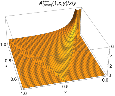
with which scales as , as seen from Eq. (19). The first term, , is the new contribution due to , while the second one, which is of the form , is identical to the corresponding term in general relativity except for the overall normalization. We attach the label “new” (respectively, “GR”) to the quantities associated with the former (respectively, latter) interaction.
Similarly to the case of the curvature perturbation, the bispectrum is defined by
| (85) |
where
| (86) | ||||
| (87) |
and we evaluate the amplitudes and . In our setup we obtain
| (88) | ||||
| (89) |
with
| (90) |
Figures 1 and 2 show that both and have peaks at the squeezed limit. Note that has a specific scale-dependence . This has been obtained in the context of matter bounce cosmology driven by a scalar field minimally coupled to gravity Chowdhury:2015cma . However, this factor makes the detection more challenging Kothari:2019yyw .

Now let us compare the above results with the prediction from generalized G-inflation Kobayashi:2011nu . The amplitudes of non-Gaussianities of tensor perturbations in (quasi-de Sitter) inflation are given by Gao:2011vs
| (91) | ||||
| (92) |
where
| (93) |
Let us first look at their shapes. As shown in Gao:2011vs , of inflation models has a peak at the equilateral limit. This is in contrast with the case of contracting models. On the other hand, has a peak at the squeezed limit both in inflation and contracting models. Therefore, the detection of the equilateral-type tensor non-Gaussianities would rule out our contracting models.
Next, let us compare the amplitudes. Squeezed tensor non-Gaussianity from inflation has the fixed amplitude, as Eq. (92) is independent of the functions in the Horndeski action. This is not the case for squeezed non-Gaussianity from contracting models, as is clear from Eqs. (88) and (89), whichever is dominant.
Finally, notice that the non-Gaussian amplitudes (88) and (89) agree with those obtained in a kind of non-attractor inflation models, where tensor perturbations grow on superhorizon scales during inflation due to non-attractor dynamics of the non-minimally coupled inflaton Ozsoy:2019slf . This is because both our contracting models and the non-attractor phase of inflation are conformally equivalent to the matter-dominated contracting scenario.
V Summary
In this paper, we have studied the primordial power spectra and the bispectra of scalar and tensor perturbations generated during a general contracting phase in the Horndeski theory. It can be shown that under certain conditions the power spectra of scalar and tensor perturbations are scale invariant. We have found that the previous no-go theorem Li:2016xjb prohibiting the simultaneous realization of small tensor-to-scalar ratio and small scalar non-Gaussianity in matter bounce cosmology driven by a k-essence field no longer holds in more general setups. A concrete example with small and small has been presented.
Then, we have found that the non-Gaussianities of tensor perturbations from the contracting universes have two specific features which are in contrast with the predictions from generalized G-inflation. First, our contracting models predict only squeezed-type non-Gaussianities, while inflation can in principle generate both squeezed- and equilateral-type ones. Second, the squeezed-type non-Gaussian amplitude from inflation is model-independently fixed, while that from the contracting scenario is model-dependent. We thus conclude that our general bounce model can be distinguished from generalized G-inflation by combining the information of the non-Gaussian amplitudes and shapes. It would be interesting to investigate the possibility to detect the non-Gaussian signatures predicted from the general bounce model through the B-mode polarization, as argued in Refs. Kothari:2019yyw ; Tahara:2017wud .
Acknowledgements.
We would like to thank Jerome Quintin for helpful correspondence. We thank Shuichiro Yokoyama for fruitful discussions. SH thanks Sakine Nishi and Kazufumi Takahashi for instructing him how to use Mathematica for the calculation of perturbations. The work of SA was supported by the JSPS Research Fellowships for Young Scientists No. 18J22305. The work of SH was supported by the JSPS Research Fellowships for Young Scientists No. 17J04865. The work of TK was supported by MEXT KAKENHI Grant Nos. JP15H05888, JP17H06359, JP16K17707, and JP18H04355.Appendix A Background Equations
For a flat FLRW universe the gravitational field equations read Kobayashi:2011nu
| (94) |
where
| (95) | ||||
| (96) | ||||
| (97) | ||||
| (98) |
and
| (99) | ||||
| (100) | ||||
| (101) | ||||
| (102) |
The scalar-field equation follows from the above two equations.
Appendix B Effects of Spatial Curvature and Anisotropies on a General Contracting Background
In the simple, standard case of a scalar field minimally coupled to gravity, spatial curvature and anisotropies in the Friedmann and evolution equations evolve in proportion to and , respectively. As a result, it has been known that a contracting universe is plagued with the instability associated with large anisotropies Belinsky:1970ew . Some resolutions of the problem have been proposed so far. See, e.g., Refs. Khoury:2001wf ; Lehners:2008vx ; Cai:2013vm ; Qiu:2013eoa ; Lin:2017fec . However, the impact of spatial curvature and anisotropies has not been clear yet in more general cases where the scalar field is nonminimally coupled to gravity. Hence, we investigate the evolution of spatial curvature and anisotropies in a general contracting background in the Horndeski theory.
First, we investigate the impact of spatial curvature (denoted hereafter as ). To do so, we consider open and closed universes in the Horndeski theory. In the presence of spatial curvature, the background equations reduce to Nishi:2015pta ; Akama:2018cqv
| (103) |
where
| (104) |
It can be seen from the scaling argument that , which implies that the relative magnitudes of the curvature terms decrease with time so that the effect of the spatial curvature on the background equations can be neglected in our setups.
Next, let us consider the effect of anisotropies on the contracting background by investigating an anisotropic Kasner universe whose metric is written as
| (105) |
The differences between the expansion rates in different directions, , obey Nishi:2015pta ; Tahara:2018orv
| (106) | ||||
| (107) |
Since we have , the nonlinear terms can be ignored as long as initially small anisotropies are considered, . Then, these equations can be integrated to give . We thus see that , which decreases with time if and increases if . The case of corresponds to the former, while to the latter. This result implies the contracting background we are considering requires some mechanism to evade the unwanted growth of anisotropies. In the present paper, we simply assume that the contracting universe enjoys a bounce before the anisotropies spoil its background evolution.
Appendix C Cubic Action for Scalar Perturbations in the Horndeski Theory
Substituting the perturbed metric (9) into the Horndeski action, expanding it to cubic order in perturbations and using the background equations, we obtain the cubic action for scalar perturbations Gao:2011qe ; DeFelice:2011uc ; Gao:2012ib :
| (108) |
From the first-order constraint equations we have
| (109) | ||||
| (110) |
where . Substituting these solutions into the cubic action, we obtain
| (111) |
where
| (112) | ||||
| (113) | ||||
| (114) | ||||
| (115) | ||||
| (116) | ||||
| (117) | ||||
| (118) | ||||
| (119) | ||||
| (120) | ||||
| (121) |
Here we defined
| (122) | ||||
| (123) | ||||
| (124) | ||||
| (125) |
and
| (126) |
Note that we can write the Eqs. (124), (125) as
| (127) |
It is therefore natural to assume that these quantities scale as
| (128) |
In Eq. (111), we neglected some boundary terms having the form of a total time derivative. They are given by
| (129) |
where
| (130) | ||||
| (131) |
References
- (1) A. H. Guth, “The Inflationary Universe: A Possible Solution to the Horizon and Flatness Problems,” Phys. Rev. D 23, 347 (1981).
- (2) A. A. Starobinsky, “A New Type of Isotropic Cosmological Models Without Singularity,” Phys. Lett. B 91, 99 (1980).
- (3) K. Sato, “First Order Phase Transition of a Vacuum and Expansion of the Universe,” Mon. Not. Roy. Astron. Soc. 195, 467 (1981).
- (4) A. Borde and A. Vilenkin, “Singularities in inflationary cosmology: A Review,” Int. J. Mod. Phys. D 5, 813 (1996) [gr-qc/9612036].
- (5) D. Battefeld and P. Peter, “A Critical Review of Classical Bouncing Cosmologies,” Phys. Rept. 571, 1 (2015) [arXiv:1406.2790 [astro-ph.CO]].
- (6) M. Libanov, S. Mironov and V. Rubakov, “Generalized Galileons: instabilities of bouncing and Genesis cosmologies and modified Genesis,” JCAP 1608, no. 08, 037 (2016) [arXiv:1605.05992 [hep-th]].
- (7) T. Kobayashi, “Generic instabilities of nonsingular cosmologies in Horndeski theory: A no-go theorem,” Phys. Rev. D 94, no. 4, 043511 (2016) [arXiv:1606.05831 [hep-th]].
- (8) Y. Cai, Y. Wan, H. G. Li, T. Qiu and Y. S. Piao, “The Effective Field Theory of nonsingular cosmology,” JHEP 1701, 090 (2017) [arXiv:1610.03400 [gr-qc]].
- (9) P. Creminelli, D. Pirtskhalava, L. Santoni and E. Trincherini, “Stability of Geodesically Complete Cosmologies,” JCAP 1611, no. 11, 047 (2016) [arXiv:1610.04207 [hep-th]].
- (10) S. Akama and T. Kobayashi, “Generalized multi-Galileons, covariantized new terms, and the no-go theorem for nonsingular cosmologies,” Phys. Rev. D 95, no. 6, 064011 (2017) [arXiv:1701.02926 [hep-th]].
- (11) Y. Cai, H. G. Li, T. Qiu and Y. S. Piao, “The Effective Field Theory of nonsingular cosmology: II,” Eur. Phys. J. C 77, no. 6, 369 (2017) [arXiv:1701.04330 [gr-qc]].
- (12) Y. Cai and Y. S. Piao, “A covariant Lagrangian for stable nonsingular bounce,” JHEP 1709, 027 (2017) [arXiv:1705.03401 [gr-qc]].
- (13) R. Kolevatov, S. Mironov, N. Sukhov and V. Volkova, “Cosmological bounce and Genesis beyond Horndeski,” JCAP 1708, no. 08, 038 (2017) [arXiv:1705.06626 [hep-th]].
- (14) G. Ye and Y. S. Piao, “Implication of GW170817 for cosmological bounces,” Commun. Theor. Phys. 71, no. 4, 427 (2019) [arXiv:1901.02202 [gr-qc]].
- (15) G. Ye and Y. S. Piao, “Bounce in general relativity and higher-order derivative operators,” Phys. Rev. D 99, no. 8, 084019 (2019) [arXiv:1901.08283 [gr-qc]].
- (16) D. Wands, “Duality invariance of cosmological perturbation spectra,” Phys. Rev. D 60, 023507 (1999) [gr-qc/9809062].
- (17) F. Finelli and R. Brandenberger, “On the generation of a scale invariant spectrum of adiabatic fluctuations in cosmological models with a contracting phase,” Phys. Rev. D 65, 103522 (2002) [hep-th/0112249].
- (18) J. Quintin, Z. Sherkatghanad, Y. F. Cai and R. H. Brandenberger, “Evolution of cosmological perturbations and the production of non-Gaussianities through a nonsingular bounce: Indications for a no-go theorem in single field matter bounce cosmologies,” Phys. Rev. D 92, no. 6, 063532 (2015) [arXiv:1508.04141 [hep-th]].
- (19) R. N. Raveendran, D. Chowdhury and L. Sriramkumar, “Viable tensor-to-scalar ratio in a symmetric matter bounce,” JCAP 1801, 030 (2018) [arXiv:1703.10061 [gr-qc]].
- (20) R. N. Raveendran and L. Sriramkumar, “Viable scalar spectral tilt and tensor-to-scalar ratio in near-matter bounces,” arXiv:1812.06803 [astro-ph.CO].
- (21) Y. B. Li, J. Quintin, D. G. Wang and Y. F. Cai, “Matter bounce cosmology with a generalized single field: non-Gaussianity and an extended no-go theorem,” JCAP 1703, no. 03, 031 (2017) [arXiv:1612.02036 [hep-th]].
- (22) G. W. Horndeski, “Second-order scalar-tensor field equations in a four-dimensional space,” Int. J. Theor. Phys. 10, 363 (1974).
- (23) X. Gao, Y. Wang, W. Xue and R. Brandenberger, “Fluctuations in a Horava-Lifshitz Bouncing Cosmology,” JCAP 1002, 020 (2010) [arXiv:0911.3196 [hep-th]].
- (24) R. H. Brandenberger, “The Matter Bounce Alternative to Inflationary Cosmology,” arXiv:1206.4196 [astro-ph.CO].
- (25) T. Kobayashi, M. Yamaguchi and J. Yokoyama, “Generalized G-inflation: Inflation with the most general second-order field equations,” Prog. Theor. Phys. 126, 511 (2011) [arXiv:1105.5723 [hep-th]].
- (26) Y. Akrami et al. [Planck Collaboration], “Planck 2018 results. X. Constraints on inflation,” arXiv:1807.06211 [astro-ph.CO].
- (27) D. Nandi and L. Sriramkumar, “Can non-minimal coupling restore the consistency condition in bouncing universes?,” arXiv:1904.13254 [gr-qc].
- (28) X. Gao and D. A. Steer, “Inflation and primordial non-Gaussianities of ’generalized Galileons’,” JCAP 1112, 019 (2011) [arXiv:1107.2642 [astro-ph.CO]].
- (29) A. De Felice and S. Tsujikawa, “Inflationary non-Gaussianities in the most general second-order scalar-tensor theories,” Phys. Rev. D 84, 083504 (2011) [arXiv:1107.3917 [gr-qc]].
- (30) X. Gao, T. Kobayashi, M. Shiraishi, M. Yamaguchi, J. Yokoyama and S. Yokoyama, “Full bispectra from primordial scalar and tensor perturbations in the most general single-field inflation model,” PTEP 2013, 053E03 (2013) [arXiv:1207.0588 [astro-ph.CO]].
- (31) F. Arroja and T. Tanaka, “A note on the role of the boundary terms for the non-Gaussianity in general k-inflation,” JCAP 1105, 005 (2011) [arXiv:1103.1102 [astro-ph.CO]].
- (32) G. Rigopoulos, “Gauge invariance and non-Gaussianity in Inflation,” Phys. Rev. D 84, 021301 (2011) [arXiv:1104.0292 [astro-ph.CO]].
- (33) C. Burrage, R. H. Ribeiro and D. Seery, “Large slow-roll corrections to the bispectrum of noncanonical inflation,” JCAP 1107, 032 (2011) [arXiv:1103.4126 [astro-ph.CO]].
- (34) Y. F. Cai, W. Xue, R. Brandenberger and X. Zhang, “Non-Gaussianity in a Matter Bounce,” JCAP 0905, 011 (2009) [arXiv:0903.0631 [astro-ph.CO]].
- (35) Y. Akrami et al. [Planck Collaboration], “Planck 2018 results. IX. Constraints on primordial non-Gaussianity,” arXiv:1905.05697 [astro-ph.CO].
- (36) X. Gao, T. Kobayashi, M. Yamaguchi and J. Yokoyama, “Primordial non-Gaussianities of gravitational waves in the most general single-field inflation model,” Phys. Rev. Lett. 107, 211301 (2011) [arXiv:1108.3513 [astro-ph.CO]].
- (37) D. Chowdhury, V. Sreenath and L. Sriramkumar, “The tensor bi-spectrum in a matter bounce,” JCAP 1511, 002 (2015) [arXiv:1506.06475 [astro-ph.CO]].
- (38) R. Kothari and D. Nandi, “B-Mode auto-bispectrum due to matter bounce,” arXiv:1901.06538 [astro-ph.CO].
- (39) O. Ozsoy, M. Mylova, S. Parameswaran, C. Powell, G. Tasinato and I. Zavala, “Squeezed tensor non-Gaussianity in non-attractor inflation,” arXiv:1902.04976 [hep-th].
- (40) H. W. H. Tahara and J. Yokoyama, “CMB B-mode auto-bispectrum produced by primordial gravitational waves,” PTEP 2018, no. 1, 013E03 (2018) [arXiv:1704.08904 [astro-ph.CO]].
- (41) V. A. Belinsky, I. M. Khalatnikov and E. M. Lifshitz, “Oscillatory approach to a singular point in the relativistic cosmology,” Adv. Phys. 19, 525 (1970).
- (42) J. Khoury, B. A. Ovrut, P. J. Steinhardt and N. Turok, “The Ekpyrotic universe: Colliding branes and the origin of the hot big bang,” Phys. Rev. D 64, 123522 (2001) [hep-th/0103239].
- (43) J. L. Lehners, “Ekpyrotic and Cyclic Cosmology,” Phys. Rept. 465, 223 (2008) [arXiv:0806.1245 [astro-ph]].
- (44) Y. F. Cai, R. Brandenberger and P. Peter, “Anisotropy in a Nonsingular Bounce,” Class. Quant. Grav. 30, 075019 (2013) [arXiv:1301.4703 [gr-qc]].
- (45) T. Qiu, X. Gao and E. N. Saridakis, “Towards anisotropy-free and nonsingular bounce cosmology with scale-invariant perturbations,” Phys. Rev. D 88, no. 4, 043525 (2013) [arXiv:1303.2372 [astro-ph.CO]].
- (46) C. Lin, J. Quintin and R. H. Brandenberger, “Massive gravity and the suppression of anisotropies and gravitational waves in a matter-dominated contracting universe,” JCAP 1801, 011 (2018) [arXiv:1711.10472 [hep-th]].
- (47) S. Nishi and T. Kobayashi, “Generalized Galilean Genesis,” JCAP 1503, no. 03, 057 (2015) [arXiv:1501.02553 [hep-th]].
- (48) S. Akama and T. Kobayashi, “General theory of cosmological perturbations in open and closed universes from the Horndeski action,” Phys. Rev. D 99, no. 4, 043522 (2019) [arXiv:1810.01863 [gr-qc]].
- (49) H. W. H. Tahara, S. Nishi, T. Kobayashi and J. Yokoyama, “Self-anisotropizing inflationary universe in Horndeski theory and beyond,” JCAP 1807, no. 07, 058 (2018) [arXiv:1805.00186 [gr-qc]].