Method and System for Image Analysis to Detect Cancer

Abstract

Breast cancer is the most common cancer and is the leading cause of cancer death among women worldwide. Detection of breast cancer, while it is still small and confined to the breast, provides the best chance of effective treatment. Computer Aided Detection (CAD) systems that detect cancer from mammograms will help in reducing the human errors that lead to missing breast carcinoma. Literature is rich of scientific papers for methods of CAD design, yet with no complete system architecture to deploy those methods. On the other hand, commercial CADs are developed and deployed only to vendors’ mammography machines with no availability to public access. This paper presents a complete CAD; it is complete since it combines, on a hand, the rigor of algorithm design and assessment (method), and, on the other hand, the implementation and deployment of a system architecture for public accessibility (system). (1) We develop a novel algorithm for image enhancement so that mammograms acquired from any digital mammography machine look qualitatively of the same clarity to radiologists’ inspection; and is quantitatively standardized for the detection algorithms. (2) We develop novel algorithms for masses and microcalcifications detection with accuracy superior to both literature results and the majority of approved commercial systems. (3) We design, implement, and deploy a system architecture that is computationally effective to allow for deploying these algorithms to cloud for public access.

left=0.65in, right=0.65in, top=0.70in, bottom=0.70in

1 Introduction

1.1 Breast Cancer and Computer Aided Detection (CAD)

Breast cancer is the most common cancer in women in developed Western countries and is becoming ever more significant in many developing countries [2]. Although incidence rates are increasing, mortality rates are stable, representing an improved survival rate. This improvement can be attributed to effective means of early detection, mainly mammography, as well as to significant improvement in treatment options [3]. Moreover, “Breast carcinoma is not a systemic disease at its inception, but is a progressive disease and its development can be arrested by screening” [4, 5]. Early detection of breast cancer, while it is still small and confined to the breast, provides the best chance of effective treatment for women with the disease [6, 7].

Detection of breast cancer on mammography is performed by a human reader, usually radiologist or oncologist. Causes of missed breast cancer on mammography can be secondary to many factors including those related to the patient (whether inherent or acquired), the nature of the malignant mass itself, poor mammography techniques, or interpretive skills of the human reader (including perception and interpretation errors) [8]. Perception error occurs when the lesion is included in the field of view and is evident but is not recognized by the radiologist. The lesion may or may not have subtle features of malignancy that cause it to be less visible. Small nonspiculated masses, areas of architectural distortion, asymmetry, small clusters of amorphous, or faint microcalcifications, all may be difficult to perceive [8]. On the other hand, interpretation error occurs for several reasons including lack of experience, fatigue, or inattention. It may also occur if the radiologist fails to obtain all the views needed to assess the characteristics of a lesion or if the lesion is slow growing and prior images are not used for comparison [9, 8].

To aid human readers and to minimize the effect of both the perception and interpretation errors, CADs were introduced. A Computer Aided Detection (or Computer-Assist Device) (CAD) “refers to a computer algorithm that is used in combination with an imaging system as an aid to the human reader of images for the purpose of detecting or classifying disease” [10]. CAD systems reduces the human errors that lead to missing breast carcinoma, either related to poor perception or interpretation errors, which could increase the sensitivity of mammography interpretation [11]. CAD in US receives attention from radiologists and its use increased rapidly; however, this is not the case in many parts of the world [12].

In retrospect, it is of high importance to the field of medical diagnosis to design a complete CAD that: (1) works on mammograms acquired from any mammography machine; (2) posses highest possible sensitivity at fairly low specificity, (3) deploys to cloud for public accessibility and is not explicit to a particular in-site mammography machine. To fulfill these three objectives, we launched this project.

1.2 Project: Objectives, Protocol, and Database

To fulfill the three objectives just mentioned above, we launched this project in which we were able to design a novel method (a set of algorithms) and a novel system (software architecture) detailed in this article. Some results of early stages of this project had been published in [13, 14, 15]. The present article is the main publication of the project, and is almost self-contained, where all algorithms and experiments are detailed. We postponed publishing this article until the conclusion of the project and filing the patent [16].

The working team of this project comprises a multidisciplinary group of several backgrounds including statistics, computer science, and engineering, along with a trained, experienced and professional radiologist (10 years experience, 5000 mammogram / year). We collected digital mammograms from two different institutions, three different mammography machines, with different resolutions. This is to test on testing datasets totally different from training datasets to confirm CAD generalization (Sec. 4.1). The description and the main properties of these different datasets are explained in Table 1.

	D1	D2	D3	D4	D5
# cases	55	81	1149	88	99
# normal	0	0	663	62	99
# malignant	55	81	60	4	0
# benign	0	0	426	22	0
Image Width	1914	1914	4728	2364	1914
Image Height	2294	2294	5928	2964	2294
BitDepth	12	12	16	10	12
Modality	FFDM	FFDM	FFDM	CR	FFDM
Manufacturer	GE	GE	FUJIFILM	FUJIFILM	GE
Institution	A	A	B	B	A

Table 1: Properties and attributes of five databases acquired for design and assessment of CAD algorithms. The two institutions A and B are designates the national campaign for breast cancer screening and Alfa Scan private radiology center. The two datasets D4 and D5 are used for measuring the false positive since the majority of them are normal cases (Sec. 4.1)

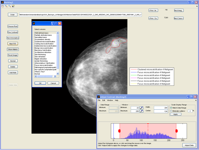
Figure 4: A snapshot for a software designed and implemented in the project to be used by the consultant radiologist to mark every lesion in a mammogram. The radiologist marks accurately the outline of a lesion with entering all related information, e.g., BIRAD and histological results.

We have implemented our protocol according to which the experienced radiologist read the digital mammograms and then marked and attributed lesions on images with the aids of a software developed in the project for that purpose; Figure 4 is a snapshot of this software. Radiologist’s annotations are done manually without semi-automation of any active contour learning algorithm [e.g., 17, 18]. The marked lesions are then tagged according to the different radiology lexicons and then categorized by the radiologist according to the “Breast Imaging Reporting and Data System” (BIRADS) scoring system (Table 2). All suspicious lesions tagged by the radiologists as BIRADS 3, 4 or 5 are pathologically proven after core and vacuum needle biopsy.

Category	Indication
0	mammographic assessment is incomplete
1	negative
2	benign finding
3	probably benign finding
4	suspicious abnormality
5	highly suggestive of malignancy

Table 2: Breast Imaging Reporting and Data System (BIRADS)

1.3 Organization of Manuscript

The sequel of this manuscript is organized as follows. Section 2 is a background and a brief literature review on CAD design and assessment. It reviews the main five steps of CAD design: breast segmentation, image enhancement, mass detection, microcalcifications detection (Sec. 2.1–2.4 respectively), which are the design steps, and assessment (Sec. 2.5). Section 3 details the design steps of our method in four subsections parallel to Sec. 2.1–2.4 respectively. Section 4 details the assessment of our method, where the method accuracy is reported and compared to both the literature methods and commercial CADs. Section 5 details the system design and assessment, where a system architecture and implementation are proposed and system performance is measured. Section 6 concludes the article and discusses current and future work to complement the present article and implemented system.

2 Background and Related Work

Designing a CAD to detect cancer from digital mammography involves many steps, including: breast segmentation (or boundary detection), image enhancement (or filtering), mass detection (or mass segmentation), microcalcification detection, and finally assessment. Each of these five steps has its own literature. There are good review papers compiling this literature. E.g., [19, 20, 21, 22] provide an overview of recent advances, and a survey of image processing algorithms, used in each of the CAD design steps. [23] present some of their recent works on the development of image processing and pattern analysis techniques. [24] is a seminal work, and from our point view is one of the best review papers written in this field, in particular, and in many other fields, in general. The authors provide both a review of the algorithms of the literature and a unique comparative study of these algorithms by reproducing them and assessing them on the same dataset and benchmark. [25, 26, 27, 28, 29, 30] provide an overall review on CAD and its history from the point of view of radiology and medicine community. It is not the objective of the present paper to provide a detailed review of the field of CAD design. However, since the objective of this project is to design a complete CAD system, and hence design each of these individual five steps, a brief literature review of each of them is due in Sec. 2.1–2.5 respectively.

2.1 Segmentation

Segmentation is the first step in CAD design, where the pixels of the breast are identified from the pixels of the background. It is called, as well, boundary detection, and should not be confused with mass segmentation and detection. The task of segmenting the breast from the background of the mammogram is relatively quite easy for that the breast pixels are spatially isolated from the background, and for that their gray levels are on the upper range of the gray level scale than the pixels of the background (of course with probable some overlap of their two histograms). The majority of the literature of segmentation use histogram based methods with different variants. The simplest of those methods is global histogram separation based on Otsu’s method [31]. [32, 33] provide a good comparison among different histogram based methods and propose a more elaborate combination between histogram based methods on a hand and active contour and morphological operations on the other hand. We developed a new histogram based iterative algorithm, with Otsu’s method as its initial seed (Sec. 3.1).

2.2 Image Enhancement

Image enhancement, or noise removal and filtering, is one of the preprocessing steps before abnormality detection. Since the quality of mammography machines and their settings along with the noise associated with the mammography process differ from one setup to others, image enhancement accounts for standardizing/normalizing images as a preprocessing step before the detection algorithms. [34, 35] provide some general survey and comparative study for the different enhancement algorithms. [36, 37, 38] perform image enhancement in the wavelet space. [39, 40, 41, 42, 43, 44] perform image enhancement by contrasting the gray level of a pixel with its surrounding, and accordingly modifying it, e.g., by subtracting the noise from the breast tissue (the signal). They used variant methods to implement this idea including: Adapted Neighborhood Contrast Enhancement (ANCE), Density Weighting Contrast Enhancement (DWCE), adaptive image enhancement using first derivative and local statistics, and region-based growing methods. [45] performs local contrast enhancement by noise modeling and removal. [46] introduced a smart idea of standardizing images by Global Histogram Equalization (GHE), where the gray levels of the breast regions will be enforced to follow uniform distribution (this is our point of departure for introducing our novel method of image enhancement (Sec. 3.2)). [47] proposed a smart low-level enhancement procedure by modeling the dominating quantum noise of the X-ray procedure as a function of gray level, then correcting the gray level. They demonstrated the efficacy of this approach in detection of microcalcification.

2.3 Mass Detection

A “Mass” refers to any circumscribed lump in the breast, which may be benign or malignant. It is the most frequent sign of breast cancer. Many approaches exist in the literature for mass detection/segmentation. A simple binary taxonomy of these approaches that helps introducing our method is: region-based vs. pixel-based. However, the two approaches may overlap and some methods can subscribe to either approaches.

In region-based approach, a whole region (or object) in the image is either clustered (segmented), given a probability (score) corresponding to the likelihood of malignancy, or assigned a binary decision (marker). This is in contrast to the pixel-based approach, where each pixel is first given a score to constitute a whole score image, which is in turn post-processed. The output of the post-processing could be, as well, clustered pixels representing regions, a final score for each region, or a decision marker.

It is worth mentioning that, the Convolution Neural Network (CNN) approach, which allows for building the recent powerful Deep Neural Networks (DNN), subscribes to the pixel-based approach. This is sense the whole image is fed directly to the network, which produces a final score image. In addition, the CNN is a featureless approach, where the CNN works directly on the plain gray level of the pixels without handcrafting any features or algorithms. Even the boundary detection (Sec. 2.1) comes as a direct byproduct of the network learning process and the final detection task.

2.3.1 Region-based approach

[41, 48, 49] use region growing for mass segmentation. [50] perform mass segmentation by active contour method. [51, 52] extracts morphological feature measures of segmented masses to classify them and to improve detection accuracy.

Many other articles tried to extract useful features from mammograms by leveraging the literature of texture analysis ([53] is an early comparative study of this literature, aside from application to mammograms). [54, 46] extract features using Law’s texture filter for gradients, and other higher covariance structure filters. [55, 56] introduced their Rubber Band Straightening Transorm (RBST) that straighten (flatten) an image object to a rectangular region. Then, for the segmented mass, they constructed Spatial Gray Level Dependence (SGLD) matirx, a form of co-occurrence matrix, which describes how different values of neighbor pixels co-occur. Different variants of co-occurrence matrix exist depending on the order of statistics used in analyzing pixel values. Later, [57] introduced a smart idea to construct a map of pixel orientation that reveals probable stellate mass structure. [58, 59] elaborated on the idea and suggested their IRIS filter that extracts gradient and directional information. It is one of the most successful methods in literature of mass detection and outperforms all other methods that was reproduced in the benchmark of [24]. [60] extracted a combination of texture based features including IRIS filter, feature from co-occurrence matrix variants, and contour related features. [61] introduce a newer version of the traditional Local Binary Pattern (LBP) co-occurrence matrix. [62] extract texture features using Histogram Gradient and Gabor filter.

Other miscellaneous approaches exist; e.g., [63, 64, 65] detect speculated masses by building a model for the linear irregular structure of the boundary of these masses. [66] attacked the problem of mass detection differently; they do least square regression for a broken line model to regress the gray level intensity of pixels surrounding a particular POI (response) on the radius from that POI (predictor). [67, 68, 69, 70, 71] extract features from multi-resolution decomposition based on wavelet analysis. [72, 73, 74] use variants of Gray Level Thresholding (GLT) to suppress pixels with low probability of malignancy. This inclues, high-to-low intensity thresholding or Dual Stage Adaptive Thresholding (DSAT). Usually thresholding is combined with other morphological procedures to smooth segmented regions resulted from thresholding.

2.3.2 Pixel-based approach

[75, 76] are CNN recent attempts before the era of DNN. [77, 78] use template matching to match the surrounding region of a pixel with a predefined template of gray level distribution that “almost” has the characteristic of mass structure; then assign a matching score to this pixel. [79] learn and design the gray level distribution of templates from real masses. [80] was one of the first attempts in the literature, if not the first, to work directly at the pixel gray level with no feature handcrafting (featureless approach). The features of each pixel are the plain gray levels in the region surrounding that pixel. Then, they train a Classification and Regression Trees (CART). [81] followed the same procedure using SVM rather than CART, with modification to the postprocessing steps; (we will follow the same featureless approcah, as well, but with novel procedure (Sec. 3.3).)

Ensemble classifier, or Multi Classifier System, almost boosted results in many fields. [82] leveraged the idea of MCS and combined several mass detection algorithms to boost the detection accuracy of their final system; (we will leverage MCS as well (Sec. 3.3.2))

2.4 Microcalcification Detection

Clusters of microcalcifications are an early sign of possible cancer and are in general not palpable. Small clusters of amorphous or faint microcalcifications may be difficult to perceive. From the results of both literature and industry, it seems that microcalcification detection is much easier for CADs than mass detection.

2.4.1 Region-based

[83, 84, 85, 86, 87, 88, 89] extract features mainly from wavelet transform. [90] detect microcalcifications using morphological operations (mainly, Sobel and Canny edge detection); then they extract features from detected objects, and feed them to SVM classifier to decrease false positives. [91, 92] relies mainly on global thresholding of image histogram then they cluster the objects using either morphological operations, e.g., erosion, or $K$-means clustering. [93] build a stochastic model using random fields to model the microcalcification.

Many articles gave attention to the fact that microcalcifications are very little calcium deposits, and hence are represented by high frequency components with respect to other background tissues. [94] design two filters, one for signal (microcalcification of high frequency) enhancement and another for background suppression then obtain the difference. [95] apply the same idea but, rather, by using a Directional Recursive Median Filter (DRMF). [96] use novel texture features derived from combined Law’s texture features.

2.4.2 Pixel-based

[97] is an early attempt to use CNN. Later, the authors elaborated in [98] on the CNN architecture and enhanced the accuracy. The authors elaborated more on the approach in [99]. Instead of using the score image output of the final layer of the CNN as a final classifier, they combined it with the morphological features of microcalcification clusters to form a new set of features, which are fed to a simple LDA classifier. They report one of the most accurate results in the literature. [100] use featureless approach described above (Sec. 2.3.2) with the Support Vector Machine (SVM) but on the output image of a High-Pass Filter (HPF) rather than the image itself. The HPF is to suppress the low frequency components that cannot be a microcalcification focus. [101] follow the same route but with replacing the SVM by Relevance Vector Machine (RVM) for faster computations. Both results are similar and are two of the most accurate results in the literature, as well, for microcalcification detection.

2.5 Assessment

2.5.1 Studies, Trials, and General Issues

Since CAD should be used as a second reader that assists radiologists (hence, the word “Aided” in CAD), there are many studies and clinical trials that report how the use of CAD affects radiologists’ reading accuracy. [102, 103, 104, 105, 106, 107, 108, 109] asserts that CAD improves radiologists’ accuracy. However, [110] concludes that CAD does not improve radiologists’ accuracy. On the other extreme, [111] (a study published in the New England Journal of Medicine and introduced by [112]) concluded that CAD reduced radiologists’ accuracy! [113] shed the light on this discrepancies, where they explain that CAD improved the accuracy of junior radiologists while it slightly improved the accuracy of seniors.

[114, 115], from the Radiology community, provide a pilot view on breast cancer screening and medical assessment of imaging system and the effect of using CAD. In addition, they suggest the best practice for assessment strategy for any imaging system, including hardware, software, time measurements, ROC analysis, etc.

The accuracy of a particular CAD is measured conditionally on a particular dataset; hence, it is the average over lesion sizes, types, and breast densities available in this dataset. Therefore, conditioning on a particular lesion size, type, or breast density will produce different accuracies. [116, 117] study the impact of breast lesion size and breast density on the measured accuracy. [118] (a study published in American Journal of Roentgenol (AJR) and discussed by [119] in the same journal) studied the accuracy of one of the available commercial CADs (Image checker 3.2) to detect amorphous calcifications. They reported that the accuracy is markedly lower than previously reported for all malignant calcifications. [120] designed their CAD so that the accuracy does not vary across different datasets. They leveraged DDSM, which is acquired from 4 different institutions, to train on one institutional dataset and test on the all three remaining. They asserted that the accuracy variance of this procedure is minimal.

2.5.2 Assessment in Terms of FROC

The de facto of the field of accuracy assessment is to report the accuracy of CADs and radiologists in terms of the conventional Receiver Operating Characteristic (ROC) or, more elaborately and accurately, the localized version Free-response ROC (FROC). [121, 122, 123, 124, 125, 126, 127] are good sources for the theory of assessment in terms of ROC and FROC. It is quite important to clarify some terminologies and notations that are usually used loosely in the literature. This paves the road for the assessment in Section 4.

A case (or study) is a collection of mammograms taken for the same patient (usually four, two per side). The case may be malignant/Positive (P) or normal/Negative (N), and similarly the image or the side, depending on whether it contains a lesion marked by the radiologist and proven by biopsy or not, respectively. If a CAD/radiologist gives a mark inside the label boundary of a positive lesion, this detection is called a True Positive (TP). The True Positive Fraction (TPF), called as well sensitivity, is the ratio between the number of TP detection over the number of total positives. However, there are four levels of defining what is “positive”: case, side, view, or lesion; for each there is a corresponding definition of TPF as follows.

Definition 1 (True Positive Fraction (TPF))

For each of the following criteria, the TPF is defined as the number of:

(“per case” or “per study”)

cases truly detected (where a positive case is counted as detected if at least one lesion is detected in at least one view of at least one side of this case) normalized by the total number of positive cases.

(“per side” or “per breast”)

sides truly detected (where a positive side is counted as detected if at least one lesion is detected in at least one view of this side) normalized by the total number of positive sides.

(“per image” or “per view”)

images (views) truly detected (where a positive image is counted as detected if at least one lesion is detected in this image) normalized by the total number of positive images.

(“per label”)

labels truly detected (where a positive label is a radiologist single marking for a lesion in a single view) normalized by the total number of positive labels. This is a very aggressive assessment measure, where it accounts for several lesions in one view. In that case, a view with two lesions, where only one of them is detected will be counted as 1/2; as opposed to the “per view” assessment, where it would be counted as 1/1.

On the other hand, the specificity is measured in terms of the number of False Markers per Image (FM/Image). It is measured by counting the number of total false markers produced by the CAD on normal images normalized by the total number of normal images. A single pair of FM/Image and its corresponding TPF constitute a single Operating Point (OP) on the FROC. Then, varying the level of reading aggressiveness produces higher OPs up the curve.

2.5.3 Assessment in Terms of Other Accuracy Measures

Rather than the de facto of the field, ROC and FROC, there are other accuracy measure indices. We will just give two of them as examples. For the assessment of region based methods, where the task can be lesion segmentation, a common accuracy measure is the Intersection over Union (IoU). It is defined as the intersection (in pixels) of the true lesion and detected one normalized by their union.

For the assessment of pixel based methods, in [13] we suggested the use of the MannWhitney statistic directly on the score image before postprocessing. The AUC of a score image is defined as

$$\widehat{AUC}=\frac{1}{n_{1}n_{2}}\sum_{i=1}^{n_{1}}{\sum_{j=1}^{n_{2}}{I_{(x_{i}<y_{j})}}},\ I_{(c)}=\left\{\begin{array}[c]{ll}1,&\text{if c is true}\\ 0,&\text{if c is false}\end{array}\right.,$$ (3)

where $x$ is the set of scores of the normal region, $y$ is the set of scores of the malignant region(s), and $n_{1}$ and $n_{2}$ are the respective number of pixels. This is a measure of the separability of the two sets of scores. The closer the AUC to a value of 1 the more the separability between the two sets of scores, and hence the more accurate the classifier on this image.

3 Method: Design

In this section we detail the design steps of our CAD. Sections 3.1–3.4 discuss the four main sequential steps: breast segmentation, image enhancement, mass detection, and microcalcification detection respectively. The method assessment is deferred to Section 4.

To leverage the training dataset, as much as possible in building the algorithms, all values of tuning and complexity parameters in this design process are obtained using the Leave-One-Out Cross-Validation (LOOCV) rather than the typical 10-fold CV. This will not influence the classifier stability since, our assessment (Figure 2) measures the “conditional” accuracy, i.e., conditional on the training dataset. This is the actual CAD that will be revealed to radiologists. For elaborate discussion on the difference among the “accuracy”, “true accuracy”, “conditional accuracy”, and other versions, the reader can refer to [128, 129, 130, 131].

3.1 Segmentation

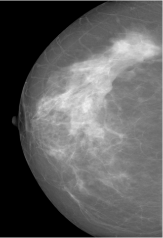
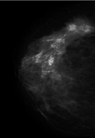
Figure 6: Image enhancement: original image (left) and the EnhancedImage (right) is both clearer for radiologists’ inspection and standardized for algorithm detection

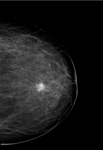
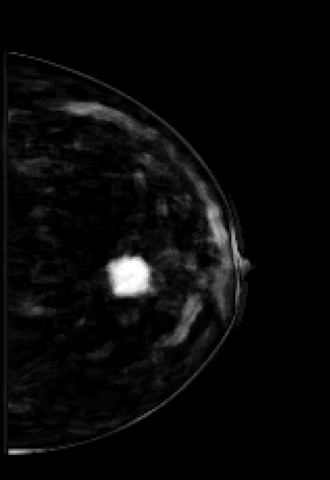
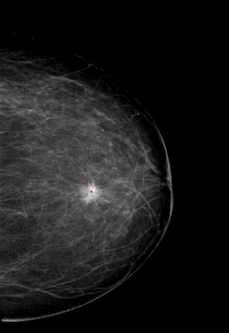
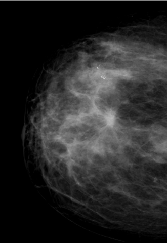
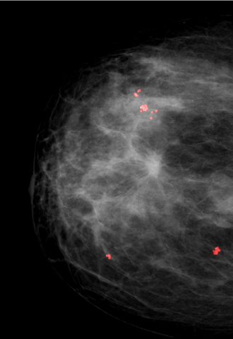
(a)                        (b)                        (c)                        (d)                        (e)

Figure 7: Output examples for mass and microcalcification detection algorithms. (a) an image containing a mass after image enhancement, (b) ScoreImage of mass detection, (c) MassLocation plotted as a red marker on the original image, (d) an image containing microcalcification, and (e) FociLocation of the detected microcalcifications plotted as red points on the original image.

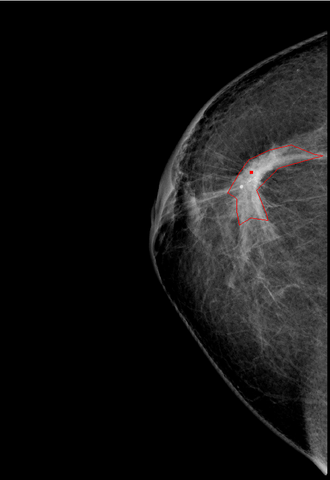
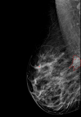
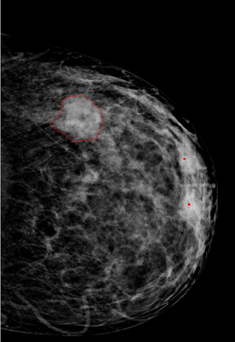
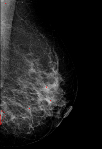
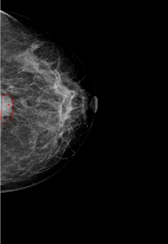
(a)                        (b)                        (c)                        (d)                        (e)

Figure 8: Mass detection examples in different mammography views; radiologist’s marking is labeled and CAD centroids of highest probability are indicated in red on each image. (a) mass detected from first centroid; (b) mass detected from second centroid with one FP; (c) mass not detected up to 2 FPs. (d) and (e) are two different views (MLO and CC respectively) of the same malignant case: (d) mass not detected up to 2 FPs; (e) mass detected from first centroid.

We do not remove the pectoral muscle since we found very few cases with lesions in it. Therefore, our segmentation algorithm starts with Otsu’s method [31] on the whole mammogram, and takes its output threshold, which classifies the image to two classes (breast and background), as an initial seed. Then, in each iteration we calculate the Quadratic Discriminant Analysis (QDA) score for each pixel in these two classes and dismiss any pixel whose QDA score and its comparison with its class mean agree. The iterative algorithm converges when the number of dismissed pixels is less than a stopping criterion that is equal to 0.002 of the total number of image pixels. The algorithm is very successful in separating the breast from the background with no overlapping region. Figures 6–8 presents examples of segmented mammograms.

3.2 Image Enhancement

Mammograms acquired from different mammography machines are of different clarity and quality for both human visual inspection and detection algorithms. Therefore, we do image enhancement in a novel way so that mammograms will look almost of the same qualitative clarity to radiologist and of the same quantitative standardization to the detection algorithms regardless of the producing mammography machine. Figure 6 is an example of the final EnhancedImage returned by the image enhancement algorithm 1 that will be explained below.

Global Histogram Equalization (GHE) is common in some literature (reviewed in Sec. 2.2); however, our novel method relies on Local Histogram Specification (LHS) as opposed to GHE or LHE. Using a sliding window, we “locally–specify” (or locally–enforce) the histogram of each pixel and its neighbors, within a vicinity, to be of a specific probability distribution with fixed chosen parameters. With this simple, yet novel, idea mammograms regardless of the producing mammography machine will have all of their pixels with the same local histogram distribution with the same parameters (it is clear that LHE is the same as LHS with Uniform distribution). We experimented with several probability densities, including Exponential, truncated Exponential, Gamma, and Uniform, we found that the exponential distribution achieves both the best visual quality and the best detection accuracy. The insight behind the exponential distribution is that it imposes more separation between the low gray level pixels and high level ones. Since cancer, whether masses or microcalcification, is depicted in mammograms as those set of pixels with higher gray level than their neighbors, the exponential distribution then helps in emphasizing this discrepancy. Quantitatively, the detection algorithm that possessed highest accuracy in terms of the FROC assessment (Sec. 4) is the exponential distribution, which supports this argument. The choice of the exponential distribution, along with the tuning parameters discussed below, are chosen using the LOOCV.

Algorithm 1 presents the steps of our image enhancement; the steps are explained as follows. As long as images come from different mammography machines, for an image $m$ we ScaleImage to a standard height of 230 pixel; the width is scaled such that the aspect ratio is preserved. We, then, SegmentImage to separate the breast from the background (Sec. 3.1). NumPixels is the BreastSize, where each of these pixels has a gray level $0\leq t<255$. For the $i\textsuperscript{th}$ pixel of interest (POI), $0\leq i<\mathtt{NumPixels}$, take a surrounding window of size $\mathtt{W}=81$ centered around $i$; this region will be of size $\mathtt{W}^{2}$ pixels and the window will be sliding to cover all POIs in the breast region (Figure 5). We do LocalHistogramSpecification of this region to set the new pixel level of the $i\textsuperscript{th}$ POI and loop over all pixels. The PDF of the window surrounding the POI, i.e., the histogram of 256 bins (a bin for each gray level value $t$) is denoted by PDFwin(t). Its Cumulative Distribution Function (CDF) is denoted by CDFwin(t). A discrete exponential density function with $\mathtt{lambda}=10$, and 256 bins as well, is created and denoted by PDFexp(t); its CDF is CDFexp(t). Now, we transform the PDF of the region surrounding the $i\textsuperscript{th}$ POI from PDFwin to PDFexp by applying the transforms of Eq. (4) to the gray levels.

$$tnew =CDFexp^{-1}\bigl{(}CDFwin(t)\bigr{)},$$ (4a)

$$CDFwin(t) =\sum_{x=0}^{x=t}PDFwin(x),$$ (4b)

$$CDFexp(t) =\sum_{x=0}^{x=t}PDFexp(x).$$ (4c)

3.3 Mass Detection

The mass detection algorithm is pixel-based and featureless (Sec. 2.3). It trains and tests (Algorithms 2–3, respectively) directly at the pixel level. Figure 7 illustrates the two outputs of these Algorithms. The figure illustrates the ScoreImage, where each pixel is assigned a score value that corresponds to its likelihood of being malignant. Therefore, high scores (bright regions) correspond to cancerous regions and low scores (black regions) correspond to normal ones. The figure illustrates as well the MassLocation, which is a red marker(s) plotted on the original image to indicate the center of a cancer.

Algorithm 2 presents the steps of the training phase. All tuning and complexity parameters discussed below are obtained using LOOCV. Each image m, where $0\leq\mathtt{m}<\mathtt{M}$, is scaled down, segmented, then enhanced using Algorithm 1. For the $i\textsuperscript{th}$ POI, $0\leq i<\mathtt{NumPixels}$, we take a surrounding window of size $\mathtt{w_{1}}=21$ (less than the $\mathtt{W}=81$ used for enhancement) centered around $i$. This region will be of size $w^{2}=441$ pixels and the window will be sliding to cover all POIs in the breast region (Figure 5). For each POI $i$, its features will be all the 441 gray levels of the surrounding window. For each training image m, the breast is divided into two regions: mass (with number of pixels $\mathtt{NumPixlesMass}$) and normal (with number of pixels $\mathtt{NumPixelsNormal}$), where of course $\mathtt{NumPixels}=\mathtt{NumPixelsMass}+\mathtt{NumPixlesNormal}$. For each image a MassFeatures matrix of size $\mathtt{NumPixelsMass}\times 441$ is constructed. Each row in this matrix represents the 441 gray levels of the surrounding window of the corresponding POI. Then a $K$-means clustering is used to obtain the best 100 representatives to reduce the number of rows; i.e., the size of the matrix will be reduced to $100\times 441$. For all training images M, the $100\times 441$ mass centroid matrix of each of them are stacked together to construct one larger matrix MassCentroidList of total size of $(100\mathtt{M}\times 441)$. Similarly, the matrix NormalCentroidList is constructed from the normal regions of the same M images. As we reduced the number of rows to find the best representatives, we reduce the number of columns (the 441 features) to find the best features. We obtain this by running Principal Component Analysis (PCA) on the $(200\mathtt{M}\times 441)$ joined matrix [MassCentroidList; NormalCentroidList], and take the largest 10 components ($\mathtt{C}=10$) to be the new reduced set of features (or PCVectors). The two matrices now are projected to the new vector space and, hence, reduced in size to $100\mathtt{M}\times 10$ each. These two matrices will be used to give a score to each pixel in a future (testing) image (Algorithm 3).

Algorithm 3 presents the steps of the testing phase. Given a testing image, the first step is to EnhanceImage (Algorithm 1). Then, for each pixel in the breast we get its 441 feature vector; this is once again the plain gray level of the pixels in a surrounding window of size $21\times 21$. This 441 feature vector is projected on the 10 PCVectors, obtained from the training phase, to produce only 10 features. Then, each pixel is compared to the two extracted matrices from the training phase, MassCentroidList and NormalCentroidList, using a KNN algorithm with chosen $\mathtt{K}=141$. The KNN algorithm gives a score to each testing pixel instead of a binary decision; the score is $\log(n_{1}/n_{2})$, where $n_{1}$ and $n_{2}$ are the number of closest training observations in each class. The global set of scores are normalized to values between 0 and 1 to be used as a probability of malignancy. After running the algorithm on all breast pixels of the testing image, this produces a ScoreImage, which will be finally post-processed to obtain the center of the cancerous mass. The post processing is the SmoothImage step. It is a mere $10\times 10$ smoothing filter that runs over the breast region of the ScoreImage. After smoothing, we search the smoothed image to FindMaxima. The location of these maxima are the MassLocation finally returned by the algorithm. The scores of these locations, ScoreImage(MassLocation), are the probability of having cancer at these locations.

Finally, when using the CAD, the radiologist can see the score image beside, or overlaying, the original image, in addition to the red marker on the cancer location (Figure 7). Radiologists can set a threshold (level of aggressiveness) to trade-off sensitivity (TPF) vs FM/Image; all centers of masses with scores lower than this level will be ignored.

3.3.1 Tuning and Complexity Parameters

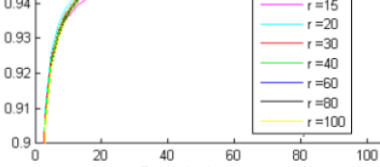
Figure 1: The plain effect—without preprocessing (enhancement) or postprocessing (score image smoothing)—of the number of centroids per image $r$ and KNN nearest neighbors $K$ on the separability of the normal and abnormal pixels measured in AUC (left) and its standard deviation (right). For each $r$, there is $K$ that is optimal in terms of the maximum AUC w.r.t. its standard deviation. The optimal $K$ increases with $r$.

As introduced above, the LOOCV was used to chose all tuning and complexity parameters just explained above: the image enhancement window size ($\mathtt{W}=81$), the exponential distribution parameter ($\mathtt{lambda}=10$), the mass detection window size ($\mathtt{w_{1}}=21$), the number of centroids per image ($\mathtt{r}=100$), the number of largest PCs ($\mathtt{C}=10$), and the KNN parameter ($\mathtt{K}=141$). For the sake of demonstration, Figure 1 illustrates the “plain effect” of the number of $K$-means clustering centroids r, which is a tuning parameter, and the number of nearest neighbors K, which is a complexity parameter, on the classifier accuracy measured in terms of the AUC (Eq. (3)) and its standard deviation. “Plain effect” means that neither preprocessing (enhancement) nor postprocessing (score image smoothing) is involved. It is clear that for a particular r, there is an optimal value of K that achieves a maximum AUC, a common phenomenon for any classifier complexity parameter. In addition, the optimal choice of K increases with r, which is expected as well since increasing r increases the final size of the data matrix. The same phenomenon happens with increasing the dataset size M for the same reason.

3.3.2 Multi Classifier System (MCS)

It is reasonable to anticipate that varying the feature window size $\mathtt{w_{1}}$ would be able to detected other masses of different size; this is a sort of detection at multi-resolution levels. An MCS version of Algorithms 2–3 is constructed by simply running it for 10 different window sizes $\mathtt{w_{1}}=6m+3,\ m=1\cdots 6$, where $\mathtt{w_{1}}=21$ is one among them. For each of these 10 windows, a score image is produced for a single mammogram; then the final score image is the average of all of these score images. The smoothing step of the final averaged score image is done as above. The MCS version increases the detection accuracy remarkably (Figure 2) as will be discussed in Sec. 4.

3.3.3 Other Classification Methods and Features

The KNN classifier was the overall winner in hundreds of experiments in which we varied classifiers and their complexity parameters. These classifiers are NN with one-layer, two-layers, and different number of neurons; SVM with different number of kernels; different versions of KNN, e.g., DANN [132, 133]; Classification and Regression Trees (CART) with varying number of parents and pruning levels; and Random Forest (RF) with varying number of trees. For each classifier, a similar behavior to that of Figure 1, is obtained. The overall winner was the KNN explained above.

In addition to various classifiers, we experimented various pixel-based methods (Sec. 2.3.2) rather than our feature-less pixel-based approach. We have reported in [13] the accuracy of the KNN classifier measured in AUC for some of these approaches including IRIS filter and template matching. Our feature-less pixel-based approach along with the KNN classifier is the overall winner among all other features and classifiers.

3.4 Microcalcification Detection

The microcalcification detection algorithm 4 detects and marks individual microcalcification foci, even if they are not clustered. Figure 7 is illustrates the output FociLocation of the microcalcification detection algorithm.

One of the well known accurate results in the literature for detecting microcalcifications, and discussed in Sec. 2.4.2, is [100]. After investigating their algorithm and reproducing their results we concluded that the naive preprocessing step, prior to the SVM training and testing, is almost what is responsible for the high accuracy—not the classification phase using the SVM. This drove our motivation to design a more sophisticated image processing step, a two-nested spatial filter, to detect the microcalcifications. So, our microcalcification detection algorithm, as opposed to the literature and as opposed to our mass detection algorithm, is based solely on image processing with no machine learning training and testing phases.

Algorithm 4 presents the steps of our algorithm of microcalcification detection. The idea of the algorithm is to detect those pixels whose very few close neighbors have high gray level, and the next surrounding neighbors have much lower level. This is essentially what characterizes the microcalcification foci. Since the size of a microcalcification focus may reach 1/1000 of the mammogram size, we scale all mammograms to a standard height of 2294 pixel, as opposed to the small scaling of 230 pixels of mass detection. The microcalcification detection algorithm scans the breast region, pixel by pixel, with sliding filter composed of two nested filters: InnerFilter (with positive coefficients and size $\mathtt{w_{2}}\times\mathtt{w_{2}}$) and OuterFilter (with negative coefficients and size $3\mathtt{w_{2}}\times 3\mathtt{w_{2}}$) as indicated in Figure 5. This filter detects the gray level contrast between high gray level POI (inner) and its low gray level surrounding neighbors (outer). The difference between these two nested filters is a measure of this contrast at each POI. In practice instead of looping on the image pixel by pixel to apply the filter we do it directly in the frequency domain using Fourier Transform for faster execution. When the contrast exceeds a particular threshold Th, the POI is a candidate microcalcification focus. As indicated in Figure 5, the boundary distance between the two filters from each side is $\mathtt{w_{2}}$, which equals to the size of InnerFilter itself. This ensures comparing the bright pixels of particular width with their surrounding neighbors of the same width. Typical chosen values, after many experimentation, are $\mathtt{w_{2}}=2$ and $\mathtt{Th}=2.4$. After applying the threshold Th we do 8-connected region to join 8-connected pixels to just a single one at their center, which will be the final mark of a single detected microcalcification focus.

A final remark on the values of the inner and outer filter (Figure 5) is due. There is only one constraint on the filter design, i.e., the summation across all of the filter pixels is zero. Since the inner filter is of size $\mathtt{w_{2}}$ and the outer filter is of size $3\mathtt{w_{2}}$, they enclose $\mathtt{w_{2}}^{2}$ and $8\mathtt{w_{2}}^{2}$ pixels respectively. Hence, the condition is $a\mathtt{w_{2}}^{2}+8b\mathtt{w_{2}}^{2}=0$, which is equivalent to $a/b=-8$. The chosen values of $1/4$ and $-1/32$, indicated in the Figure, are therefore just one possible candidate.

Finally, the following procedure is defined to cluster the detected foci. This is necessary for defining a threshold (level of aggressiveness) for the trade off between sensitivity and FM/Image, for objective assessment. The procedure starts by assigning a cluster to each individual detected focus. Then two clusters are merged together if there are two foci, one from each cluster, that are less than 3mm apart. The procedure repeats until convergence when no more cluster can be merged. Now, each cluster has a number of foci with a geometric center. The center is the final mark that is displayed as a positive finding if the number of foci in the cluster is higher than the selected threshold. If the marker gets inside the boundary of a true microcalcification cluster marked by the radiologist and proven by biopsy it is considered as a TP otherwise it is a FM.

3.5 GPU Implementation and Computational Acceleration for Algorithms and Experiments

In a project of this size, where many algorithms were tested and thousands of experiments were conducted we had to reduce the very expensive run time to acceptable bounds from a practical point of view. Three different levels of difficulties are encountered in this regard.

First, the majority of the code written for this project was in Matlab; and some codes were written in C++ for computation speedup (we reported the performance comparison between Matlab and OpenCV in [134] using 20 different datasets than the dataset of our present project). At the time of this work, MATLAB did not have the currently available OpenCL toolbox. Therefore, we wrote an opensource wrapper for MATLAB, which automated the process of compiling OpenCL kernels, converting MATLAB matrices to GPU buffers, converting data formats and, reshaping the data. This wrapper made it much easier to run, experiment, and deploy our custom kernels with a few lines of MATLAB code, and zero lines of C++ code. This wrapper is available as an opensource at [135].

Second, some algorithms were, tediously, very computationally intensive, e.g., the LHS and the KNN (3.2) since they iterate over all pixels in the dataset. Therefore, we developed GPU versions of these algorithms to take full advantage of the GPU architecture and to leverage different levels of memory and caching. The algorithm had a significant speedup of up to 120X

Third, the number of total configurations and experiments were in thousands, since it is the cross product of image enhancement parameters, feature parameters, classifier complexity parameters, etc. Therefore, We developed an in-house cluster and experiment management system; it is available, as an opensource, at [135]. At the time of this work, big data processing frameworks such as Spark and Hadoop were still infant, and did not support MATLAB. Our in-house system allowed us to operate a Beowulf cluster, run numerous experiments and have their configurations and results tracked and stored in an efficient and effective manner. Our system was akin to Sacred [136]; only it also provided provisioning and resource allocation.

4 Method: Assessment

This section reports the assessment of the mass and microcalcification detection algorithms (Sec. 3). There are three different versions of the algorithms: without LHS enhancement, with LHS enhancement, and the MCS version. For easy referencing, these three versions are denoted by LIBCAD 1, 2, and 3 respectively—the name LIBCAD is explained in Sec. 5.

On the other hand, to compare this CAD to other commercial CADs, the optimal practice is to test them all on the same dataset; this is, obviously, to have common difficulty and heterogeneity of images to avoid finite dataset size performance variance. However, comparing LIBCAD to the commercial CADs is almost impossible since it requires purchasing a license for each. Moreover, some of these commercial CADs are not deployed except with the corresponding vendor’s mammography machine. The U.S. FDA had approved the use of CADs in 1998; since then many CAD systems have been developed and approved. The literature has few published clinical trials that report the accuracy of some of these CADs. However, many of these studies report a single operating point on the FROC (a pair of sensitivity and false markers per image) of one version of a particular CAD. Moreover, not all studies report the accuracy of both mass and microcalcification detection. To the best of our knowledge, there is no comprehensive comparative study for all of these CADs. It is then very informative, even for its own sake in addition to the comparison to LIBCAD, to compile the results of all of these studies and summarize them on a single FROC; then present them along with the assessment results of LIBCAD for comparison.

Sec. 4.1 reports the assessment results of LIBCAD, Sec. 4.2 compiles the assessment results of these commercial CADs, and Figure 2 presents all of these results comparatively.

4.1 LIBCAD

Figure 2: FROCs of mass and microcalcification detection of three versions of LIBCAD, as tested on the project sequestered validation set, in comparison with the most recent U.S. FDA approved and commercial CADs (5 versions of Image Checker, 3 versions of Second Look, and AccuDetect), as appears in literature and corresponding official documents—numbers are compiled and detailed in Tables 4–5. Mass: LIBCAD 1 (and 2) are without (and with) the image enhancement via Local Histogram Specification (LHS). The effect of LHS on increasing the TPF at each FM/Image is amazing. LIBCAD 3 is the MCS version of LIBCAD 2. The effect of MCS is remarkable as well. LIBCAD 3 is slightly outperformed only by Image Checker 8 and versions above. Microcalcification: the three versions of LIBCAD have almost the same accuracy, and hence only that of LIBCAD 2 is illustrated. The figure illustrates that its sensitivity is very close to three versions of commercial CADs and highly outperforming two other versions.

4.1.1 Assessment of Mass Detection

All results are reported using a testing dataset that has never been part of the training process to avoid any overtraining. The FM/Image are obtained from testing on the normal images, whereas the sensitivity (TPF) is obtained from testing on the positive cases. Each operating point on the FROC is calculated by setting a threshold for the score of points of maxima of the final ScoreImage (Sec. 3.3). At a particular threshold, an operating point of (FM/Image, TPF) is calculated as explained in Sec. 2.5.2.

Figure 2 illustrates that the mass detection algorithm of LIBCAD 1 has the worst accuracy among others. The FROC of LIBCAD 2 is remarkably higher at all FM/Image values, and in particular at the lower range where the difference is almost 35% TPF at 0.2 FM/Image. The effect of the LHS enhancement preprocessing step is remarkable in boosting the sensitivity. LIBCAD 3 is the MCS version with LHS enhancement to enable detecting masses of different sizes. Compared to LIBCAD 2, there is a clear improvement of sensitivity at all FM/Image values. When comparing the three versions of LIBCAD to the commercial and FDA approved CADs (Sec. 4.2), it is clear that LIBCAD 1 is the worst, LIBCAD 2 has a midway sensitivity performance, whereas LIBCAD 3 achieves the highest sensitivity if compared to all others except Image Checker (ver. 8 and ver. 8.3, but not earlier versions) only at small range of FM/Image. However, at values larger than 0.5 FM/Image, no sensitivity is reported for Image Checker.

Figure 8 presents examples of true and false positives. For all displayed views, we kept decreasing the threshold until a marker appeared inside the lesion. Markers lie outside lesions are FP. The first three views are from three different cases. The last two views are from the same case. The lesion in this case is detected in one view from the first marker and not detected up to the second marker in the other view.

The TPF reported for the three versions of LIBCAD (1, 2, and 3) in Figure 2 is “per study” and only using database D1 that is explained in Table 1. Table 3 takes LIBCAD2 as an example to illustrate the behavior on different databases (D1, D2, and D3) and using different TPF assessment strategies (“per case”, “per side”, and “per image”). It is remarkable that at the mid and upper range of the FROC (FM/image of 0.85 and 1.5), the TPF is almost constant across databases, which asserts the effect of the LHS enhancement method that standardizes the probability distribution of the images. Yet, at the lower scale of the FROC (FM/image of 0.2) there is a TPF difference up to only 10%.

	D1			D2			D3
FM/image	0.2	0.85	1.5	0.2	0.85	1.5	0.2	0.85	1.5
TP Per Case	81.25	90	97	78	91.4	94	73	89	90
TP Per Side	82.4	91.2	97	76.2	90.5	93	71.5	87.5	91.2
TP Per Image	70	91.25	95	66.3	87.25	90	63.3	81.7	86.75

Table 3: Operating points using different TPF measures (Definition 1) and using different databases (Table 1). The CAD sensitivity, at each FM/image, is consistent among databases.

4.1.2 Assessment of Microcalcification Detection

Although the dataset of this project contains more than 1500 cases, the number of cases with microcalcifications is only 38 cases (67 images). For this reason, along with the fact that the microcalcification detection algorithm is not a machine learning based on training-and-testing paradigm, all of these positive cases are used to estimate the sensitivity. The FM/Image is measured on the normal cases exactly as was done for the mass detection assessment. LIBCAD detects and marks microcalcification foci, even if those foci that are not clustered (Sec. 3.4). We published a detailed study of the accuracy of LIBCAD 1 compared to the expert radiologist in [15]. The study was addressing the Radiology community and did not include technical or algorithms details. Figure 2 illustrates that at 0.25 FM/Image, the sensitivity is 0.974 (=37/38; i.e., it misses just one image out of 38). At 0.07 FM/Image, the sensitivity is 0.921 (=35/38; i.e., it misses two more images). Since the missed cases for LIBCAD 1 are very few, the accuracy improvement of LIBCAD 2, with LHS, is marginal and not significant and hence omitted. From these results, it seems that microcalcification detection is much easier in detection than mass detection except in subtle cases where a microcalcification cluster is obscured by a mass in the same case. The case missed by LIBCAD 1, as reported in [15] is of this type. To study whether the LHS of LIBCAD 2 helps in detecting microcalcifications within masses, a large number of positive cases having such a combination has to be collected. Figure 7 illustrates an example of an image with subtle microcalcifications; however, was detected and marked by the CAD.

4.2 Commercial and FDA-Approved CADs

ver.	citation	mass/$\mu$	TPF	FM/Image
Image Checker, 1998
3.1	[137]	mass	0.783	0.23
3.1	[137]	$\mu$	1	0.15
3.2	[138]	mass	0.86	2.06/4
5.0A	[139]	mass	0.818	1.08/4
5.0	[138]	mass	0.84	1.4/4
5.0	[138]	mass	0.86	1.44/4
5.0	[138]	mass	0.88	2.2/4
8.0	[138]	mass	0.83	1.0/4
8.0	[138]	mass	0.86	1.2/4
8.0	[138]	mass	0.88	1.5/4
8.0	[138]	mass	0.90	2.0/4
8.0	[137]	mass	0.89	0.33
8.0	[137]	$\mu$	1	0.13
Second Look, 2002
3.4	[140]	mass	0.84	1.1
3.4	[140]	$\mu$	0.98	0.2
6.0	[139]	mass	0.609	1.41/4
7.2	[141]	mass	0.811	1.68/4
7.2	[141]	$\mu$	0.581	0.88/4
AccuDetect, 2013
4.0.1	[141]	mass	0.838	1.68/4
4.0.1	[141]	$\mu$	0.742	0.8/4
Kodak Mammography, 2004
—	[142]	mass	0.87	1.0
—	[142]	$\mu$	0.97	1.0
Image Intelligence, —
MV-SR6577EG	[143]	mass	0.83	2.5/4
MV-SR6577EG	[143]	$\mu$	1	0.19

Table 4: Some operating points (FROC sensitivity vs. false markers per image) of 5 commercial and/or FDA-approved CADs as compiled and summarized from literature. The year following the CAD name, e.g., “Image Checker, 1998”, is the FDA approval year as appears on the FDA official site. Each row shows: a particular CAD version (ver.), the clinical trial of this CAD version (citation), type cancer detected (mass/$\mu$), sensitivity (TPF), and False Markers per Image (FM/Image). Table 5 includes comments and more details on these clinical trials. These operating points are plotted on Figure 2.

Citation	#cases	#masses	#$\mu$-calc	#mixed	#normal
[137] a	130	46	84	—	130
[138] b	—	—	—	—	—
[139]	192	192	0	0	51
[140]	201	122	54	25	155
[141]	117	85	6	26	209
[142] c	394	262	172	40	194
[143] d	208	47	38	—	123

• The 130 normal cases are the same as the 46 + 84 masses and $\mu$-calc cases; however the normal breast is used.

• It is not clear how many cases are used in this trial.

• seems to be overall accuracy.

• it seems that the in-text reported accuracy and the FROC reported in that article do not agree.

Table 5: Information and important comments on the clinical trials that reported the accuracy of the commercial and FDA-approved CADs (summarized in Table 4). Each row shows: the clinical trial (citation) and number of all cases: cases with only masses, cases with only microcalcifications, cases with both masses and microcalcifications, and normal cases (respectively). The footnotes include important comments on these trials and on their reported accuracies.

The assessment results of five of the commercial CADs are compiled from several studies and summarized in Tables 4–5, then visualized in the FROC of Figure 2. Four of these CADs are FDA approved (Image Checker, 1998; Second Look, 2002; AccuDetect, 2013; and Kodak Mammography, 2004), and the fifth is Image Intelligence. Some of these CADs are included in more than one study. Also, some different versions of the same CAD may be included in different studies. Table 4 summarizes this information along with the reported accuracies. The columns of this table present: the particular CAD version (ver.), the reporting clinical study (citation), the abnormality detected (mass/$\mu$), the sensitivity (TPF), and the corresponding specificity (FM/Image). Some of the CAD versions have one operating point appeared in one study and others have several operating points appeared collectively in different studies, hence constituting an FROC (Figure 2). Some TPF and FM/Image numbers in this table are not stated explicitly in their corresponding studies; hence we calculated them and presented them explicitly in the table. E.g., some studies reported the absolute number of detected and missed cases and absolute number of false markers (not ratios or fractions); others reported false markers per case (not FM/Image) and hence we divide by 4 (the number of views per case). The TPF in this table is “per case” (Sec. 2.5). All of these studies consider cases with only one lesion, and abandon other cases to ease calculations. This means that each case has a single lesion in one breast (side). Therefore, these “per case” results are the same as the “per side” ones.

Table 5 provides more details to the clinical studies cited in Table 4. The columns of this table present: the study (citation), total number of positive and normal cases (# cases), number of cases with masses (# masses), number of cases with microcalcifications (# $\mu$-calc), number of cases with both abnormalities (# mixed), and number of normal cases (# normal). Some important comments on these studies, concerning their results and calculation, are placed at the table footnotes.

5 System: Design and Assessment

As was introduced in Sec. 1, commercial CADs are machine dependent; i.e., deployed and connected to a particular mammography machine. On the other hand, literature is full of algorithms with no practical procedure of deploying them for public use. In this section, we propose, implement, and assess a system architecture for deploying LIBCAD to cloud. This system architecture, along with the method of image enhancement (LHS of Sec. 3.2) that makes LIBCAD suitable for mammograms from any mammography machine, may participate in spreading CAD technology.

5.1 System Design

Figure 3: System architecture for LIBCAD deployment to provide ubiquitous accessibility. The three different deployment forms (Windows DLL, Linux SO, and cloud API) are shown in red. The first two forms, i.e., DLL and SO, are deployed directly from compiled algorithms; both call the OpenCL library for speeding up computations on GPUs. The cloud-based API calls either DLL or SO (depending on the OS of the cloud machine) through a wrapper. The wrapper is C# or C++ for windows DLL or Linux SO respectively. One use of the API will be mere direct calls by developers through HTTP requests. The other use of the API could be a complete cloud-based CAD (WEBCAD) for end-users for ubiquitous accessibility (Sec. 5).

The main blocks of the system architecture are depicted in Figure 3 and explained below:

DLL or SO:

all LIBCAD algorithms are compiled to a callable library; hence the name LIBCAD (for LIBrary based CAD). The library is Dynamic Link Library (DLL) or Shared Object (SO) depending on whether the hosting machine is Windows or Linux, respectively. The importance of this step is that it makes the CAD functionalities independent of both the implementation and calling languages.

OpenCL:

This is an implementation layer of some basic and low-level computational routines to be able to run the DLL (or SO) on GPU. The importance of this layer is that it allows for fast processing necessary for some CAD functionalities, e.g., LHS of enhancement step; and allows, as well, for concurrent multiple users for higher level cloud-based access.

API:

This is a cloud-based Application Programming Interface (API) that is able to establish communication between the library (DLL or SO) and the internet external world. This API is implemented solely using PHP and we made it available as an opensource repository [135]. One way of using this API is a direct call by developers through HTTP requests, using any programming language, to integrate the CAD functionalities to their software. This software may range from simple image viewer to a sophisticated batch processing for research purposes. The other use of this API can be a full web-based CAD system (WEBCAD) for end users, e.g., radiologists.

Wrappers:

This is either C# or C++ interface layer to the DLL or SO library respectively. This wrapper is necessary to communicate with the PHP layer of the cloud-based API.

Moving CAD to cloud using the proposed architecture (Figure 3) raises other software engineering aspects and concerns. E.g., users (either programmers calling the API or end users using the WEBCAD) will need to upload their mammograms to the cloud. This is in contrast to the scenario where CADs are deployed to local mammography machines. This change of scenario comes with challenges. For instance, the DLL (or SO) libraries require a physical path to load images and temporarily storing them until the end of image analysis. To address that, we have utilized a session-based storage approach, where users upload their input images only once; these images are stored on the server for DLL (or SO) functions to access them, and are discarded after the end of each session to conserve memory and storage. However, uploading images adds an overhead, as it depends on the user’s internet speed which may vary in different parts of the world.

5.2 System Assessment

	Execution time:
Hardware Configuration	C#	DLL	PHP	Total
Image Enhancement
2 Cores / 3.5 RAM / 2.09 GHz	9.1	3.4	1.1	13.6
4 Cores / 7 RAM / 2.09 GHz	9	3	1.1	13.1
8 Cores / 14 RAM / 2.10 GHz	8.8	2.9	0.5	12.2
Mass Detection
2 Cores / 3.5 RAM / 2.09 GHz	9.2	57.6	1.4	68.2
4 Cores / 7 RAM / 2.09 GHz	8.9	31.7	1.3	41.9
8 Cores / 14 RAM / 2.10 GHz	8.9	18.7	1.5	29.1
Microcalcification Detection
2 Cores / 3.5 RAM / 2.09 GHz	2.2	16.4	1.6	20.2
4 Cores / 7 RAM / 2.09 GHz	2.1	13.8	0.9	16.8
8 Cores / 14 RAM / 2.10 GHz	2.2	13.4	1.4	17

Table 6: Execution time of each block of system architecture of Figure 3 (wrapper, DLL/SO, PHP, and total) under different hardware configurations (2, 4, 8, cores) for the three CAD functionalities (image enhancement, mass detection, and microcalcification detection).

We optimized the deployed libraries (DDL and SO), as well as, the PHP interface of the API to utilize the GPU and the multi-core architecture of the hardware. Table 6 is a benchmark that illustrates the execution time of each block of the architecture in Figure 3 and how the CAD utilizes the hardware architecture. It is clear that the majority chunk of time is consumed in the heavy computations by the main major CAD functionalities (image enhancement, mass detection, and microcalcification detection) not the wrapper nor the PHP layer. This supports the claim of the efficiency of this system architecture.

As operations are conducted online other software engineering concerns are raised, e.g., the need for advanced security measures become vital to ensure protection of data and transactions. The measures include establishing secure connections and SSL certificates. These issues are out of scope of our present article and will be discussed in another software engineering related publication.

6 Conclusion, Discussion, and Future Work

This paper is the main publication of a project coined to design a complete Computer Aided Detection (CAD) for detecting breast cancer from mammograms. The project involved several researchers from several disciplines and a large database was acquired from two different institutions for design and assessment. This CAD is complete since it is comprised of both method and system. The method is a set of algorithms designed for image enhancement, mass detection, and microcalcification detection. The system is an implementation and deployment of a software architecture that facilitates both local and cloud access to the designed algorithms so that the CAD is not limited to a particular or local mammography machine. The assessment results of both the method and the system are presented. The results of method assessment illustrate that the CAD sensitivity is much higher than the majority of commercial and FDA approved CADs. The results of system assessment illustrates that the layer responsible for deploying the CAD to the cloud has a minimal effect on the CAD performance, and that the majority of the delay comes from the algorithm computations. Phase II of the project is just launched to consider Deep Neural Networks as the method of learning for both mass and microcalcification detection. Phase III is still under planing which will consider detection of other types of abnormalities. These two phases are explained next.

6.1 Current Work: DNN and publicly available dataset

As was introduced in Section 2, a very early attempt to use CNN, which belongs to the featureless pixel-based approach, in mass and microcalcification detection was [75, 76, 97]. Since then, more than 20 years, the era of DNN evolved dramatically in both directions: DNN architecture and GPU computational power. Recent attempts to use DNN for the problem of breast cancer detection are [144, 145, 146, 147, 148, 149, 150, 151, 152]. We just launched a research project to redesign the three algorithms of image enhancement, mass detection, and microcalcification detection using DNN. We hope to come up with an architecture that wins over the designed algorithms explained in the present article. However, it is of high interest to know whether a smart DNN architecture would be able to beat the LHS algorithm designed for image enhancement? The motivation, explained in Section 3.2, behind the design of LHS was founded on the experience gained from understanding the nature of mammograms. Then the previous question may be reduced to what is the combination of the dataset size and DNN architecture that is able to win over our understanding of the nature of mammograms. Another current interest to amend this project is to document and publish the acquired datasets (Table 1) to be publicly available for the research community for future investigations.

6.2 Future Work: other types of abnormalities

There is a scientific debate whether the ethnicity of the training and testing datasets affect the CAD accuracy. Provided that the CAD of the present article is trained and tested on Egyptian dataset acquired from two different institutions, it is of great importance to us to investigate whether the accuracy would differ when testing the CAD on other datasets with different ethnicity. A parallel interesting study is to stratify the CAD accuracy for lesion size, which is akin to [116, 117].

Another track of future research is to extend CAD capabilities to detect other types of abnormalities or cancer, e.g., architectural distortion as pursued in [153, 154, 155, 156, 157, 158] or bilateral asymmetry as pursued in [159, 160, 161, 162, 163, 164, 165, 166, 167]. However, we think that detecting this kind of abnormalities is a real challenge for DNN for that the incident rate of this type of abnormalities in the diseased population is quite small if compared to mass or microcalcification. Hence, there is no enough dataset for DNN to learn from, and it seems that feature handcrafting is inevitable.

7 Acknowledgment

Many parties and individuals have contributed to this large scale project over the span of more than 5 years. The authors gratefully acknowledge the support of:

• Information Technology Industry Development Agency (ITIDA: http://www.itida.gov.eg) for funding an early stage (the first year) of this project under the grant number ARP2009.R6.3.

• MESC for Research and Development (http://www.mesclabs.com) for amending the fund of this project

• The National Campaign for Breast Cancer Screening (institution A) for providing their large datasets of mammograms.

• Alfa Scan (institution B), http://www.alfascan.com.eg, for providing their large datasets of mammograms.

• NVIDIA Corporation with the donation of the two Titan X Pascal GPU to be used for phase II of the project to redesign the CAD using DNN.

8 Appendix

Algorithm 1: EnhanceImage: image enhancement on a single image m

⬇

1EnhanceImage(m){

2 EnhancedImage=0;

3 W=81; //width of LH sliding window

4 lambda=10; //Exp dist. parameter

5 m=ScaleImage(m, 230); //standardize image height

6 m=SegmentImage(m); //segment breast from bkgrnd

7 NumPixels=BreastSize();

8 for(i=0; i < NumPixels; i++)

9 EnhancedImage(i) = LocalHistogramSpecification(m, i, W, Exp, lambda); // LHS (below)

10 return EnhancedImage;

11}

12LocalHistogramSpecification(m, i, W, Exp, lambda){

13 PDFwin = HistogramBins(m(i,W), 255); //initialize 256-bin hist. for window W surrounding POI i

14 PDFexp = HistogramBins(Exp, lambda, 255); //create 256-bin hist. for Exp(10) dist.

15 for(t=0; t<256; t++){// Calculate CDF from PDF

16 CDFwin(t)=sum(PDFwin, 0, t); //Eq. (2)

17 CDFexp(t)=sum(PDFexp, 0, t); //Eq. (3)

18 }

19 tnew=CDFexp^{-1}(CDFwin(m(i))); //Eq. (1)

20 return tnew;

21}

Algorithm 2: TrainingMassAlgorithm: training using $M$ images

⬇

1TrainingMassAlgorithm(TrainingDataset){

2 M=length(TrainingDataset); //number of training images

3 MassCentroidList = {}; //mass centroids

4 NormalCentroidList = {}; //normal centroids

5 w_1=21; //size of feature window for POI i

6 for(m=0; m < M; m++){

7 m=EnhanceImage(m);

8 MassFeatures = ConstructFeatures(m, w_1, MASS); //a NumPixelMass x 441 list to collect all pixels (NumPixelsMass) marked by radiologist as cancerours Mass and construct for each pixel the 441 features

9 NormalFeatures = ConstructFeatures(m, NORMAL); //a list of NumPixelNormal x 441 to collect all pixels (NumPixelsNormal) NOT marked by radiologist as concourse and construct for each pixel the 441 features

10 Append(Kmeans(MassFeatures, 100), MassCentroidList); //Kmeans on mass region to extract on ly 100 representatives and append them to MassCentroidList

11 Append(Kmeans(NormalRegion, 100), NormalCentroidList); //Kmeans on normal region to extract only 100 representatives and append them to NormalCentroidList

12 }

13 PCVectors = PCA([NormalCentroidList, MassCentroidList], 10); //to find the first 10 principal components of all centroids

14 [NormalCentroidList, MassCentroidList] = [MassCentroidList, NormalCentroidList] * PCVectors; //projects each of the centroid list on the best 10 PCAs to produce the two final lists of

15 centroids for cancer and normal, each is 100M x 10

16 return MassCentroidList, NormalCentroidList, PCVectors;

17}

Algorithm 3: TestingMassAlgorithm: testing on an image m

⬇

1MassDetection(m){

2 m = EnhanceImage(m);

3 ScoreImage=zeros(size(m)); //Initialize a final score image of the same original mammogram size

4 MassLocation = {}; //Initialize a final mass location list

5 NumPixels = BreastSize(m);

6 Features = ConstructFeatures(m, w_1, ALL); //A list of NumPixels x 441, where each row is the 441 gray level of the surrounding w_1xw_1 window

7 Features = Features * PCVectors; //project the NumPixels x 441 Features on the PC vectors obtained from the training phase to produce a feature list of NumPixels x 10

8 for(i=0; i < NumPixels; i++){

9 ScoreImage(i) = KNN(Features(i), NormalCentroidList, MassCentroidList); //Classify the 10-dimensional feature vector of the ith POI using a KNN classifier w.r.t. the two centroids lists obtained from training phase

10 }

11 ScoreImage = SmoothImage(ScoreImage, 10); //Smoothing by a running 10 x 10 smoothing window

12 MassLocation = FindMaxima(ScoreImage); //The locations of the potential cancers; the probability of being cancer is ScoreImage(MassLocation)

13 return ScoreImage, MassLocation;

14}

Algorithm 4: MicrocalcificationDetection algorithm on an image m

⬇

1MicrocalcificationDetection(m){

2 m = EnhanceImage(m);

3 Th = 2.4;

4 w_2 = 2;

5 FociLocation = zeros(size(m)); //Initialize a final binary image of the same size of the original mammogram to indicate the location of microcalcification foci

6 CreateFilter(InnerOuterFilter, w_2, 3 w_2); //create the filter of Figure 2

7 FociLocation = FilterImage(m, InnerOuterFilter); //to select those pixels close to each others

8 FociLocation = BW(FociLocation, Th); //With threshold Th, Convert FociLocation to B/W image

9 FociLocation = CenterOfConnectedPixels(FociLocation); //the center of each group of connected pixels is the final focus

10 return FociLocation;

11}

(a) (b)

Figure 5: The main steps of EnhanceImage and MassDectection Algorithms. (a) An image is reduced in size to 230-pixel height. Then the breast is segmented from the background. For each pixel (POI) in the breast region, a surrounding window of size 81$\times$81 is used for local histogram specification to find the new gray level of this POI. Mass detection is pursued after histogram specification using another sliding window of size 21$\times$21 centered around each POI, where its features will be a vector of the whole 21$\times$21 gray levels. (b) Filter of microcalcification detection is composed of two nested filters: inner of size $\mathtt{w2}\times\mathtt{w2}$ and outer of size $3\mathtt{w2}\times 3\mathtt{w2}$, where $\mathtt{w2}$ is chosen to be 2 pixels.

References

- [1] W. A. Yousef, Method and system for image analysis to detect cancer, patent pending, US 62/531,219 (07 2017).
- [2] M. D. Althuis, J. M. Dozier, W. F. Anderson, S. S. Devesa, L. A. Brinton, Global Trends in Breast Cancer Incidence and Mortality 1973-1997, Int. J. Epidemiol. 34 (2) (2005) 405–412 (2005).
- [3] L. S. Freedman, B. K. Edwards, L. A. G. Ries, J. L. Young, Cancer Incidence in Four Member Countries (Cyprus, Egypt, Israel, and Jordan) of the Middle East Cancer Consortium (MECC) Compared with US SEER. (2006).
- [4] L. Tabar, S. W. Duffy, B. Vitak, H. H. Chen, T. C. Prevost, The Natural History of Breast Carcinoma: What Have We Learned From screening?, Cancer 86 (3) (1999) 449–462 (1999).
- [5] T. J. Anderson, F. E. Alexander, P. M. Forrest, The Natural History of Breast Carcinoma: What Have We Learned From screening?, Cancer 88 (7) (2000) 1758–1759 (2000).
- [6] J. Ferlay, F. Bray, P. Pisani, D. M. Parkin, GLOBOCAN 2002: Cancer Incidence, Mortality and Prevalence Worldwide. (2004).
- [7] D. M. Parkin, F. Bray, J. Ferlay, P. Pisani, Global Cancer Statistics, 2002, Ca-a Cancer Journal for Clinicians 55 (2) (2005) 74–108 (2005).
- [8] R. M. Kamal, N. M. Abdel Razek, M. A. Hassan, M. A. Shaalan, Missed Breast Carcinoma; Why and How To avoid?, J Egypt Natl Canc Inst 19 (3) (2007) 178–194 (2007).
- [9] S. Radhika, Imaging Techniques Alternative To Mammography for Early Detection of Breast cancer, TRCT (2005) 1–120 (2005).
- [10] R. F. Wagner, S. V. Beiden, G. Campbell, C. E. Metz, W. M. Sacks, Assessment of Medical Imaging and Computer-Assist Systems: Lesson From Recent Experience, Acad Radiol 9 (2002) 1264–1277 (2002).
- [11] M. Muttarak, S. Pojchamarnwiputh, B. Chaiwun, Breast Carcinomas: Why Are They missed?, Singapore Med J 47 (10) (2006) 851–857 (2006).
- [12] V. M. Rao, D. C. Levin, L. Parker, B. Cavanaugh, A. J. Frangos, J. H. Sunshine, How Widely Is Computer-Aided Detection Used in Screening and Diagnostic mammography?, Journal of the American College of Radiology : JACR 7 (10) (2010) 802–5 (oct 2010).
- [13] W. a. Yousef, W. a. Mustafa, A. a. Ali, N. a. Abdelrazek, A. M. Farrag, On Detecting Abnormalities in Digital mammography, 2010 IEEE 39th Applied Imagery Pattern Recognition Workshop (AIPR) (2010) 1–7 (oct 2010).
- [14] N. M. Abdel Razek, W. A. Yousef, W. A. Mustafa, Microcalcification detection with and without prototype cad system (libcad): a comparative study, in: European Society of Radiology, ECR 2012 / C-1063, 2012, pp. 1–15 (2012).
- [15] N. M. Abdel Razek, W. A. Yousef, W. A. Mustafa, Microcalcification Detection With and Without Cad System (LIBCAD): a Comparative study, The Egyptian Journal of Radiology and Nuclear Medicine 44 (2) (2013) 397–404 (2013).
- [16] A. Jalalian, S. Mashohor, R. Mahmud, B. Karasfi, M. I. B. Saripan, A. R. B. Ramli, Foundation and methodologies in computer-aided diagnosis systems for breast cancer detection, EXCLI journal 16 (2017) 113 (2017).
- [17] Y. Zhao, J. Zhang, H. Xie, S. Zhang, L. Gu, Minimization of annotation work: Diagnosis of mammographic masses via active learning, Physics in Medicine & Biology 63 (11) (2018) 115003 (2018).
- [18] Y. Zhao, D. Chen, H. Xie, S. Zhang, L. Gu, Mammographic image classification system via active learning, Journal of Medical and Biological Engineering (2018) 1–14 (2018).
- [19] H. D. Cheng, X. P. Cai, X. W. Chen, L. M. Hu, X. L. Lou, Computer-Aided Detection and Classification of Microcalcifications in Mammograms: a survey, Pattern Recognition 36 (12) (2003) 2967–2991 (2003).
- [20] H. D. Cheng, X. J. Shi, R. Min, L. M. Hu, X. P. Cai, H. N. Du, Approaches for Automated Detection and Classification of Masses in mammograms, Pattern Recognition 39 (4) (2006) 646 (2006).
- [21] J. Bozek, M. Mustra, K. Delac, M. Grgic, A Survey of Image Processing Algorithms in Digital Mammography 631–657
- [22] J. S. Tang, R. M. Rangayyan, J. Xu, I. El Naqa, Y. Y. Yang, Computer-Aided Detection and Diagnosis of Breast Cancer With Mammography: Recent Advances, IEEE Transactions on Information Technology in Biomedicine 13 (2) (2009) 236–251 (2009).
- [23] R. M. Rangayyan, F. J. Ayres, J. E. L. Desautels, A Review of Computer-Aided Diagnosis of Breast Cancer: Toward the Detection of Subtle signs, Journal of the Franklin Institute-Engineering and Applied Mathematics 344 (3-4) (2007) 312–348 (2007).
- [24] A. Oliver, J. Freixenet, J. Marti, E. Perez, J. Pont, E. R. E. Denton, R. Zwiggelaar, A Review of Automatic Mass Detection and Segmentation in Mammographic images, Medical Image Analysis 14 (2) (2010) 87–110 (2010).
- [25] D. D. Adler, R. L. Wahl, NEW Methods for Imaging the Breast - Techniques, Findings, and POTENTIAL, American Journal of Roentgenology 164 (1) (1995) 19–30 (1995).
- [26] M. Giger, H. MacMahon, Image Processing and Computer-Aided diagnosis, Radiologic Clinics of North America 34 (3) (1996) 565–+ (1996).
- [27] C. J. Vyborny, M. L. Giger, R. M. Nishikawa, Computer-Aided Detection and Diagnosis of Breast cancer, Radiologic Clinics of North America 38 (4) (2000) 725–+ (2000).
- [28] V. Singh, C. Saunders, L. Wylie, A. Bourke, New Diagnostic Techniques for Breast Cancer detection, Future Oncology 4 (4) (2008) 501–513 (2008).
- [29] M. L. Giger, H. P. Chan, J. Boone, Anniversary Paper: History and Status of Cad and Quantitative Image Analysis: the Role of Medical Physics and AAPM, Medical Physics 35 (12) (2008) 5799–5820 (2008).
- [30] M. Elter, A. Horsch, CADx of Mammographic Masses and Clustered Microcalcifications: a review, Med Phys 36 (6) (2009) 2052–2068 (2009).
- [31] N. Otsu, A threshold selection method from gray-level histograms, IEEE transactions on systems, man, and cybernetics 9 (1) (1979) 62–66 (1979).
- [32] T. Ojala, J. Nappi, O. Nevalainen, Accurate Segmentation of the Breast Region From Digitized mammograms, Computerized Medical Imaging and Graphics 25 (1) (2001) 47–59 (2001).
- [33] R. J. Ferrari, A. F. Frère, P. R. M. Rangayyan, J. E. L. Desautels, R. A. Borges, Identification of the breast boundary in mammograms using active contour models, Medical and Biological Engineering and Computing 42 (2004) 201–208 (2004).
- [34] R. Sivaramakrishna, N. A. Obuchowski, W. A. Chilcote, G. Cardenosa, K. A. Powell, Comparing the Performance of Mammographic Enhancement Algorithms: a Preference study, American Journal of Roentgenology 175 (1) (2000) 45–51 (2000).
- [35] S. Singh, K. Bovis, An Evaluation of Contrast Enhancement Techniques for Mammographic Breast masses, IEEE Transactions on Information Technology in Biomedicine 9 (1) (2005) 109–119 (2005).
- [36] P. Sakellaropoulos, L. Costaridou, G. Panayiotakis, A Wavelet-Based Spatially Adaptive Method for Mammographic Contrast enhancement, Physics in Medicine and Biology 48 (6) (2003) 787–803 (2003).
- [37] J. Scharcanski, C. R. Jung, Denoising and Enhancing Digital Mammographic Images for Visual screening, Computerized Medical Imaging and Graphics 30 (4) (2006) 243–254 (2006).
- [38] J. Tang, S. Qingling, K. Agyepong, An Image Enhancement Algorithm Based on a Contrast Measure in the Wavelet Domain for Screening Mammograms, in: Image Processing, 2007. ICIP 2007. IEEE International Conference on, Vol. 5, 2007, pp. V – 29–V – 32 (2007).
- [39] A. P. Dhawan, G. Buelloni, R. Gordon, Enhancement of Mammographic Features By Optimal Adaptive Neighborhood Image Processing, Medical Imaging, IEEE Transactions on 5 (1) (1986) 8–15 (1986).
- [40] W. M. Morrow, R. B. Paranjape, R. M. Rangayyan, J. E. L. Desautels, REGION-BASED Contrast Enhancement of MAMMOGRAMS, IEEE Transactions on Medical Imaging 11 (3) (1992) 392–406 (1992).
- [41] N. Petrick, H. P. Chan, B. Sahiner, D. T. Wei, M. A. Helvie, M. M. Goodsitt, D. D. Adler, Automated Detection of Breast Masses on Digital Mammograms Using Adaptive Density-Weighted Contrast Enhancement Filtering, Medical Imaging 1995: Image Processing 2434 (1995) 590–597 (1995).
- [42] N. Petrick, H. P. Chan, B. Sahiner, D. T. Wei, An Adaptive Density-Weighted Contrast Enhancement Filter for Mammographic Breast Mass detection, IEEE Transactions on Medical Imaging 15 (1) (1996) 59–67 (1996).
- [43] R. M. Rangayyan, L. Shen, Y. Shen, J. E. Desautels, H. Bryant, T. J. Terry, N. Horeczko, M. S. Rose, Improvement of Sensitivity of Breast Cancer Diagnosis With Adaptive Neighborhood Contrast Enhancement of mammograms, IEEE transactions on information technology in biomedicine : a publication of the IEEE Engineering in Medicine and Biology Society 1 (3) (1997) 161–170 (1997).
- [44] J. K. Kim, J. M. Park, K. S. Song, H. W. Park, Adaptive Mammographic Image Enhancement Using First Derivative and Local statistics, IEEE Transactions on Medical Imaging 16 (5) (1997) 495–502 (1997).
- [45] W. J. Veldkamp, N. Karssemeijer, Normalization of Local Contrast in mammograms, IEEE Trans Med Imaging 19 (7) (2000) 731–738 (2000).
- [46] R. Gupta, P. E. Undrill, The Use of Texture Analysis To Delineate Suspicious Masses in Mammography, Physics in Medicine and Biology 40 (5) (1995) 835–855 (1995).
- [47] K. J. McLoughlin, P. J. Bones, N. Karssemeijer, Noise Equalization for Detection of Microcalcification Clusters in Direct Digital Mammogram images, IEEE Transactions on Medical Imaging 23 (3) (2004) 313–320 (2004).
- [48] N. Petrick, H. P. Chan, D. T. Wei, B. Sahiner, M. A. Helvie, D. D. Adler, Automated Detection of Breast Masses on Mammograms Using Adaptive Contrast Enhancement and Texture classification, Medical Physics 23 (10) (1996) 1685–1696 (1996).
- [49] N. Petrick, H. P. Chan, B. Sahiner, M. A. Helvie, Combined Adaptive Enhancement and Region-Growing Segmentation of Breast Masses on Digitized mammograms, Med Phys 26 (8) (1999) 1642–1654 (1999).
- [50] M. Ciecholewski, Malignant and benign mass segmentation in mammograms using active contour methods, Symmetry 9 (11) (2017) 277 (2017).
- [51] R. M. Rangayyan, N. M. El-Faramawy, J. E. Desautels, O. A. Alim, Measures of Acutance and Shape for Classification of Breast tumors, IEEE Trans Med Imaging 16 (6) (1997) 799–810 (1997).
- [52] B. Sahiner, H. P. Chan, N. Petrick, M. A. Helvie, L. M. Hadjiiski, Improvement of Mammographic Mass Characterization Using Spiculation Meausures and Morphological features, Med Phys 28 (7) (2001) 1455–1465 (2001).
- [53] T. Ojala, M. Pietikainen, D. Harwood, A Comparative Study of Texture Measures With Classification Based on Feature distributions, Pattern Recognition 29 (1) (1996) 51–59 (1996).
- [54] D. Harwood, T. Ojala, M. Pietikainen, S. Kelman, L. Davis, Texture Classification By Center-Symmetrical Autocorrelation, Using Kullback Discrimination of Distributions, Pattern Recognition Letters 16 (1) (1995) 1–10 (1995).
- [55] H. P. Chan, D. Wei, M. A. Helvie, B. Sahiner, D. D. Adler, M. M. Goodsitt, N. Petrick, Computer-Aided Classification of Mammographic Masses and Normal Tissue: Linear Discriminant Analysis in Texture Feature space, Phys Med Biol 40 (5) (1995) 857–876 (1995).
- [56] B. Sahiner, H. P. Chan, N. Petrick, M. A. Helvie, M. M. Goodsitt, Computerized Characterization of Masses on Mammograms: the Rubber Band Straightening Transform and Texture analysis, Med Phys 25 (4) (1998) 516–526 (1998).
- [57] N. Karssemeijer, G. M. Te Brake, Detection of Stellate Distortions in mammograms, IEEE Trans Med Imaging 15 (5) (1996) 611–619 (1996).
- [58] H. Kobatake, S. Hashimoto, Convergence Index Filter for Vector fields, Ieee Transactions on Image Processing 8 (8) (1999) 1029–1038 (1999).
- [59] H. Kobatake, M. Murakami, H. Takeo, S. Nawano, Computerized Detection of Malignant Tumors on Digital mammograms, IEEE Trans Med Imaging 18 (5) (1999) 369–378 (1999).
- [60] C. Varela, P. G. Tahoces, A. J. Mendez, M. Souto, J. J. Vidal, Computerized Detection of Breast Masses in Digitized mammograms, Computers in Biology and Medicine 37 (2) (2007) 214–226 (2007).
- [61] A. Midya, R. Rabidas, A. Sadhu, J. Chakraborty, Edge weighted local texture features for the categorization of mammographic masses, Journal of Medical and Biological Engineering (2018) 1–12 (2018).
- [62] A. A. Shastri, D. Tamrakar, K. Ahuja, Density-wise two stage mammogram classification using texture exploiting descriptors, Expert Systems with Applications 99 (2018) 71–82 (2018).
- [63] R. Zwiggelaar, T. C. Parr, J. E. Schumm, I. W. Hutt, C. J. Taylor, S. M. Astley, C. R. Boggis, Model-Based Detection of Spiculated Lesions in mammograms, Med Image Anal 3 (1) (1999) 39–62 (1999).
- [64] R. Zwiggelaar, C. J. Taylor, C. M. E. Rubin, Detection of the Central Mass of Spiculated Lesions - Signature Normalisation and Model Data aspects, Information Processing in Medical Imaging, Proceedings 1613 (1999) 406–411 (1999).
- [65] R. Zwiggelaar, S. M. Astley, C. R. M. Boggis, C. J. Taylor, Linear Structures in Mammographic Images: Detection and classification, IEEE Transactions on Medical Imaging 23 (9) (2004) 1077–1086 (2004).
- [66] T. Hastie, D. Ikeda, R. Tibshirani, Statistical Measures for the Computer-Aided Diagnosis of Mammographic masses, Journal of Computational and Graphical Statistics 8 (3) (1999) 531–543 (1999).
- [67] L. H. Li, W. Qian, L. P. Clarke, Digital Mammography: Computer-Assisted Diagnosis Method for Mass Detection With Multiorientation and Multiresolution Wavelet transforms, Academic Radiology 4 (11) (1997) 724–731 (1997).
- [68] W. Qian, L. H. Li, L. P. Clarke, Image Feature Extraction for Mass Detection in Digital Mammography: Influence of Wavelet analysis, Medical Physics 26 (3) (1999) 402–408 (1999).
- [69] W. Qian, X. J. Sun, D. S. Song, R. A. Clark, Digital Mammography: Wavelet Transform and Kalman-Filtering Neural Network in Mass Segmentation and detection, Academic Radiology 8 (11) (2001) 1074–1082 (2001).
- [70] L. H. Li, R. A. Clark, J. A. Thomas, Computer-Aided Diagnosis of Masses With Full-Field Digital mammography, Academic Radiology 9 (1) (2002) 4–12 (2002).
- [71] E. A. Rashed, I. A. Ismail, S. I. Zaki, Multiresolution Mammogram Analysis in Multilevel decomposition, Pattern Recognition Letters 28 (2) (2007) 286–292 (2007).
- [72] J. Anitha, J. D. Peter, S. I. A. Pandian, A dual stage adaptive thresholding (dusat) for automatic mass detection in mammograms, Computer methods and programs in biomedicine 138 (2017) 93–104 (2017).
- [73] J. Chakraborty, A. Midya, R. Rabidas, Computer-aided detection and diagnosis of mammographic masses using multi-resolution analysis of oriented tissue patterns, Expert Systems with Applications 99 (2018) 168–179 (2018).
- [74] J. Chakraborty, A. Midya, S. Mukhopadhyay, R. M. Rangayyan, A. Sadhu, V. Singla, N. Khandelwal, Computer-aided detection of mammographic masses using hybrid region growing controlled by multilevel thresholding, Journal of Medical and Biological Engineering (2018) 1–15 (2018).
- [75] S. C. B. Lo, H. P. Chan, J. S. Lin, H. Li, M. T. Freedman, S. K. Mun, Artificial Convolution Neural Network for Medical Image Pattern recognition, Neural Networks 8 (7-8) (1995) 1201–1214 (1995).
- [76] B. Sahiner, H. P. Chan, N. Petrick, D. Wei, M. A. Helvie, D. D. Adler, M. M. Goodsitt, Classification of Mass and Normal Breast Tissue: a Convolution Neural Network Classifier With Spatial Domain and Texture images, IEEE Trans Med Imaging 15 (5) (1996) 598–610 (1996).
- [77] S. M. Lai, X. B. Li, W. F. Bischof, On Techniques for Detecting Circumscribed Masses in Mammograms, IEEE Transactions on Medical Imaging 8 (4) (1989) 377–386 (1989).
- [78] G. M. te Brake, N. Karssemeijer, Single and Multiscale Detection of Masses in Digital mammograms, IEEE Trans Med Imaging 18 (7) (1999) 628–639 (1999).
- [79] J. Freixenet, A. Oliver, R. Marti, X. Llado, J. Pont, E. Perez, E. R. E. Denton, R. Zwiggelaar, Eigendetection of Masses Considering False Positive Reduction and Breast Density information, Medical Physics 35 (5) (2008) 1840–1853 (2008).
- [80] W. P. Kegelmeyer Jr, J. M. Pruneda, P. D. Bourland, A. Hillis, M. W. Riggs, M. L. Nipper, Computer-Aided Mammographic Screening for Spiculated lesions, Radiology 191 (2) (1994) 331–337 (1994).
- [81] R. Campanini, D. Dongiovanni, E. Iampieri, N. Lanconelli, M. Masotti, G. Palermo, A. Riccardi, M. Roffilli, A Novel Featureless Approach To Mass Detection in Digital Mammograms Based on Support Vector machines, Physics in Medicine and Biology 49 (6) (2004) 961–975 (2004).
- [82] J. Y. Choi, D. H. Kim, K. N. Plataniotis, Y. M. Ro, Computer-Aided Detection (cad) of Breast Masses in Mammography: Combined Detection and Ensemble classification., Physics in medicine and biology 59 (14) (2014) 3697–719 (2014).
- [83] W. Qian, L. P. Clarke, M. Kallergi, H. D. Li, R. Velthuizen, R. A. Clark, M. L. Silbiger, Tree-Structured Nonlinear Filter and Wavelet Transform for Microcalcification Segmentation in Mammography, Biomedical Image Processing and Biomedical Visualization, Pts 1 and 2 1905 (1993) 509–520 (1993).
- [84] H. Yoshida, W. Zhang, W. D. Cai, K. N. Doi, R. M. Nishikawa, M. L. Giger, Optimizing Wavelet Transform Based on Supervised Learning for Detection of Micro Calcifications in Digital mammograms, International Conference on Image Processing - Proceedings, Vols I-Iii (1995) C152–C155 2002 (1995).
- [85] R. N. Strickland, H. I. Hahn, Wavelet Transforms for Detecting Microcalcifications in mammograms, IEEE Transactions on Medical Imaging 15 (2) (1996) 218–229 (1996).
- [86] C. H. Chen, G. G. Lee, On Digital Mammogram Segmentation and Microcalcification Detection Using Multiresolution Wavelet Analysis, Graphical Models and Image Processing 59 (5) (1997) 349–364 (1997).
- [87] S. Y. Yu, L. Guan, A Cad System for the Automatic Detection of Clustered Microcalcifications in Digitized Mammogram films, IEEE Transactions on Medical Imaging 19 (2) (2000) 115–126 (2000).
- [88] P. Heinlein, J. Drexl, W. Schneider, Integrated Wavelets for Enhancement of Microcalcifications in Digital mammography, IEEE Transactions on Medical Imaging 22 (3) (2003) 402–413 (2003).
- [89] A. N. Karahaliou, I. S. Boniatis, S. G. Skiadopoulos, F. N. Sakellaropoulos, N. S. Arikidis, E. A. Likaki, G. S. Panayiotakis, L. I. Costaridou, Breast Cancer Diagnosis: Analyzing Texture of Tissue Surrounding Microcalcifications, IEEE Transactions on Information Technology in Biomedicine 12 (6) (2008) 731–738 (2008).
- [90] S. Singh, V. Kumar, H. K. Verma, D. Singh, SVM Based System for Classification of Microcalcifications in Digital mammograms, Conf Proc IEEE Eng Med Biol Soc 1 (2006) 4747–4750 (2006).
- [91] R. M. Nishikawa, M. L. Giger, K. Doi, C. J. Vyborny, R. A. Schmidt, Computer-Aided Detection of Clustered Microcalcifications on Digital mammograms, Med Biol Eng Comput 33 (2) (1995) 174–178 (1995).
- [92] J. Ge, H. P. Chan, B. Sahiner, C. Zhou, M. A. Helvie, J. Wei, L. M. Hadjiiski, Y. Zhang, Y. T. Wu, J. Shi, Automated Detection of Breast Vascular Calcification on Full-Field Digital Mammograms - Art. No. 691517, Medical Imaging 2008: Computer-Aided Diagnosis, Pts 1 and 2 6915 (2008) 91517 (2008).
- [93] N. Karssemeijer, Stochastic-Model for Automated Detection of Calcifications in Digital Mammograms, Image and Vision Computing 10 (6) (1992) 369–375 (1992).
- [94] H. P. Chan, K. Doi, S. Galhotra, C. J. Vyborny, H. Macmahon, P. M. Jokich, Image Feature Analysis and Computer-Aided Diagnosis in Digital Radiography .1. Automated Detection of Microcalcifications in Mammography, Medical Physics 14 (4) (1987) 538–548 (1987).
- [95] E. Cernadas, R. Zwiggelaar, W. Veldkamp, T. Parr, S. Astley, C. Taylor, C. Boggis, Detection of mammographic microcalcifications using a statistical model, in: N. Karssemeijer, M. Thijssen, J. Hendriks, L. VanErning (Eds.), Digital Mammography, Vol. 13, 1998, pp. 205–208 (1998).
- [96] P. Shi, J. Zhong, A. Rampun, H. Wang, A hierarchical pipeline for breast boundary segmentation and calcification detection in mammograms, Computers in biology and medicine 96 (2018) 178–188 (2018).
- [97] H. P. Chan, S. C. B. Lo, B. Sahiner, K. L. Lam, M. A. Helvie, Computer-Aided Detection of Mammographic Microcalcifications - Pattern-Recognition With an Artificial Neural-Network, Medical Physics 22 (10) (1995) 1555–1567 (1995).
- [98] M. N. Gurcan, H.-P. Chan, B. Sahiner, L. Hadjiiski, N. Petrick, M. A. Helvie, Optimal neural network architecture selection, Academic Radiology 9 (4) (2002) 420–429 (Apr 2002).
- [99] J. Ge, B. Sahiner, L. M. Hadjiiski, H. P. Chan, J. Wei, M. A. Helvie, C. Zhou, Computer Aided Detection of Clusters of Microcalcifications on Full Field Digital mammograms, Medical Physics 33 (8) (2006) 2975–2988 (2006).
- [100] I. El-Naqa, Y. Yang, M. N. Wernick, N. P. Galatsanos, R. M. Nishikawa, A Support Vector Machine Approach for Detection of microcalcifications, IEEE Trans Med Imaging 21 (12) (2002) 1552–1563 (2002).
- [101] L. Wei, Y. Yang, R. M. Nishikawa, M. N. Wernick, A. Edwards, Relevance Vector Machine for Automatic Detection of Clustered microcalcifications, IEEE Trans Med Imaging 24 (10) (2005) 1278–1285 (2005).
- [102] H. P. Chan, K. Doi, C. J. Vyborny, R. A. Schmidt, C. E. Metz, K. L. Lam, T. Ogura, Y. Z. Wu, H. Macmahon, Improvement in Radiologists Detection of Clustered Microcalcifications on Mammograms - the Potential of Computer-Aided Diagnosis, Investigative Radiology 25 (10) (1990) 1102–1110 (1990).
- [103] H. P. Chan, B. Sahiner, M. A. Helvie, N. Petrick, M. A. Roubidoux, T. E. Wilson, D. D. Adler, C. Paramagul, J. S. Newman, S. Sanjay-Gopal, Improvement of Radiologists’ Characterization of Mammographic Masses By Using Computer-Aided Diagnosis: an Roc study, Radiology 212 (3) (1999) 817–827 (1999).
- [104] Y. Jiang, R. M. Nishikawa, R. A. Schmidt, C. E. Metz, M. L. Giger, K. Doi, Improving Breast Cancer Diagnosis With Computer-Aided diagnosis, Academic Radiology 6 (1) (1999) 22–33 (1999).
- [105] T. W. Freer, M. J. Ulissey, Screening Mammography With Computer-Aided Detection: Prospective Study of 12,860 Patients in a Community Breast center, Radiology 220 (3) (2001) 781–786 (2001).
- [106] N. Petrick, B. Sahiner, H. P. Chan, M. A. Helvie, S. Paquerault, L. M. Hadjiiski, Breast Cancer Detection: Evaluation of a Mass-Detection Algorithm for Computer-Aided Diagnosis – Experience in 263 patients, Radiology 224 (1) (2002) 217–224 (2002).
- [107] L. Hadjiiski, H. P. Chan, B. Sahiner, M. A. Helvie, M. A. Roubidoux, C. Blane, C. Paramagul, N. Petrick, J. Bailey, K. Klein, M. Foster, S. Patterson, D. Adler, A. Nees, J. Shen, Improvement in Radiologists’ Characterization of Malignant and Benign Breast Masses on Serial Mammograms With Computer-Aided Diagnosis: an Roc study, Radiology 233 (1) (2004) 255–265 (2004).
- [108] J. M. Ko, M. J. Nicholas, J. B. Mendel, P. J. Slanetz, Prospective Assessment of Computer-Aided Detection in Interpretation of Screening mammography, AJR Am J Roentgenol 187 (6) (2006) 1483–1491 (2006).
- [109] F. J. Gilbert, S. M. Astley, M. G. Gillan, O. F. Agbaje, M. G. Wallis, J. James, C. R. Boggis, S. W. Duffy, Single Reading With Computer-Aided Detection for Screening mammography, N Engl J Med 359 (16) (2008) 1675–1684 (2008).
- [110] D. Gur, J. H. Sumkin, H. E. Rockette, M. Ganott, C. Hakim, L. Hardesty, W. R. Poller, R. Shah, L. Wallace, Changes in Breast Cancer Detection and Mammography Recall Rates After the Introduction of a Computer-Aided Detection system, J Natl Cancer Inst 96 (3) (2004) 185–190 (2004).
- [111] J. J. Fenton, S. H. Taplin, P. A. Carney, L. Abraham, E. A. Sickles, C. D’Orsi, E. A. Berns, G. Cutter, R. E. Hendrick, W. E. Barlow, J. G. Elmore, Influence of Computer-Aided Detection on Performance of Screening Mammography, N Engl J Med 356 (14) (2007) 1399–1409 (2007).
- [112] F. M. Hall, Breast Imaging and Computer-Aided Detection, N Engl J Med 356 (14) (2007) 1464–1466 (2007).
- [113] C. Balleyguier, K. Kinkel, J. Fermanian, S. Malan, G. Djen, P. Taourel, O. Helenon, Computer-Aided Detection (cad) in Mammography: Does It Help the Junior Or the Senior radiologist?, Eur J Radiol 54 (1) (2005) 90–96 (2005).
- [114] K. M. Harris, V. G. Vogel, Breast Cancer screening, Cancer and Metastasis Reviews 16 (3-4) (1997) 231–262 (1997).
- [115] E. A. Krupinski, Y. L. Jiang, Anniversary Paper: Evaluation of Medical Imaging systems, Medical Physics 35 (2) (2008) 645–659 (2008).
- [116] A. Malich, D. Sauner, C. Marx, M. Facius, T. Boehm, S. O. Pfleiderer, M. Fleck, W. A. Kaiser, Influence of Breast Lesion Size and Histologic Findings on Tumor Detection Rate of a Computer-Aided Detection system, Radiology 228 (3) (2003) 851–856 (2003).
- [117] R. F. Brem, J. W. Hoffmeister, J. A. Rapelyea, G. Zisman, K. Mohtashemi, G. Jindal, M. P. Disimio, S. K. Rogers, Impact of Breast Density on Computer-Aided Detection for Breast cancer, AJR Am J Roentgenol 184 (2) (2005) 439–444 (2005).
- [118] M. S. Soo, E. L. Rosen, J. Q. Xia, S. Ghate, J. A. Baker, Computer-Aided Detection of Amorphous calcifications, AJR Am J Roentgenol 184 (3) (2005) 887–892 (2005).
- [119] F. M. Hall, Computer-Aided Detection (cad) of Amorphous calcifications, AJR Am J Roentgenol 186 (3) (2006) 902; author reply 902–3 (2006).
- [120] A. Garcia-Manso, C. J. Garcia-Orellana, H. Gonzalez-Velasco, R. Gallardo-Caballero, M. M. Macias, Consistent Performance Measurement of a System To Detect Masses in Mammograms Based on Blind Feature extraction, Biomed Eng Online 12 (2013) 2 (2013).
- [121] M. Kallergi, G. M. Carney, J. Gaviria, Evaluating the Performance of Detection Algorithms in Digital mammography, Med Phys 26 (2) (1999) 267–275 (1999).
- [122] P. Baldi, S. Brunak, Y. Chauvin, C. A. Andersen, H. Nielsen, Assessing the Accuracy of Prediction Algorithms for Classification: an overview, Bioinformatics 16 (5) (2000) 412–424 (2000).
- [123] D. P. Chakraborty, K. S. Berbaum, Observer Studies Involving Detection and Localization: Modeling, Analysis, and validation, Medical Physics 31 (8) (2004) 2313–2330 (2004).
- [124] R. F. Wagner, C. E. Metz, G. Campbell, Assessment of Medical Imaging Systems and Computer Aids: a Tutorial Review, Academic Radiology 14 (2007) 723–748 (2007).
- [125] H. J. Yoon, B. Zheng, B. Sahiner, D. P. Chakraborty, Evaluating Computer-Aided Detection algorithms, Med Phys 34 (6) (2007) 2024–2038 (2007).
- [126] X. He, E. Frey, ROC, Lroc, Froc, Afroc: an Alphabet soup, J Am Coll Radiol 6 (9) (2009) 652–655 (2009).
- [127] A. Wunderlich, F. Noo, A Nonparametric Procedure for Comparing the Areas Under Correlated Lroc Curves, IEEE Transactions on Medical Imaging 31 (11) (2012) 2050–2061 (2012).
- [128] W. A. Yousef, R. F. Wagner, M. H. Loew, Comparison of Non-Parametric Methods for Assessing Classifier Performance in Terms of {ROC} Parameters, in: Applied Imagery Pattern Recognition Workshop, 2004. Proceedings. 33rd; IEEE Computer Society, 2004, pp. 190–195 (2004).
- [129] W. A. Yousef, R. F. Wagner, M. H. Loew, Assessing Classifiers From Two Independent Data Sets Using {ROC} Analysis: a Nonparametric Approach, Pattern Analysis and Machine Intelligence, IEEE Transactions on 28 (11) (2006) 1809–1817 (2006).
- [130] W. A. Yousef, AUC: nonparametric estiamtors and their smoothness, arXiv preprint arXiv:1907.12851 (2019).
- [131] W. A. Yousef, Prudence when assuming normality: an advice for machine learning practitioners, arXiv preprint arXiv:1907.12852 (2019).
- [132] K. Fukunaga, T. E. Flick, AN Optimal Global Nearest Neighbor METRIC, Ieee Transactions on Pattern Analysis and Machine Intelligence 6 (3) (1984) 314–318 (1984).
- [133] R. D. Short, K. Fukunaga, The Optimal Distance Measure for Nearest Neighbor classification, Information Theory, IEEE Transactions on 27 (5) (1981) 622–627 (1981).
- [134] A. A. Elsayed, W. A. Yousef, Matlab vs. opencv: A comparative study of different machine learning algorithms, arXiv preprint arXiv:1905.01213 (2019).
- [135] MESC Labs, LIBCAD-OpenSource: Software Utilities for Computer Aided Detection (CAD): https://github.com/mesclabs/LIBCAD-OpenSource-Utils (2012).
- [136] K. Greff, A. Klein, M. Chovanec, F. Hutter, J. Schmidhuber, The sacred infrastructure for computational research: https://github.com/IDSIA/sacred, Proceedings of the 15th Python in Science Conference (2017) 49–56 (2017).
- [137] S. J. Kim, W. K. Moon, S. Y. Kim, J. M. Chang, S. M. Kim, N. Cho, Comparison of Two Software Versions of a Commercially Available Computer-Aided Detection (cad) System for Detecting Breast cancer, Acta Radiol 51 (5) (2010) 482–490 (2010).
- [138] J. Roehrig, The Manufacturer’s perspective, Br J Radiol 78 Spec No (2005) S41–5 (2005).
- [139] R. L. Ellis, A. A. Meade, M. A. Mathiason, K. M. Willison, W. Logan-Young, Evaluation of Computer-Aided Detection Systems in the Detection of Small Invasive Breast Carcinoma1, Radiology 245 (1) (2007) 88–94 (2007).
- [140] R. F. Brem, J. W. Hoffmeister, G. Zisman, M. P. DeSimio, S. K. Rogers, A Computer-Aided Detection System for the Evaluation of Breast Cancer By Mammographic Appearance and Lesion size, AJR Am J Roentgenol 184 (3) (2005) 893–896 (2005).
- [141] M. Lobbes, M. Smidt, K. Keymeulen, R. Girometti, C. Zuiani, R. Beets-Tan, J. Wildberger, C. Boetes, Malignant Lesions on Mammography: Accuracy of Two Different Computer-Aided Detection systems, Clinical Imaging 37 (2) (2013) 283–288 (2013).
- [142] Kodak, Kodak Mammography, CAD Engine - P030007 (2004).
- [143] Y. Kuroki, R. Sekiguchi, T. Endo, Utsonomiya/JP, T. Utsunomiya, Nagoya/JP, FujifilmCAD.pdf, in: Performance evaluation of the mammography CAD (Computer Aided Detection) on the direct conversion FPD system with a pixel size of 50m, ECR 2012 / C-0930, 2012 (2012).
- [144] G. Carneiro, J. Nascimento, A. P. Bradley, Deep learning models for classifying mammogram exams containing unregistered multi-view images and segmentation maps of lesions, in: Deep Learning for Medical Image Analysis, Elsevier, 2017, pp. 321–339 (2017).
- [145] A. Akselrod-Ballin, L. Karlinsky, A. Hazan, R. Bakalo, A. B. Horesh, Y. Shoshan, E. Barkan, Deep learning for automatic detection of abnormal findings in breast mammography, in: Deep Learning in Medical Image Analysis and Multimodal Learning for Clinical Decision Support, Springer, 2017, pp. 321–329 (2017).
- [146] A. Akselrod-Ballin, L. Karlinsky, S. Alpert, S. Hashoul, R. Ben-Ari, E. Barkan, A cnn based method for automatic mass detection and classification in mammograms, Computer Methods in Biomechanics and Biomedical Engineering: Imaging & Visualization (2017) 1–8 (2017).
- [147] Y. Qiu, S. Yan, R. R. Gundreddy, Y. Wang, S. Cheng, H. Liu, B. Zheng, A new approach to develop computer-aided diagnosis scheme of breast mass classification using deep learning technology, Journal of X-ray science and technology 25 (5) (2017) 751–763 (2017).
- [148] A. Hamidinekoo, E. Denton, A. Rampun, K. Honnor, R. Zwiggelaar, Deep learning in mammography and breast histology, an overview and future trends, Medical image analysis 47 (2018) 45–67 (2018).
- [149] N. Dhungel, G. Carneiro, A. P. Bradley, A deep learning approach for the analysis of masses in mammograms with minimal user intervention, Medical image analysis 37 (2017) 114–128 (2017).
- [150] G. Carneiro, J. Nascimento, A. P. Bradley, Automated analysis of unregistered multi-view mammograms with deep learning, IEEE transactions on medical imaging 36 (11) (2017) 2355–2365 (2017).
- [151] N. Dhungel, G. Carneiro, A. P. Bradley, Fully automated classification of mammograms using deep residual neural networks, in: Biomedical Imaging (ISBI 2017), 2017 IEEE 14th International Symposium on, IEEE, 2017, pp. 310–314 (2017).
- [152] V. Bevilacqua, A. Brunetti, A. Guerriero, G. F. Trotta, M. Telegrafo, M. Moschetta, A performance comparison between shallow and deeper neural networks supervised classification of tomosynthesis breast lesions images, Cognitive Systems Research (2018).
- [153] G. D. Tourassi, D. M. Delong, C. E. Floyd, A Study on the Computerized Fractal Analysis of Architectural Distortion in Screening mammograms, Physics in Medicine and Biology 51 (5) (2006) 1299–1312 (2006).
- [154] M. P. Sampat, G. J. Whitman, M. K. Markey, A. C. Bovik, Evidence Based Detection of Spiculated Masses and Architectural distortions, Medical Imaging 2005: Image Processing, Pt 1-3 5747 (2005) 26–37 (2005).
- [155] T. Matsubara, T. Ichikawa, T. Hara, H. Fujita, S. Kasai, T. Endo, T. Iwase, Automated Detection Methods for Architectural Distortions Around Skinline and Within Mammary Gland on mammograms, Cars 2003: Computer Assisted Radiology and Surgery, Proceedings 1256 (2003) 950–955 (2003).
- [156] T. Ichikawa, T. Matsubara, T. Hara, H. Fujita, T. Endo, T. Iwase, Automated Detection Method for Architectural Distortion Areas on Mammograms Based on Morphological Processing and Surface analysis, Medical Imaging 2004: Image Processing, Pts 1-3 5370 (2004) 920–925 (2004).
- [157] Q. Guo, J. Shao, V. Ruiz, Investigation of Support Vector Machine for the Detection of Architectural Distortion in Mammographic images, Sensors & Their Applications XIII 15 (2005) 88–94 (2005).
- [158] F. J. Ayres, R. M. Rangayyan, Characterization of Architectural Distortion in mammograms, Ieee Engineering in Medicine and Biology Magazine 24 (1) (2005) 59–67 (2005).
- [159] J. M. Celaya-Padilla, C. H. Guzmán-Valdivia, C. E. Galván-Tejada, J. I. Galván-Tejada, H. Gamboa-Rosales, I. Garza-Veloz, M. L. Martinez-Fierro, M. A. Cid-Báez, A. Martinez-Torteya, F. J. Martinez-Ruiz, et al., Contralateral asymmetry for breast cancer detection: a cadx approach, Biocybernetics and Biomedical Engineering 38 (1) (2018) 115–125 (2018).
- [160] F.-F. Yin, M. L. Giger, K. Doi, C. E. Metz, C. J. Vyborny, R. A. Schmidt, Computerized Detection of Masses in Digital Mammograms: Analysis of Bilateral Subtraction images, Medical Physics 18 (5) (1991) 955–963 (1991).
- [161] F. F. Yin, M. L. Giger, C. J. Vyborny, K. Doi, R. A. Schmidt, Comparison of Bilateral-Subtraction and Single-Image Processing Techniques in the Computerized Detection of Mammographic Masses, Investigative Radiology 28 (6) (1993) 473–481 (1993).
- [162] F. F. Yin, M. L. Giger, K. Doi, C. J. Vyborny, R. A. Schmidt, Computerized Detection of Masses in Digital Mammograms: Investigation of Feature-Analysis techniques., J Digital Imaging 7 (1) (1994) 18–26 (1994).
- [163] F. F. Yin, M. L. Giger, K. Doi, C. J. Vyborny, R. A. Schmidt, COMPUTERIZED Detection of Masses in Digital Mammograms - Automated Alignment of Breast Images and Its Effect on Bilateral-Subtraction TECHNIQUE, Medical Physics 21 (3) (1994) 445–452 (1994).
- [164] D. Scutt, G. A. Lancaster, J. T Manning, Breast Asymmetry and Predisposition To Breast cancer, Breast Cancer Research 8 (2) (2006).
- [165] R. M. Rangayyan, R. J. Ferrari, A. F. Frere, Analysis of Bilateral Asymmetry in Mammograms Using Directional, Morphological, and Density features, Journal of Electronic Imaging 16 (1) (2007).
- [166] T. K. Lau, W. F. Bischof, Automated Detection of Breast-Tumors Using the Asymmetry Approach, Computers and Biomedical Research 24 (3) (1991) 273–295 (1991).
- [167] R. J. Ferrari, R. M. Rangayyan, J. E. L. Desautels, A. F. Frere, Analysis of Asymmetry in Mammograms Via Directional Filtering With Gabor wavelets, IEEE Transactions on Medical Imaging 20 (9) (2001) 953–964 (2001).
(a) (b)
(a) (b) (c) (d) (e)
(a) (b) (c) (d) (e)