Analysis of aligning active local searchers orbiting around their common home position

Abstract

We discuss effects of pairwise aligning interactions in an ensemble of central place foragers or of searchers that are connected to a common home. In a wider sense, we also consider self moving entities that are attracted to a central place such as, for instance, the zooplankton Daphnia being attracted to a beam of light. Single foragers move with constant speed due to some propulsive mechanism. They explore at random loops the space around and return rhytmically to their home. In the ensemble, the direction of the velocity of a searcher is aligned to the motion of its neighbors. At first, we perform simulations of this ensemble and find a cooperative behavior of the entities. Above an over-critical interaction strength the trajectories of the searcher qualitatively changes and searchers start to move along circles around the home position. Thereby, all searchers rotate either clockwise or anticlockwise around the central home position as it was reported for the zooplankton Daphnia. At second, the computational findings are analytically explained by the formulation of transport equations outgoing from the nonlinear mean field Fokker-Planck equation of the considered situation. In the asymptotic stationary limit, we find expressions for the critical interaction strength, the mean radial and orbital velocities of the searchers and their velocity variances. We also obtain the marginal spatial and angular densities in the under-critical regime where the foragers behave like individuals as well as in the over-critical regime where they rotate collectively around the considered home. We additionally elaborate the overdamped Smoluchowski-limit for the ensemble.

I Introduction

Some living entities with a home, a den or a nest perform local search around this localization playing the role of a hub in their life Klages (2017). We will call the central place ”home” and the local search ”homing” in agreement with Mittelstaedt and Mittelstaedt (1980). In a broader concept, we also understand other central places as food sources, patches or hiding places, also attractive light sources, etc. as a home. Such searchers are often refereed to as central place foragers.

Animals leave often these points in order to inspect the environment but return rhythmically to this location. Such behavior is called local search in contrast to extended global search Bénichou et al. (2011). It is found for foragers which are able to keep track of distances and orientations as they move and use these information to calculate their current position in relation to their home. If in a 2-dimensional landscape the distance and angle towards the home are known, the method is called path integration Klages (2017); Mittelstaedt and Mittelstaedt (1980); Cheng (1995); Wang (2003). The specific exploration behavior might be based on some internal storage mechanism Seelig and Jayaraman (2015); Green et al. (2017) or external cues Zeil (2012) as for example special points of interest or pheromonic traces etc.

Research on this topic is often aligned on investigations concerned with ants, bees and flies Wehner and Srinivasan (1981); Ronacher (2008); Collett et al. (2013); el Jundi (2017); Kim and Dickinson (2017). For these animals and possibly for many others too, homing behavior is found during foraging. Especially, the various structured spatial patterns at which the entities move during their search and return have received a lot of interest and have been computedWehner et al. (1996); Vickerstaff and Di Paolo (2005); Vickerstaff and Merkle (2012); Waldner and Merkle (2018). Typically such trajectories begin at the home. The motion is then comprised of loops that start and end at the target.

One might add, that a deeper insight of homing or local search gains an increasing technical significance. New ways of spatial exploration Chien and Wagstaff (2017) are developed in which robots are supposed to reach places which human beings have never approached Hook et al. (2013); Girdhar et al. (2011); Leonard et al. (2007); Dubowsky et al. (2005). Homing behavior and local search are of high relevance to autonomous systems of surveillance, data collection, exploration, monitoring, etc. Leonard et al. (2007); Duarte et al. (2016) using internal path integration Nirmal and Lyons (2016); Möller et al. (2001). Especially, the development of devices at lower technical level might benefit from the knowledge how simpler organism operate.

Recently, we introduced a stochastic minimal model for local search Noetel et al. (2018a, b) for single searchers with constant speed. During local search a forager, like a flyKim and Dickinson (2017); el Jundi (2017), or an ant Wehner and Srinivasan (1981) explores the neighborhood of the given home. The position of the home defines the central location and the symmetry of the problem. Throughout the paper it will be located at the origin of the coordinate system, for simplicity. In a wider sense such a home could also be the nest of the objects, it might be a target, or another food source or interesting place as, for example, a localized light source. Already Okubo Okubo (1986) in the $80$ies investigated swarms of midges. There the single animal of a group of males moves likewise being attracted by the common center of the swarm and escaping permanently after stochastic epochs. Further work on midges compared those swarms Gorbonos et al. (2016) with self-gravity and a possible velocity dependence of the central force was found Reynolds et al. (2017); Reynolds (2018), see also Schweitzer and Schimansky-Geier (1994); Chavanis (2014).

In this work, we will be interested in general theoretical mechanisms of a cooperative behavior of the active searchers. We will investigate the dynamics of an ensemble of $N$ interacting searchers. The searchers will share their common home, or as explained above, a common target, points of common interest or other objects mimicking a home position for the moving units.

Such swarming with a central place and moving aligning searchers around has many possible applications. We mentioned already the midgets studied by Okubo Okubo (1986). A broad variety of animal motions with this symmetry is listed in Delcourt et al. (2016), for example. We add here the experiments on Daphnia Magna, a zooplankton about $3-5mm$, moving with speed $v_{0}=4-16mm/s$ and being attracted by a light shaft oriented vertically through the water wherein the Daphnia moves Ordemann (2002); Ordemann et al. (2003a, b); Erdmann et al. (2004), see also Garcia et al. (2007); Dees et al. (2008). These water fleas create a massive unidirectionally rotating swarm around the light shaft, as a result of the attraction, the motion and the interaction. The direction of the rotation depends on initial conditions and might change through external or internal perturbations.

This situation was multiple times simulated with moving and interacting particles Ordemann et al. (2003a); Erdmann and Ebeling (2009); Erdmann et al. (2004); Vollmer et al. (2006); Mach and Schweitzer (2007). The simulations prove the selection of one rotation direction demonstrating the survival of a single peak in the distribution of angular momentum of the animals. Here, we discuss for a generic model the transition for single particle motion to collective motion through explicitly considering interactions between searchers. Through the interactions individual trajectories qualitatively change.

Different kind of interactions have been applied for this situation: short range aligning correlations Ordemann et al. (2003a), Morse like potentials Erdmann et al. (2004) (see alsoLevine et al. (2001); Strefler et al. (2008); Thouma et al. (2010)), hydrodynamics Oseen interactions Erdmann and Ebeling (2009); Erdmann et al. (2004), a Lennard-Jones potential Vollmer et al. (2006), and avoidance potentials Mach and Schweitzer (2007).

Here we introduce a local alignment often used in swarming models. In fact, many of the just mentioned different interactions have such aligning effect. However, as reported explicitly in the experimental studies on the Daphnia Magna Ordemann et al. (2003a); Erdmann et al. (2004), the common motion of the animals induces a drag force of the surrounding fluid acting on the neighbors. For sufficiently high concentration of Daphnia, the water moves in the same direction as the animals. This experimental fact justifies the introduction of an mere alignment.

In detail, we assume the existence of a sensing radius (green area in Fig. 1). Inside this region the heading directions of searchers shall synchronize. Such interaction was proposed in the seminal book by Okubo and Levin as an ”arrayal force” Okubo and Levin (2002) being one of the fundamental forces in the dynamics of animal groups. Such an alignment is frequently used in models of active Brownian particles to model swarming behavior Vicsek et al. (1995); Chaté  et al. (2008a, b); Peruani et al. (2008); Romanczuk et al. (2012); Vicsek and Zafeiris (2012); Großmann et al. (2014) and in models of synchronization Kuramoto (1984); Pikovsky et al. (2001). It appears also for self-propelled particles at the micro-scale via hydrodynamic interactions Lauga and Powers (2009); Downton and Stark (2009); Schwarzendahl and Mazza (2018, 2019).

We will investigate the thermodynamic limit, meaning large particle numbers and vanishing sensing radius. The limit indicates a break of ergodicity and asymptotic states will depend on initial configurations. A few remarks concerning finite size effects are given in Appendix A. The coupling strength should be moderate to avoid density instabilities that might break the circular symmetry. We study this system through simulations and through an analytical approach based on the kinetics of the probability density function (pdf) and its moments (Romanczuk et al., 2012). We will be mainly interested in the long time asymptotic state. We find the stationary marginal spatial particle density for the distance of the searchers from their home and the density of their orbital direction. From transport equations we obtain the averaged radial velocity and the orbital velocity as well as their variances.

We give analytical expressions for the steady state of those quantities and find a phase transition of the second kind for the orbital velocity, depending on the coupling strength of the alignment. For small alignment the searchers will practically follow trajectories of the single particle model, while for large enough alignment the searchers will start rotating around the home. We compare the simulation results with the analytical expressions and find good agreement between the numerical and analytical results.

II Escape and return dynamics of an isolated searcher

II.1 Path integration

The model of the single searcher considers an active particle with position vector $\vec{r}(t)$ and moving with constant speed $v_{0}$ in two dimensions. Thus by definition it holds

$$\dot{\vec{r}}=\vec{v}(t)=v_{0}\begin{pmatrix}\cos\phi(t)\\ \sin\phi(t)\end{pmatrix}\,,$$ (1)

and $\phi(t)$ is the heading angle of the particle pointing along the velocity vector as is depicted in Fig. 1. As consequence of the constant speed the kinetic energy is conserved as it was proposed also in other models Mittelstaedt and Mittelstaedt (1980); Wehner and Srinivasan (1981); Russel and Norvig (2010); Vickerstaff and Di Paolo (2005). The proposed deterministic dynamics is similar to the Mittelstaedt bicomponent model Mittelstaedt (1962); Vickerstaff and Di Paolo (2005).

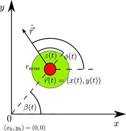
Figure 1: Schematic representation of coordinates and angles for the active searcher (red dot) in two dimensions. The position vector is $\vec{r}(t)$ with orientation $\beta(t)$, the velocity is $\vec{v}(t)=\dot{\vec{r}}(t)$. Its direction is the heading $\phi(t)$ and the angle $z(t)=\phi-\beta$ indicates the difference between the velocity and position vectors. The home is located at the origin and the green area stands for the interaction zone of the considered particle with surrounding particles.

The main ingredient of the kinematics of the searcher is the dynamics of the heading direction standing for the decision making step of the searcher to choose a new direction. In Noetel et al. (2018a, b), we assumed

$$\dot{\phi}=\kappa\sin(\phi-\beta)+\frac{\sigma}{v_{0}}\xi(t).$$ (2)

Therein, $\beta(t)\in[0,2\pi)$ is the direction of the position vector in polar coordinates $\vec{r}(t)=r(t)\{\cos(\beta(t)),\sin(\beta(t))\}$ with $r(t)$ being the distance to the home. With respect to the Cartesian coordinates the angle is linked as

$$\beta(t)=\arctan{\frac{y(t)}{x(t)}}\,.$$ (3)

The first item of the r.h.s. of the heading dynamics (2) defines a search and return mechanism. If the searcher moves outwardly, the directions of the position and the velocity vectors differ less than $|\phi-\beta|\leq\pi/2$. The heading dynamics predicts a repulsion of the heading direction from the position vector. It describes the search phase of the particle and searchers look around. Alternatively, returning to the home the two angles behave as $|\phi-\beta|\geq\pi/2$. The heading dynamics (2) leads to an anti-alignment of the heading vector with the position vector. As a result, the searcher will return to its home.

In the last term of the heading dynamics, $\xi(t)$ stands for a source of white noise with strength $\sigma$. It grants the prediction of the new direction with an uncertainty at time $t$ and might be originated by a limited knowledge of the searcher concerning the precise relations between the two angles $\beta$ and $\phi$. In the previous work we took $\alpha$-stable Levý noise modeling large rapid changes in the orientation of the velocity vector as reported for the fruit fly Kim and Dickinson (2017). In the current study we fix $\alpha=2$ which makes $\xi(t)$ to Gaussian white noise changing the heading more smoothly in a diffusive manner.

Our proposed model is strictly phenomenological. It means that we obtain the trajectories without having a neurophysiological manifestation and relations to external or internal cues. Hence, our model does not answer the questions regarding the reasons for the decisions made during the search. This decision finding (2) and the path integration (1) is formulated as a stochastic dynamics which is a kind of instantaneous dead reckoning or vector handling based on an interaction between two directions. Knowing the current orientations of the position $\beta(t)$ and heading $\phi(t)$ vectors, the future motion is defined by calculating the new heading $\phi(t+\delta t)$. How the two directions have been recovered at the given time $t$ remains open in the model. Whether this information is achieved through a earlier training, orientation flights or by internal counting processes is not answered. More detailed discussions on possible storage of spatial information and consequences for the kinematics of the searcher, the role of external cues, rewarding and different food sources is part of a larger literature Wehner and Srinivasan (1981); Russel and Norvig (2010); Forucassie and Traniello (1994); Freska and Mark (1999); Vickerstaff and Cheung (2010); Collett et al. (2013).

Otherwise, small variations of the basic dynamics (1) and (2) might model more complex behavior such as is documented in the large biological literature. The enlargement of the excursions in case of an unsuccessful search Wehner and Srinivasan (1981); Hoffmann (1983) might be modeled by weakly lowering the coupling to the home, by decreasing slowly $\kappa$ as time elapses. In contrast, a straight trajectory directly to the nest Wehner et al. (2002); Collett (2010) could be caused by a sudden switch to high values of $\kappa$. Similar modifications would allow to describe the change from an Archimedian search to the random loop. Narrow hairpin-like shaped excursions as observed for foraging search of honeybees and bumblebees Capaldi et al. (2000); Osborne et al. (2013) could be reflected by considering $\kappa$ dependent on the distance and an increase of the velocity. More difficult is the modeling of shifts of position of the searcher creating multiple fictive homes Wehner et al. (2002); Reynolds et al. (2007a) as well as a scale free flights of bees Reynolds et al. (2007b)Reynolds et al. (2007a); Lenz et al. (2013). Such detailed biological analysis of our search and return model might be the contents of a future work in a biological journal.

II.2 Resume of dynamical properties of the model

The analytical tractability of the model becomes visible if transforming to a polar presentation. Let $r(t)=\sqrt{x^{2}(t)+y^{2}(t)}$ be the distance from the origin being the localization of the home. Further on, we introduce the difference between the two directions of the position and heading vector as $z(t)=\phi(t)-\beta(t)$. The third variable is the direction $\beta(t)$ as in Eq. (3). For these new variables the equations of motion read

$$\dot{r}\,=\,v_{0}\cos(z)\,,$$

$$\dot{z}\,=\,\left(\kappa-\frac{v_{0}}{r}\right)\sin(z)\,+\,\frac{\sigma}{v_{0}}\,\xi(t)\,,$$

$$\dot{\beta}\,=\,\frac{v_{0}}{r}\sin(z)\,.$$ (4)

It is immediately seen that the $\beta(t)$ variable separates from the two others. The last equation in (4) can be integrated after having defined the couple $r(t)$ and $z(t)$.

Remarkably, the two equations for $r,z$ define without noise $\sigma=0$ a deterministic oscillatory motion in the $(r,z)$ space. Stationary fixed points of the dynamics are saddles or centers as it was reported in Noetel et al. (2018a). Trajectories perform an oscillatory loops with alternating search and return epochs. In Fig. 2 we present deterministic and stochastic trajectories as computed from Eqs.(1) and (2). The deterministic dynamics in the $(x,y)$ space creates trajectories similar to a rosette with leaves, called also random loops. The searchers return periodically to the nest. The leaves are located around the center with a fixed precession of the perihelion. Such trajectories reflect the stereotypical behavior of central place foragers, which start at the home and then move in loops from and back to the home. In Noetel et al. (2018a) we have calculated the period as well as the precession. We mention, that a similar model was introduced by Waldner and MerkleWaldner and Merkle (2018) who computed similar trajectories.

With noise the leaves become random loops. The stochastic sample path also returns permanently to the vicinity of the home in finite times. Inspection of the autocorrelation function of the distance exhibits a behavior of a damped oscillation with characteristic time $\tau_{\phi}$ from (7). Such random loops have been reported for the fruit fly Kim and Dickinson (2017) and the dessert ants Wehner and Srinivasan (1981) and isopods Hoffmann (1983). Also it was reported, that foraging honeybees Capaldi et al. (2000); Collett (2000) and bumblebees Osborne et al. (2013); Makinson et al. (2019) move along random loops.

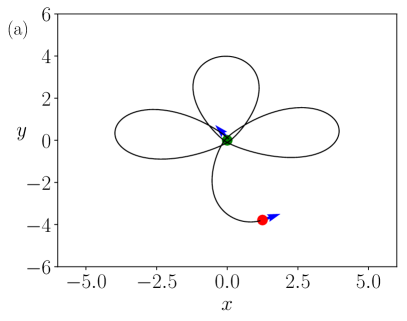
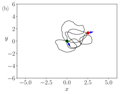
Figure 2: Sample paths of active searchers originated by Eqs.(1) and (2). (a): The deterministic case without noise $\sigma^{2}=0$. The dynamics exhibits trajectories which periodically return to the home. The shape is similar to a rosette. (b): The stochastic dynamics with Gaussian noise and $\sigma^{2}=0.1$ creates random loops around the home. Sample paths also return after finite times to the home. Parameters: $v_{0}=1$, $\kappa=1$.

Without noise the dynamics is conservative, meaning there exist an integral of motion $X$ which ins constant along the deterministic trajectories $r(t),z(t)$ with initial states $r_{0}$ and $z_{0}$. It reads

$$X(r,z)\,=\,v_{0}\sin(z)\exp\left(-\frac{\kappa}{v_{0}}r\right)\,=\,X(r_{0},z_{0})\,.$$ (5)

Since the sign of the integral $X$ is also conserved, there is no trajectory which might cross the straight lines $z=0$ or $z=\pm\pi$ in the $r,z$-space. This means that the deterministic angular momentum

$$L(r,z)\,=\,r^{2}\,\dot{\beta}=v_{0}\,r\,\sin(z)\,=\,v_{0}\,\exp\left(\frac{\kappa}{v_{0}}r\right)X(r,z),$$ (6)

along a trajectory never changes its sign. In the deterministic model a single particle either moves in a clockwise ($z>0$) or a counterclockwise $(z<0)$ fashion around the home in the Cartesian coordinate system. This behavior of single searchers is in agreement with the observations for the Daphnia Magna Ordemann et al. (2003a); Erdmann et al. (2004); Mach and Schweitzer (2007). Attracted by the light the singular Daphnia moves persistently a certain number of orbits clockwise or anti-clockwise before random influences induce a switch of the rotation sense.

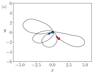
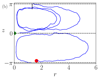
Figure 3: Sample trajectories with small noise $\sigma^{2}=0.01$. (a): Trajectory in the $(x,y)$ plane. Green dot marks the home. The particle starts close to the origin (green dot). (b): The corresponding motion in the $(r,z)$ plane. The crossing of the $z=\pm\pi$ line (indicated by the arrow) changes the sign of the angular momentum. It is caused by the action of the noise in the $z$ dynamics. Other Parameters: $v_{0}=1$, $\kappa=1$.

The existence of the noise in the model makes the full dynamics (1) and (2) irreversible. There exist a relaxation time

$$\tau_{\phi}\,=\,\left(\frac{v_{0}}{\sigma}\right)^{2}\,.$$ (7)

After $\tau_{\phi}$ all angular dynamics becomes uniform and the integral of motion is damped out. At this time scale the noise also changes the directions of rotation. This behavior is illustrated in Fig. 3 wherein we show a sample trajectory in the $(x,y)$ plane as well as in the $r,z$ one. The particle starts at the home, marked as green dot at $(x,y)=(0,0)$. A time frame of $\Delta t=30$ is shown. The trajectory is under the influence of rather continuous random disturbances which is the Gaussian case. We see that the noise creates transitions between the two half-planes in the $(r,z)$ dynamics. At values $z=0$ and $z=\pm\pi$ the deterministic part in the $z$-dynamics (4) vanishes. However, the noise can cause transitions to $z$ values with different sign corresponding to a change of the rotation mode.

As follows from Eq. (6), the angular momentum is linked directly to the integral of motion $X$. With noise this integral becomes stochastic, i.e. $X_{\xi}(t)$ and the angular momentum $L_{\xi}(t)$, as well. In Noetel et al. (2018a) we showed that in case with noise the mean value of the integral $\left\langle X_{\xi}(t)\right\rangle_{X_{0}}$ conditioned to a certain initial condition $X_{0}$ decays after the time $\tau_{\phi}$. Consequently, we might conclude that the average angular momentum will vanish as well which reflects the permanent switches of the sign of $L_{\xi}(t)$.

With noise in the angular dynamics the spatial dynamics of a single searcher becomes stationary. Initial conditions $x_{0},y_{0},\phi_{0}$ are lost and the corresponding pdf $P(x,y,\phi|x_{0},y_{0},\phi_{0},t)$ approaches for $t\to\infty$ a stationary shape $P(x,y,\phi)$ being the unique asymptotic attractor of the stochastic dynamics. Since after $\tau_{\phi}$ the angles $\phi$ and $\beta$ are equi-distributed in $[0,2\pi]$, the further evolution of the system takes place in space. This overdamped evolution can be characterized by the time at which the particle spreads by diffusion over the characteristic length $r_{c}=v_{0}/\kappa$ of this problem, i.e.

$$\tau_{r}\,=\,\frac{\sigma^{2}}{v_{0}^{2}\kappa^{2}}\,.$$ (8)

Therein we have used as diffusion coefficient $D_{\text{eff}}=v_{0}^{2}\tau_{\phi}/2$ known for an active micro-swimmer with constant speed (Mikhailov and Meinköhn, 1997; Nötel et al., 2017). In case of coupling, this diffusion coefficient changes as can seen below (see IV.5).

Both time scales (7) and (8) are determined by the value of the noise intensity but scale differently with $\sigma^{2}$. This different scaling causes an optimal noise for the mean time which is needed to find new food source in the neighborhood of the home as was reported earlier Noetel et al. (2018a).

In Noetel et al. (2018a) we also derived the Smoluchowski-equation for the marginal spatial density $\rho(x,y,t)$. Its stationary solution was found to be a exponential function

$$\rho(x,y)=\left(\frac{\kappa}{v_{0}}\right)^{2}\exp\left(-\frac{\kappa}{v_{0}}\,\sqrt{x^{2}+y^{2}}\right)$$ (9)

This marginal density agrees pretty well with experimental data from the fruit fly Kim and Dickinson (2017). Surprisingly, the marginal spatial density function to find a particle at a specific point $(x,y)$ is independent of the noise strength $\sigma$.

III Ensembles of coupled active searchers

III.1 The model of $N$ active searchers with alignment

The interacting $N$ searchers will move in two dimensions with constant speed $v_{0}$. Their common home is situated at $(x_{h},y_{h})=(0,0)$. The position vectors are given by $\vec{r}_{i}(t)=(x_{i}(t),y_{i}(t)),\,i=1,2,\ldots,N$. The direction of motion, the heading direction, is given by the angle $\phi_{i}(t)$. A schematic representation of the coordinates of a single particle is shown in Fig.1.

The equations of motion for the position are:

$$\dot{x}_{i} =v_{0}\cos(\phi_{i}(t))\,$$

$$\dot{y}_{i} =v_{0}\sin(\phi_{i}(t))\,.$$ (10)

The local search and the alignment dynamics happen in the time evolution of the heading direction:

$$\dot{\phi}_{i}=-\kappa\sin(\beta_{i}-\phi_{i})+\frac{\mu}{N_{i}}\sum_{j\in\Omega_{i}}\sin(\phi_{j}-\phi_{i})+\frac{\sigma}{v_{0}}\xi_{i}(t)\,.$$ (11)

The first term on the right hand side causes local search Noetel et al. (2018a, b) as explained above. There $\kappa$ is the common coupling strength towards the home and the $\beta_{i}(t)=\arctan(y_{i}/x_{i})$ stands again for the position angle.

The second term on the right hand side is the new alignment interaction between neighboring searchers. For simplicity, we assume a Kuramoto-like or Vicsek-like interaction of the heading directions of the searchers Kuramoto (1984); Vicsek et al. (1995); Romanczuk et al. (2012). With the assumed constant speed, it coincides with the arrayal force defined in Okubo and Levin (2002). The sum is taken over $\Omega_{i}$ which lists the current numbers $j$ of particles inside the sensing radius of particle $i$, i.e. with distances $r_{ij}=\sqrt{(x_{i}-x_{j})^{2}+(y_{i}-y_{j})^{2}}$ that obey $r_{ij}\leqslant r_{\text{sens}}$. The $N_{i}$ is the overall number of particles inside the sensing radius, respectively, the number of items in the list $\Omega_{i}$.

The coupling strength for the alignment is given by $\mu>0$. We divide the coupling strength $\mu$ by the number of neighbors to restrict the influence of the alignment on the overall motion. The searcher balances now the wish of coupling towards the home and alignment with its neighbor. The particles maintain in average a non vanishing distance as noise is present in the model and tends to uniform the particles, although we do not consider explicitly repulsion between particles. As already noticed, the couplings strength $\mu$ should be moderate to avoid density instabilities that might break the circular symmetry. In particular, we consider always $\mu\leqslant\kappa$.

The third term on the right hand side represents Gaussian white noise with $\langle\xi_{i}(t)\rangle=0$ and $\langle\xi_{i}(t)\xi_{j}(t^{\prime})\rangle=2\delta_{ij}\delta(t-t^{\prime})$. It describes an uncertainty in the decision of the new direction. Noise sources of different particles are considered to be uncorrelated. The parameter $\sigma$ denotes an unique noise strength for all particles.

III.2 Numerical results of aligning active searchers

Fig.4 shows a snapshot of the positions and headings of $N=1000$ searchers. The trajectory of an individual searcher is shown in the insets of the graph. For picture (a) a coupling strength of $\mu=0.1$ and for (b) a coupling of $\mu=0.7$ was chosen.

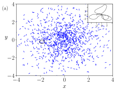
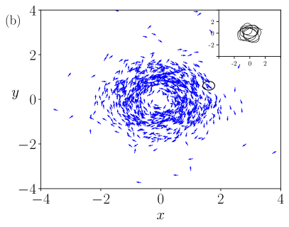
Figure 4: (a): Snapshot of searchers with small alignment $\mu=0.1$ according to Eqs. (10) and (11). Searchers will follow their individual strategies and no cooperative behavior is observed. (b): Snapshot of searchers with alignment $\mu=0.7$. For sufficient alignment strength the searchers form a rotating circle around the home. Rotations might be clockwise or anticlockwise in dependence on initial values. Black lines in the insets indicate one individual trajectory over a longer period of time. The random loops in the undercritical regime turn into circular motion for overcritical coupling $\mu$. Circles indicate the size of the sensing radius. Parameters: $N=1000$, $v_{0}=1$, $\kappa=1$, $r_{\text{sens}}=0.2$, $\sigma^{2}=0.1$.

While the searchers in (a) perform individual search motion in case of weak $\mu$, they collectively rotate around their common home or target in (b). Therefore, we expect to find a transition at a critical value of the coupling strength $\mu_{\text{crit}}$ between individual motion $\mu<\mu_{\text{crit}}$ and collective motion $\mu>\mu_{\text{crit}}$. We also note that the foragers in (a) are more spread out over the space than the foragers in (b). The insets show typical individual trajectories. The individual trajectories change from central place foraging motion (a) to circular motion (b).

We will investigate how the asymptotic marginal densities of the distance from the home as well as the marginal density of the difference between the heading and the direction of the position vector change if varying the coupling strength $\mu$. A critical behavior is predicted for the mean orbital velocity of the active local searchers in dependence on the relation between $\mu$ to the ratio between the value $v_{0}$ and the noise intensity $\sigma$. In consequence, also the variances of the radial and orbital velocities will exhibit different behavior for small and large coupling

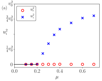
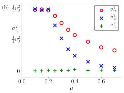
Figure 5: (a): Squared average radial and orbital velocities from simulations as symbols. Beyond the critical coupling strength $\mu_{\text{crit}}\approx 0.2$ a cooperative rotating of the searchers around the home is instigated which gains all energy for strong coupling. (b): The covariance and the variance of the orbital and radial velocity fluctuations as function of the coupling strength $\mu$. The covariance vanishes at arbitrary coupling. In the cooperative regime both variances decay with different strength and disappear for large coupling strength. Parameters: $N=1000$, $v_{0}=1$, $\kappa=1$, $\sigma^{2}=0.1$, $r_{\text{sens}}=0.2$.

In Fig.5 we present results in the asymptotic long time state which quantify the two different regimes. We measured during the simulations of $N=1000$ particles the mean radial $u_{r}$ and orbital $u_{z}$ velocities and the variances and the covariance $\sigma^{2}_{rr},\sigma^{2}_{zz}$, and $\sigma^{2}_{rz}$ of their fluctuations. We point out that all presented values in pictures (a) and (b) are independent on space. These velocity characteristics loose possible initial dependencies on coordinates in the asymptotic limit. They become homogeneous in space at least at the places where a sufficiently large number of particles is present during the measurements. On the left hand side the stationary mean velocities are presented as functions of the coupling strength $\mu$. The asymptotic radial velocity vanishes always independently from $\mu$. In difference, the squared angular velocity exhibits a soft transition at $\mu_{\text{crit}}\approx 0.2$. For lower coupling strength it vanishes as well, for $\mu$-values larger the critical one an orbital motion is created. The orbital squared velocity grows with stronger coupling and saturates at $v_{0}^{2}$ for infinitely large coupling where all energy is in the circular drift. The direction (clockwise or anti-clockwise) of the rotation around the home depends on initial values and with noise even changes in the direction of the rotations are possible.

Fig. 5(b) shows asymptotic of the second central moments. One sees that the covariance $\sigma_{rz}^{2}$ of radial and orbital velocity fluctuations disappears, thoroughly. For under-critical coupling strength the variances $\sigma_{rr}^{2}$ and $\sigma_{zz}^{2}$ share the same value which is half of the possible kinetic energy. In case of an over-critical coupling strength both variances shrink and vanish as $\mu\to\infty$. The decay of the orbital velocity fluctuations is stronger than the radial fluctuations decrease with growing $\mu$.

The occurrence of ordered circular motion is accompanied by a change in the distribution of the $z$ angle. The latter is uniform for an under-critical coupling strength. The distributions of the position angle $\beta$ and of the heading $\phi$ remain uniform also with over-critical couplings strength. The marginal pdf $\rho_{z}(z)$ of their difference $z$ exhibits a maximum at a fixed position if the coupling becomes over-critical. It is presented in Fig.6 where the marginal $z$-density as obtained from numeric simulations is shown for various values of $\mu$. The particular situation with a peak at $z=-\pi/2$ corresponds to the clockwise rotation of the aligning units around the home. Alternatively, the anticlockwise motion might collect maximal probability above $z=\pi/2$. Symmetry in the $2\pi$ periodic $z$ space is established with respect to $\pm\pi/2$, meaning $\rho_{z}(\pm\pi/2+z^{\prime})=\rho_{z}(\pm\pi/2-z^{\prime})$.

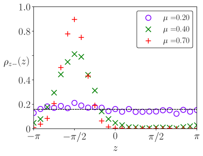
Figure 6: Simulation results for the marginal density of the angle $z$ as symbols for three different values of the coupling $\mu$. The simulation results were chosen for $u_{z}<0$, meaning clockwise rotation in the $(x,y)$ plane. For counterclockwise rotation the densities are shifted by $\pi$. All three values for the coupling are chosen $\mu>\mu_{\text{crit}}=0.2$. The dashed line corresponds to a uniform density. This density is approached for $\mu=\mu_{\text{crit}}$. Parameters: $N=1000$, $v_{0}=1$, $\kappa=1$, $\sigma^{2}=0.1$, $r_{\text{sens}}=0.2$.

For a system with a finite particle number $N$ as defined by the set of Langevin equations in our model, the asymptotic marginal $z$ pdf is always the sum of two pdf’s, one with a clockwise and the other with a anti clockwise rotations. Due to the symmetry of this bistable situation connected with possible transitions between the two directions of rotation, both pdf’s contribute equally to the steady pdf. Alternatively, in the thermodynamic limit as considered in the following analytic approach, ergodicity is broken and as final state we get one of the two possible pdf’s in dependence on the initial state. Later on in the discussion of the analytical results, we restrict the consideration to the particular type of clock wise rotations.

III.3 Polar presentation of the particle dynamics

We change to polar coordinates, i.e., to the distance $r_{i}(t)=\sqrt{x_{i}^{2}(t)+y_{i}^{2}(t)}$ and the direction $\beta_{i}(t)=\arctan(y_{i}(t)/x_{i}(t))$ of the position vector $\vec{r}_{i}(t)$ (see Fig 1). Furthermore, we introduce the angle $z_{i}(t)=\phi_{i}(t)-\beta_{i}(t)$, being the difference between the heading and the position. A value of $z=\pi/2$ indicates counterclockwise rotation, a value of $z=-\pi/2$ clockwise rotation. Alternatively, values around $0$ and $\pi$ stand for motion pointing outwards, respectively, towards the home. Simulations in Fig. 4(b) show a clockwise rotation of the aligned collective motion, hence maximal probability in the $z$-distribution is expected for values around $z\approx-\pi/2$.

We derive for the radial velocity:

$$\dot{r}_{i}=v_{0}\cos(z_{i})\,,$$ (12)

and for the angular velocity:

$$\dot{\beta}_{i}=\frac{v_{0}}{r_{i}}\sin(z_{i})\,.$$ (13)

The dynamics for the angle $z$ becomes:

$$\dot{z}_{i}=-\left(\frac{1}{r}-\frac{1}{r_{c}}\right)v_{0}\sin(z_{i})+\frac{\mu}{N_{i}}\sum_{j\in\Omega_{i}}\sin(z_{j}-z_{i}+\beta_{j}-\beta_{i})+\frac{\sigma}{v_{0}}\xi_{i}(t)\,,$$ (14)

where again $r_{c}=v_{0}/\kappa$ and $\Omega_{i}$ contains the indices of the $N_{i}$ particles within the sensing radius of the particle $i$.

For the third equation (14), we assume that the position angles $\beta_{i}\approx\beta_{j}$ cancel each other. The $z$ dynamics becomes:

$$\dot{z}_{i}=-\left(\frac{1}{r}-\frac{1}{r_{c}}\right)v_{0}\sin(z_{i})+\frac{\mu}{N_{i}}\sum_{j\in\Omega_{i}}\sin(z_{j}-z_{i})+\frac{\sigma}{v_{0}}\xi_{i}(t)\,.$$ (15)

This approximation is valid if having a sufficient small sensing radius $r_{\text{sens}}\ll r_{c}=v_{0}/\kappa$. Therein $r_{c}$ appears as the distance where searchers reside with maximal probability which will be shown, later on. The approximation fails obviously for small distances from the home. Hence, the typical length scales of (15) should be much larger than the interaction radius, i.e. $r\gg r_{\text{sens}}$.

And thus, the searchers are described by the actual values of the set $r_{i}(t),\beta_{i}(t)$ and $z_{i}(t)$. For a single independent searcher $(\mu=0)$ the $(r(t),z(t))$ dynamics separates from the $\beta(t)$ dynamics Noetel et al. (2018a). With alignment present this is not the case as the position angle enters the $z_{i}$ dynamics through the neighborhood $\Omega_{i}$. Nevertheless, as will be discussed now, at larger time scales $t\gg\tau_{\phi}$ the $\beta_{i}$ become uniform distributed as well as the heading directions $\phi_{i}$ do. Only their binary relation expressed by $z_{i}(t)$ will matter for the behavior.

IV Probability density function and transport equations

IV.1 The nonlinear Fokker-Planck equation with effective aligning force

We consider the many particle pdf $P_{N}(r_{1},z_{1},\beta_{1},\ldots,r_{N},z_{N},\beta_{N},t)$ in polar presentation. We consider the pdf to be well approximated by the product of the one particle PDF $P(r,z,\beta,t)$ having in mind the limit of infinite particle numbers and assuming the validity of a mean field approximation. In consequence, we formulate the alignment force $f_{al}(r,\beta,z,t)$ which a particle experiences at position $r,\beta$ from a second particle with coordinates $r^{\prime},\beta^{\prime}$ inside the sensing radius of the first one $\Omega(r,\beta)$ as:

$$f_{al}(r,z,\beta,t)\,=\,\frac{\mu}{N_{\text{sens}}(r,\beta,t)}\,N\,\int_{(r^{\prime},\beta^{\prime})\in\Omega(r,\beta)}{\rm{d}}r^{\prime}{\rm{d}}\beta^{\prime}\int_{-\pi}^{\pi}{\rm{d}}z^{\prime}\,\sin(z^{\prime}-z)\,P(r^{\prime},\beta^{\prime},z^{\prime},t)\,.$$

(16)

The particle density in the sensing region reads accordingly

$$N_{\text{sens}}(r,\beta,t)\,=\,N\,\int_{(r^{\prime},\beta^{\prime})\in\Omega(r,\beta)}{\rm{d}}r^{\prime}{\rm{d}}\beta^{\prime}\int_{-\pi}^{\pi}{\rm{d}}z^{\prime}\,P(r^{\prime},\beta^{\prime},z^{\prime},t)\,.$$ (17)

For the further evaluation of (16), we introduce the marginal spatial pdf $\rho(r,\beta,t)$ and the mean velocities $u_{r}(r,\beta,t)$, $u_{z}(r,\beta,t)$ in dependence of the polar coordinates $r,\beta$ as

$$\rho(r,\beta,t) =\int_{-\pi}^{\pi}{\rm{d}}zP(r,\beta,z,t)\,,$$ (18)

$$u_{r}(r,\beta,t)\rho(r,\beta,t) =v_{0}\int_{-\pi}^{\pi}{\rm{d}}z\cos(z)P(r,\beta,z,t)\,,$$ (19)

$$u_{z}(r,\beta,t)\rho(r,\beta,t) =v_{0}\int_{-\pi}^{\pi}{\rm{d}}z\sin(z)P(r,\beta,z,t)\,.$$ (20)

Introducing (18)-(20) into the interaction term (16) and performing the $z^{\prime}$ integration, leads to:

$$f_{al}(r,\beta,t)\,=\,$$ (21)

$$\frac{\mu}{N_{\text{sens}}(r,\beta,t)}N\int_{(r^{\prime}\beta^{\prime})\in\Omega(r,\beta)}{\rm{d}}r^{\prime}{\rm{d}}\beta^{\prime}\,\left(u_{z}(r^{\prime},\beta^{\prime},t)\cos(z)-u_{r}(r^{\prime},\beta^{\prime},t)\sin(z)\right)\,\rho(r^{\prime},\beta^{\prime},t)\,.$$

With the above assumptions about a small sensing radius $r_{\text{sens}}$ and that distances are with high probability around $r\approx r_{c}$ one can simplify the expressions (16) and (17). We equalize positions and directions $r\approx r^{\prime}$ and $\beta\approx\beta^{\prime}$ inside the integral. It means that for sufficient small sensing radius the average velocities as well as the marginal density are constant inside this radius. It results in $u_{r}(r^{\prime},\beta^{\prime},t)\approx u_{r}(r,\beta,t)$ and $u_{z}(r^{\prime},\beta^{\prime},t)\approx u_{z}(r,\beta,t)$. The same approximation is done in the expression for the $N_{\text{sens}}(r,\beta,t)$ in Eq. (17). The latter drops together with the density $N\,\rho(r^{\prime},\beta^{\prime},t)\,\pi r_{\text{sens}}^{2}\approx N_{\text{sens}}(r,\beta,t)$ in Eq.(16). In consequence, it follows for the effective aligning force (16):

$$f_{al}\,\approx\,\mu\left(u_{z}(r,\beta,t)\cos(z)-u_{r}(r,\beta,t)\sin(z)\right)\,.$$ (22)

Note, that $u_{z}$ is defined as an orbital velocity being orthogonal to $u_{r}$. It is neither an average angular velocity for the position angle $\beta$ nor is it an average angular velocity derived from the $z(t)$ dynamics given by Eq. (14).

Fig. 4(b) shows the particles rotating homogeneously around the home. Also the disordered motion on the l.h.s. possesses rotational symmetry. Both snapshots have equilibrated around the center which is true as $t\geqslant\tau_{\phi}$. The noise has created this rotationally symmetric shape of the heading directions $\phi$ as well as the directions of the position vector $\beta$. Hence, in the following we will assume rotational symmetry for the $\beta$ and $\phi$ dynamics. We will not üpay attention to the relaxation of angular inhomogeneities of these two variables being more interested in the properties of the asymptotic state as functions of $r$.

In consequence, the marginal density (24) becomes $\rho(r,\beta,t)\approx\rho(r,t)$, and the mean velocities (19) and (20) are approximated as $u_{r}(r,\beta,t)\approx u_{r}(r,t)$ and $u_{z}(r,\beta,t)\approx u_{z}(r,t)$.

As we approximated the alignment term (22) independent of the position angle the $(r,z)$ dynamics separates from the angular $\beta$ dynamics. Also the one particle pdf looses the $\beta$ dependence. Hence the Fokker-Planck equation (FPE) is given by:

$$\frac{\partial}{\partial t}P =-v_{0}\frac{\partial}{\partial r}\cos(z)P+$$

$$+v_{0}\frac{\partial}{\partial z}\left(\left(\frac{1}{r}-\frac{1}{r_{c}}+\frac{\mu}{v_{0}^{2}}u_{r}\right)\sin(z)-\frac{\mu}{v_{0}^{2}}u_{z}\cos(z)\right)P+\left(\frac{\sigma}{v_{0}}\right)^{2}\frac{\partial^{2}}{\partial z^{2}}P\,,$$

and $P$ is the transition pdf $P=P(r,z,t|r_{0},z_{0},t_{0})$ describing the reduced $(r,z)$ dynamics. This FPE is valid for large particle numbers $N\to\infty$, vanishing sensing radius $r_{\text{sens}}\ll r_{c}$ and at time scales $t\geqslant\tau_{\phi}$. The equation is nonlinear in $P$ since the $u_{r}$ and $u_{z}$ are functions of the pdf.

IV.2 Transport equations

In order to find approximate solutions, we derive transport equations for the first three moments (18), (19) and (20) being now independent of $\beta$. By respective standard multiplication of the FPE and integration over $z$ we obtain relations between the reduced moments of trigonometric functions depending on space and time. The marginal density of the distance obeys the continuity equation

$$\frac{\partial}{\partial t}\rho=-\frac{\partial}{\partial r}\rho u_{r}\,.$$ (24)

The equations of the first moments read for the mean radial velocity

$$\frac{\partial}{\partial t}u_{r}\rho=$$ (25)

$$-\frac{\partial}{\partial r}\rho\left(u_{r}^{2}+\sigma_{rr}^{2}\right)+\left(\frac{1}{r}-\frac{1}{r_{c}}\right)\rho\left(u_{z}^{2}+\sigma_{zz}^{2}\right)-\frac{\mu}{v_{0}^{2}}\rho u_{z}\sigma_{rz}+\left(\frac{\mu}{v_{0}^{2}}\sigma_{zz}^{2}-\left(\frac{\sigma}{v_{0}}\right)^{2}\right)\rho u_{r}\,,$$

and for the mean orbital velocity

$$\frac{\partial}{\partial t}u_{z}\rho=$$ (26)

$$-\frac{\partial}{\partial r}\rho\left(u_{r}u_{z}+\sigma_{rz}^{2}\right)-\left(\frac{1}{r}-\frac{1}{r_{c}}\right)\rho\left(u_{r}u_{z}+\sigma_{rz}^{2}\right)-\frac{\mu}{v_{0}^{2}}\rho u_{r}\sigma_{rz}^{2}+\left(\frac{\mu}{v_{0}^{2}}\sigma_{rr}^{2}-\left(\frac{\sigma}{v_{0}}\right)^{2}\right)\rho u_{z}\,.$$

Therein, we have introduced the variances as

$$\sigma^{2}_{rr}(r,t)\rho(r,t) =\int_{-\pi}^{\pi}{\rm{d}}z\,v_{0}\cos^{2}(z)\,P(r,z,t)\,-\,u_{r}^{2}\,\rho,$$

$$\sigma^{2}_{zz}(r,t)\rho(r,t) =\int_{-\pi}^{\pi}{\rm{d}}z\,v_{0}\sin^{2}(z)\,P(r,z,t)\,-\,u_{z}^{2}\,\rho\,.$$ (27)

Note that due to the constant speed of the particles the variances and mean velocities are not independent

$$\sigma^{2}_{rr}+u^{2}_{r}+\sigma^{2}_{zz}+u^{2}_{z}=v_{0}^{2}\,.$$ (28)

One of these values might be expressed by the three other moments.

We have also introduced the covariance as

$$\sigma^{2}_{rz}(r,t)\rho(r,t) =\int_{-\pi}^{\pi}{\rm{d}}z\,v_{0}^{2}\cos(z)\,\sin(z)\,P(r,z,t)\,-\,u_{r}u_{z}\rho\,.$$ (29)

In our theoretical consideration we will assume that the two velocity deviations from their mean $\delta u_{r}=v_{0}\cos(z)-u_{r}$ and $\delta u_{z}=v_{0}\sin(z)-u_{z}$ are not correlated. It was shown numerically for the asymptotic stationary limit as presented above (see Fig.5). We simplify our model here and will neglect the correlation by putting $\sigma_{rz}(r,t)=0$, further on.

We derive for the second moments (see Eqs.(27)):

$$\frac{\partial\rho\left(u_{r}^{2}+\sigma_{rr}^{2}\right)}{\partial t} \,=\,-\frac{\partial}{\partial r}\langle v_{0}^{3}\cos^{3}(z)\rangle\,+\,2\left(\frac{1}{r}-\frac{1}{r_{c}}\right)\langle v_{0}^{3}\cos(z)\sin^{2}(z)\rangle$$

$$+\frac{2\mu}{v_{0}^{2}}\left(u_{r}\langle v_{0}^{3}\cos(z)\sin^{2}(z)\rangle-u_{z}\langle v_{0}^{3}\cos^{2}(z)\sin(z)\rangle\right)+\frac{4\sigma^{2}}{v_{0}^{2}}\rho\left(\frac{v_{0}^{2}}{2}-(u_{r}^{2}+\sigma_{rr}^{2})\right),$$

and

$$\frac{\partial\rho\left(u_{z}^{2}+\sigma_{zz}^{2}\right)}{\partial t} \,=\,-\frac{\partial}{\partial r}\langle v_{0}^{3}\cos(z)\sin^{2}(z)\rangle\,-\,2\left(\frac{1}{r}-\frac{1}{r_{c}}\right)\langle v_{0}^{3}\cos(z)\sin^{2}(z)\rangle$$

$$-\frac{2\mu}{v_{0}^{2}}\left(u_{r}\langle v_{0}^{3}\cos(z)\sin^{2}(z)\rangle-u_{z}\langle v_{0}^{3}\cos^{2}(z)\sin(z)\rangle\right)+\frac{4\sigma^{2}}{v_{0}^{2}}\rho\left(\frac{v_{0}^{2}}{2}-\left(u_{z}^{2}+\sigma_{zz}^{2}\right)\right)\,,$$

where we made use already of the assumed simplification.

In subsection IV.4 we will decouple higher moments in equations for second velocity moments. One usual way would be a Gaussian approximation of this higher moments. This case and its results are presented in the Appendix B. Here in the next subsection IV.3 we will derive an expression for the marginal density $\rho_{z}(z)$ of the angular variable $z$ outgoing from the nonlinear FPE (IV.1). It will be a von Mises distribution. The resulting decoupling scenario yields better agreement between the transport theory and the numeric findings.

IV.3 The marginal $z$-density as von Mises distribution

The marginal density $\rho_{z}(z.t)$ of the angular variable $z$ is defined by the integral

$$\rho_{z}(z,t)=\int_{0}^{\infty}{\rm{d}}rP(r,z,t)\,.$$ (32)

Likewise for the spatial marginal density, we derive here a dynamics for $\rho(z,t)$ starting from the FPE (IV.1) and integrating away this time the distance $r$. The corresponding FPE reads:

$$\frac{\partial}{\partial t}\rho_{z}=v_{0}\frac{\partial}{\partial z}\left(\left\langle\frac{1}{r}-\frac{1}{r_{c}}+\frac{\mu}{v_{0}^{2}}u_{r}\right\rangle_{r}\sin(z)-\frac{\mu}{v^{2}_{0}}\langle u_{z}\rangle_{r}\cos(z)\right)\rho_{z}+\left(\frac{\sigma}{v_{0}}\right)^{2}\frac{\partial^{2}}{\partial z^{2}}\rho_{z}\,.$$ (33)

In this equation we formally abbreviated $\left\langle\,.\,\right\rangle_{r}=\int{\rm d}r\,.\,P(r,t|z)$ and $P(r,t|z)$ is the conditional pdf of a distance $r$ for a fixed $z$. In simulations this dependence on $z$ appeared to be weak. In order to obey the numerically found asymptotic $z$-symmetry, the bracket in front of the $\sin(z)$ function in (33) should disappear for arbitrary $z$-values. Extrema of the density $\rho_{z}$ have been found at angles where the $\cos(z)$-function vanishes. Therefore, it holds $\langle 1/r-1/r_{c}+\mu u_{r}/v_{0}^{2}\rangle_{r}=0$. The velocity $u_{z}$ becomes asymptotically constant and homogeneous in space as well. The bracket can be dropped and we write $\langle u_{z}\rangle_{r}=u_{z}$. With these settings we can integrate the stationary FPE. The marginal angular pdf (32) yields a von Mises distribution Stratonovich (1967); Kürsten and Ihle (2017) which reads

$$\rho_{z}(z)\,=\,\frac{1}{2\pi I_{0}\left(\frac{\mu u_{z}v_{0}}{\sigma^{2}}\right)}\exp\left(\frac{\mu u_{z}}{\sigma^{2}}v_{0}\sin(z)\right)\,.$$ (34)

Therein the $I_{n}$ stands for the modified Bessel function of the first kind.

In dependence on the sign of $u_{z}$ the von Mises distribution peaks above one of the values $z=\pm\pi/2$ and has the minimum at $z=\mp\pi/2$. Since we deal with a nonlinear FPE, ergodicity is broken in the over-critical solution and the asymptotic solution depends on initial states. With under-critical coupling strength no mean orbital drift exists $u_{z}=0$ and the von Mises distribution collapses into the uniform distribution.

The von Mises distribution allows a self-consistent definition of the stationary mean orbital velocity $u_{z}$. The latter is given as the solution of the expression:

$$u_{z}=\frac{1}{2\pi I_{0}\left(\frac{\mu u_{z}v_{0}}{\sigma^{2}}\right)}\int_{-\pi}^{\pi}{\rm{d}}z\,\,v_{0}\sin(z)\,\exp\left(\frac{\mu u_{z}}{\sigma^{2}}v_{0}\sin(z)\right)\,=\,v_{0}\frac{I_{1}\left(\frac{\mu u_{z}v_{0}}{\sigma^{2}}\right)}{I_{0}\left(\frac{\mu u_{z}v_{0}}{\sigma^{2}}\right)}\,.$$ (35)

Such self-consistent relations are well known from many disciplines in physics. Exemplarily we remind on atom physics (Slater, 1959), on plasma physics (Balescu, 1960), chemical physics (Mukamel et al., 1978), the theory of equilibrium(Stanley, 1971; Kadanoff, 2009) and nonequilibrium (den Broeck et al., 1997; Sagués et al., 2007) phase transitions, and on synchronization phenomena of phase oscillators(Kuramoto, 1984; Strogatz, 2000). The usual way of finding the solution is the geometric construction of the l.h.s and the r.h.s. Their intersection(s) yield the solution of (35). It is known that this solution $u_{z}$ undergoes a pitchfork bifurcation at

$$\mu_{\text{crit}}=2\sigma^{2}/v_{0}^{2}\,.$$ (36)

It is just the value of the coupling strength at which the slope of the r.h.s. of (35) taken as function of the velocity $u_{z}$ coincides with the one from the l.h.s. in the limit of vanishing velocity. For smaller coupling a single solution $u_{z}=0$ exists, only. For over-critical coupling $\mu>\mu_{\text{crit}}$ there are three intersections in (35). One of them again vanishes and appears to be unstable with respect to small perturbations. The other two are stable solutions with different sign and identical non-vanishing absolute value.

Later on, in the discussion part we present also the results obtained by means of the von Mises distribution. In the next subsection, the latter is used for decoupling the higher moments in the transport equations.

IV.4 Analysis of the stationary asymptotic state

In this section we study the stationary states as they follow from the asymptotic limit of the transport equations and use the results of the last chapter.

IV.4.1 Under-critical coupling strength

First, we take a look upon the stationary limit for the case $\mu\leqslant\mu_{\text{crit}}$. There no cooperation in the motion exists and the orbital velocity disappears $u_{z}(r)=0$. The density $\rho(r,t)\to\rho(r)$ becomes stationary as well. The radial flux $u_{r}$ disappears which is a consequence of the continuity equation (24). This disappearance can be confirmed by calculating the stationary mean flux using the von Mises distribution.

At second, with $u_{z}=0$ the orbital angle distribution $\rho_{z}(z)$ squeezes to the periodic equidistribution on $z\in[-\pi,\pi)$. It causes the disappearance of all third order moments in the balance equations. Therefore, in agreement with Eqs. (IV.2) and (IV.2) the variances share the same stationary energies with

$$\sigma^{2}_{rr}\,=\,\sigma^{2}_{zz}\,=\,\frac{v_{0}^{2}}{2}\,.$$ (37)

The equation for the orbital flux reads

$$0\,=\,\frac{\partial}{\partial t}u_{z}\,=\,\left(\frac{\mu}{2}-\left(\frac{\sigma}{v_{0}}\right)^{2}\right)\,u_{z}$$ (38)

where we have dropped the stationary density and inserted the radial variance from (37). Obviously, it possesses the solution $u_{z}=0$ which is homogeneous in space as also the variances in (37) are.

Eq. (38) also defines the border of stability of the present solution. The bracket at the r.h.s. vanishes at the critical coupling strength $\mu_{\text{crit}}$ from (36). Stability of the non-cooperative behavior is given only for under-critical values $\mu$.

The single value which depends on coordinates is the marginal density $\rho(r)$. The equation which determines its functional dependence is the stationary equation for the mean radial flux $\rho u_{r}$. It becomes with the findings from above

$$0=\frac{\partial}{\partial t}\rho u_{r}\,=\,-\,\frac{v_{0}^{2}}{2}\left(\frac{\partial}{\partial r}\rho+\left(\frac{1}{r}-\frac{1}{r_{c}}\right)\rho(r)\right)\,.$$ (39)

As solution for the weakly coupled ensemble, we obtain the same stationary marginal density as it was derived for a single independent particle Noetel et al. (2018a, b). There we have found

$$\rho(r)\,=\,\frac{r}{r^{2}_{c}}\exp\left(-\frac{r}{r_{c}}\right)\,.$$ (40)

which we obtain here for the marginal density of weakly coupled searchers. We note that all moments with three trigonometric functions disappear. Hence, with the given variances (37) and vanishing fluxes all stationary transport equations are exactly fulfilled. Also the average $\langle{1}/{r}-{1}/{r_{c}}+\mu u_{r}/v_{0}^{2}\rangle_{r}$ vanishes with (40) which we used to obtain the von Mises distribution as in (34).

IV.4.2 Over-critical coupling strength

Secondly, we formulate decoupling relations for the moments including three trigonometric functions if $\mu\geqslant\mu_{\text{crit}}$ with $u_{z}\neq 0$ in agreement with the simulations and the von Mises distribution. Here, we follow a partial integration scheme of the stationary von Mises distribution. Doing so and requiring $u_{z}\neq 0$ we obtain the identity

$$u_{z}\int_{0}^{2\pi}{\rm d}z\,f(z)v_{0}\cos(z)\rho_{z}(z)\,=\,-\,\frac{\sigma^{2}}{\mu}\,\int_{0}^{2\pi}{\rm d}z\frac{{\rm d}f(z)}{{\rm d}z}\rho_{z}(z)$$ (41)

with $\rho_{z}(z)$ from (34) and $f(z)$ as polynomial of $\cos(z)$ and $\sin(z)$ functions. Note, that at the r.h.s. the single $\cos(z)$ function has disappeared and the order of the moment is reduced.

Using (41) and properties of the trigonometric functions one easily verifies that the expressions vanish for $f(z)=\cos^{2}(z)$ and $\sin^{2}(z)$. It also vanishes for $f(z)=v_{0}$ meaning again that the stationary radial flux disappears. i.e. $u_{r}(r)=0$, and the density becomes stationary $\rho(r,t)\to\rho(r)$.

And thus, the two remaining third order moments in our theory are linked to the second order moments. It holds

$$u_{z}\langle v_{0}^{3}\sin(z)\cos^{2}(z)\rangle=\rho\frac{\sigma^{2}}{\mu}\left(u_{z}^{2}+\sigma_{zz}^{2}-u_{r}^{2}-\sigma_{rr}^{2}\right)\,,$$ (42)

$$u_{z}\langle v_{0}^{3}\sin^{3}(z)\rangle=\rho v_{0}^{2}u_{z}^{2}-\rho\frac{\sigma^{2}}{\mu}\left(u_{z}^{2}+\sigma_{zz}^{2}-u_{r}^{2}-\sigma_{rr}^{2}\right)\,.$$ (43)

Afterwards, insertion of those expressions into the r.h.s. of the balance equations for the mean radial and orbital energies (IV.2) and (IV.2), we derive exactly

$$\rho\frac{\partial}{\partial t}\sigma_{rr}^{2}\,=\,0\,,~{}~{}~{}~{}~{}~{}~{}~{}~{}\rho\frac{\partial}{\partial t}\left(u_{z}^{2}+\sigma_{zz}^{2}\right)\,=\,0\,.$$ (44)

The transport equations confirm the decoupling by means of the von Mises distribution and both radial and orbital energies become stationary.

The stationary equation for the mean orbital velocity yields the same condition as in the under-critical case

$$0=\frac{\partial}{\partial t}u_{z}\,=\,\left(\frac{\mu}{v_{0}^{2}}\sigma^{2}_{rr}-\left(\frac{\sigma}{v_{0}}\right)^{2}\right)\,u_{z}\,.$$ (45)

Again the density drops out in the stationary state and this equation possesses spatially homogeneous steady states. One solution is $u_{z}=0$ which appears to be stable for under-critical coupling $\mu\leqslant\mu_{\text{crit}}$ as discussed above. Since by assumption $u_{z}\neq 0$ we select as solution for the cooperative regime

$$\sigma^{2}_{rr}\,=\,\frac{\sigma^{2}}{\mu}\,.$$ (46)

One might add here that the same expression could be obtained by determining the stationary mean radial energy via averaging with the von Mises distribution and setting $u_{r}=0$.

The equation for mean radial velocity $u_{r}$ becomes the equation for determining the marginal density $\rho(r)$. Insertion of (46) into (25) gives

$$0=\rho\frac{\partial}{\partial t}u_{r}\,=\,-\frac{\partial}{\partial r}\frac{\sigma^{2}}{\mu}\rho+\left(\frac{1}{r}-\frac{1}{r_{c}}\right)\left(v_{0}^{2}-\frac{\sigma^{2}}{\mu}\right)\rho\,.$$ (47)

This equation can be integrated and we get the steady state of the spatial marginal density in case of $\mu\geqslant\mu_{c}$:

$$\rho(r)=C\left[r\exp\left(-\frac{\kappa}{v_{0}}r\right)\right]^{\frac{v_{0}^{2}\mu}{\sigma^{2}}-1}\,,$$ (48)

with $C$ being the normalization constant. We mention that in case of the critical coupling strength, i.e. if $\mu=\mu_{c}$ the exponent in this distribution becomes unity. Hence, the marginal density (48) at critical coupling strength coincides with the marginal density in the under-critical situation (40) reminding the soft character of the pitchfork bifurcation.

In the cooperative regime the marginal density also depends on the coupling strength and on the noise intensity. In comparison to (40) the density in (48) appears more narrow above its maximal state $r_{c}$ as can be inspected in Fig.4. That is why, the exponent is larger than unity in the over-critical situation. We also remark, that again the spatial average of $\langle 1/r-1/r_{c}+\mu u_{r}/v_{0}^{2}\rangle_{r}$ vanishes.

To close the analysis, we have to determine the mean orbital velocity and its variance. The latter can be obtained using the conservation of speed (28) as variance

$$\sigma^{2}_{zz}\,=\,v_{0}^{2}-\sigma^{2}_{rr}-u^{2}_{z}$$ (49)

and it remains to determine the stationary $u_{z}$.

We could rely here to the result of the self-consistent solution (35) using the von Mises distribution. But we will follow again the transport equations to obtain an analytic expression. For this purpose we inspect the balance for the second mixed moment $\rho u_{r}u_{z}$. In case of under-critical coupling $u_{r}=0$ and $u_{z}=0$ and both sides of the balance equation vanish. In case of an over-critical coupling the equation reads

$$\frac{\partial\rho u_{r}u_{z}}{\partial t} \,=\,-\frac{\partial}{\partial r}\langle v_{0}^{3}\cos^{2}(z)\sin(z)\rangle\,+\,2\left(\frac{1}{r}-\frac{1}{r_{c}}\right)\left(\langle v_{0}^{3}\sin^{3}(z)\rangle-\langle v_{0}^{3}\cos^{2}(z)\sin(z)\rangle\right)$$ (50)

$$+\frac{2\mu}{v_{0}^{2}}u_{r}\left(\langle v_{0}^{3}\sin^{3}(z)\rangle-\langle v_{0}^{3}\cos^{2}(z)\sin(z)\rangle\right)-\frac{4\sigma^{2}}{v_{0}^{2}}\rho u_{r}u_{z}.$$

wherein we start to decouple as we did before. We obtain ($u_{z}\neq 0$)

$$0=u_{z}\frac{\partial}{\partial t}\rho u_{r}u_{z}\,=\,-\left(v_{0}^{2}-\frac{2\sigma^{2}}{\mu}\right)\frac{\partial}{\partial r}\frac{\sigma^{2}}{\mu}\rho-\left(\frac{1}{r}+\frac{1}{r_{c}}\right)\rho\left(v_{0}^{2}u_{z}^{2}-\frac{2\sigma^{2}}{\mu}\left(v_{0}^{2}-\frac{2\sigma^{2}}{\mu}\right)\right)$$

(51)

To be in agreement with the equation for the stationary marginal density (47) we have to require that the mean orbital velocity is homogeneous in space and becomes

$$u_{z}^{2}\,=\,v_{0}^{2}-\frac{\sigma^{2}}{\mu}\left(1+\frac{2\sigma^{2}}{\mu v_{0}^{2}}\right)\,.$$ (52)

Afterwards, we can complete the set of stationary characteristics. We find for the orbital variance

$$\sigma^{2}_{zz}\,=\,2\frac{\sigma^{4}}{\mu^{2}v_{0}^{2}}$$ (53)

which is smaller than the radial variance in the cooperative regime. Again we underline that all asymptotic characteristics of the velocity are homogeneous in space. Spatial dependence is determined over the dependence of the marginal density $\rho(r)$, only.

The orbital velocity exactly vanishes at the critical value of the coupling strength. For infinitely large coupling all energy is concentrated in the orbital flow and the variances vanish. In comparison with the Gaussian decoupling it approximates the integral expression (35) and fits better the data from the simulations. Surprisingly, this velocity as well as the variances do not depend on the interaction strength $\kappa$ with the home.

IV.5 Marginal spatial densities: Smoluchowski equations

In order to find a kinetic equation for the radial distribution $\rho(r,t)$, we take a look upon the dynamics of the mean radial velocity $\rho u_{r}$ before it vanishes. It reads

$$\frac{\partial}{\partial t}u_{r}\rho=\left(-\frac{\partial}{\partial r}\left(\sigma^{2}_{rr}+u_{r}^{2}\right)+\left(\frac{1}{r}-\frac{1}{r_{c}}\right)\left(\sigma^{2}_{zz}+u_{z}^{2}\right)+\left(\frac{\mu}{v_{0}^{2}}\sigma^{2}_{zz}-\left(\frac{\sigma}{v_{0}}\right)^{2}\right)u_{r}\right)\rho\,.$$ (54)

Therein we again have neglected the covariance $\sigma_{rz}$. The radial flux $\rho u_{r}$ can be eliminated by taking the derivative with respect to $r$ on both sides and using the continuity equation (18). As result the radial flux disappears and we are left with the telegraph equation

$$\frac{\partial^{2}}{\partial t^{2}}\rho+\frac{1}{\tau_{\phi}}\left(1-\frac{\mu}{\sigma^{2}}\sigma_{zz}^{2}\right)\,\frac{\partial}{\partial t}\rho\,=\,\frac{\partial^{2}}{\partial r^{2}}\left(u_{rr}^{2}+\sigma_{rr}^{2}\right)\rho-\frac{\partial}{\partial r}\left(\frac{1}{r}-\frac{1}{r_{c}}\right)\left(u_{z}^{2}+\sigma_{zz}^{2}\right)\rho\,.$$ (55)

and $\tau_{\phi}$ is from (7). This equation reflects still inertia and is of hyperbolic type. The reduction to the overdamped Smoluchowski equation as presented below consists in a transition to a parabolic diffusive behavior at larger time scales. A profound discussion of similar transitions was recently considered in Bonilla and Trenado (2018).

Further on, we distinguish again between under- and over-critical coupling strengths. For the expressions of the mean radial and orbital energies in (55) we will use the steady state homogeneous expressions as obtained for the two cases in the last section. The latter are valid in the asymptotic stationary limit, for which we eventually find the stationary densities of the two regimes.

First, if $\mu<\mu_{c}$ the second moments of the radial and orbital energy share the same kinetic energy $v_{0}^{2}/2$. We get instead of (55):

$$\tau_{\phi}\frac{\partial^{2}}{\partial t^{2}}\rho+\left(1-\frac{\mu}{\mu_{\text{crit}}}\right)\,\frac{\partial}{\partial t}\rho\,=\frac{v^{2}_{0}\tau_{\phi}}{2}\left(\frac{\partial^{2}}{\partial r^{2}}\rho-\frac{\partial}{\partial r}\left(\frac{1}{r}-\frac{1}{r_{c}}\right)\rho\right)\,.$$ (56)

The prefactor of the first temporal derivative at the l.h.s. is always positive for under-critical coupling. With assumed small the relaxation time $\tau_{\phi}$ at time scales $t\geqslant\tau_{\phi}$ we can eliminate the inertia in the problem which is presented by the second temporal derivative. We obtain the Smoluchowski equation

$$\,\frac{\partial}{\partial t}\rho\,=\,D_{\text{eff}}\,\left(\frac{\partial^{2}}{\partial r^{2}}\rho-\frac{\partial}{\partial r}\left(\frac{1}{r}-\frac{1}{r_{c}}\right)\rho\right)\,,$$ (57)

for the radial evolution at time scales $t\geqslant\tau_{\phi}$. Therein is

$$D_{\text{eff}}=\frac{v_{0}^{2}}{\mu_{\text{crit}}-\mu}$$ (58)

the effective diffusion coefficient of the marginal density of particles coupled with under-critical strength. We note that $D_{\text{eff}}$ is always positive for under-critical coupling strength but increases with the coupling strength. The stationary solution $\rho(r)$ of Eq. (57) is the marginal density as presented in (40). Remarkably, it is faster approached with increased coupling but exhibits no dependence on $\mu$ and $\sigma^{2}$.

Let us now concern with the spatial density for over critical-coupling strength $\mu\geq\mu_{c}$. We proceed in a similar way but the occurrence of the mean orbital velocity $u_{z}$ as derived in (52) changes the derivation significantly. After taking the derivative (54) with respect to $r$ we obtain another telegraph equation which looks this time as:

$$\tau_{\phi}\frac{\partial^{2}}{\partial t^{2}}\rho+\left(1-\frac{\mu_{\text{crit}}}{\mu}\right)\,\frac{\partial}{\partial t}\rho\,=\,\frac{v_{0}^{2}}{\mu}\,\left(\frac{\partial^{2}}{\partial r^{2}}\rho-\frac{\partial}{\partial r}\rho\left(\frac{1}{r}-\frac{1}{r_{c}}\right)\left(\frac{\mu v_{0}^{2}}{\sigma^{2}}-1\right)\right)\,.$$ (59)

We notice that the expression in front of the first derivative is always positive in the over-critical situation. This gives us again the possibility to eliminate the inertia in the problem at time scales $t\geqslant\tau_{\phi}$. We obtain the Smoluchowski equation for the over-critical regime which reads this time

$$\frac{\partial}{\partial t}\rho\,=\,D_{\text{eff}}\,\left(\frac{\partial^{2}}{\partial r^{2}}\rho-\frac{\partial}{\partial r}\left(\frac{1}{r}-\frac{1}{r_{c}}\right)\left(\frac{v_{0}^{2}\mu}{\sigma^{2}}-1\right)\,\rho\right)\,.$$ (60)

The effective diffusion coefficient reads

$$D_{\text{eff}}=\frac{v_{0}^{2}}{\mu-\mu_{\text{crit}}}$$ (61)

and decays starting from the value of the critical coupling strength. The stationary solution of the Smoluchowski equation (60) was presented in the last section as Eq. (48).

V Discussion

In this section, we compare our analytical results with simulations and discuss our findings. We start by discussing the average velocities. In Fig. 7(a), we compare simulation results for the average velocities $u_{z}$ and $u_{r}$ as symbols with the analytical results from Eq.(52) as blue dashed line, the von Mises distribution (35) as black solid line and the assumption $u_{r}=0$ as red dashed dotted line.

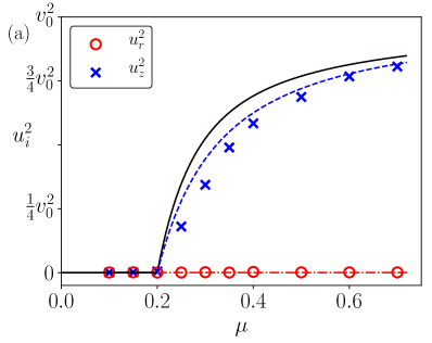
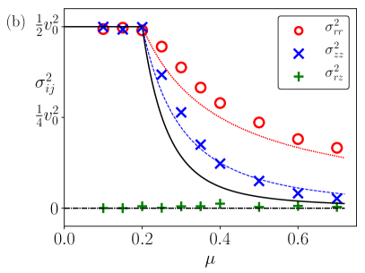
Figure 7: (a): Squared average velocities from simulations as symbols and according to Eq.(35) as black line and according to Eq.(52) as blue dashed line. The red dashed dotted line corresponds to $u_{r}=0$. The critical value for the bifurcation is $\mu_{\text{crit}}=0.2$. (b): Variances and covariance from simulations (symbols). Black line is the expectation value of the orbital variance obtained from the von Mises density and according to Eq.(53) as blue dashed line, according to Eq. (46) as red dotted line as dashed line and according to $\sigma^{2}_{rz}=0$ as dashed dotted line. Parameters: $N=1000$, $v_{0}=1$, $\kappa=1$, $\sigma^{2}=0.1$, $r_{\text{sens}}=0.2$.

For $\mu>\mu_{\text{crit}}$, here $\mu_{\text{crit}}=0.2$, the solution $u_{z}=0$ becomes unstable and two symmetric solutions $u_{z}\neq 0$ are stable. The individual foraging motion turns to cooperative circular motion. In the two dimensional $(x,y)$ plane the searchers start rotating around the home corresponding to the right of Fig.4. While the mean orbital velocity $u_{z}$ seems to be better approximated by the dashed line than by the solid line derived from the von Mises density, we point out, that this might be only the consequence from the simulation of a limited number of particles ($N=1000$).

In Fig. 7(b), we show that our analytical results for the variances Eq. (46) as red dotted line, Eq.(53) as dashed line, the result obtained from the von Mises density as black solid line and the covariance as dashed dotted line at zero approximate the simulation results as symbols reasonably well. At the critical value of the coupling for the alignment the variances start decaying. Here, also the variance $\sigma^{2}_{zz}$ seems to be better approximated by the blue dashed dotted line than the black solid line, but this might be a result of simulations with finite numbers of particles.

Due to the bifurcation there exist two densities $\rho_{z}$. One for $u_{z}<0$ and the second one for the opposite sign of the velocity. We write $\rho_{z-}$ for the density with the maximum at $z=-\pi/2$.

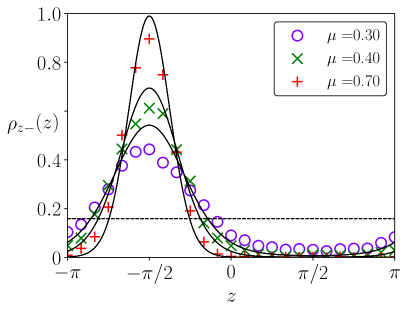
Figure 8: Simulation results for the marginal density of the angle $z$ as symbols and in comparison as lines the approximation (34) for three different values of the coupling $\mu$. The simulation results were chosen for $u_{z}<0$, meaning clockwise rotation in the $(x,y)$ plane. For counterclockwise rotation the densities are shifted by $\pi$. All three values for the coupling are chosen $\mu>\mu_{\text{crit}}=0.2$. The dashed line corresponds to a uniform density. This density is approached for $\mu=\mu_{\text{crit}}$. Deviation from the theoretical value are largely to limited number $N$ of simulated searchers. Parameters: $N=1000$, $v_{0}=1$, $\kappa=1$, $\sigma^{2}=0.1$, $r_{\text{sens}}=0.2$.

We show in Fig.8 simulation results for the density $\rho_{z-}$ as symbols for three different values of the coupling $\mu$. For the simulations results the positions of the particles are ignored as our analytical also is space independent. As lines we present the corresponding von Mises density (34). The dashed line corresponds to a uniform density $\rho_{z}=1/(2\pi)$. This limit is achieved for $\mu=\mu_{\text{crit}}=0.2$ and can be seen in Fig.6. The simulation results are chosen only from steady states where the searchers rotate clockwise in the $(x,y)$ plane. The density (34) was chosen correspondingly. For counterclockwise rotation the densities are shifted by $\pi$. The von Mises density approximates the overall space independent angular density from the simulation well.

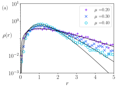
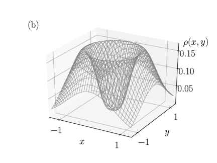
Figure 9: (a): Steady state spatial density for searchers with alignment for different different alignment strength $\mu$. The critical value is $\mu_{\text{crit}}=0.2$. Symbols according to simulations of $N=2000$ searchers. Lines according to Eq. (48). (b): Spatial density for the $(x,y)$ plane. For the coupling a value of $\mu=0.7$ was chosen. While for vanishing alignment the density in the $(x,y)$ plane is maximal at the origin, with an alignment strength large than the critical value the density vanishes at the origin. Parameters: $v_{0}=1$, $\kappa=1$, $\sigma^{2}=0.1$, $r_{\text{sens}}=0.2$.

Finally, we show in Fig.9 the spatial density derived from simulations as symbols and the analytical result from (48) as line. The value for the alignment strength of $\mu=0.2=\mu_{\text{crit}}$ corresponds transition value. Simulation and theory agree well for all displayed values of alignment strength up to a distance of approximately $r\approx 3$. At this distance the simulation results deviate from the theory. This is due to the finite number of simulated searchers, i.e. $N=2000$. At distances $r>3$ the searchers rarely interact with each other due to low density, while for the theory we assumed infinite particle numbers. Parameters are given in the capture of the figure. In Fig. 9(b), we show the result for the marginal density of the position in the $(x,y)$ plane, pointing out that for $\mu>\mu_{\text{crit}}$, here chosen $\mu=0.7>\mu_{\text{crit}}=0.2$, the density at the center decays with increasing $\mu$. The parameters for this figure are as given in the caption.

VI Conclusion

We have studied the transition from individual motion to collective motion for an ensemble of coupled local searchers. Individually, each forager follows a simple version of a path integrating scenario given by a recently proposed search and return dynamics (Noetel et al., 2018a). The searchers of the ensemble move with constant speed and were coupled via an interaction which aligns their heading directions. The latter models the possibility of the foragers to avoid collisions and might for instance result from a drag force of the comoved fluid around the searcher. As a experimental situation for which our model can apply we mention Daphnia moving around an attracting light shaft playing the role of a common home. Former studies on the transition from individual to cooperative trajectories were restricted to computer simulations Erdmann and Ebeling (2009); Vollmer et al. (2006); Mach and Schweitzer (2007); Levine et al. (2001); Thouma et al. (2010). Studies describing midges swarms Gorbonos et al. (2016); Reynolds et al. (2017); Reynolds (2018) do not consider transitions between individual and collective behavior.

Here we give a profound analytical analysis based on a kinetic theory of an ensemble of searchers. Outgoing from a nonlinear FPE (IV.1) we derive nonlinear transport equations and make a detailed bifurcation analysis of the latter.

The situation with a central position also reminisces of models with binary attractive forces between active particles Erdmann et al. (2005); Strefler et al. (2008); Romanczuk et al. (2012) where the common center of mass assumes the role of the central position. But with binary interactions, this position is not fixed in space and might diffuse due the existence of a Goldstone mode, whereas the home in the current investigation is fixed.

The important different point in our investigation compared to the large number of previous analytical, generic studies on collective swarming behavior of self moving units is the existence of a fixed central position, similar to a central field created by the particles but the central place does not shift. The existence of such a central attractive location is quite similar to the existence of external fields Enculescu and Stark (2011); Gorbonos et al. (2016); Reynolds et al. (2017); Reynolds (2018). It prevents a propagation of a swarm along fixed directions as often found in swarming situations. As consequence of the aligning interaction a rotation of the entities around their central position is obtained as collective behavior.

In the paper we found a good agreement for the nonequilibrium phase transition between the numerical simulations and the analytic expressions. Qualitatively, the undercritical situation does not reflect the interactions between particles. Nevertheless it might be worth to investigate correlations between the searchers despite the absence of collective order as recently reported and discussed for swarms of midges Attanasi et al. (2014a, b); Reynolds (2018). In the undercritical situation qualitatively maintain trajectories of the single forager model, while for overcritical coupling trajectories change to circular motion.

In our analysis the marginal density of the distance $\rho(r)$ is the single value which exhibits asymptotically a space dependence. The other characteristics as the mean orbital and radial velocity and their variances get homogeneous in space. The covariance between the two vector components was neglected in agreement with the results of simulations. Except the latter one and the mean radial velocity, all mentioned characteristics change qualitatively their behavior at the critical coupling strength.

We discussed also differences between a decoupling of higher order moments with a von Mises distribution and using a Gaussian decoupling. The first one exhibits a better agreement with the simulations since it was able to reflect the periodicity of the angular variable. Consistently, the two variances of the velocity components differ in their value in case of the von Mises decoupling. We also were able to derive this von Mises distribution for the marginal angular velocity outgoing from the mean field FPE.

The transition from the periodic uniform distribution to a single peaked at critical coupling strength had shown good agreement between simulations and analytics. Similar good agreement was reported for the marginal spatial density $\rho(r)$ of distances from the home. As effect of the alignment this density becomes more narrow around its most probable distance $r_{\text{max}}$. The latter is determined by $r_{\text{max}}=r_{c}=v_{0}/\kappa$ in both under- and over-critical coupling situations. The localization of this peak appears to be independent of the strength $\mu$ between the entities. The contraction of the pdf around $r_{\text{max}}$ reflects the transition from random loops to circular motion of the single searcher.

We also discussed the derivation of a Smoluchowski-equation with under- and the over-critical coupling strength’s. Usually this notion is applied for the kinetics of the pdf of spatial coordinates describing the diffusion of Brownian particles Kramers (1940) in overdamped situations. Therein, the characteristic time scale is larger than the corresponding brake time $\tau_{\gamma}$ of the Brownian particle H’walisz et al. (1989). In our situation, the role of the brake time is taken over by $\tau_{\phi}$. At time scales larger than the angular relaxation time, the inertia of the entities can be neglected which has resulted in the elimination of the angular dynamics. Along these time scales the approximate description of the spatial pdf is given as a diffusion in an external field which is the topic of a Smoluchowski equation.

Our analysis was restricted to values $\mu\leqslant\kappa$. Simulations suggest that for $\mu\geqslant\kappa$ another transition to more exotic flocking patterns appears, where the particles no longer move in circles around the home and the circular symmetry is broken Thouma et al. (2010). Research in such direction also with more complex interaction rules is done in Bonilla and Trenado (2019).

VII Acknowledgement

The authors thank DFG for funding the International research training group 1740 “Dynamical Phenomena in Complex Networks: Fundamentals and Applications” wherein part of the research has been performed. LSG thanks W. Ebeling (Rostock), M. Mazza ( Loughborough) and B. Ronacher (Berlin) for fruitful discussions.

Appendix A Limits of the approximation

While we focused our analysis on the continuum limit of infinite particle numbers and vanishing sensing radius, we numerically investigated the limits of our approximation for the stationary density (48). For this purpose, we varied the particle numbers as well as the sensing radius. An important limiting factor is the number of interacting particles, that means the number of particles within one sensing radius $r_{\text{sens}}$. Even for a rather small total number of simulated particles a transition to a collective rotation around the home can be found. The particles are initially randomly distributed and form over time a persistent rotating cluster.

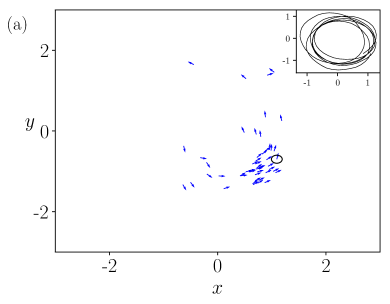
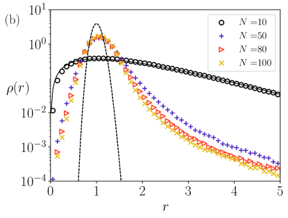
Figure 10: (a): Sample trajectories for a rotating cluster. Total number of particles $N=50$. (b): Spatial densities for different total number $N$ of particles. Symbols according to simulations. Dashed line according to Eq. (48). Solid line according to Eq. (40). Parameters: $\mu=1$, $v_{0}=1$, $\kappa=1$, $\sigma^{2}=0.01$, $r_{\text{sens}}=0.1$.

We present in Fig. 10(a) sample trajectories for such a rotating cluster. The majority of the simulated particles $(N=50)$ is part of the cluster, while some particles follow their own path. The sensing radius is given by $r_{\text{sens}}=0.1$. Correspondingly the spatial density does not follow the undercritical steady state density (40) it slowly starts to approach the steady state density given by (48). This can be seen in Fig. 10(b). Here the total particle number $N$ is varied. For $N=10$ the density (black circles) follows the undercritical or free particles density (40) (line), while for $N=50$ the simulation results (blue plus) for the density already clearly deviates from the undercritical density and approaches the overcritical density (dashed line). With increasing the particle numbers the overcritical density is further approached. Although the particles form a rotating cluster the ensemble average of several simulations has still rotational symmetry around the home.

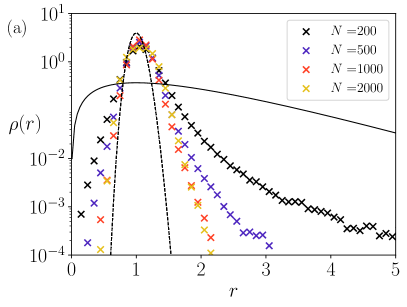
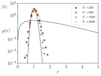
Figure 11: (a): Normalized spatial densities for different total number $N$ of particles. (b): Normalized spatial densities for different total number $N$ of particles with only particles with more than 1 neighbors considered. Symbols according to simulations. Dashed line according to Eq. (48). Solid line according to Eq. (40). Parameters: $\mu=1$, $v_{0}=1$, $\kappa=1$, $\sigma^{2}=0.01$, $r_{\text{sens}}=0.05$.

As already mentioned the number of interacting neighbors is important for the validity of the FPE (IV.1) and its derivations. In order to clarify this aspect we show in Fig. 11 spatial densities for particle numbers $N$ between $200$ and $2000$ but significantly smaller sensing radius than in the previous figures, i.e. $r_{\text{sens}}=0.05$. In (a), we show the spatial densities as before. With increasing total particle number the simulation results approach the derived overcritical density. In (b) however we only consider particles with more than one interacting neighbor and plot their normalized density. For these particles the derivations of the FPE (IV.1), especially the spatial density (48) (dashed line) are valid.

Appendix B Gaussian decoupling of higher moments

In this appendix we show results from a Gaussian decoupling of the third order velocity moments. Writing $v_{0}\cos(z)=u_{r}+\delta u_{r}$ with the first moment is $u_{r}$, the variance reads as $\sigma_{rr}^{2}\rho=\langle\delta u_{r}^{2}\rangle$. In an analog way one defines $v_{0}\sin(z)=u_{z}+\delta u_{z}$ and one obtains the variance $\sigma_{zz}^{2}$ and the covariance. Specifically in the Gaussian approximation, we will neglect the third central moment of the two velocity components. In particular, we will put $\langle\delta u_{r}^{3}\rangle,\langle\delta u_{z}^{3}\rangle\approx 0$. All other third order moments are expressed by products of the two first moments.

The equations for the mean velocities do not change and are identical with Eqs. (25) and (IV.2). Differences occur for the second moments including the variances. Now the r.h.s. does not vanish as for the von Mises decoupling. We find

$$\frac{\partial}{\partial t}\rho\left(u_{r}^{2}+\sigma^{2}_{rr}\right) \,\approx\, -\frac{\partial}{\partial r}\rho u_{r}\left(u^{2}_{r}+3\sigma^{2}_{rr}\right)+\,2\left(\frac{1}{r}-\frac{1}{r_{c}}\right)\rho u_{r}\left(u_{z}^{2}+\sigma^{2}_{zz}\right)$$ (62)

$$+\frac{2\mu}{v_{0}^{2}}\rho\left(u_{r}^{2}\sigma^{2}_{zz}-u_{z}^{2}\sigma^{2}_{rr}\right)+\frac{4\sigma^{2}}{v_{0}^{2}}\left(\frac{\rho v_{0}^{2}}{2}-\rho\left(u_{r}^{2}+\sigma_{rr}\right)\right).$$

and we neglected the third central moments $\langle\delta u_{r}^{3}\rangle$. The orbital energy balance becomes

$$\frac{\partial}{\partial t}\rho\left(u_{z}^{2}+\sigma^{2}_{zz}\right) \,\approx\, -\frac{\partial}{\partial r}\rho u_{r}\left(u_{z}^{2}+\sigma^{2}_{zz}\right)-\,2\left(\frac{1}{r}-\frac{1}{r_{c}}\right)\rho u_{r}\left(u_{z}^{2}+\sigma^{2}_{zz}\right)$$ (63)

$$-\frac{2\mu}{v_{0}^{2}}\rho(u_{r}^{2}\sigma^{2}_{zz}-u_{z}^{2}\sigma^{2}_{rr})+\frac{4\sigma^{2}}{v_{0}^{2}}\left(\frac{\rho v_{0}^{2}}{2}-\rho\left(u_{z}^{2}+\sigma_{zz}\right)\right).$$

Eventually we formulate the equation for the mixed second moment

$$\frac{\partial}{\partial t}\rho u_{r}u_{z} \,\approx\, -\frac{\partial}{\partial r}\rho u_{z}\left(u^{2}_{r}+\sigma^{2}_{rr}\right)+\,2\left(\frac{1}{r}-\frac{1}{r_{c}}\right)\rho u_{z}\left(u_{z}^{2}+3\sigma^{2}_{zz}-\left(u_{r}^{2}+\sigma_{rr}\right)\right)$$ (64)

$$+\frac{2\mu}{v_{0}^{2}}\rho u_{r}u_{z}\left(\sigma^{2}_{zz}+\sigma^{2}_{rr}\right)-\frac{4\sigma^{2}}{v_{0}^{2}}\rho u_{r}u_{z}\,.$$

We now discuss the asymptotic long time behavior of the introduced moments using the Gaussian decoupling. Asymptotically, the marginal density becomes stationary $\rho(r,t)\to\rho(r)$. In accordance with the continuity equation and no-flux boundary conditions the radial flux $u_{r}$ has to vanish $u_{r}=0$. The equation for the radial energy balance simplifies to

$$\frac{\partial\sigma^{2}_{rr}}{\partial t}\,=\,\frac{4\sigma^{2}}{v_{0}^{2}}\left(\frac{v_{0}^{2}}{2}-\sigma^{2}_{rr}\left(1+\frac{\mu}{2\sigma^{2}}u_{z}^{2}\right)\right)\,.$$ (65)

Asymptotically, the radial variance becomes also stationary and homogeneous in space. We set the l.h.s. to zero and get the algebraic equation

$$\sigma^{2}_{rr}\,=\,\frac{v_{0}^{2}}{2\left(1+\frac{\mu}{2\sigma^{2}}u_{z}^{2}\right)}\,.$$ (66)

Insertion of this variance yields the stationary solutions of $u_{z}$ which obey the equation

$$0=\left(\frac{\mu}{2\left(1+\frac{\mu}{2\sigma^{2}}u_{z}^{2}\right)}-\left(\frac{\sigma}{v_{0}}\right)^{2}\right)u_{z}.$$ (67)

Solutions of this equation exhibit a pitchfork bifurcation. The mean orbital velocity of the coupled searchers vanishes asymptotically $u_{z}=0$ which is stable for a coupling strength smaller than the critical value $\mu\leqslant\mu_{c}$. The expression for the critical coupling strength coincides with the value of the von Mises decoupling (36). Likewise in the former under-critical case, the variances in this state follow from Eqs.(63) and (66)

$$\sigma^{2}_{rr}\,=\,\sigma^{2}_{zz}\,=\,\frac{v_{0}^{2}}{2}\,.$$ (68)

The r.h.s of the equation for the mixed second moment (64) vanishes and the equation for the radial flux (25) results in the stationary Smoluchowski-equation (57) for the marginal density with the solution (40).

In contrast, the situation differs for coupling strengths $\mu\geqslant\mu_{c}$ larger than the critical value (36). The non-vanishing orbital velocity becomes in the Gaussian approximation

$$u_{z}\,=\,\pm v_{0}\sqrt{1-\frac{\mu_{c}}{\mu}}\,=\,\pm v_{0}\sqrt{1-\frac{2\sigma^{2}}{\mu}}\,.$$ (69)

In this state the variances coincide again and behave thus differently from the von Mises decoupling and the simulations. Both become

$$\sigma^{2}_{rr}\,=\,\sigma^{2}_{zz}\,=\,\frac{v_{0}^{2}}{2}\,\frac{\mu_{c}}{\mu}\,=\,\frac{\sigma^{2}}{\mu}.$$ (70)

They vanish for strong coupling where all kinetic energy is contained in the mean orbital motion since $u^{2}_{z}=v^{2}_{0}$.

In result, the main difference between the two decoupling scenarios consists in the different partition of kinetic energy at the orbital degree of freedom. We point out that the results of the von Mises decoupling fit better with the numerical findings than those from the Gaussian decoupling. The radial component of the energy equals in both decoupling scenarios. The orbital variance equals the radial variance in the Gaussian decoupling.

However, in the von Mises decoupling more energy is spend to the systematic orbital motion $u_{z}^{2}$ and less energy to its fluctuation $\sigma_{zz}^{2}$. It is a consequence of the less broad von Mises distribution compared to its Gaussian counterpart.

In detail, in the Gaussian decoupling we get for the third order moment in the energy balance

$$\frac{\mu}{v_{0}^{2}}u_{z}\langle v_{0}^{3}\cos^{2}(z)\sin(z)\rangle\,\approx\,\frac{\mu}{v_{0}^{2}}u_{z}^{2}\sigma_{rr}^{2}\,.$$ (71)

The same moment approximated with the von Mises decoupling as

$$\frac{\mu}{v_{0}^{2}}u_{z}\langle v_{0}^{3}\cos^{2}(z)\sin(z)\rangle\,\approx\,\frac{\sigma^{2}}{v_{0}^{2}}\left(u_{z}^{2}+\sigma_{zz}^{2}-\sigma_{rr}^{2}\right)\,.$$ (72)

But, remarkably, the third moment as a solution of the two differently decoupled transport equations possesses the same expression. In both cases it becomes asymptotically

$$\frac{\mu}{v_{0}^{2}}u_{z}\langle v_{0}^{3}\cos^{2}(z)\sin(z)\rangle\,\approx\,\frac{\sigma^{2}}{v_{0}^{2}}\left(v_{0}^{2}-\frac{2\sigma^{2}}{v_{0}^{2}}\right)\,,$$ (73)

But whereas the Gaussian decoupling relies on the asymptotic values of the mean orbital velocity $u_{z}$ from (69) and the variance $\sigma_{rr}$ from (70), we made use in the von Mises scheme from $u_{z}$ given by (52) and its variances, $\sigma_{zz}$ from (53) and $\sigma_{rr}$ from (46).

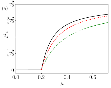
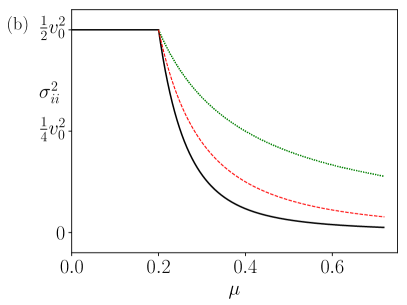
Figure 12: Comparison of the analytical results of the two decoupling schemes. (a): Squared average velocities according to the decoupling using the von Mises distribution Eq.(35) (black, line), Eq.(52) (red, dashed) and to the Gaussian decoupling (69) (green, dotted). All nonvanishing mean orbital velocities appear at the same critical value for the bifurcation which is in the particular case $\mu_{\text{crit}}=0.2$. (b): Orbital variances obtained from the von Mises density (black, line) and according to Eq.(53) (red, dashed) and Eq. (46) (green, dotted). Both Gaussian counterparts coincides with each other, and with variance of the radial velocity fluctuations of the von Mises decoupling scenario. The Gaussian variances does not account that the orbital velocity fluctuations possess a smaller variance. Parameters: $N=1000$, $v_{0}=1$, $\kappa=1$, $\sigma^{2}=0.1$.

With the Gaussian decoupling the stationary marginal radial density $\rho(r)$ obeys the same Smoluchowski equation as in the case of the decoupling by help of the von Mises distribution. Insertion of the steady states for $u_{z}^{2},\sigma^{2}_{rr}$ and $\sigma^{2}_{zz}$ into Eq.(25) results in

$$0=\frac{\sigma^{2}}{\mu}\frac{\partial}{\partial r}\left\{\frac{\partial}{\partial r}-\left(\frac{1}{r}-\frac{\kappa}{v_{0}}\right)\left(\frac{\mu v_{0}^{2}}{\sigma^{2}}-1\right)\right\}\rho(r)\,,$$ (74)

which possesses the solution (48). Thus, the von Mises decoupling improves only the orbital characteristics of the studied problem.

Appendix C Mechanics of the searcher

The search and return mechanism of a single searcher Eqs. (1) and (2) allow a mechanical interpretation at the two dimensional plane (see Fig.1). We formulate the Newton law of mechanics

$$\frac{{\rm d}}{{\rm dt}}\,\vec{v}\,=\,\gamma\left(v_{0}\vec{e}_{v}\,-\,\vec{v}\right)\,-\,k\vec{e}_{r}\,.$$ (75)

for the two dimensional motion of a particle. The latter is damped by Stokes friction with coefficient $\gamma$ and pushed by an internal motor with strength $\gamma v_{0}$. The velocity vector is $\vec{v}(t)=v(t)\vec{e}_{v}$ with speed $v(t)$, heading direction $\phi(t)$ and unit velocity vector $\vec{e}_{v}(t)=\{\cos(\phi(t)),\sin(\phi(t))\}$. Additionally, a central constant attractive force acts along the unit vector of the position vector $\vec{e}_{r}(t)=\{\cos(\beta(t),\sin(\beta(t))\}$ with orientation given by the angle $\beta(t)$. The force is independent of the distance $r(t)$ from the home and depends only on $\beta(t)$.

Now we allow infinitely large damping $\gamma\to\infty$ as considered in the overdamped limit. Projection on the speed and heading variables gives

$$\vec{v}(t)\,=\,v_{0}\,\vec{e}_{v}(t)\,.$$ (76)

We assumed that the limit $k/\gamma$ vanishes for large damping. The situation reduces to a microswimmer with constant speed.

Alternatively, the heading dynamics reads

$$\dot{\phi}\,=\,\frac{k}{v_{0}}\,\sin(\phi-\beta)\,,$$ (77)

with $\kappa=k/v_{0}$. We got Eq. (2) and, thus, the path integration program has been traced back from a mechanical problem given by the Newton law (75) and formulating mechanical forces. During the path integration the searcher is always aware of the direction towards the home without having knowledge about the distance.

An alternative interesting model was recently proposed by Waldner and Merkle Waldner and Merkle (2018). It considers a central harmonic force and recovers beautiful rosette like trajectories around the home which have been reported several times for dessert ants Mittelstaedt and Mittelstaedt (1980); Vickerstaff and Di Paolo (2005); Ronacher (2008); Collett et al. (2013). Formally, one should replace $k\to k_{0}*r(t)$ in (75) and, subsequently, in(77).

To take $k$ as a function of the distance might be a fruitful direction to get better agreement with experimentally found trajectories. One could consider general central forces with a distant dependent $k(r)$ in (75) and will get the same $k(r)$ in the heading dynamics (2). Some particular cases have been investigated in Noetel et al. (2018a). Therein, the deterministic case well as the stationary stochastic problem with added angular noise in the $\phi$-dynamics have been analytically solved.

References

References

- Klages (2017) R. Klages, “Search for Food of Birds, Fish and Insects,” in Diffusive Spreading in Nature, Technology and Society, edited by A. Bunde, J. Caro, J. Kärger, and G. Vogl (Springer, Cham, 2017) pp. 49–69.
- Mittelstaedt and Mittelstaedt (1980) M. Mittelstaedt and H. Mittelstaedt, Naturwissenwschaften 67, 566 (1980).
- Bénichou et al. (2011) O. Bénichou, C. Loverdo, M. Moreau, and R. Voituriez, Rev. Mod. Phys. 83, 81 (2011).
- Cheng (1995) K. Cheng, in Psychology of Learning and Motivation, Psychology of Learning and Motivation, Vol. 33 (Academic Press, 1995) pp. 1 – 21.
- Wang (2003) R. F. Wang, in Cognitive Vision, Psychology of Learning and Motivation, Vol. 42 (Academic Press, 2003) pp. 109 – 156.
- Seelig and Jayaraman (2015) J. D. Seelig and V. Jayaraman, Nature 521, 186 (2015).
- Green et al. (2017) J. Green, A. Adachi, K. K. Shah, J. D. Hirokawa, P. S. Magani, and G. Maimon, Nature 546, 101 (2017).
- Zeil (2012) J. Zeil, Cur. Opinion in Neurobiology 22, 285 (2012).
- Wehner and Srinivasan (1981) R. Wehner and M. V. Srinivasan, Journal of Comparative Physiology A 142, 315 (1981).
- Ronacher (2008) B. Ronacher, Myrmecological News 11, 53 (2008).
- Collett et al. (2013) M. Collett, L. Chittka, and T. S. Collett, Current Biology 23, R789 (2013).
- el Jundi (2017) B. el Jundi, Current Biology 27, R748 (2017).
- Kim and Dickinson (2017) I. S. Kim and M. H. Dickinson, Current Biology 27, 2227 (2017).
- Wehner et al. (1996) R. Wehner, B. Michel, and P. Antonsen, Journal of Experimental Biology 199, 129 (1996).
- Vickerstaff and Di Paolo (2005) R. J. Vickerstaff and E. A. Di Paolo, in Advances in Artificial Life, edited by M. S. Capcarrère, A. A. Freitas, P. J. Bentley, C. G. Johnson, and J. Timmis (Springer Berlin Heidelberg, Berlin, Heidelberg, 2005) pp. 221–230.
- Vickerstaff and Merkle (2012) R. J. Vickerstaff and T. Merkle, Journal of Theoretical Biology 307, 1 (2012).
- Waldner and Merkle (2018) F. Waldner and T. Merkle, Journal of Comparative Physiology A 204, 985 (2018).
- Chien and Wagstaff (2017) S. Chien and K. L. Wagstaff, Science Robotics 2 (2017).
- Hook et al. (2013) J. V. Hook, P. Tokekar, E. Branson, P. G. Bajer, P. W. Sorensen, and V. Isler, “Local-Search Strategy for Active Localization of Multiple Invasive Fish,” in Experimental Robotics: The 13th International Symposium on Experimental Robotics, edited by J. P. Desai, G. Dudek, O. Khatib, and V. Kumar (Springer International Publishing, Heidelberg, 2013) pp. 859–873.
- Girdhar et al. (2011) Y. Girdhar, A. Xu, B. B. Dey, M. Meghjani, F. Shkurti, I. Rekleitis, and G. Dudek, IEEE/RSJ , 5048 (2011).
- Leonard et al. (2007) N. Leonard, D. Paley, F. Lekien, R. Sepulchre, D. Fratantoni, and R. Davis, Proceedings of the IEEE 95, 48 (2007).
- Dubowsky et al. (2005) S. Dubowsky, K. Iagnemma, S. Liberatore, D. Lambeth, J. Plante, and P. J. Boston, Space Technology International Forum , 1449 (2005).
- Duarte et al. (2016) M. Duarte, V. Costa, J. Gomes, T. Rodrigues, F. Silva, S. M. Oliveira, and A. L. Christensen, PLOS ONE 11, 1 (2016).
- Nirmal and Lyons (2016) P. Nirmal and D. Lyons, Robotica 34, 2741 (2016).
- Möller et al. (2001) R. Möller, D. Lambrinos, T. Roggendorf, and R. P. R. Wehner, “Insect Strategies of Visual Homing in Mobile Robots,” in Biorobotics. Methods and Applications, edited by B. Webb and T. R. Consi (AAAI Press / MIT Press, 2001) pp. 37–66.
- Noetel et al. (2018a) J. Noetel, V. L. S. Freitas, E. E. N. Macau, and L. Schimansky-Geier, Phys. Rev. E 98, 022128 (2018a).
- Noetel et al. (2018b) J. Noetel, V. L. S. Freitas, E. E. N. Macau, and L. Schimansky-Geier, Chaos 28, 106302 (2018b).
- Okubo (1986) A. Okubo, Advances in Biophysics 22, 1 (1986).
- Gorbonos et al. (2016) D. Gorbonos, R. Ianconescu, J. G. Puckett, R. Ni, N. T. Ouellette, and N. S. Gov, New Journal of Physics 18, 073042 (2016).
- Reynolds et al. (2017) A. M. Reynolds, M. Sinhuber, and N. T. Ouellette, The European Physical Journal E 40, 46 (2017).
- Reynolds (2018) A. M. Reynolds, Journal of The Royal Society Interface 15 (2018), 10.1098/rsif.2017.0806.
- Schweitzer and Schimansky-Geier (1994) F. Schweitzer and L. Schimansky-Geier, Physica A 206, 359 (1994).
- Chavanis (2014) P.-H. Chavanis, The European Physical Journal B 87, 120 (2014).
- Delcourt et al. (2016) J. Delcourt, N. Bode, and M. Denoél, The Quarterly Review of Biology 91, 1 (2016).
- Ordemann (2002) A. Ordemann, Biol. Physicist 2, 5 (2002).
- Ordemann et al. (2003a) A. Ordemann, G. Balazsi, and F. Moss, Physica A: Statistical Mechanics and its Applications 325, 260 (2003a).
- Ordemann et al. (2003b) A. Ordemann, G. Balaszi, and F. Moss, Nova Acta Leopoldina 88, 87 (2003b).
- Erdmann et al. (2004) U. Erdmann, W. Ebeling, L. Schimansky-Geier, A. Ordemann, and F. Moss, arXiv:q-bio 325, 0404018 (2004).
- Garcia et al. (2007) R. Garcia, F. Moss, A. Nihongi, J. Strickler, S. Göller, U. Erdmann, L. Schimansky-Geier, and I. Sokolov, Mathematical Biosciences 207, 165 (2007).
- Dees et al. (2008) N. Dees, S. Bahar, and F. Moss, Physical Biology 5, 044001 (2008).
- Erdmann and Ebeling (2009) U. Erdmann and W. Ebeling, Fluctuation and Noise Letters 3, L145 (2009).
- Vollmer et al. (2006) J. Vollmer, A. Vegh, C. Lange, and B. Eckhardt, Physical Review E 73, 061924 (2006).
- Mach and Schweitzer (2007) R. Mach and F. Schweitzer, Bulletin of Mathematical Biology 69, 539 (2007).
- Levine et al. (2001) H. Levine, W.-J. Rappel, and I. Cohen, Physical Review E 63, 017101 (2001).
- Strefler et al. (2008) J. Strefler, U. Erdmann, and L. Schimansky-Geier, Physical Review E 78, 031927 (2008).
- Thouma et al. (2010) J. Thouma, A. Shreim, and L. Klushin, Physical Review E 81, 066106 (2010).
- Okubo and Levin (2002) A. Okubo and S. Levin, Diffusion and Ecological Problems: Modern Perspectives (Springer, Berlin, 2nd ed., 2002) interdisciplinary Applied Mathematics Vol.14.
- Vicsek et al. (1995) T. Vicsek, A. Czirók, E. Ben-Jacob, I. Cohen, and O. Shochet, Phys. Rev. Lett. 75, 1226 (1995).
- Chaté et al. (2008a) H. Chaté , F. Ginelli, G. Grégoire, and F. Raynaud, Physical Review E 77, 046113 (2008a).
- Chaté et al. (2008b) H. Chaté , F. Ginelli, G. Grégoire, F. Peruani, and F. Raynaud, European Physical Journal B 64, 451 (2008b).
- Peruani et al. (2008) F. Peruani, A. Deutsch, and M. Bär, European Physical Journal Special Topics 157, 111 (2008).
- Romanczuk et al. (2012) P. Romanczuk, M. Bär, W. Ebeling, B. Lindner, and L. Schimansky-Geier, European Physical Journal Special Topics 202, 1 (2012).
- Vicsek and Zafeiris (2012) T. Vicsek and A. Zafeiris, Physics Reports 517, 71 (2012).
- Großmann et al. (2014) R. Großmann, P. Romanczuk, M. Bär, and L. Schimansky-Geier, Phys. Rev. Lett. 113, 258104 (2014).
- Kuramoto (1984) Y. Kuramoto, Chemical Oscillations, Waves, and Turbulence (Springer-Verlag, New York, 1984).
- Pikovsky et al. (2001) A. Pikovsky, M. Rosenblum, and J. Kurths, Synchronization: A universal concept in nonlinear sciences (Pres Syndicate of the University of Cambridge, Cambridge, 2001).
- Lauga and Powers (2009) E. Lauga and T. Powers, Reports on Progress in Physics 72, 096601 (2009).
- Downton and Stark (2009) M. T. Downton and H. Stark, Journal of Physics: Condensed Matter 21, 204101 (2009).
- Schwarzendahl and Mazza (2018) F. Schwarzendahl and M. Mazza, Soft Matter 14, 4666 (2018).
- Schwarzendahl and Mazza (2019) F. Schwarzendahl and M. Mazza, The Journal of Chemical Physics 150, 184902 (2019).
- Russel and Norvig (2010) S. J. Russel and P. Norvig, The Organization of Learning (The MIT Press, Cambridge MA, US, 2010).
- Mittelstaedt (1962) H. Mittelstaedt, Annual Review of Entomology 7, 177 (1962).
- Forucassie and Traniello (1994) V. Forucassie and J. Traniello, Animal Behavior 48, 69 (1994).
- Freska and Mark (1999) C. Freska and D. Mark, Spatial Information Theory, Vol. 1661 (Springer, Berlin, 1999).
- Vickerstaff and Cheung (2010) R. Vickerstaff and A. Cheung, Journal of Theoretical Biology 263, 242 (2010).
- Hoffmann (1983) G. Hoffmann, Behavioral Ecology and Sociobiology 13, 81 (1983).
- Wehner et al. (2002) R. Wehner, K. Gallizzi, C. Frei, and M. Vesely, J. Comp. Physiol. A 188, 683 (2002).
- Collett (2010) M. Collett, Proceedings of the National Academy of Science USA 107, 11638 (2010).
- Capaldi et al. (2000) E. Capaldi, J. Smith, A.D. ad Osborne, S. Fahrbach, S. Farris, D. Reynolds, A. Edwards, A. Martin, G. Robinson, G. Poppy, and J. Riley, Nature 403, 537 (2000).
- Osborne et al. (2013) J. Osborne, A. Smith, S. Clark, D. Reynolds, M. Barron, K. Lim, and A. Reynolds, PLOS One 8, e78681 (2013).
- Reynolds et al. (2007a) A. Reynolds, A. Smith, U. Greggers, D. Reynolds, and J. Riley, Ecology 88, 1955 (2007a).
- Reynolds et al. (2007b) A. Reynolds, A. Smith, D. Reynolds, N. Carreck, and J. Osborne, Journal of Experimental Biology 210, 3763 (2007b).
- Lenz et al. (2013) F. Lenz, A. Chechkin, and R. Klages, PLOS One 8, e59036 (2013).
- Collett (2000) T. Collett, Nature 403, 488 (2000).
- Makinson et al. (2019) J. Makinson, J. Woodgate, A. Reynolds, E. Capaldi, J. Clint, and L. Chittka, Scientific Reports 9, 4651 (2019).
- Mikhailov and Meinköhn (1997) A. Mikhailov and D. Meinköhn, in Stochastic Dynamics, edited by L. Schimansky-Geier and T. Pöschel (Springer Berlin Heidelberg, Berlin, Heidelberg, 1997) pp. 334–345.
- Nötel et al. (2017) J. Nötel, I. M. Sokolov, and L. Schimansky-Geier, Journal of Physics A: Mathematical and Theoretical 50, 034003 (2017).
- Stratonovich (1967) R. Stratonovich, Topics in the Theory of Random Noise, Vol. II (Gordon and Breach, Science publisher, New York, 1967) p. 234ff.
- Kürsten and Ihle (2017) R. Kürsten and T. Ihle, Journal of Statistical Mechanics: Theory and Experiment 2017/3, 033202 (2017).
- Slater (1959) J. Slater, Physical Review 81, 385 (1959).
- Balescu (1960) R. Balescu, The Physics of Fluids 3, 52 (1960).
- Mukamel et al. (1978) S. Mukamel, I. Proccacia, and J. Ross, The Journal of Chemical Physics 68, 1205 (1978).
- Stanley (1971) H. Stanley, Mean Field Theory of Magnetic Phase Transitions (Phenomena. Oxford University Press, 1971).
- Kadanoff (2009) L. P. Kadanoff, Jounral of Statistical Physics , 777 (2009).
- den Broeck et al. (1997) C. V. den Broeck, J. Parrondo, R. Toral, and R. Kawai, Physical Review E 55, 4084 (1997).
- Sagués et al. (2007) F. Sagués, J. Sancho, and J. García-Ojalvo, Review of Modern Physics 79, 829 (2007).
- Strogatz (2000) S. H. Strogatz, Physica D 143, 1 (2000).
- Bonilla and Trenado (2018) L. Bonilla and C. Trenado, Physical Review E 98, 062603 (2018).
- Erdmann et al. (2005) U. Erdmann, W. Ebeling, and A. Mikhailov, Physical Review E 71, 051904 (2005).
- Enculescu and Stark (2011) M. Enculescu and H. Stark, Physical Review Letters 107, 058301 (2011).
- Attanasi et al. (2014a) A. Attanasi, A. Cavagna, L. Del Castello, S. Giardina, S. Melillo, L. Parisi, O. Pohl, B. Rossaro, E. Shen, E. Silvestri, and M. Viale, Physical Review Letters 113, 238102 (2014a).
- Attanasi et al. (2014b) A. Attanasi, A. Cavagna, L. Del Castello, S. Giardina, S. Melillo, L. Parisi, O. Pohl, B. Rossaro, E. Shen, E. Silvestri, and M. Viale, PLOS Computational Biology 10, e1003697 (2014b).
- Kramers (1940) H. Kramers, Physica 7, 284 (1940).
- H’walisz et al. (1989) L. H’walisz, P. Jung, P. Hänggi, P. Talkner, and L. Schimansky-Geier, Zeitschrift für Physik B Condensed Matter 77, 471 (1989).
- Bonilla and Trenado (2019) L. Bonilla and C. Trenado, Physical Review E 99, 012612 (2019).