PDM-charged particles in PD-magnetic plus Aharonov-Bohm flux fields: unconfined ”almost-quasi-free” and confined in a Yukawa plus Kratzer exact solvability

Abstract

Abstract: Using azimuthally symmetrized cylindrical coordinates, we consider some position-dependent mass (PDM) charged particles moving in position-dependent (PD) magnetic and Aharonov-Bohm flux fields. We focus our attention on PDM-charged particles with $m\left(\overrightarrow{r}\right)=g\left(\rho\right)=\eta\,f\left(\rho\right)\exp\left(-\delta\rho\right)$ (i.e., the PDM is only radially dependent) moving in an inverse power-law-type radial PD-magnetic fields $\overrightarrow{B}=B_{\circ}\left(\mu/\rho^{\sigma}\right)\widehat{z}$. Under such settings, we consider two almost-quasi-free PDM-charged particles (i.e., no interaction potential, $V\left(\overrightarrow{r}\right)=0$) endowed with $g\left(\rho\right)=\eta/\rho$ and $g\left(\rho\right)=\eta/\rho^{2}$. Both yield exactly solvable Schrödinger equations of Coulombic nature but with different spectroscopic structures. Moreover, we consider a Yukawa-type PDM-charged particle with $g\left(\rho\right)=\eta\,\exp\left(-\delta\rho\right)/\rho$ moving not only in the vicinity of the PD-magnetic and Aharonov-Bohm flux fields but also in the vicinity of a Yukawa plus a Kratzer type potential force field $V\left(\rho\right)=-V_{\circ}\exp\left(-\delta\rho\right)/\rho-V_{{}_{1}}/\rho+V_{{}_{2}}/\rho^{2}$. For this particular case, we use the Nikiforov-Uvarov (NU) method to come out with exact analytical eigenvalues and eigenfunctions. Which, in turn, recover those of the almost-quasi-free PDM-charged particle with $g\left(\rho\right)=\eta/\rho$ for $V_{\circ}=V_{{}_{1}}=V_{{}_{2}}=0=\delta$. Energy levels crossings are also reported.

PACS numbers: 03.65.-w, 03.65,Ge, 03.65.Fd

Keywords: position-dependent mass Hamiltonian, cylindrical coordinates, position-dependent magnetic field, Aharonov-Bohm flux field, almost-quasi-free PDM-charged particles, Yukawa-plus-Kratzer potential, Nikiforov-Uvarov exact solvability.

I Introduction

A charged particle moving in a uniform/constant magnetic field and/or an Aharonov-Bohm flux field has been a subject of research interest over the years 1 ; 2 ; 3 ; 4 ; 5 ; 6 ; 7 ; 8 ; 9 ; 10 . On the classical mechanical and mathematical side of the problem, it is crucial to know that the canonical momentum is no longer the mass times velocity but an extra term is added so that $p_{{}_{i}}=m_{\circ}v_{{}_{i}}+eA_{{}_{i}}$ (where $m_{\circ}$ is the conventional constant mass, $e$ is the charge of the particle and $A_{{}_{i}}$ is the $i$th component of the vector potential). The problem is readily of a delicate nature, especially when the magnetic field is no longer a constant but rather a position-dependent one (to be referred to as PD-magnetic field, hereinafter). Moreover, particles endowed with position-dependent mass (PDM) are considered interesting and unavoidable in both quantum and classical mechanics 11 ; 12 ; 13 ; 14 ; 15 ; 16 ; 17 ; 18 ; 19 ; 20 ; 21 ; 22 ; 23 ; 24 ; 25 ; 26 ; 27 ; 28 ; 29 ; 30 ; 31 ; 32 ; 33 ; 34 ; 35 ; 36 . Such mass settings find their applications in condensed matter physics (see, e.g., 20 ; 26 ; 27 ; 30 ), in optical physics (see, e.g., 37 ; 38 ), etc. They are not to be necessarily understood as particles with PDM literally. A position-dependent deformation in the coordinate system may very well render the mass position-dependent. One would then express the mass as $M\left(\overrightarrow{r}\right)=m_{\circ}m\left(\overrightarrow{r}\right)$, where $m\left(\overrightarrow{r}\right)$ is a dimensionless position-dependent scalar multiplier. It would be interesting, therefore, to consider a PDM-charged particle moving in not only a PD-magnetic field and an Aharonov-Bohm flux field but also in the vicinity of a Yukawa-type plus a Kratzer-type molecular interaction force fields. Hereby, we need to use the Nikiforov-Uvarov (NU) method (see e.g. 39 ; 40 ; 41 ) and explore its exact solvability. This forms a constituent inspiration of the current methodical proposal.

A priori, we recollect that while in classical mechanics the PDM particles cause no conflict at all (see, e.g., 31 ; 36 ), they yield an ordering ambiguity problem in quantum mechanics. This ambiguity is a manifestation of the non-unique representation of the PDM kinetic energy operator (see e.g., 12 ; 13 ; 22 ; 24 ; 36 ) of the von Roos Hamiltonian 12 . However, in his analysis on the transition from classical PDM-Hamiltonians into quantum mechanical PDM-Hamiltonians, Mustafa 36 has argued (using $\hbar=2m_{\circ}=1$ units) that whilst it is safe in classical mechanics to write the PDM-kinetic energy term as

$$T=\frac{\overrightarrow{P}\left(\overrightarrow{r}\right)^{2}}{2m\left(\overrightarrow{r}\right)};\text{ \ }\overrightarrow{P}\left(\overrightarrow{r}\right)=m\left(\overrightarrow{r}\right)\vec{v},$$ (1)

it is necessary and convenient to write the quantum mechanical kinetic energy operator as

$$\widehat{T}=\left(\frac{\widehat{P}\left(\overrightarrow{r}\right)}{\sqrt{m\left(\overrightarrow{r}\right)}}\right)^{2}.$$ (2)

Where $\widehat{P}\left(\overrightarrow{r}\right)$ is the PDM-momentum operator. Consequently, the PDM-minimal coupling $\widehat{P}\left(\overrightarrow{r}\right)\longrightarrow\widehat{P}\left(\overrightarrow{r}\right)-e\overrightarrow{A}\left(\overrightarrow{r}\right)$ should be indulged into the PDM-Schrödinger equation  as

$$\left[\left(\frac{\widehat{P}\left(\overrightarrow{r}\right)-e\overrightarrow{A}\left(\overrightarrow{r}\right)}{\sqrt{m\left(\overrightarrow{r}\right)}}\right)^{2}+W\left(\overrightarrow{r}\right)\right]\psi\left(\overrightarrow{r}\right)=E\psi\left(\overrightarrow{r}\right);\ \ W\left(\overrightarrow{r}\right)=e\varphi\left(\overrightarrow{r}\right)+V\left(\overrightarrow{r}\right),$$ (3)

where $\overrightarrow{A}\left(\overrightarrow{r}\right)$ is the vector potential, $e\varphi\left(\overrightarrow{r}\right)$ is a scalar potential and $V\left(\overrightarrow{r}\right)$ is any other potential energy than the electromagnetic one. In a subsequent work, moreover, Mustafa and Algadhi 11 have constructed and defined the PDM-momentum operator as

$$\widehat{P}\left(\overrightarrow{r}\right)=-i\left[\overrightarrow{\nabla}-\frac{1}{4}\left(\frac{\overrightarrow{\nabla}m\left(\overrightarrow{r}\right)}{m\left(\overrightarrow{r}\right)}\right)\right].$$ (4)

This would allow us to re-write equation (3) as

$$\left[-\frac{1}{m\left(\overrightarrow{r}\right)}\overrightarrow{\nabla}^{2}+\left(\frac{\overrightarrow{\nabla}m\left(\overrightarrow{r}\right)}{m\left(\overrightarrow{r}\right)^{2}}\right)\cdot\overrightarrow{\nabla}+\frac{1}{4}\left(\frac{\overrightarrow{\nabla}^{2}m\left(\overrightarrow{r}\right)}{m\left(\overrightarrow{r}\right)^{2}}\right)-\frac{7}{16}\left(\frac{\left[\overrightarrow{\nabla}m\left(\overrightarrow{r}\right)\right]^{2}}{m\left(\overrightarrow{r}\right)^{3}}\right)+\frac{2\ i\ e}{m\left(\overrightarrow{r}\right)}\overrightarrow{A}\left(\overrightarrow{r}\right)\cdot\overrightarrow{\nabla}\right.$$

$$\quad\quad\left.+\frac{ie}{m\left(\overrightarrow{r}\right)}\left(\overrightarrow{\nabla\,}\cdot\overrightarrow{A}\left(\overrightarrow{r}\right)\right)-i\ e\ \overrightarrow{A}\left(\overrightarrow{r}\right)\cdot\left(\frac{\overrightarrow{\nabla}m\left(\overrightarrow{r}\right)}{m\left(\overrightarrow{r}\right)^{2}}\right)+\frac{e^{2}\overrightarrow{A}\left(\overrightarrow{r}\right)^{2}}{m\left(\overrightarrow{r}\right)}+W\left(\overrightarrow{r}\right)\right]\psi\left(\overrightarrow{r}\right)=E\psi\left(\overrightarrow{r}\right),$$ (5)

in which the vector potential takes a conventional form that satisfies the Coulomb gauge $\overrightarrow{\nabla}\cdot\overrightarrow{A}\left(\overrightarrow{r}\right)=0$ and results in a uniform constant magnetic field through the traditional textbook recipe $\overrightarrow{\nabla}\times\overrightarrow{A}\left(\overrightarrow{r}\right)=\overrightarrow{B}=B_{\circ}\widehat{z}$. This magnetic field setting is the commonly and frequently used in the literature (see e.g. 42 and related references cited therein). Nevertheless, in the construction of the vector potential $\overrightarrow{A}\left(\overrightarrow{r}\right)$, the magnetic field may turn out to be a PD-magnetic field (see e.g., 11 ; 43 ). In our current proposal, we focus our attention on PDM-charged particles in PD-magnetic and Aharonov-Bohm flux fields, without the confinement potential (i.e., $V\left(\overrightarrow{r}\right)=0$) and with a confinement potential (i.e., $V\left(\overrightarrow{r}\right)\neq 0$). The organization of this paper is, therefore, in order.

In section 2, we consider a PDM-charged particle in PD-magnetic and Aharonov-Bohm flux fields and discuss the separability of the PDM-Schrödinger equation (5) using azimuthally symmetrized cylindrical coordinates $\left(\rho,\varphi,z\right)$. Therein, we use a general form of the vector potential $\overrightarrow{A}\left(\overrightarrow{r}\right)$ so that a radial PD-magnetic field emerges in the process (i.e., $\overrightarrow{B}=B_{\circ}F\left(\rho\right)\widehat{z}$, where $F\left(\rho\right)$ is a dimensionless radial scalar multiplier to be discussed/determined below). In the same section, moreover, we construct our PD-magnetic field in such a way that it is of a feasibly experimentally applicable nature (i.e., inverse power-law type $\overrightarrow{B}=B_{\circ}\left(\mu/\rho^{\sigma}\right)\widehat{z}$) to be used along with a PDM $m\left(\overrightarrow{r}\right)=g\left(\rho\right)=\eta\,f\left(\rho\right)\exp\left(-\delta\rho\right)$ (i.e., the PDM is only radial-dependent). In section 3, we consider the what may be called almost-quasi-free PDM-charged particles (i.e., no other interaction potential than the interaction of the PDM-charged particles with the PD-magnetic and Aharonov-Bohm flux fields, where the conventional confinement $V\left(\overrightarrow{r}\right)=0$) endowed with two unavoidable exactly solvable PDM models $g\left(\rho\right)=\eta/\rho$ and $g\left(\rho\right)=\eta/\rho^{2}$. A PDM-charged particle, with $m\left(\overrightarrow{r}\right)=g\left(\rho\right)=\eta\,\exp\left(-\delta\rho\right)/\rho$; $f\left(\rho\right)=1/\rho$, interacting with a PD-magnetic plus Aharonov-Bohm flux fields and moving in the vicinity of a Yukawa plus a Kratzer type potential force field $V\left(\rho\right)=-V_{\circ}\exp\left(-\delta\rho\right)/\rho-V_{{}_{1}}/\rho+V_{{}_{2}}/\rho^{2}$ is considered in section 4. Where the Nikiforov-Uvarov (NU) method is used to obtain exact eigenvalue and eigenfunctions. The potency of this method in obtaining exact analytical solutions is well documented in the sample of references (see, e.g., 6 ; 39 ; 40 ; 41 ). Such exact results collapse into those of the almost-quasi-free PDM-charged particles with $m\left(\overrightarrow{r}\right)=g\left(\rho\right)=\eta/\rho$, of section 3, when $V_{\circ}=V_{{}_{1}}=V_{{}_{2}}=0=\delta$ are used (this should be the natural tendency of the more general case, of course). The almost-quasi-free PDM-charged particles with $m\left(\overrightarrow{r}\right)=g\left(\rho\right)=\eta/\rho$ would, therefore, play the role of an exact-solvability test, so to speak. For the sample examples mentioned above, we have studied the effects of all parametric settings involved in the PDM, PD-magnetic field, and/or interaction potential on the spectra. We have observed that energy levels crossings (that may very well be considered as occasional degeneracies at some specific parametric settings) are unavoidable in the process. Such energy levels crossings are the signature of the PDM settings. We discuss this issue in the concluding remarks section 5.

II PDM-charged particles in PD-magnetic and Aharonov-Bohm flux fields

Let us start with PDM-Schrödinger equation (5) and discuss its separability under azimuthal symmetrization within the cylindrical coordinates $\left(\rho,\varphi,z\right)$. Moreover, our PDM-charged particle is of charge $e=\pm\left|e\right|$ and is considered to be interacting with the vector potential

$$\overrightarrow{A}\left(\overrightarrow{r}\right)=\overrightarrow{A}_{1}\left(\overrightarrow{r}\right)+\overrightarrow{A_{2}}\left(\overrightarrow{r}\right);\left\{\begin{tabular}[]{l}$\overrightarrow{A}_{1}\left(\overrightarrow{r}\right)=\left(0,B_{\circ}\rho\,S\left(\rho\right)/2,0\right)\vskip 6.0pt plus 2.0pt minus 2.0pt$\\ $\overrightarrow{A}_{2}\left(\overrightarrow{r}\right)=\left(0,\Phi_{AB}/2\pi\rho,0\right)$ \vskip 6.0pt plus 2.0pt minus 2.0pt\end{tabular}\right.,$$ (6)

where a PD-magnetic field is manifested by the vector potential $\overrightarrow{A}_{1}\left(\overrightarrow{r}\right)$ so that

$$\overrightarrow{B}=\overrightarrow{\nabla}\times\overrightarrow{A}_{1}\left(\overrightarrow{r}\right)=B_{\circ}\left[S\left(\rho\right)+\frac{\rho}{2}S^{\prime}\left(\rho\right)\right]\widehat{z}\text{ };\text{ \ }S^{\prime}\left(\rho\right)=\frac{dS\left(\rho\right)}{d\rho}.$$ (7)

Here, $\overrightarrow{\nabla}\times\overrightarrow{A}_{2}\left(\overrightarrow{r}\right)=0.$ with $\overrightarrow{A}_{2}\left(\overrightarrow{r}\right)$ describing the Aharonov-Bohm flux field $\Phi_{AB}$ effect (see, e.g., 6 ; 41 ; 42 ), and $S\left(\rho\right)$ is a dimensionless scalar multiplier and is a byproduct of the construction process of the vector potential $\overrightarrow{A}_{1}\left(\overrightarrow{r}\right)$ (note that the case $S\left(\rho\right)=1$ recovers the constant magnetic field settings). Consequently, our PDM-charged particle interacts with the total vector potential

$$\overrightarrow{A}\left(\overrightarrow{r}\right)=\left(0,\frac{B_{\circ}}{2}\rho\,S\left(\rho\right)+\frac{\Phi_{AB}}{2\pi\rho},0\right)=\left(0,A_{\varphi},0\right).$$ (8)

At this point, we use the assumptions that the PDM function is only radially dependent, i.e.,

$$m\left(\overrightarrow{r}\right)=m\left(\rho,\varphi,z\right)=\,g\left(\rho\right),$$ (9)

and $V\left(\varphi\right)=0$ to secure azimuthal symmetrization so that

$$g\left(\rho\right)W\left(\rho,\varphi,z\right)=V\left(\rho\right)+V\left(z\right).$$ (10)

This would, in turn, facilitate separability of the PDM-Schrödinger equation (5) at hand and allow the substitution of the wavefunction

$$\psi\left(\overrightarrow{r}\right)=\psi\left(\rho,\varphi,z\right)=R\left(\rho\right)Z\left(z\right)e^{im\varphi},$$ (11)

(where $m=0,\pm 1,\pm 2,...,\pm\ell$  is the magnetic quantum number, and $\ell$ is angular momentum quantum number) to obtain.

$$\frac{R^{\prime\prime}\left(\rho\right)}{R\left(\rho\right)}-\left(\frac{g^{\prime}\left(\rho\right)}{g\left(\rho\right)}-\frac{1}{\rho}\right)\frac{R^{\prime}\left(\rho\right)}{R\left(\rho\right)}-\frac{1}{4}\left(\frac{g^{\prime\prime}\left(\rho\right)}{g\left(\rho\right)}+\frac{g^{\prime}\left(\rho\right)}{\rho g\left(\rho\right)}\right)+\frac{7}{16}\left(\frac{g^{\prime}\left(\rho\right)}{g\left(\rho\right)}\right)^{2}$$

$$-\frac{m^{2}}{\rho^{2}}+\frac{2em}{\rho}A_{\varphi}-e^{2}A_{\varphi}^{2}+g\left(\rho\right)E-V\left(\rho\right)-k_{z}^{2}=0.$$ (12)

Where, $k_{z}^{2}$ represents the eigenvalues of the $z$-dependent part

$$\frac{Z^{\prime\prime}\left(z\right)}{Z\left(z\right)}-V\left(z\right)-k_{z}^{2}=0.$$ (13)

Consequently, the radially-dependent part along with (8) reads

$$\left[\frac{R^{\prime\prime}\left(\rho\right)}{R\left(\rho\right)}-\left(\frac{g^{\prime}\left(\rho\right)}{g\left(\rho\right)}-\frac{1}{\rho}\right)\frac{R^{\prime}\left(\rho\right)}{R\left(\rho\right)}-\frac{1}{4}\left(\frac{g^{\prime\prime}\left(\rho\right)}{g\left(\rho\right)}+\frac{g^{\prime}\left(\rho\right)}{\rho g\left(\rho\right)}\right)+\frac{7}{16}\left(\frac{g^{\prime}\left(\rho\right)}{g\left(\rho\right)}\right)^{2}\right.$$

$$\left.-\frac{\tilde{m}^{2}}{\rho^{2}}+e\tilde{m}B_{\circ}S\left(\rho\right)-k_{z}^{2}-\frac{e^{2}B_{\circ}^{2}}{4}\left[\rho S\left(\rho\right)\right]^{2}+g\left(\rho\right)E-V\left(\rho\right)\right]=0.$$ (14)

Here, $\alpha=\Phi_{AB}/\Phi_{\circ};$ $\Phi_{\circ}=2\pi/e,$ is the Aharonov-Bohm flux quantum (within the current units, $\hbar=2m_{\circ}=1$, of course), and $\tilde{m}=m-\alpha$ is a new irrational magnetic quantum number that indulges within the Aharonov-Bohm quantum number $\alpha=\pm\left|\alpha\right|$ (the $\pm$ signature of $\alpha$ depends on the positivity or negativity of the charge of the PDM-charged particle under consideration).

Further simplification of the radial equation can be carried out by using

$$R\left(\rho\right)=\sqrt{\frac{g\left(\rho\right)}{\rho}}U\left(\rho\right),$$ (15)

to obtain the one-dimensional form of the PDM-Schrödinger equation (14)

$$\left\{-\frac{d^{2}}{d\rho^{2}}+\frac{\tilde{m}^{2}-1/4}{\rho^{2}}+V_{eff}\left(\rho\right)+k_{z}^{2}\right\}U\left(\rho\right)=0,$$ (16)

where,

$$V_{eff}\left(\rho\right)=V\left(\rho\right)-e\tilde{m}B_{\circ}S\left(\rho\right)+\frac{e^{2}B_{\circ}^{2}}{4}\rho^{2}S\left(\rho\right)^{2}-g\left(\rho\right)E+\left[\frac{5}{16}\left(\frac{g^{\prime}\left(\rho\right)}{g\left(\rho\right)}\right)^{2}-\frac{1}{4}\left(\frac{g^{\prime\prime}\left(\rho\right)}{g\left(\rho\right)}\right)-\frac{1}{4}\left(\frac{g^{\prime}\left(\rho\right)}{\rho\,g\left(\rho\right)}\right)\right].$$ (17)

Equation (16) is to be solved for different PDM functions and PD-magnetic fields. Before we proceed any further, nevertheless, the contribution of equation (13) should be made clear at this stage. As long as the three-dimensional cylindrical settings are in point, the eigenvalues and eigenfunctions of (13) will have their spectral signatures on the overall spectra (on both energy eigenvalues and wave functions). Such spectral signatures are readily and very recently discussed by Algadhi and Mustafa 42 . The idea as well as spectral signatures are clear and need not be repeated here again, therefore. Yet, should one be interested in the two-dimensional flat-land polar coordinates $\left(\rho,\varphi\right)$, then the substitutions $Z\left(z\right)=1$, and $V\left(z\right)=k_{z}^{2}=0$ could perfectly get the job done.

To construct the PD-magnetic fields, we observe that the choice of $S\left(\rho\right)$, in (7), is not a random one at all. It is very much related to the feasibly experimentally applicable nature of the PD-magnetic fields. The choice that

$$\overrightarrow{B}=B_{\circ}\left[\frac{\mu}{\rho^{\sigma}}\right]\widehat{z}\Longleftrightarrow S\left(\rho\right)+\frac{\rho}{2}S^{\prime}\left(\rho\right)=\frac{\mu}{\rho^{\sigma}}\Longleftrightarrow S\left(\rho\right)=\left(\frac{2\mu}{2-\sigma}\right)\rho^{-\sigma}+\frac{\beta}{\rho^{2}};\,\sigma\neq 2,$$ (18)

looks viable and interesting. Where $\mu\neq 0$, otherwise the magnetic field is switched off. Therefore, $S\left(\rho\right)$ works as a generating function for the PD-magnetic fields, where for $\mu=1$ and $\sigma=0$ we recover the constant magnetic field settings. Nevertheless, in the current methodical proposal we wish to work with the most simplistic PD-magnetic field where $\sigma=1$, so that

$$\overrightarrow{B}=B_{\circ}\left[\frac{\mu}{\rho}\right]\,\widehat{z}\Longleftrightarrow S\left(\rho\right)=\frac{2\mu}{\rho}+\frac{\beta}{\rho^{2}}.$$ (19)

This would, in turn, imply that equation (16) be rewritten as

$$\left\{-\frac{d^{2}}{d\rho^{2}}+\frac{\tilde{m}^{2}-1/4-e\tilde{m}B_{\circ}\beta+e^{2}B_{\circ}^{2}\beta^{2}/4}{\rho^{2}}-\frac{\left(2e\tilde{m}B_{\circ}\mu-e^{2}B_{\circ}^{2}\mu\beta\right)}{\rho}-g\left(\rho\right)E+V\left(\rho\right)\right.$$

$$\left.+\left[\frac{5}{16}\left(\frac{g^{\prime}\left(\rho\right)}{g\left(\rho\right)}\right)^{2}-\frac{1}{4}\left(\frac{g^{\prime\prime}\left(\rho\right)}{g\left(\rho\right)}\right)-\frac{1}{4}\left(\frac{g^{\prime}\left(\rho\right)}{\rho\,g\left(\rho\right)}\right)\right]\right\}U\left(\rho\right)=\tilde{E}U\left(\rho\right),$$ (20)

where

$$\tilde{E}=-\left(k_{z}^{2}+e^{2}B_{\circ}^{2}\mu^{2}\right).$$ (21)

Next, we shall be interested in a PDM in the form of

$$g\left(\rho\right)=\eta\,f\left(\rho\right)\exp\left(-\delta\rho\right)$$ (22)

where $f\left(\rho\right)=1$, $\delta=0$, and $\eta=1$ allow the problem to recover constant mass settings. Yet, we shall choose some specific values for these parameters in such a way that serves and clarifies the current methodical proposal.

III Almost quasi-free, $V\left(\rho\right)=0$, PDM-charged particles in PD-magnetic and Aharonov-Bohm flux fields

Equation (20) suggests two exactly solvable textbook-models that constitute two almost-quasi-free PDM-charged particles of fundamental Coulombic nature. We use the classification almost-quasi-free PDM-charged particles for they are moving under the influence of only the vector potential (8). That is, moving in the vicinity of only a PD-magnetic and an Aharonov-Bohm flux fields (i.e. $V\left(\rho\right)=0$) . The two examples are in order.

III.1 An almost quasi-free PDM-charged particle of $g\left(\rho\right)=\eta/\rho$

Let us consider an almost quasi-free PDM-charged particle with $g\left(\rho\right)=\eta/\rho$ (i.e., $f\left(\rho\right)=1/\rho$ and $\delta=0$ in (22)) moving in the vector potential (8) that yields the PD-magnetic field of (19). Hence, equation (20) reads

$$\left\{-\frac{d^{2}}{d\rho^{2}}+\frac{\tilde{\ell}^{2}-1/4}{\rho^{2}}-\frac{\tilde{\alpha}}{\rho}\right\}U\left(\rho\right)=\tilde{E}U\left(\rho\right),$$ (23)

where

$$\tilde{\alpha}=2e\tilde{m}B_{\circ}\mu-e^{2}B_{\circ}^{2}\mu\beta+\eta E,$$ (24)

and

$$\tilde{\ell}^{2}=\tilde{m}^{2}+\frac{1}{16}-e\tilde{m}B_{\circ}\beta+\frac{e^{2}B_{\circ}^{2}\beta^{2}}{4}\Longleftrightarrow\left|\tilde{\ell}\right|=\sqrt{\left(\tilde{m}-\frac{eB_{\circ}\beta}{2}\right)^{2}+\frac{1}{16}}$$ (25)

Equation (23) is similar to the radial Schrödinger equation of the two-dimensional Coulombic problem and admits exact eigenvalues

$$\tilde{E}=-\frac{\tilde{\alpha}^{2}}{\left[2\left(n_{\rho}+\left|\tilde{\ell}\right|+1/2\right)\right]^{2}}\Longleftrightarrow\left(k_{z}^{2}+e^{2}B_{\circ}^{2}\mu^{2}\right)=\frac{\tilde{\alpha}^{2}}{\left[2\left(n_{\rho}+\left|\tilde{\ell}\right|+1/2\right)\right]^{2}}\text{ };\text{ }n_{\rho}=0,1,2,\cdots.$$ (26)

which would in turn lead to

$$E_{n_{\rho},m,\alpha}=\frac{1}{\eta}\left[\beta\mu e^{2}B_{\circ}^{2}-2e\left(m-\alpha\right)B_{\circ}\mu+2\sqrt{k_{z}^{2}+e^{2}B_{\circ}^{2}\mu^{2}}\left(n_{\rho}+\frac{1}{2}+\sqrt{\left(m-\alpha-\frac{eB_{\circ}\beta}{2}\right)^{2}+\frac{1}{16}}\right)\right].$$ (27)

The radial eigenfunctions are

$$R_{n_{\rho},m,\alpha}\left(\rho\right)=\mathcal{N}\rho^{\left|\tilde{\ell}\right|-1/2}\exp\left(-\sqrt{k_{z}^{2}+e^{2}B_{\circ}^{2}\mu^{2}}\rho\right)L_{n_{\rho}}^{2\left|\tilde{\ell}\right|}\left(2\sqrt{k_{z}^{2}+e^{2}B_{\circ}^{2}\mu^{2}}\rho\right),$$ (28)

where $L_{n_{\rho}}^{2\left|\tilde{\ell}\right|}\left(2\sqrt{k_{z}^{2}+e^{2}B_{\circ}^{2}\mu^{2}}\rho\right)$ are the Laguerre polynomials, and $n_{\rho}$ is the radial quantum number.

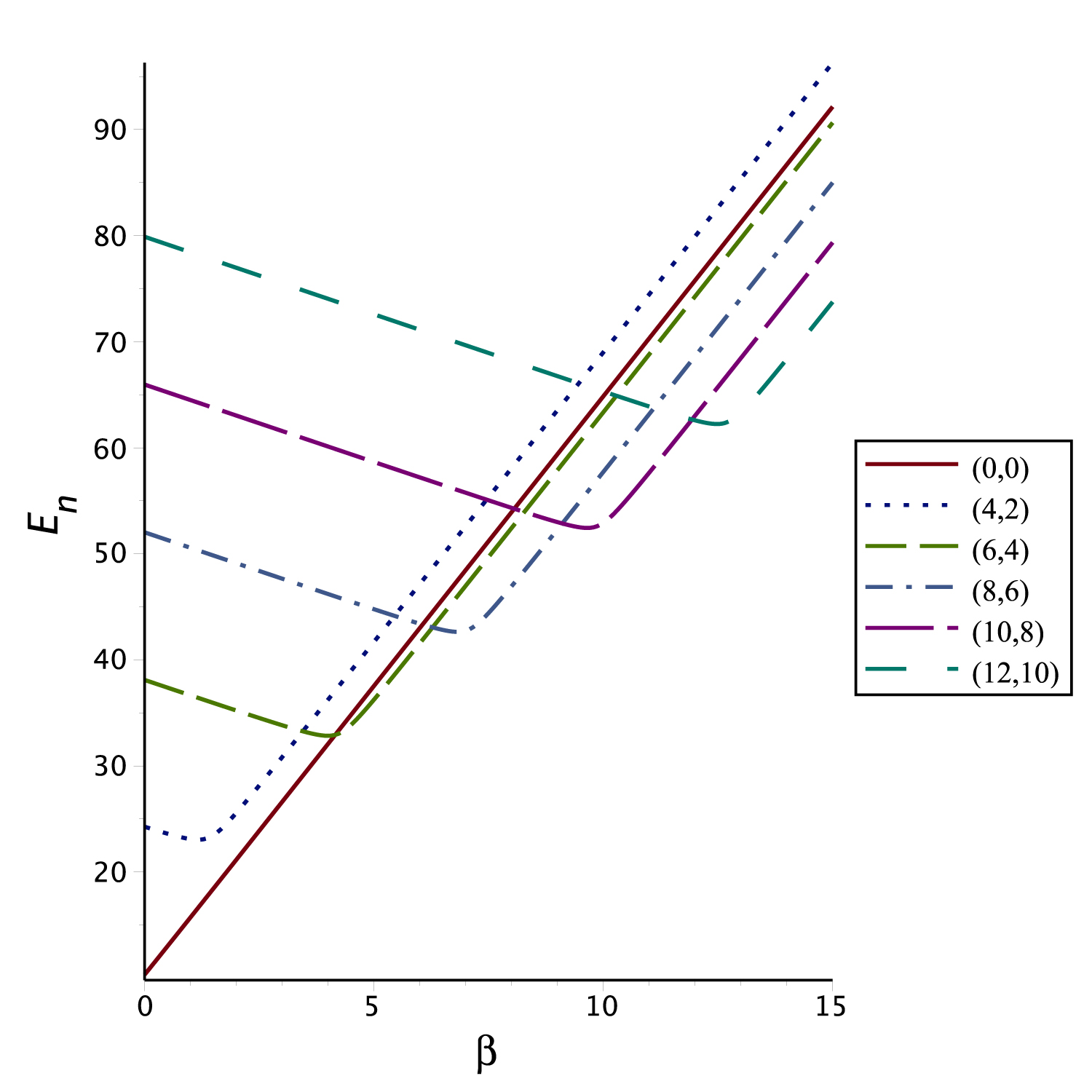
Figure 1: Energy levels $\left(n_{\rho}.m\right)$ crossings of (27) for different values $\beta$ in (19).

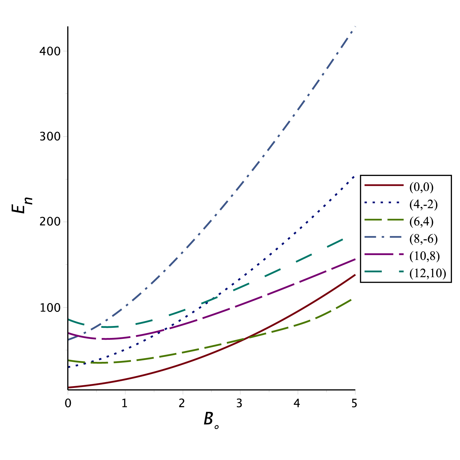
Figure 2: Energy levels $\left(n_{\rho}.m\right)$ crossings of (27) for different values of the magnetic field strength $B_{\circ}$ in (19).

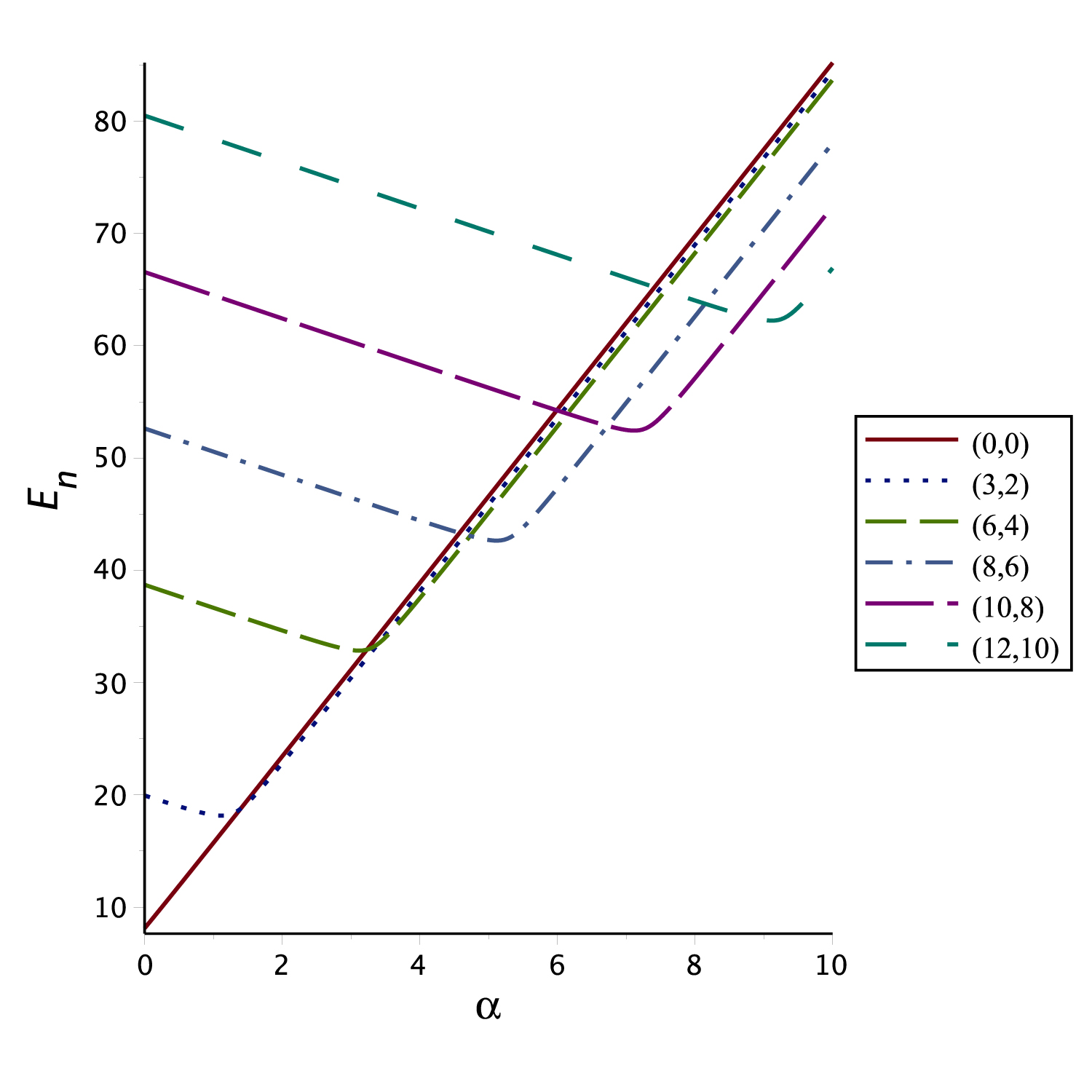
Figure 3: Energy levels $\left(n_{\rho}.m\right)$ crossings of (27) for different Aharonov-Bohm quantum number $\alpha$.

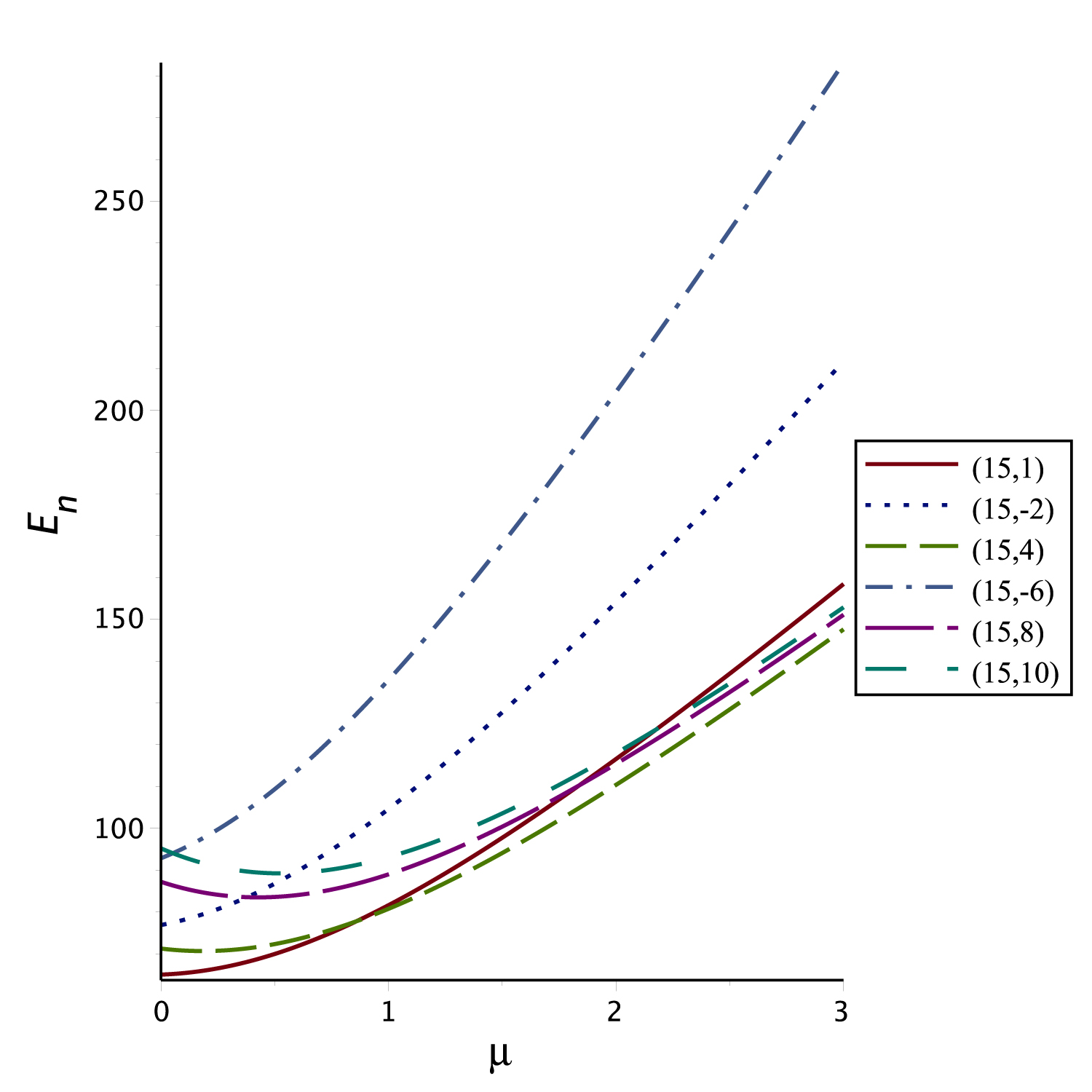
Figure 4: Energy levels $\left(n_{\rho}.m\right)$ crossings of (27) for different values of the magnetic field parameter $\mu$ in (19).

In Fig.s 1-4 we plot the energy levels (labeled as $\left(n_{\rho}.m\right)$) in (27) for different values of the parameters involved. The quantum numbers of a given state $\left(n_{\rho}.m\right)$ are chosen at random so that the phenomenon of energy levels crossings is made clear. The energy levels crossing points suggest that there could be more than one quantum state sharing the same energy at each crossing point. This would in turn indicate occasional degeneracies at some specific parametric settings.

III.2 An almost quasi-free PDM-charged particle of $g\left(\rho\right)=\eta/\rho^{2}$

An almost quasi-free PDM-charged particle with $g\left(\rho\right)=\eta/\rho^{2}$ (i.e., $f\left(\rho\right)=1/\rho^{2}$ and $\delta=0$ in (22)) moving under the influence of only the vector potential (8) would result in presenting (20) as

$$\left\{-\frac{d^{2}}{d\rho^{2}}+\frac{\acute{\ell}^{2}-1/4}{\rho^{2}}-\frac{\acute{\beta}}{\rho}\right\}U\left(\rho\right)=\tilde{E}\,U\left(\rho\right),$$ (29)

where,

$$\acute{\beta}=2e\tilde{m}B_{\circ}\mu-e^{2}B_{\circ}^{2}\mu\beta,$$ (30)

and

$$\acute{\ell}^{2}=\tilde{m}^{2}+\frac{1}{4}-e\tilde{m}B_{\circ}\beta+\frac{e^{2}B_{\circ}^{2}\beta^{2}}{4}-\eta E\Longleftrightarrow\left|\acute{\ell}\right|=\sqrt{\left(\tilde{m}-\frac{eB_{\circ}\beta}{2}\right)^{2}+\frac{1}{4}-\eta E}.$$ (31)

We have again a similar two-dimensional radial Schrödinger equation of Coulombic nature. One may, in a straightforward manner, show that it admits the exact eigenvalues

$$E_{n_{\rho},m,\alpha}=\frac{1}{\eta}\left[\left(m-\alpha-\frac{eB_{\circ}\beta}{2}\right)^{2}+\frac{1}{4}-\left(\frac{2e\left(m-\alpha\right)B_{\circ}\mu-e^{2}B_{\circ}^{2}\mu\beta}{2\sqrt{k_{z}^{2}+e^{2}B_{\circ}^{2}\mu^{2}}}-n_{\rho}-\frac{1}{2}\right)^{2}\right],$$ (32)

and exact radial wavefunctions

$$R_{n_{\rho},m,\alpha}\left(\rho\right)=\mathcal{N}\rho^{-1+\left|\acute{\ell}\right|}\exp\left(-\sqrt{k_{z}^{2}+e^{2}B_{\circ}^{2}\mu^{2}}\rho\right)L_{n_{\rho}}^{2\left|\acute{\ell}\right|}\left(2\sqrt{k_{z}^{2}+e^{2}B_{\circ}^{2}\mu^{2}}\rho\right)$$ (33)

In the Fig.s 5-8 we plot the energy levels $\left(n_{\rho}.m\right)$ in (32) for different values of the parameters involved. The the quantum states $\left(n_{\rho}.m\right)$ are chosen at random so that the phenomenon of energy levels crossings is made clear. One observes multiple energy levels crossings for each quantum state reported here. This would in turn indicate occasional degeneracies at some specific parametric settings.

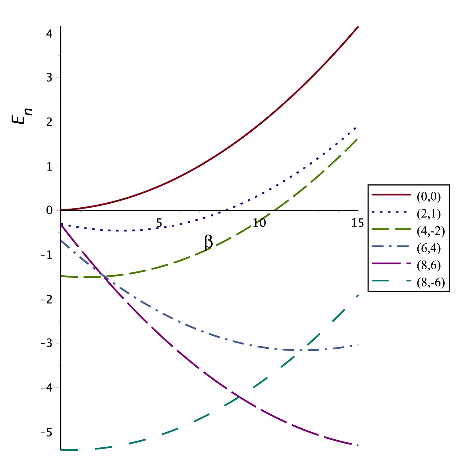
Figure 5: Energy levels $\left(n_{\rho}.m\right)$ crossings of (32) for different values of the parameter $\beta$ in (19).

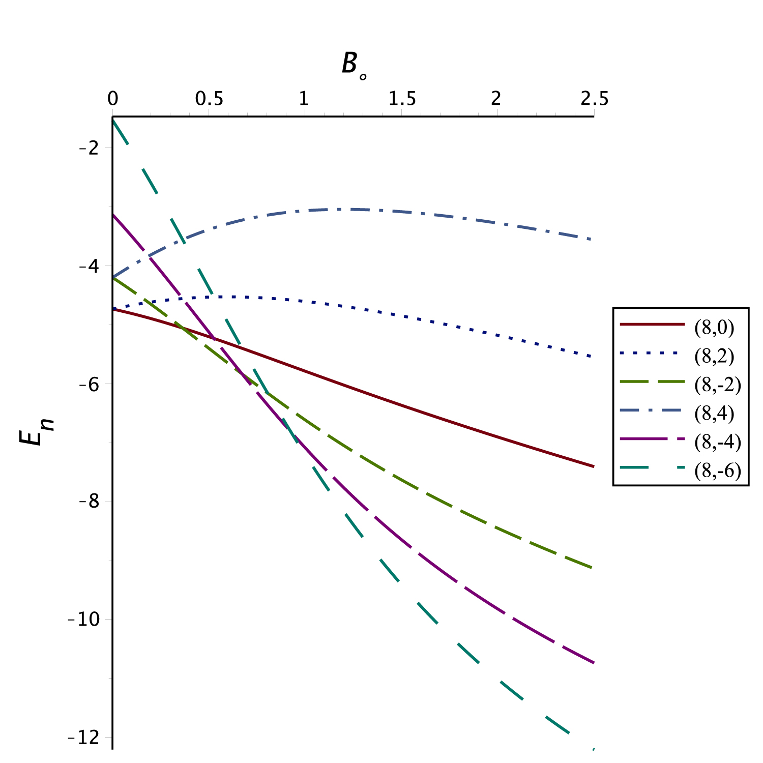
Figure 6: Energy levels $\left(n_{\rho}.m\right)$ crossings of (32) for different values of the magnetic field strength $B_{\circ}$ in (19).

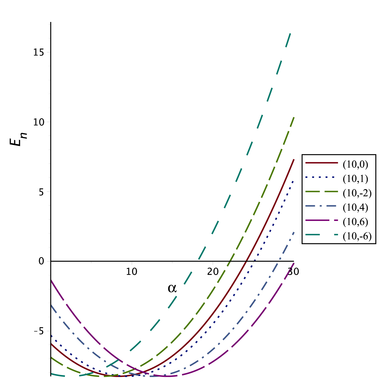
Figure 7: Energy levels $\left(n_{\rho}.m\right)$ crossings of (32) for different values of Aharonov-Bohm quantum number$\alpha$.

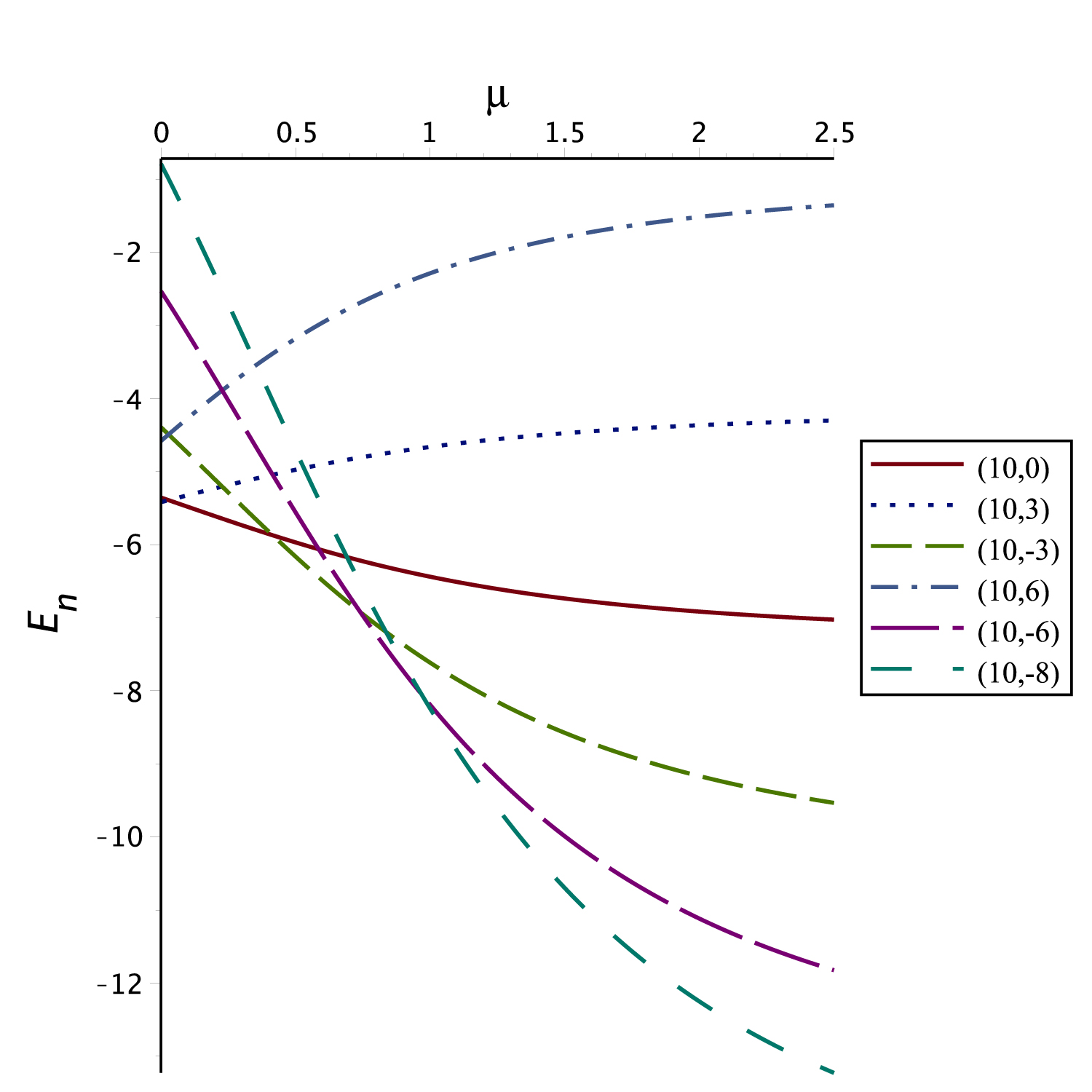
Figure 8: Energy levels $\left(n_{\rho}.m\right)$ crossings of (32) for different values of the magnetic field parameter $\mu$ in (19).

IV PDM-charged particles in PD-magnetic and Aharonov-Bohm flux fields: Nikiforov-Uvarov exact solvability

In this section, we shall be interested in a PDM-charged particle endowed with a Yukawa-type mass function

$$g\left(\rho\right)=\eta\left(\frac{\exp\left(-\delta\rho\right)}{\rho}\right)$$ (34)

(i.e., $f\left(\rho\right)=1/\rho$ and $\delta\neq 0$) moving in the vector potential (8) that yields the PD-magnetic field in (19). Moreover, we would like to subject this PDM-charged particle to radial confining potential of the form

$$V\left(\rho\right)=-\frac{V_{\circ}\exp\left(-\delta\rho\right)}{\rho}-\frac{V_{{}_{1}}}{\rho}+\frac{V_{{}_{2}}}{\rho^{2}},$$ (35)

which indulges within, a Yukawa-type (i.e., the first term) plus a Kratzer-type (the last two terms) potentials. A confinement potential type that is commonly used in the spectroscopy of the diatomic molecules, where the Greene-Aldrich approximation

$$\frac{1}{\rho}\simeq\frac{\delta}{1-\exp\left(-\delta\rho\right)}\Longleftrightarrow\frac{1}{\rho^{2}}\simeq\frac{\delta^{2}}{\left[1-\exp\left(-\delta\rho\right)\right]^{2}}$$ (36)

is valid for $\rho\ll 1$. Hence, equation (20) reads

$$\left\{-\frac{d^{2}}{d\rho^{2}}+\frac{a_{{}_{1}}}{\rho^{2}}+\frac{a_{{}_{2}}}{\rho}-a_{{}_{3}}\left(\frac{\exp\left(-\delta\rho\right)}{\rho}\right)+a_{{}_{4}}\right\}U\left(\rho\right)=0,$$ (37)

where

$$\begin{tabular}[]{cc}$a_{{}_{1}}=\tilde{m}^{2}-3/16-e\tilde{m}B_{\circ}\beta+e^{2}B_{\circ}^{2}\beta^{2}/4+V_{{}_{2}}\vskip 6.0pt plus 2.0pt minus 2.0pt,$&$a_{{}_{2}}=e^{2}B_{\circ}^{2}\mu\beta-2e\tilde{m}B_{\circ}\mu+3\delta/8-V_{{}_{1}}\vskip 6.0pt plus 2.0pt minus 2.0pt$\\ $a_{{}_{3}}=V_{\circ}+\eta\,E\vskip 6.0pt plus 2.0pt minus 2.0pt$&$a_{{}_{4}}=k_{z}^{2}+e^{2}B_{\circ}^{2}\mu^{2}+\delta^{2}/16\vskip 6.0pt plus 2.0pt minus 2.0pt$\end{tabular}.$$ (38)

Next, the use of Greene-Aldrich approximation (36) in (37) would allow us to rewrite it as

$$\left\{-\frac{d^{2}}{d\rho^{2}}+\frac{a_{{}_{1}}\delta^{2}}{\left[1-\exp\left(-\delta\rho\right)\right]^{2}}+\frac{a_{{}_{2}}\delta}{1-\exp\left(-\delta\rho\right)}-a_{{}_{3}}\left(\frac{\delta\exp\left(-\delta\rho\right)}{1-\exp\left(-\delta\rho\right)}\right)+a_{{}_{4}}\right\}U\left(\rho\right)=0.$$ (39)

Let us now use the substitution $\xi=\exp\left(-\delta\rho\right)$ and convert this equation into a Nikiforov-Uvarov type (see e.g. 39 ; 40 ; 41 ) to obtain

$$\left\{\frac{d^{2}}{d\xi^{2}}+\frac{\left(1-\xi\right)}{\xi\left(1-\xi\right)}\frac{d}{d\xi}+\frac{1}{\left[\xi\left(1-\xi\right)\right]^{2}}\left[-\left(\tilde{a}_{{}_{1}}-\tilde{a}_{{}_{2}}+\tilde{a}_{{}_{4}}\right)+\left(-\tilde{a}_{{}_{2}}+\tilde{a}_{{}_{3}}+2\tilde{a}_{{}_{4}}\right)\,\xi-\left(\tilde{a}_{{}_{3}}+\tilde{a}_{{}_{4}}\right)\,\xi^{2}\vskip 6.0pt plus 2.0pt minus 2.0pt\right]\right\}U\left(\xi\right)=0$$ (40)

where

$$\tilde{a}_{{}_{1}}=a_{{}_{1}}\text{ , }\tilde{a}_{{}_{2}}=-a_{{}_{2}}/\delta\text{ , }\tilde{a}_{{}_{3}}=a_{{}_{3}}/\delta\text{ , }\tilde{a}_{{}_{4}}=a_{{}_{4}}/\delta^{2}.$$ (41)

We may, therefore, express this equation in the Nikiforov-Uvarov form

$$U^{\prime\prime}\left(\xi\right)+\frac{\tilde{\tau}\left(\xi\right)}{\sigma\left(\xi\right)}U^{\prime}\left(\xi\right)+\frac{\tilde{\sigma}\left(\xi\right)}{\sigma\left(\xi\right)^{2}}U\left(\xi\right)=0,$$ (42)

where

$$\begin{tabular}[]{l}$\tilde{\tau}\left(\xi\right)\vskip 6.0pt plus 2.0pt minus 2.0pt=1-\xi$ , \ \ \ $\sigma\left(\xi\right)=\xi\left(1-\xi\right)$\\ $\tilde{\sigma}\left(\xi\right)=-\left(\tilde{a}_{{}_{1}}-\tilde{a}_{{}_{2}}+\tilde{a}_{{}_{4}}\right)+\left(-\tilde{a}_{{}_{2}}+\tilde{a}_{{}_{3}}+2\tilde{a}_{{}_{4}}\right)\,\xi-\left(\tilde{a}_{{}_{3}}+\tilde{a}_{{}_{4}}\right)\,\xi^{2}\vskip 6.0pt plus 2.0pt minus 2.0pt$\end{tabular}.$$ (43)

Which obviously satisfies the requirements of NU-method, where $\sigma\left(\xi\right)$, $\tilde{\sigma}\left(\xi\right)$ are polynomials of at most second degree, and $\tilde{\tau}\left(\xi\right)$ is at most a first degree polynomial. Although the NU-method is well known, we would like to recycle it in an optimal way that makes the current paper self-contained and clear. We do so in the Appendix.

Following NU-method procedure of the Appendix (namely, equations (A.1) to (A.20)), with $\tilde{a}_{{}_{3}}=\left(\eta E+V_{\circ}\right)/\delta$ in (41) and (38), we obtain

$$\tilde{a}_{{}_{3}}=\left(n_{\rho}^{2}+n_{\rho}+1/2\right)+\left(2n_{\rho}+1\right)\epsilon_{1}+\epsilon_{2}$$ (44)

where $\epsilon_{1}$ and $\epsilon_{2}$ are given through the relations $\epsilon_{1}=\tilde{\epsilon}_{1}/\delta$ and $\epsilon_{2}=\tilde{\epsilon}_{2}/\delta$ so that

$$\tilde{\epsilon}_{1} = \left[\delta^{2}\left(\tilde{m}-\frac{eB_{\circ}\beta}{2}\right)^{2}+\delta^{2}V_{2}+\frac{\delta^{2}}{4}-2eB_{\circ}\mu\left(\tilde{m}-\frac{eB_{\circ}\beta}{2}\right)\delta-\delta V_{1}+e^{2}B_{\circ}^{2}\mu^{2}+k_{z}^{2}\right]^{1/2}\vskip 6.0pt plus 2.0pt minus 2.0pt$$ (45)

$$+\delta\,\left[\left(\tilde{m}-\frac{eB_{\circ}\beta}{2}\right)^{2}+V_{2}+\frac{1}{16}\right]^{1/2},$$

and

$$\tilde{\epsilon}_{2} = 2\left\{\left[\delta^{2}\left(\tilde{m}-\frac{eB_{\circ}\beta}{2}\right)^{2}+\delta^{2}V_{2}+\frac{\delta^{2}}{4}-2eB_{\circ}\mu\left(\tilde{m}-\frac{eB_{\circ}\beta}{2}\right)\delta-\delta V_{1}+e^{2}B_{\circ}^{2}\mu^{2}+k_{z}^{2}\right]\right.$$ (46)

$$\times\left.\left[\left(\tilde{m}-\frac{eB_{\circ}\beta}{2}\right)^{2}+V_{2}+\frac{1}{16}\right]\right\}^{1/2}\vskip 6.0pt plus 2.0pt minus 2.0pt+2\left[\delta\left(\tilde{m}-\frac{eB_{\circ}\beta}{2}\right)^{2}+\delta V_{2}-eB_{\circ}\mu\left(\tilde{m}-\frac{eB_{\circ}\beta}{2}\right)\right]-V_{1}.$$

This would eventually imply

$$E_{n_{\rho},m,\alpha}=\frac{1}{\eta}\left\{\left(n_{\rho}^{2}+n_{\rho}+1/2\right)\delta+\left(2n_{\rho}+1\right)\tilde{\epsilon}_{1}+\tilde{\epsilon}_{2}-V_{\circ}\right\}$$ (47)

One should notice that the result in (47) recovers that of the almost quasi-free PDM-charged particle in (27) by setting $\delta=0$ and $V_{\circ}=V_{1}=V_{2}=0$ in (34) and (35). This should be the typical tendency (as well as a double check) of the exact analytical solution of the more general problem discussed here, of course. Moreover, our radial wave functions are given by (15), (A.1), and (A.23) to yield

$$R_{n_{\rho},m,\alpha}\left(\rho\right)=\mathcal{N}_{n_{\rho}}\mathcal{\,\rho}^{{}^{-\left(1-\upsilon\right)/2}}\exp\left(-\delta\rho\left(1+\kappa\right)/2\right)P_{n_{\rho}}^{\left(\kappa,\upsilon\right)}\left(1-2e^{-\delta\rho}\right)\vskip 6.0pt plus 2.0pt minus 2.0pt$$ (48)

where $\mathcal{N}_{n_{\rho}}$ is the corresponding normalization constant. Yet, this result would collapse into that of the almost quasi-free PDM-charged particle in (28) for $\delta=0$ and $V_{\circ}=V_{1}=V_{2}=0$ in (34) and (35). In Fig. 9 we plot the energies of (47) against the PDM parameter $\delta$ of (34). We observe a direct effect of the PDM on the energy levels crossings indicating again occasional degeneracies.

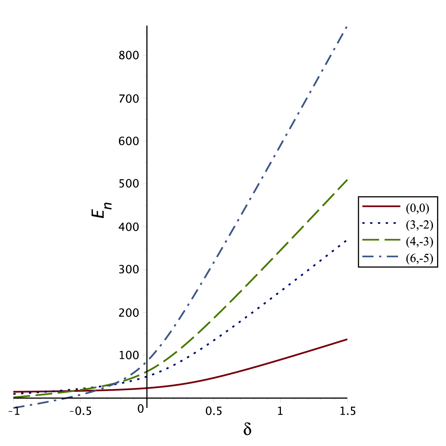
Figure 9: Energy levels $\left(n_{\rho}.m\right)$ crossings of (47) for different values $\delta$ in (34).

V Concluding Remarks

We have considered, using cylindrical coordinates under azimuthal symmetrization, some PDM-charged particles in PD-magnetic and Aharonov-Bohm flux fields. Two almost-quasi-free PDM-charged particles (i.e., no conventional confinement potential, $V\left(\overrightarrow{r}\right)=0$, and the only interaction is provided by the PDM-minimal coupling along with the position-dependent mass) with $g\left(\rho\right)=\eta/\rho$ and $g\left(\rho\right)=\eta/\rho^{2}$ turned out to imply exactly solvable radial Schrödinger equations of a Coulombic nature (documented in (27) and (28) for $g\left(\rho\right)=\eta/\rho$ and (32) and (33) for $g\left(\rho\right)=\eta/\rho^{2}$). Their exact solutions are inferred, in a straightforward manner, from the textbook solutions. Moreover, a more general Yukawa-type PDM-charged particle with $g\left(\rho\right)=\eta\,\exp\left(-\delta\rho\right)/\rho$ moving not only in the PD-magnetic and Aharonov-Bohm flux fields but also in the vicinity of a Yukawa plus a Kratzer type confinement potential field $V\left(\rho\right)=-V_{\circ}\exp\left(-\delta\rho\right)/\rho-V_{{}_{1}}/\rho+V_{{}_{2}}/\rho^{2}$ is considered. For this case, we have used the NU-method to obtain exact analytical eigenvalues and eigenfunctions (reported in (47) and (48), respectively). Our observations are in order.

The energy levels crossings are observed eminent for the two almost-quasi-free PDM-charged particles in (27) ( for $g\left(\rho\right)=\eta/\rho$) and (32) (for $g\left(\rho\right)=\eta/\rho^{2}$). We have, therefore, reported Figures 1-8 so that this phenomenon of levels crossings is made clear. The quantum states involved in the plots are labeled as $\left(n_{\rho}.m\right)$ and the quantum numbers $n_{\rho}$ and $m$ are chosen at random. Such energy levels crossing points suggest that there could be more than one quantum state sharing the same energy at each crossing point. For example, Fig.1 shows the effect of the parameter $\beta$ of the magnetic field generating function (19) on the energy levels of (27). Hereby, we observe that the state labeled $\left(12,10\right)$ crosses with $\left(4,2\right)$, $\left(6,4\right)$, $\left(8,6\right)$, $\left(0,1\right)$, $\left(10,8\right)$. This would indicate that the state $\left(12,10\right)$ share the same energy with $\left(4,2\right)$, $\left(6,4\right)$, $\left(8,6\right)$, $\left(0,1\right)$, $\left(10,8\right)$ at the crossing points. Similar scenarios of energy levels crossings are also observed in Fig.s 2-8. Where, Fig.s 1 and 5 show the effect of $\beta$, Fig.s 2 and 6 show the effect of the magnetic field strength $B_{\circ}$ of (19), Fig.s 3 and 7 show the effect the Aharonov-Bohm quantum number $\alpha$, and Fig.s 4 and 8 show the effect the magnetic field parameter $\mu$ on the energy levels of (27) and (32), respectively. Such energy levels crossings may very well be classified as ”occasional degeneracies” that have erupted as a result of PDM setting. Energy levels crossings are also observed feasible in (47) for the Yukawa-type PDM-charged particles of (34) confined in the Yukawa-plus-Kratzer potential (35). This is documented in Fig. 9, where a direct influence of the PDM-parameter $\delta$ of (34) on the energy levels crossings is observed.

On the position-dependent settings side, we have chosen, in (19), to work with a PD-magnetic field $\overrightarrow{B}=\left(B_{\circ}\mu/\rho\,\right)\widehat{z}$ (i.e., $\sigma=1$ in (18)). In so doing, we sought simplicity and physical eligibility in order to make the current methodical proposal instructive  and clear. Of course, one may wish to work with other values for $\sigma$ in (18), as yet another form for the PD-magnetic field, and follow the same procedure to find the eigenvalues and eigenfunctions. Moreover, our choices for the PDM-functions in (23), (29), and (34) are manifested meanly by  the convenience of the current study.

Finally, we have asserted that a deformation on the coordinate system may very well render the mass position-dependent 11 ; 31 (i.e., the mass becomes metaphorically speaking position-dependent). One may, therefore, use the eigen energies to calculate the partition functions and discuss some thermodynamical properties (see, e.g., 41 ; 44 ; 45 ) of such PDM systems in PD-magnetic and Aharonov Bohm fields and, perhaps, in diatomic confining potentials like the Tietz oscillator, Rosen-Morse, Manning-Rosen, etc.

VI Appendix: Nikiforov-Uvarov method

In this section, we recycle it in an optimal way that makes the current paper self-contained and clear. We, therefore, closely follow Badalov 39 (where instructive and informative details on NU-method are available). As such, a substitution of the form

$$U\left(\xi\right)=\phi\left(\xi\right)\chi\left(\xi\right)$$ (A.1)

in (42) would lead to a hypergeometric-type equation

$$\sigma\left(\xi\right)\chi^{\prime\prime}\left(\xi\right)+\tau\left(\xi\right)\chi^{\prime}\left(\xi\right)+\lambda\chi\left(\xi\right)=0$$ (A.2)

where its solutions $\chi_{n}\left(\xi\right)$ satisfy the Rodrigues relation

$$\chi_{n}\left(\xi\right)=\frac{A_{n}}{\omega\left(\xi\right)}\frac{d^{n}}{d\xi^{n}}\left(\sigma^{n}\left(\xi\right)\omega\left(\xi\right)\right)\text{ };\text{ \ }n=0,1,2,\cdots$$ (A.3)

and the weight function $\omega\left(\xi\right)$ satisfies the condition

$$\frac{d}{d\xi}\left(\sigma\left(\xi\right)\omega\left(\xi\right)\right)=\tau\left(\xi\right)\omega\left(\xi\right).$$ (A.4)

Here, we have used

$$\pi\left(\xi\right)=\sigma\left(\xi\right)\frac{\phi^{\prime}\left(\xi\right)}{\phi\left(\xi\right)}\text{, }\tau\left(\xi\right)=\tilde{\tau}\left(\xi\right)+2\pi\left(\xi\right)\text{ , \ }\lambda=\frac{\phi^{\prime\prime}\left(\xi\right)}{\phi\left(\xi\right)}\sigma\left(\xi\right)+\frac{\tilde{\tau}\left(\xi\right)}{\sigma\left(\xi\right)}\pi\left(\xi\right)+\frac{\tilde{\sigma}\left(\xi\right)}{\sigma\left(\xi\right)}$$ (A.5)

with the condition $\tau^{\prime}\left(\xi\right)<0$ is imposed on the weight function $\omega\left(\xi\right)$. The parameter $\lambda$ required for this method is also defined as

$$\lambda=k+\pi^{\prime}\left(\xi\right).$$ (A.6)

Hence, (A.5) and (A.6) yield

$$\pi\left(\xi\right)=\frac{\sigma^{\prime}\left(\xi\right)-\tilde{\tau}\left(\xi\right)}{2}\pm\sqrt{\frac{\left(\sigma^{\prime}\left(\xi\right)-\tilde{\tau}\left(\xi\right)\right)^{2}}{4}+k\sigma\left(\xi\right)-\tilde{\sigma}\left(\xi\right)}.$$ (A.7)

To find the value of $k$ in (A.7), one should be able to write the expression under the square root in the form of a quadratic equation (i.e., square of a polynomial of first degree). That is, the expression under the square root should look like $A\xi^{2}+B\xi+C\Longleftrightarrow\left(\sqrt{A}\xi\pm\sqrt{C}\right)^{2}$ so that $B=\pm 2\sqrt{AC}$ is a condition imposed on the adjustable parameter $k$. Moreover, the eigenvalues of the hypergeometric equation (A.2) are given by

$$\lambda=\lambda_{n}=-n\tau^{\prime}\left(\xi\right)-\frac{n\left(n-1\right)}{2}\sigma^{\prime\prime}\left(\xi\right)\text{ };\text{ }n=0,1,2,\cdots$$ (A.8)

Consequently, our $\pi\left(\xi\right)$ is given by

$$\pi\left(\xi\right)=-\frac{\xi}{2}\pm\sqrt{A\xi^{2}+B\xi+C}=-\frac{\xi}{2}\pm\left(\sqrt{A}\xi\pm\sqrt{C}\right);\,B=\pm 2\sqrt{AC},$$ (A.9)

where

$$A=1/4-k+\tilde{a}_{{}_{3}}+\tilde{a}_{{}_{4}},$$

(A.10)

At this point, we recollect that

$$\tau\left(\xi\right)=\tilde{\tau}\left(\xi\right)+2\pi\left(\xi\right)\Longleftrightarrow\tau^{\prime}\left(\xi\right)=-2\pm 2\sqrt{A},$$ (A.11)

which suggests that the condition $\tau^{\prime}\left(\xi\right)<0$ is satisfied if and only if

$$\tau^{\prime}\left(\xi\right)=-2-2\sqrt{A}\Longleftrightarrow\pi\left(\xi\right)=\pi_{{}_{-}}\left(\xi\right)=-\frac{\xi}{2}-\left(\sqrt{A}\xi\pm\sqrt{C}\right)\Leftrightarrow\tau\left(\xi\right)=\tilde{\tau}\left(\xi\right)+2\pi_{{}_{-}}\left(\xi\right),$$ (A.12)

provided that $A>0$ in (A.10) otherwise unphysical imaginary energy eigenvalues are obtained by (A.8). Moreover, the relation $B=\pm 2\sqrt{AC}\Longleftrightarrow B^{2}=4AC$ in (A.9) would imply that

$$k=k_{{}_{\pm}}=-\left(2\tilde{a}_{{}_{1}}-\tilde{a}_{{}_{2}}-\tilde{a}_{{}_{3}}\right)\pm\sqrt{\left(\tilde{a}_{{}_{1}}-\tilde{a}_{{}_{2}}+\tilde{a}_{{}_{4}}\right)\left(4\tilde{a}_{{}_{1}}+1\right)}.$$

Consequently, the condition that $A=1/4-k+\tilde{a}_{{}_{3}}+\tilde{a}_{{}_{4}}>0$ of (A.10) would necessarily imply that

$$k=k_{{}_{-}}=-\left(2\tilde{a}_{{}_{1}}-\tilde{a}_{{}_{2}}-\tilde{a}_{{}_{3}}\right)-\sqrt{\left(\tilde{a}_{{}_{1}}-\tilde{a}_{{}_{2}}+\tilde{a}_{{}_{4}}\right)\left(4\tilde{a}_{{}_{1}}+1\right)}.$$ (A.13)

Now we go back to our $\pi\left(\xi\right)$ of (A.9), along with (A.10) and $k=k_{{}_{-}}$ in (A.13), and cast it as

$$\pi\left(\xi\right)=\pi_{{}_{-}}\left(\xi\right)=-\frac{\xi}{2}-\sqrt{A_{{}_{-}}\xi^{2}+B_{{}_{-}}\xi+C},$$ (A.14)

where, in this case, equation (A.10) suggests that

$$A=A_{{}_{-}}=\frac{1}{4}-k_{{}_{-}}+\tilde{a}_{{}_{3}}+\tilde{a}_{{}_{4}}=\left(\frac{4\tilde{a}_{{}_{1}}+1}{4}\right)+\left(\tilde{a}_{{}_{1}}-\tilde{a}_{{}_{2}}+\tilde{a}_{{}_{4}}\right)+\sqrt{\left(\tilde{a}_{{}_{1}}-\tilde{a}_{{}_{2}}+\tilde{a}_{{}_{4}}\right)\left(4\tilde{a}_{{}_{1}}+1\right)},$$ (A.15)

and

$$B=B_{{}_{-}}=k_{{}_{-}}+\tilde{a}_{{}_{2}}-\tilde{a}_{{}_{3}}-2\tilde{a}_{{}_{4}}=-2\sqrt{\tilde{a}_{{}_{1}}-\tilde{a}_{{}_{2}}+\tilde{a}_{{}_{4}}}\left(\sqrt{\tilde{a}_{{}_{1}}-\tilde{a}_{{}_{2}}+\tilde{a}_{{}_{4}}}+\sqrt{\frac{4\tilde{a}_{{}_{1}}+1}{4}}\right).$$ (A.16)

Next, a straightforward rearrangement of the terms in (A.14) immediately yields

$$\pi_{{}_{-}}\left(\xi\right)=-\frac{\xi}{2}-\left[\left(\sqrt{\tilde{a}_{{}_{1}}-\tilde{a}_{{}_{2}}+\tilde{a}_{{}_{4}}}+\sqrt{\frac{4\tilde{a}_{{}_{1}}+1}{4}}\right)\xi-\sqrt{\tilde{a}_{{}_{1}}-\tilde{a}_{{}_{2}}+\tilde{a}_{{}_{4}}}\right]$$ (A.17)

This would, in turn, imply that the condition

$$\tau^{\prime}\left(\xi\right)=-2-2\left(\sqrt{\tilde{a}_{{}_{1}}-\tilde{a}_{{}_{2}}+\tilde{a}_{{}_{4}}}+\sqrt{\frac{4\tilde{a}_{{}_{1}}+1}{4}}\right)<0.$$ (A.18)

is satisfied. We are now at a point where we can calculate the eigenvalues working with (A.6)

$$\lambda=k_{{}_{-}}+\pi_{{}_{-}}^{\prime}\left(\xi\right)=-\left(2\tilde{a}_{{}_{1}}-\tilde{a}_{{}_{2}}-\tilde{a}_{{}_{3}}\right)-\sqrt{\left(\tilde{a}_{{}_{1}}-\tilde{a}_{{}_{2}}+\tilde{a}_{{}_{4}}\right)\left(4\tilde{a}_{{}_{1}}+1\right)}-\frac{1}{2}-\sqrt{\tilde{a}_{{}_{1}}-\tilde{a}_{{}_{2}}+\tilde{a}_{{}_{4}}}-\sqrt{\frac{4\tilde{a}_{{}_{1}}+1}{4}}$$ (A.19)

and (A.8)

$$\lambda=\lambda_{n}=-n\tau^{\prime}\left(\xi\right)-\frac{n\left(n-1\right)}{2}\sigma^{\prime\prime}\left(\xi\right)=n\left[2+2\left(\sqrt{\tilde{a}_{{}_{1}}-\tilde{a}_{{}_{2}}+\tilde{a}_{{}_{4}}}+\sqrt{\frac{4\tilde{a}_{{}_{1}}+1}{4}}\right)\right]+n\left(n-1\right)$$ ((A.20))

On the other hand, the eigenfunctions $U\left(\xi\right)=\phi\left(\xi\right)\chi\left(\xi\right)$ are obtained in a straightforward manner. That is,

$$\frac{\phi^{\prime}\left(\xi\right)}{\phi\left(\xi\right)}=\frac{\pi_{{}_{-}}\left(\xi\right)}{\sigma\left(\xi\right)}\Longleftrightarrow\phi\left(\xi\right)=\xi^{\sqrt{\tilde{a}_{{}_{1}}-\tilde{a}_{{}_{2}}+\tilde{a}_{{}_{4}}}}\left(1-\xi\right)^{\frac{1}{2}+\frac{1}{2}\sqrt{4\tilde{a}_{{}_{1}}+1}},\vskip 6.0pt plus 2.0pt minus 2.0pt$$ (A.21)

and the weight function $\omega\left(\xi\right)$ is calculated through (A.4) to obtain

$$\frac{\omega^{\prime}\left(\xi\right)}{\omega\left(\xi\right)}=\frac{\tau\left(\xi\right)-\sigma^{\prime}\left(\xi\right)}{\sigma\left(\xi\right)}\Longleftrightarrow\omega\left(\xi\right)=\xi^{2\sqrt{\tilde{a}_{{}_{1}}-\tilde{a}_{{}_{2}}+\tilde{a}_{{}_{4}}}}\left(1-\xi\right)^{\sqrt{4\tilde{a}_{{}_{1}}+1}}.$$ (A.22)

Consequently, the Rodrigues relation (A.3), with $\kappa=2\left(\sqrt{\tilde{a}_{{}_{1}}-\tilde{a}_{{}_{2}}+\tilde{a}_{{}_{4}}}\right)$ and $\upsilon=\sqrt{4\tilde{a}_{{}_{1}}+1}$, implies

$$\chi_{n_{\rho}}\left(\xi\right)=A_{n_{\rho}}\,\xi^{-\kappa}\left(1-\xi\right)^{-\upsilon}\frac{d^{n_{\rho}}}{d\xi^{n_{\rho}}}\left[\xi^{n_{\rho}+\kappa}\left(1-\xi\right)^{n_{\rho}+\upsilon}\right]=\tilde{A}_{n_{\rho}}\,P_{n_{\rho}}^{\left(\kappa,\upsilon\right)}\left(1-2\xi\right)\,;\text{ \ }\xi\in\left[0,1\right]\vskip 6.0pt plus 2.0pt minus 2.0pt$$ (A.23)

where $P_{n}^{\left(\kappa,\upsilon\right)}\left(1-2\xi\right)$ are the Jacobi polynomials satisfying the Rodrigues’ formula

$$P_{n}^{\left(\alpha,\beta\right)}\left(x\right)=\frac{\left(-1\right)^{n}}{2^{n}n!}\left(1-x\right)^{-\alpha}\left(1+x\right)^{-\beta}\frac{d^{n}}{dx^{n}}\left[\left(1-x\right)^{n+\alpha}\left(1+x\right)^{n+\beta}\right]\,;\,x\in\left[-1,1\right].\vskip 6.0pt plus 2.0pt minus 2.0pt$$ (A.24)

Hereby, we have used $x=2\xi-1$ along with the polynomials symmetry relation

$$P_{n}^{\left(\alpha,\beta\right)}\left(x\right)=\left(-1\right)^{n}P_{n}^{\left(\beta,\alpha\right)}\left(-x\right)\Longleftrightarrow P_{n}^{\left(\upsilon,\kappa\right)}\left(2\xi-1\right)=\left(-1\right)^{n}P_{n}^{\left(\kappa,\upsilon\right)}\left(1-2\xi\right),$$ (A.25)

( with $\beta=\kappa$ and $\alpha=\upsilon$) to obtain (A.23).

References

- (1) A. Das, J. Frenkel, S. H. Pereira, J. C. Taylor, Quantum behavior of a charged particle in an axial magnetic field, Phys. Rev. A 70 (2004) 053408
- (2) I. Wayan Sudiarta, D. J. Wallace Geldart, Solving the Schrödinger equation for a charged particle in a magnetic field using the finite difference time domain method, Phys. Lett. A 372 (2008) 3145-3148.
- (3) H. Asnani, R. Mahajan, P. Pathak, V. A. Singh, Effective mass theory of two - dimensional quantum dot in the presence of a magnetic field, Pramana-J. Phys. 73 (2009) 573-580.
- (4) E. N. Bogachek, U. Landman, Edge states, Aharonov-Bohm oscillations, and thermodynamic and spectral properties in a two-dimensional electron gas with an antidot, Phys. Rev. B 52 (1995) 14067.
- (5) A. Cetin, A quantum pseudodot system with a two-dimensional pseudoharmonic potential, Phys. Lett. A 372 (2008) 3852.
- (6) S. M. Ikhdair, M. Hamzavi, A quantum pseudodot system with two-dimensional pseudoharmonic oscillator in external magnetic and Aharonov-Bohm fields, Physica B: Condensed Matter 407 (2012) 4198.
- (7) M. Eshghi, H. Mehraban, S. M. Ikhdair, Approximate energies and thermal properties of a position-dependent mass charged particle under external magnetic fields, Chin. Phys. B 26 (2017) 060302.
- (8) M.S. Atoyan, E. M. Kazaryan, H. A. Sarkisyan, Interband light absorption in parabolic quantum dot in the presence of electrical and magnetic fields, Physica E 31 (2006) 83.
- (9) O. Mustafa,The shifted-1/N-expansion method for two-dimensional hydrogenic donor states in an arbitrary magnetic field, J. Phys.:Condensed Matter 5 (1993) 1327.
- (10) O. Mustafa, S. C. Chhajlany, Ground-state energies of hydrogenic atoms in a uniform magnetic field of arbitrary strength, Phys. Rev. A 50 (1994) 2926.
- (11) O. Mustafa, Z. Algadhi, Position-dependent mass momentum operator and minimal coupling: point canonical transformation and isospectrality, Eur. Phys. J. Plus 134 (2019) 228.
- (12) O. von Roos, Position-dependent effective masses in semiconductor theory, Phys. Rev. B 27 (1983) 7547.
- (13) A. de Souza Dutra, C A S Almeida, Exact solvability of potentials with spatially dependent effective masses, Phys Lett. A 275 (2000) 25.
- (14) C. Tezcan, R. Sever, O. Yesiltas, A new approach to the exact solutions of the effective mass Schrödinger equation, Int. J. Theor. Phys, 47 (2008) 1713.
- (15) O. Mustafa, S. H. Mazharimousavi, Quantum particles trapped in a position-dependent mass barrier; a d-dimensional recipe, Phys. Lett. A 358 (2006) 259.
- (16) A. D. Alhaidari, Solutions of the nonrelativistic wave equation with position-dependent effective mass, Phys. Rev. A 66 (2002) 042116.
- (17) O. Mustafa, Energy-levels crossing and radial Dirac equation: supersymmetry and quasi-parity spectral signatures, Int. J. Theor. Phys. 47 (2008) 1300.
- (18) R. Bravo, M. S. Plyushchay, Position-dependent mass, finite-gap systems, and supersymmetry, Phys. Rev. D 93 (2016) 105023.
- (19) C. Quesne, V. M. Tkachuk, Deformed algebras, position-dependent effective masses and curved spaces: an exactly solvable Coulomb problem, J. Phys. A 37 (2004) 4267.
- (20) B. Bagchi, P. Gorain, C. Quesne and R. Roychoudhury, A general scheme for the effective-mass Schrodinger equation and the generation of the associated potentials, Mod. Phys. Lett. A 19 (2004) 2765.
- (21) Y. C. Ou, Z. Cao, Q. Shen, Energy eigenvalues for the systems with position-dependent effective mass, J. Phys. A: Math. Gen. 37 (2004) 4283-4288.
- (22) O. Mustafa, S. H. Mazharimousavi, Comment on ’Position-dependent effective mass Dirac equations with PT-symmetric and non-PT-symmetric potentials’, J. Phys. A: Math. Theor. 40 (2007) 863.
- (23) R. A. C. Correa, A. de Souza Dutra, J A de Oliveira, M.G. Garcia, A complete set of eigenstates for position-dependent massive particles in a Morse-like scenario, J. Math. Phys. 58 (2017) 012104
- (24) O. Mustafa, S. H. Mazharimousavi, Ordering ambiguity revisited via position dependent mass pseudo-momentum operators, Int. J. Theor. Phys. 46 (2007) 1786.
- (25) A. de Souza Dutra, Ordering ambiguity versus representation, J. Phys. A: Math. Gen. 39 (2006) 203.
- (26) G. T. Einevoll, P. C. Hemmer, J. Thomsen, Operator ordering in effective-mass theory for heterostructures. I. Comparison with exact results for superlattices, quantum wells, and localized potentials, Phys. Rev. B 42, (1990) 3485.
- (27) R. Koc, G. Sahinoglu, M. Koca, Scattering in abrupt heterostructures using a position dependent mass Hamiltonian, Eur. Phys. J.B 48 (2005) 583.
- (28) S. H. Mazharimousavi, O. Mustafa, Classical and quantum quasi-free position-dependent mass: Pöschl–Teller and ordering ambiguity, Phys. Scr. 87 (2013) 055008.
- (29) B. Bagchi, A. Banerjee, C. Quesne, V. M. Tkachuk, Deformed shape invariance and exactly solvable Hamiltonians with position-dependent effective mass, J. Phys. A: Math. Gen. 38 (2005) 2929.
- (30) S. G. Hua, D. Popov, O. C. Nieto, D. S. Hai, Shannon information entropies for position-dependent mass Schrödinger problem with a hyperbolic well, Chin. Phys. B 34 (2015) 100303.
- (31) O. Mustafa, Position-dependent mass Lagrangians: nonlocal transformations, Euler–Lagrange invariance and exact solvability, J. Phys. A; Math. Theor. 48 (2015) 225206.
- (32) B. G. da Costa, E. P. Borges, A position-dependent mass harmonic oscillator and deformed space, J. Math. Phys. 59 (2018) 042101.
- (33) O. Mustafa, Position-dependent-mass: cylindrical coordinates, separability, exact solvability and PT -symmetry, J. Phys. A: Math. Theor. 43 (2010) 385310.
- (34) O. Mustafa, Radial power-law position-dependent mass: cylindrical coordinates, separability and spectral signatures, J Phys A: Math. Theor. 44 (2011) 355303.
- (35) A . de Souza Dutra, J. A. de Oliveira, Two-dimensional position-dependent massive particles in the presence of magnetic fields, J. Phys. A: Math. Theor. 42, (2009) 025304.
- (36) O. Mustafa, Comment on ’Two-dimensional position-dependent massive particles in the presence of magnetic fields’, J. Phys. A: Math. Theor. 52 (2019) 148001.
- (37) Q. Yu, K. Guo, M. Hu, Z. Zhang, K. Li, D. Liu, Study on the optical rectification and second-harmonic generation with position-dependent mass in a quantum well, J. Phys. Chem. Solid. 119 (2018) 50.
- (38) E. Paspalakis, D. Stefanatos, Comment on “Study on the optical rectification and second-harmonic generation with position-dependent mass in a quantum well” [Journal of Physics and Chemistry of Solids, 119 (2018) 50–55], J. Phys. Chem. Solid. 126 (2019) 178.
- (39) V. H. Badalov, The bound state solutions of the D-dimensional Schrödinger equation for the Woods–Saxon potential, Int. J. Mod. Phys. E 25 (2016) 1650002.
- (40) S. M. Ikhdair, R. Sever, Relativistic and nonrelativistic bound states of the isotonic oscillator by Nikiforov-Uvarov method, J. Math. Phys. 52 (2011) 122108.
- (41) M. Eshghi, R. Sever, S. M. Ikhdair, Energy states of the Hulthen plus Coulomb-like potential with position-dependent mass function in external magnetic fields, Chin. Phys. B 27 (2018) 020301.
- (42) O. Mustafa, Z. Algadhi: arXiv:1907.11592 ”Position-dependent mass charged particles in magnetic and Aharonov-Bohm flux fields: separability, exact and conditionally exact solvability”.
- (43) M. J. Rakovic, A charged particle interacting with a stationary magnetic monopole: quantum mechanics based on the kinetic momentum operators, J. Phys. A: Math. Theor. 44 (2011) 475306.
- (44) X. Q. Song, C. W. Wang, C. S. Jia, Thermodynamic properties for the sodium dimer, Chem. Phys. Lett. 673 (2017) 50.
- (45) C. S. Jia, L. H. Zhang, C. W. Wang, Thermodynamic properties for the lithium dimer, Chem. Phys. Lett. 667 (2017) 211.