Abstract.

We show that competitive equilibria in a range of models related to production networks can be recovered as solutions to dynamic programs. Although these programs fail to be contractive, we prove that they are tractable. As an illustration, we treat Coase’s theory of the firm, equilibria in production chains with transaction costs, and equilibria in production networks with multiple partners. We then show how the same techniques extend to other equilibrium and decision problems, such as the distribution of management layers within firms and the spatial distribution of cities.

Keywords: Negative discounting; dynamic programming; production chains
JEL Classification: C61, D21, D90

1. Introduction

Production networks have grown rapidly in size and complexity, in line with advances in communications, supply chain management and transportation technology (see, e.g., Coe and Yeung (2015)). These large and complex networks are sensitive to uncertainty, trade disputes, transaction costs and other frictions. Firms routinely shift production and task allocation across networks, in order to mitigate risk or exploit new opportunities (see, e.g., Farlow (2020)). There is an ongoing need to predict how equilibria in production networks adapt and respond to shocks, in order to understand their impact on domestic employment, industry concentration, productivity and tax revenue.

Dynamic programming provides one methodology for analyzing such equilibria. While dynamic programming is typically used to study dynamic models (see, e.g., Stokey and Lucas (1989)), it can also be applied to static models by reinterpreting the time parameter as an index over firms or other decision making entities, as seen in, for example, Garicano and Rossi-Hansberg (2006), Hsu et al. (2014), Tyazhelnikov (2019), and Antràs and De Gortari (2020). Our paper builds on this literature by providing a systematic way to apply the theory of dynamic programming to both production chains and production networks, as well as to a range of other static allocation problems involving firm management and economic geography.

This research agenda faces a technical hurdle: the dynamic programs most naturally mapped to the competitive allocation problems we wish to consider usually fail to be contractive. Contractivity fails because frictions such as the transaction costs or failure probabilities in the production chain models translate into negative discount rates in the corresponding dynamic program. In this paper, we circumvent the need for contractivity by drawing on dynamic programming methods originally developed to solve recursive preference problems.

The contributions of this paper fall into two parts. The first is providing a theory of dynamic programming in a loss-minimization setting where discount rates are negative. The second is applying this theory to a series of competitive equilibrium problems involving production chains, production networks and other related models. Through the application of this theory, we show how the dynamic programming tools can be used to obtain not only existence and uniqueness of equilibria, but also computational algorithms, results on comparative statics and insights into the underlying mechanisms.

Regarding application, we build on an analytical framework for analyzing allocation of tasks across firms first developed by Coase (1937). Subsequently, Kikuchi et al. (2018), Fally and Hillberry (2018) and Yu and Zhang (2019) developed Coasian models in which firms trade off coordination costs within the firm against transaction costs outside the firm. We show that competitive equilibria in these models can be recovered as solutions to dynamic programs and use the associated envelope condition to provide insight on some of the foundational conjectures of Coase (1937).

In the remainder of the paper, we then apply similar methods to study a range of additional applications, including settings where Coasian transaction costs are replaced by failures in production or costly transportation, as found, for example, in Levine (2012) and Costinot et al. (2013); models of knowledge organization and optimal management structures originally due to Garicano (2000); the analysis of central place theory in Hsu et al. (2014); and the configuration of general (nonsequential) production networks in the spirit of Baldwin and Venables (2013), Kikuchi et al. (2018), Yu and Zhang (2019) and Tyazhelnikov (2019).

The applications discussed above differ in many ways. There are different trade-offs that characterize each model, each of which leads to a particular endogenous structure. The negative discount dynamic programming theory developed here provides a unifying methodology and brings tools to bear on understanding the structure of the networks where firms, cities and managers coordinate production.

Regarding our technical contribution, the closest existing work in the economic literature is Bloise and Vailakis (2018), who treat noncontractive dynamic programming problems that arise from recursive utility. In addition to results on existence and uniqueness of fixed points of the Bellman operator, which parallel analogous results in Bloise and Vailakis (2018), we apply a fixed point result of Du (1989) to provide new results on monotonicity, convexity and differentiability of solutions, as well as a full set of optimality results linking Bellman’s equation to existence and characterization of optimal solutions.

The remainder of this paper is structured as follows. In Section 2, we study a dynamic optimization problem under negative discounting and discuss its solution. In Section 3, we connect this discussion to Coase’s theory of the firm and elaborate on the relationship between our model and other related models. In Section 4 we show that our model can also be used to understand organization of knowledge within a firm. In Section 5 we extend our model to expand the scope of applications to more complex networks. Section 6 concludes. Most proofs are deferred to the appendix.

2. Negative Discount Dynamic Programming

In this section, we study a dynamic optimization problem in which an agent minimizes a flow of losses under negative discounting. While our main aim is to develop techniques for calculating equilibria in production networks, the topic of negative discount loss minimization does have some independent value.

Consider an agent who takes action $a_{t}$ in period $t$ with loss $\ell(a_{t})$. We interpret $a_{t}$ as effort and $\ell(a_{t})$ as disutility. Her optimization problem is, for some $\hat{x}>0$,

$$\min_{\{a_{t}\}}\;\sum_{t=0}^{\infty}\beta^{t}\ell(a_{t})\;\;\text{ s.t. }a_{t}\geqslant 0\text{ for all }t\geqslant 0\text{ and }\sum_{t=0}^{\infty}a_{t}=\hat{x}.$$ (1)

Throughout this section, we suppose that

$$\beta>1,\;\ell(0)=0,\;\ell^{\prime}>0\;\text{ and }\ell^{\prime\prime}>0.$$ (2)

The convexity in $\ell$ encourages the agent to defer some effort. Negative discounting ($\beta>1$) has the opposite effect. We call problem (1) under the assumptions in (2) a negative discount dynamic program.

2.1. A Recursive View

We can express the problem recursively by introducing a state process $\{x_{t}\}$ that starts at $\hat{x}$ and tracks the amount of tasks remaining. Set $x_{t+1}=x_{t}-a_{t}$ and $x_{0}=\hat{x}$. The Bellman equation for this problem is

$$w(x)=\inf_{0\leqslant a\leqslant x}\,\{\ell(a)+\beta w(x-a)\}.$$ (3)

The Bellman operator is

$$(Tw)(x)=\inf_{0\leqslant a\leqslant x}\,\{\ell(a)+\beta w(x-a)\}.$$ (4)

The Bellman operator is not a supremum norm contraction because $\beta>1$. Nevertheless, we can show that $T$ is well behaved, with a unique fixed point, after we restrict its domain to a suitable candidate class $\mathscr{I}$. To this end, we set

$$X:=[0,\hat{x}],\quad\varphi(x):=\ell^{\prime}(0)x\quad\text{ and }\quad\psi(x):=\ell(x).$$

Let $\mathscr{I}$ be all continuous $w\colon X\to\mathbbm{R}$ with $\varphi\leqslant w\leqslant\psi$. These upper and lower bounds have natural interpretations. Since completing all remaining tasks at once is in the choice set, its value $\ell(x)$ is an upper bound of the minimized value. Regarding the lower bound $\ell^{\prime}(0)x$, this is the value that could be obtained if $\beta=1$ (no discounting) and the agent, having no time constraint, subdivided without limit.

Proposition 2.1.

The Bellman operator has a unique fixed point $w^{*}$ in $\mathscr{I}$ and $T^{n}w\to w^{*}$ as $n\to\infty$ for all $w\in\mathscr{I}$. Moreover,

1. $w^{*}$ is strictly increasing, strictly convex, and continuously differentiable, and

2. The policy $\pi^{*}(x):=\operatorname*{arg\,min}_{0\leqslant a\leqslant x}\{\ell(a)+\beta w^{*}(x-a)\}$ is single-valued and satisfies

   $$(w^{*})^{\prime}(x)=\ell^{\prime}(\pi^{*}(x))\qquad(0<x<\hat{x}).$$ (5)

Stability of the fixed point is derived from the monotonicity and concavity of the Bellman operator in Appendix A.3. In Proposition A.11 we show that the convergence $T^{n}w\to w^{*}$ always converges in finite time.

2.2. Equivalence

So far, we have solved the Bellman equation (3) and derived properties of its solutions. However, it is not clear whether the Bellman equation can characterize the solution to the dynamic optimization problem (1), since the constraint $\sum_{t}a_{t}=\hat{x}$ is not in the Bellman equation. We turn to this issue now.

Let

$$W(x):=\min\;\left\{\sum_{t=0}^{\infty}\beta^{t}\ell(a_{t})\,\;:\;\,\{a_{t}\}\in\mathbbm{R}_{+}^{\infty}\text{ and }\sum_{t=0}^{\infty}a_{t}=x\right\}$$ (6)

be the value function of the optimization problem (1). The next proposition shows that $W=w^{*}$, the fixed point of $T$, and that the policy correspondence $\pi^{*}$ solves (1). The proof can be found in Appendix A.3.

Proposition 2.2.

The sequence $\{a_{t}^{*}\}$ defined by $x_{0}=\hat{x}$, $x_{t+1}=x_{t}-\pi^{*}(x_{t})$ and $a_{t}^{*}=\pi^{*}(x_{t})$ is the unique solution to (1). Moreover, $W=w^{*}$.

The envelope condition (5) now evaluates to

$$W^{\prime}(x_{t})=\ell^{\prime}(a_{t}^{*})$$ (EN)

for all $t\geqslant 0$, which links marginal value to marginal disutility at optimal action. Furthermore, (EN) implies that the sequence $\{a_{t}^{*}\}$ satisfies

$$\ell^{\prime}(a_{t+1}^{*})=\max\left\{\frac{1}{\beta}\ell^{\prime}(a_{t}^{*}),\;\ell^{\prime}(0)\right\}$$ (EU)

for all $t\geqslant 0$, which is akin to an Euler equation with a possibly binding constraint. In the applications below we use (EN) and (EU) to aid interpretation and provide economic intuition.

Equation (EU) implies that $\{a_{t}^{*}\}$ is a decreasing sequence. This agrees with our intuition, since future losses are given greater weight than current losses.

2.3. Additional Results

Instead of assuming $\ell^{\prime}>0$ as in (2), we can treat the case $\ell^{\prime}(0)=0$, which has hitherto been excluded:

Proposition 2.3.

When $\ell^{\prime}(0)=0$, a feasible sequence $\{a^{*}_{t}\}$ solves (1) if and only if (EU) holds. This sequence is unique, decreasing, and satisfies $a_{t}^{*}>0$ for all $t$.

Proposition 2.3 shows that the Euler equation (EU) becomes necessary and sufficient for optimality when $\ell^{\prime}(0)=0$. In fact, (EU) can be reduced to $\beta\ell^{\prime}(a^{*}_{t+1})=\ell^{\prime}(a^{*}_{t})$ in this case, which helps derive analytical solutions for some of the applications.

As the above results suggest, the set of tasks will be completed in finite time if and only if $\ell^{\prime}(0)>0$. The proof is in the appendix.

3. Application: Production Chains

Now we turn to applications of our negative discount dynamic program motivated by production problems. We begin with linear production chains.

3.1. A Coasian Production Chain

In this section we consider a version of the Coasian models developed by Kikuchi et al. (2018), Fally and Hillberry (2018) and Yu and Zhang (2019). We show how competitive equilibrium in these models can be calculated using the dynamic programming theory from Section 2.

3.1.1. Set Up

Consider a market with many price-taking firms, each of which is either inactive or part of the production of a single good. To produce a unit of this good requires implementing a unit mass of tasks. The cost for any one firm of implementing an interval of length $v\in[0,1]$ is denoted $c(v)$, where $c$ is increasing, strictly convex, continuously differentiable, and satisfies $c(0)=0$.

Firms face transaction costs, as a wedge between cost to the buyer and payment received by the seller. Transaction costs fall on buyers, so that, for a transaction with face value $f$, the seller receives $f$ and the buyer pays $(1+\tau)f$ with $\tau>0$.

Firms are indexed by integers $i\geqslant 0$. A feasible allocation of tasks across firms is a nonnegative sequence $\{v_{i}\}$ with $\sum_{i\geqslant 0}v_{i}=1$. We identify firm $0$ with the most downstream firm, firm $1$ with the second most downstream firm, and so on. Let $b_{i}$ be the downstream boundary of firm $i$, so that $b_{0}=1$ and $b_{i+1}=b_{i}-v_{i}$ for all $i\geqslant 0$. Then, profits of the $i$th firm are

$$\pi_{i}=p(b_{i})-c(v_{i})-(1+\tau)p(b_{i+1}).$$ (7)

Here $p\colon[0,1]\to\mathbbm{R}_{+}$ is a price function, with $p(t)$ interpreted as the price of the good at processing stage $t$.

Definition 3.1.

Given a price function $p$ and a feasible allocation $\{v_{i}\}$, let $\{\pi_{i}\}$ be corresponding profits, as defined in (7). The pair $(p,\{v_{i}\})$ is called an equilibrium for the production chain if

• $\;p(0)=0$,

• $p(s)-c(s-t)-(1+\tau)p(t)\leqslant 0$ for any pair $s,t$ with $0\leqslant t\leqslant s\leqslant 1$, and

• $\;\pi_{i}=0$ for all $i$.

Conditions 1–3 eliminate profits for active firms and prevent entry by inactive firms.

3.1.2. Solution by Dynamic Programming

An equilibrium of the production chain satisfies $p(b_{i})=c(v_{i})+(1+\tau)p(b_{i}-v_{i})$, which has the same form as the Bellman equation (3). Moreover, iterating on this relation yields the price of the final good

$$p(1)=\sum_{i\geqslant 0}(1+\tau)^{i}c(v_{i}),$$ (8)

which is analogous to the total loss in (1). These facts lead us to a version of the negative discount dynamic program introduced in Section 2 where a (fictitious) agent seeks to minimize $\sum_{i\geqslant 0}(1+\tau)^{i}c(a_{i})$ subject to $\sum_{i\geqslant 0}a_{i}=1$. By construction, any feasible action path is also a feasible allocation of tasks in the production chain.

Since $\ell=c$ and $\beta=1+\tau$, the assumptions in (2) are satisfied. Hence there exists a unique solution $\{a^{*}_{i}\}$ by Proposition 2.2. Let $W$ be the corresponding value function given by (6). The next proposition shows that the solution to this dynamic program is precisely the competitive equilibrium of the Coasian production chain.

Proposition 3.1.

If $p=W$ and $v_{i}=a_{i}^{*}$ for all $i\geqslant 0$, then $(p,\{v_{i}\})$ is an equilibrium for the production chain.

For firm with downstream boundary $b_{i}$, the envelope condition (EN) yields

$$p^{\prime}(b_{i})=c^{\prime}(v_{i}).$$ (9)

Since $v_{i}$ is the optimal range of tasks implemented in-house by firm $i$ in equilibrium, this expresses Coase’s key idea: the size of the firm is determined as the scale that equalizes the marginal costs of in-house and market-based operations. The Euler equation (EU) also implies that $\{v_{i}\}$ is decreasing, so firm size increases with downstreamness. This generalizes a finding of Kikuchi et al. (2018).

3.1.3. An Example

Suppose that the range of tasks $v$ implemented by a given firm satisfies $v=f(k,n)$, where $k$ is capital and $n$ is labor. Given rental rate $r$ and wage rate $w$, the cost function is $c(v):=\min_{k,n}\{rk+wn\}$ subject to $f(k,n)\geqslant v$. Suppose further that, as in Lucas (1978), the production function has the form $\varphi(g(k,n))$, where $g$ has constant returns to scale and $\varphi$ is increasing and strictly concave (due to “span-of-control” costs). To generate a closed-form solution, we take $g(k,n)=Ak^{\alpha}n^{(1-\alpha)}$ and $\varphi(x)=x^{\eta}$, with $0<\alpha,\eta<1$. The resulting cost function has the form $c(v)=\kappa v^{1/\eta}$, where $\kappa$ is a positive constant.

By Proposition 3.1, the optimal action path for the fictitious agent corresponds to the equilibrium allocation of tasks across firms, and the value function is the equilibrium price function. Since $c^{\prime}(0)=0$, Proposition 2.3 applies and (EU) yields $a^{*}_{i+1}=\theta a^{*}_{i}$ for all $i\geqslant 0$, where $\theta:=(1+\tau)^{\eta/(\eta-1)}<1$. From $\sum_{i=0}^{\infty}a^{*}_{i}=1$ we obtain $v_{i}=a^{*}_{i}=\theta^{i}(1-\theta)$. Substituting this path into (6) gives the price function

$$p(x)=W(x)=\kappa\left(1-\theta\right)^{(1-\eta)/\eta}x^{1/\eta}.$$ (10)

As anticipated by the theory, $p$ is strictly increasing and strictly convex.

Intuitively, firm-level span-of-control costs cannot be eliminated in aggregate due to transaction costs, which force firms to maintain a certain size. This leads to strict convexity of prices. If firms have constant returns to management ($\eta=1$), then the price function in (10) becomes linear.

3.2. Specialization and Failure Probabilities

Production processes typically involve a series of complementary tasks. Mistakes in any one task can dramatically reduce the product’s value. Implications of such specialization and failure probabilities were studied in, among others, the O-ring theory of economic development by Kremer (1993) and the production chain models of Levine (2012) and Costinot et al. (2013). These papers show how equilibrium allocations can serve to mitigate the potentially exponential cost of failures in long production chains. In this section, we show that these ideas are also amenable to analysis using the negative discount dynamic program from Section 2.

Consider, as before, a competitive market where producers implement a mass of tasks contained in $[0,1]$. We drop the assumption of positive transaction costs and replace it with positive probability of defects. Due to these defects, a producer who buys at stage $t$ and sells at $s>t$ must buy $1+\tau$ units of the partially completed good at $t$ to sell one unit of the processed good at $s$. Larger $\tau$ then corresponds to a production process that is more prone to failure. Profits for such a firm facing price function $p$ are

$$\pi=p(s)-c(s-t)-(1+\tau)p(t).$$

This parallels the profit function (7) from the Coasian production chain model. If we adopt the Cobb–Douglass technology from Section 3.1.3, then the price of the final good is

$$p^{*}(1)=\kappa\left(1-(1+\tau)^{\eta/(\eta-1)}\right)^{(1-\eta)/\eta}.$$ (11)

A rise in the failure probability leads to only a moderate increase in the final good price. This is because producers increase their range of internal production to mitigate any rise in cost associated with a higher production failure of upstream producers. As a result, there are fewer producers in production chains and the compounding effect of higher production failures is limited.

To clarify this point, let us compare this outcome with a hypothetical model where producers do not adjust their production according to failure probabilities. Suppose in particular that production chains are simply divided into equal tasks by $N$ producers. In this case, the final good price is

$${\hat{p}^{*}(1)}=\kappa\sum_{i=0}^{N}(1+\tau)^{i}\left(\frac{1}{N}\right)^{1/\eta}=\kappa\frac{(1+\tau)^{N}-1}{(1+\tau)-1}\left(\frac{1}{N}\right)^{1/\eta}=O((1+\tau)^{N}).$$ (12)

Now a small increase in $\tau$ increases the final good price exponentially. This is intuitive, as an increase in cost compounds over all producers involved in the production chain. See Figure 1 for a comparison of prices with and without producers adjusting for failure probabilities.

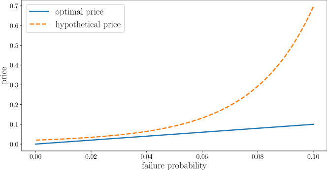
Figure 1. Final good price and failure probabilities.

Thus, returning to the original model, we see that equilibrium prices induce producers to adjust to changes in failure probabilities, which optimally mitigates the potentially exponential impact of failures on the cost of the final good.

4. Application: Knowledge and Communication

Many firms are characterized by a pyramidal structure, in which employees form management layers with each layer smaller than the previous one. These features were modeled by Garicano (2000), where hierarchical organization of knowledge involves a trade-off between the cost of acquiring problem solving knowledge and the cost of communicating with others for help. In this section, we solve a version of Garicano’s model using the dynamic programming theory from Section 2.

Consider a firm where production requires solving a set of problems. Employees at management layer $i$ are assigned problems $m_{i}\in[0,1]$. They learn to solve $z_{i}$ at cost $c(z_{i})$ and pass on the remainder $m_{i+1}=m_{i}-z_{i}$ to the next management layer $i+1$. This incurs additional communication costs that are proportional to the value of problems assigned to layer $i+1$ with coefficient $\tau$.

Let $p\colon[0,1]\to\mathbbm{R}$ be a (fictitious) price function that assigns value to problems. Profits of the $i$th management layer are

$$\pi(m_{i},z_{i})=p(m_{i})-(1+\tau)p(m_{i}-z_{i})-c(z_{i}),$$

where $p(m_{i})$ is the value of problems assigned to layer $i$, $(1+\tau)p(m_{i}-z_{i})$ is the cost of communicating and assigning unsolved problems to the next layer, and $c(z_{i})$ is the cost of learning to solve $z_{i}$. Setting profits to zero and minimizing with respect to $m_{i+1}$ yields

$$p(m_{i})=\min_{m_{i+1}\leqslant m_{i}}\{c(m_{i}-m_{i+1})+(1+\tau)p(m_{i+1})\}.$$

This parallels the Bellman equation (3) of the negative discount dynamic program in Section 2.

Suppose that $n$ employees can learn to solve $z=f(n)$ problems. In other words, for a given range of problems $z$, the number of employees required to solve $z$ is $n=f^{-1}(z)$. Assume that $f$ is strictly increasing, strictly concave, and continuously differentiable with $f(0)=0$, and that $c(z)=wn=wf^{-1}(z)$ for some wage rate $w$. Then the assumptions in (2) are satisfied if we let $\ell=c$ and $\beta=1+\tau$. The Euler equation (EU) implies that the optimal sequence $\{z_{i}\}$ is decreasing, as is the number of employees in each layer as $n_{i}=c(z_{i})/w$. This replicates Garicano’s result that the top management layer has the smallest number of employees and each layer below is larger than the one above.

The Euler equation (EU) adds additional insight: each layer of management acquires knowledge up to the point where the marginal cost of learning equals the marginal cost of communicating and assigning unsolved problems to the next layer. The envelope condition (EN) implies $p^{\prime}(m_{i})=c^{\prime}(z_{i})$, which says that, in equilibrium, the marginal value of problems assigned to a management layer equals the marginal cost of learning to solve problems within the layer.

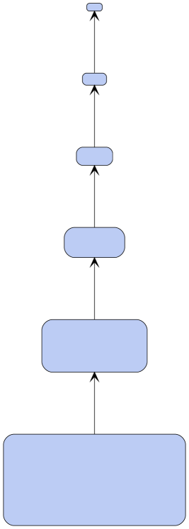
(a) $\tau=0.2$

(b) $\tau=0.4$

(c) $\tau=0.6$

Figure 2. Optimal organizational structures.

Figure 2 plots the optimal organizational structures of three firms given by the model above. Each node corresponds to one management layer, who asks the layer above for help, and its size is proportional to the number of employees in that layer. As shown in the graphs, each firm has a pyramidal structure and higher communication costs increase the relative knowledge acquisition of lower layers and reduce the number of layers.

5. Extension: Nonlinear Networks

In this section we treat more general network models that cannot be directly handled by the theory in Section 2. Unlike the linear chains discussed above, agents can interact with multiple partners. In Section 5.1, we study a problem from economic geography. In Section 5.2 we study chains with multiple upstream partners using a general dynamic programming theory developed in Appendix A.1.

5.1. Spatial Networks

The distribution of city sizes shows remarkable regularity, as described by the rank-size rule. One early attempt to match the empirical city size distribution is found in the central place theory of Christaller (1933). Hsu (2012) and Hsu et al. (2014) formalize Christaller’s theory. In this section, we develop a model with similar insights by extending our earlier dynamic programming results.

Consider a government that opens competition for many developers to build cities to host a continuum of dwellers indexed by $[0,1]$. Each developer can build a large city that hosts everyone or build a smaller city and pay other developers to build “satellite cities” that host the rest of the population. Further satellites can be built for existing cities until all dwellers are accommodated. This chain of city building starts with a single developer, who is assigned the whole population, and ends with a network of cities consisting of multiple layers.

Building satellite cities incurs extra costs that are charged as an ad valorem tax on the payments to the developers. We can think of the extra costs as costs of providing public goods that connect different cities such as roads, electricity, water, telecommunication, etc. Developers are paid according to a price $p\colon[0,1]\to\mathbbm{R}$, which is a function of the population assigned. The cost function of building a city is $c\colon[0,1]\to\mathbbm{R}$ and the tax rate is $\tau$. A developer assigned to host $s$ dwellers maximizes profits by solving

$$\max_{0\leqslant t\leqslant s}\left\{p(s)-c(s-t)-(1+\tau)kp\left(\frac{t}{k}\right)\right\},$$

where $p(s)$ is the payment to the developer, $c(s-t)$ is the cost of building a city of population $s-t$, $k$ is the number of satellite cities, and $(1+\tau)kp(t/k)$ is the cost of assigning population $t/k$ to $k$ satellites. In equilibrium, a city network is formed where every dweller is accommodated and every developer makes zero profits. The equilibrium price function satisfies

$$p(s)=\min_{0\leqslant t\leqslant s}\left\{c(s-t)+(1+\tau)kp\left(\frac{t}{k}\right)\right\}.$$ (13)

To find the equilibrium price function, we first solve a negative discount dynamic program and then show that its value function is the solution to (13).

Consider a dynamic optimization problem with value function given by

$$W(x):=\min_{\{v_{i}\}}\left\{\sum_{i=0}^{\infty}(1+\tau)^{i}k^{i}c(v_{i}):\{v_{i}\}\in\mathbbm{R}_{+}^{\infty}\text{ and }\sum_{i=0}^{\infty}k^{i}v_{i}=x\right\}.$$ (14)

The problem in (14) is a modified version of (1) that also features negative discounting and a convex loss function. In the context of our city network model, (14) describes a social planner who minimizes the total cost of hosting the whole population, where $v_{i}$ stands for the size of cities on layer $i$.

In what follows we let $c(s)=s^{\gamma}$ with $\gamma>1$. To emulate the bifurcation process in Hsu (2012) and Hsu et al. (2014), we let $k=2$. A similar argument to the proof of Proposition 2.3 gives the Euler equation

$$c^{\prime}(v_{i})=(1+\tau)c^{\prime}(v_{i+1}).$$ (15)

Using this equation, it can be shown with some algebra that $v_{i}=\theta^{i}(1-2\theta)$ for $\theta:=(1+\tau)^{1/(1-\gamma)}<1/2$ and the value function is $W(s)=(1-2\theta)^{\gamma-1}s^{\gamma}$. It is straightforward to verify that $p=W$ satisfies (13). Hence, the value function for the social planner is also the equilibrium price function under which all developers make zero profits.

The Euler equation (15) describes the emergence of optimal city hierarchy where each developer expands a city to accommodate more dwellers until the marginal cost of expanding equals the marginal cost of building and expanding satellite cities. An envelope condition similar to (EN) also holds: if a developer is assigned $s$ dwellers and delegate $t$ dwellers to satellite cities, the equilibrium is reached when $p^{\prime}(s)=c^{\prime}(s-t)$. This shows that the marginal value that a city provides must be equal to the marginal cost of accommodating one more city dweller.

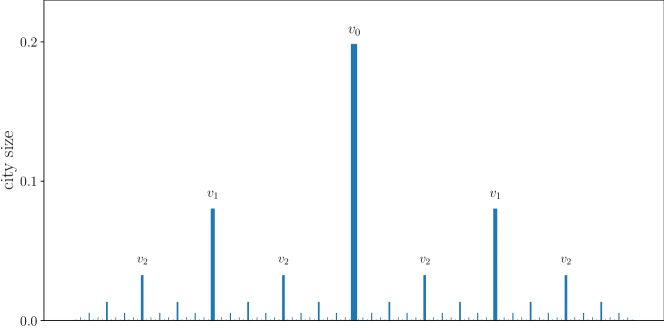
Figure 3. Illustration of optimal city hierarchy.

Figure 3 illustrates the optimal city hierarchy by placing cities according to Hsu (2012) and Hsu et al. (2014). It replicates the relative sizes of cities on different layers as in Hsu (2012) and Hsu et al. (2014). Moreover, since the number of cities doubles from one layer to the next, the rank of a city on layer $i$ is $2^{i}$. Hence, the city size distribution generated by our model follows a power law similar to Hsu (2012). In fact, the rank and size of a city satisfy

$$\ln(Rank)=-\frac{\ln(1/2)}{\ln(\theta)}\ln(Size)+C,$$

where $C$ is a constant determined by $\theta$. When $\theta$ approaches $1/2$, the slope approaches one, which corresponds to the well-documented rank-size rule.

5.2. Snakes and Spiders

Modern production networks are characterized by processes that are both sequential and non-sequential. Baldwin and Venables (2013) refer to the sequential processes as “snakes” and the non-sequential processes as “spiders”, and analyze how the location of different parts of a production chain is determined by unbundling costs of production across borders. Here we study a model of production networks featuring both snakes and spiders.

As in Kikuchi et al. (2018) and Yu and Zhang (2019), we consider a generalization of the production chain model in Section 3.1, where each firm can also choose the number of suppliers. To account for costs of extending spiders, we assume that firms bear an additive assembly cost $g$ that is strictly increasing in the number of suppliers, with $g(1)=0$. Then for a firm at stage $s$ that subcontracts tasks of range $t$ to $k$ suppliers, the profits are

$$p(s)-c(s-t)-g(k)-(1+\tau)kp(t/k),$$

where $p$ is the price function. Having multiple suppliers leads to another trade-off: firms potentially benefit from subcontracting at a lower price but also have to pay additional assembly costs.

We index the layers in the production network by integers $i\geqslant 0$ with layer 0 consisting only of the most downstream firm. Let $b_{i}$ be the downstream boundary of firms on layer $i$, each producing $v_{i}$ and having $k_{i}$ suppliers. Then the boundary of firms on the next layer is given by $b_{i+1}=(b_{i}-v_{i})/k_{i}$. We call $(p,\{v_{i}\},\{k_{i}\})$ an equilibrium for the production network if (i) $p(0)=0$, (ii) $p(s)-c(s-t)-g(k)-(1+\tau)kp(t/k)\leqslant 0$ for all $0\leqslant t\leqslant s\leqslant 1$ and $k\in\mathbbm{N}$, and (iii) $\pi_{i}=0$ for all $i\geqslant 0$ where

$$\pi_{i}:=p(b_{i})-c(v_{i})-g(k_{i})-(1+\tau)k_{i}p\left(\frac{b_{i}-v_{i}}{k_{i}}\right).$$ (16)

As in Section 3.1.2, we seek to find an equilibrium using dynamic programming methods. Let $p^{*}$ be the solution to the following Bellman equation

$$p(s)=\min_{\begin{subarray}{c}0\leqslant t\leqslant s\\ k\in\mathbbm{N}\end{subarray}}\left\{c(s-t)+g(k)+(1+\tau)kp(t/k)\right\}.$$ (17)

Let $v_{i}=b_{i}-t^{*}(b_{i})$ and $k_{i}=k^{*}(b_{i})$ where $t^{*}(s)$ and $k^{*}(s)$ are the minimizers under $p^{*}$. Let $\mathscr{I}$ be all continuous $p$ such that $c^{\prime}(0)s\leqslant p(s)\leqslant c(s)$ for all $s\in[0,1]$.

Proposition 5.1.

If $c^{\prime}(0)>0$ and $g(k)\to\infty$ as $k\to\infty$, then (17) has a unique solution $p^{*}\in\mathscr{I}$ and $(p^{*},\{v_{i}\},\{k_{i}\})$ is an equilibrium for the production network.

In Appendix A.5, we show that the unique solution $p^{*}$ can be computed by value function iteration. We then prove that $p^{*}$ induces an equilibrium allocation. Theorem A.2 can also be used to show the monotonicity of $p^{*}$.

Figure 4 plots two production networks with different transaction costs, where each node corresponds to a firm in the network and the one in the center is the most downstream firm. The size of each node is proportional to the size of the firm, represented by the sum of assembly and transaction costs. Figure 4 shows that more downstream firms are larger and have more upstream suppliers. Comparing panels (A) and (B), we can see that lower transaction costs increase the number of firms involved in the production network, encouraging the expansion of snakes. This is in line with the model prediction of Baldwin and Venables (2013) that decreasing frictions leads to a finer fragmentation of the production.

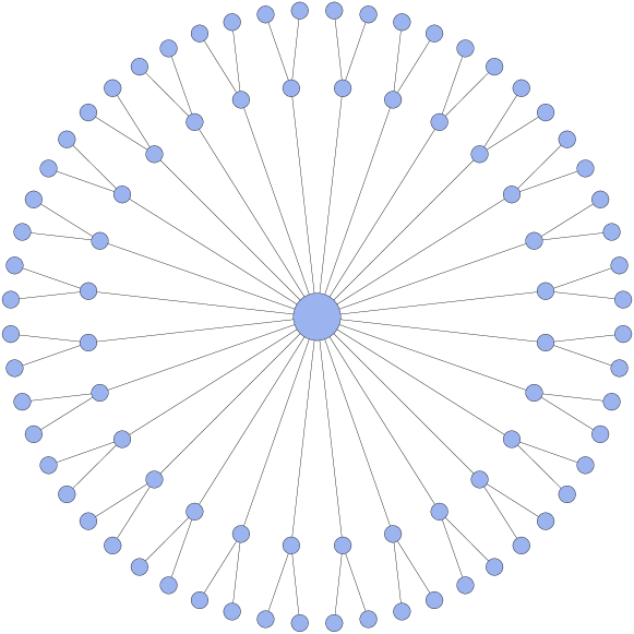
(a) $\tau=0.2$

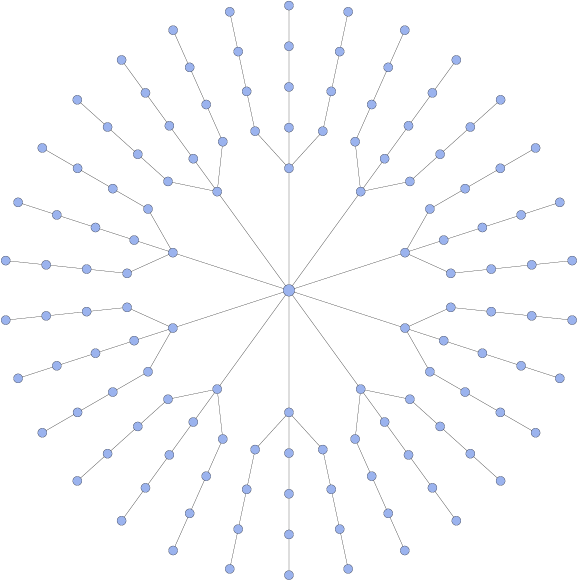
(b) $\tau=0.05$

Figure 4. Examples of production networks.

6. Conclusion

This paper shows how competitive equilibria in a range of production chain and network models can be recovered as solutions to dynamic programming problems. Equilibrium prices are identified with the value function of a dynamic program, while competitive allocations across firms are identified with choices under the optimal policy. Dynamic programming methods are brought to bear on both the theory of the firm and the structure of production networks, providing new insights, as well as new analytical and computational methods. In addition to production problems, we also consider related competitive problems from economic geography and firm management.

Apart from the model of snakes and spiders in Section 5.2, all of the problems faced by individual firms are convex. This assumption allowed us to obtain sharp results and useful characterizations. An important remaining task is to extend our results to a range of cases that feature non-convexities. This work is left for future research.

Appendix A Appendix

A.1. A General Dynamic Programming Framework

In this section, we provide a general dynamic programming framework suitable for analyzing equilibria in production networks.

A.1.1. Set Up

Given a metric space $E$, let $\mathbbm{R}^{E}$ denote the set of functions from $E$ to $\mathbbm{R}$ and let $c\mathbbm{R}^{E}$ be all continuous functions in $\mathbbm{R}^{E}$. Given $g,h\in\mathbbm{R}^{E}$, we write $g\leqslant h$ if $g(x)\leqslant h(x)$ for all $x\in E$, and $\|f\|:=\sup_{x\in E}|f(x)|$.

Let $X$ be a compact metric space. Let $A$ be a metric space and let $G$ be a nonempty, continuous, compact-valued correspondence from $X$ to $A$. We understand $G(x)$ as the set of available actions $a\in A$ for an agent in state $x$. Let $F_{G}:=\{(x,a):x\in X,\;a\in G(x)\}$ be all feasible state-action pairs. Let $L$ be an aggregator, mapping $F_{G}\times\mathbbm{R}^{X}$ into $\mathbbm{R}$, with the interpretation that $L(x,a,w)$ is lifetime loss associated with current state $x$, current action $a$ and continuation value function $w$. A pair $(L,G)$ with these properties is referred to as a dynamic program.

The Bellman operator associated with such a pair is the operator $T$ defined by

$$(Tw)(x)=\inf_{a\in G(x)}L(x,a,w)\qquad(w\in\mathbbm{R}^{X},\;x\in X).$$ (18)

A fixed point of $T$ in $\mathbbm{R}^{X}$ is said to satisfy the Bellman equation.

A.1.2. Fixed Point Results

Fix a dynamic program $(L,G)$ and consider the following assumptions:

• $(x,a)\mapsto L(x,a,w)$ is continuous on $F_{G}$ when $w\in c\mathbbm{R}^{X}$.

• If $u,v\in c\mathbbm{R}^{X}$ with $u\leqslant v$, then $L(x,a,u)\leqslant L(x,a,v)$ for all $(x,a)\in F_{G}$.

• Given $\lambda\in(0,1)$, $u,v\in c\mathbbm{R}^{X}$ and $(x,a)\in F_{G}$, we have

  $$\lambda L(x,a,u)+(1-\lambda)L(x,a,v)\leqslant L(x,a,\lambda u+(1-\lambda)v).$$

• There is a $\psi$ in $c\mathbbm{R}^{X}$ such that $T\psi\leqslant\psi$.

• There is a $\varphi$ in $c\mathbbm{R}^{X}$ and an $\varepsilon>0$ such that $\varphi\leqslant\psi$ and $T\varphi\geqslant\varphi+\varepsilon(\psi-\varphi)$.

Assumptions $A_{1}$–$A_{3}$ impose some continuity, monotonicity and concavity. Assumptions $A_{4}$–$A_{5}$ provide upper and lower bounds for the set of candidate value functions.

Although contractivity is not imposed, we can show that the Bellman operator (18) is well behaved under $A_{1}$–$A_{5}$ after restricting its domain to a suitable class of candidate solutions. To this end, let

$$\mathscr{I}:=\{f\in c\mathbbm{R}^{X}:\varphi\leqslant f\leqslant\psi\}.$$

Theorem A.1.

Let $(L,G)$ be a dynamic program and let $T$ be the Bellman operator defined in (18). If $(L,G)$ satisfies $A_{1}$–$A_{5}$, then

1. $T$ has a unique fixed point $w^{*}$ in $\mathscr{I}$.

2. For each $w\in\mathscr{I}$, there exists an $\alpha<1$ and $M<\infty$ such that

   $$\|T^{n}w-w^{*}\|\leqslant\alpha^{n}M\quad\text{ for all }\,n\in\mathbbm{N}.$$ (19)

3. $\pi^{*}(x):=\operatorname*{arg\,min}_{a\in G(x)}L(x,a,w^{*})$ is upper hemicontinuous on $X$.

The fixed point results in Theorem A.1 rely on the monotonicity and concavity of the Bellman operator. See Section A.2 for details of the arguments and the proof of the theorem.

Theorem A.1 does not discuss Bellman’s principle of optimality. That task is left until Section A.1.4. Regarding $\pi^{*}$, which has the interpretation of a policy correspondence, an immediate corollary is that $\pi^{*}$ is continuous whenever $\pi^{*}$ is single-valued on $X$.

A.1.3. Shape and Smoothness Properties

We now give conditions under which the solution to the Bellman equation associated with a dynamic program possesses additional properties, including monotonicity, convexity and differentiability. In what follows, we assume that $X$ is convex in $\mathbbm{R}$ and $F_{G}$ is convex in $X\times A$. We let

1. $ic\mathbbm{R}^{X}$ be all increasing functions in $c\mathbbm{R}^{X}$ and

2. $cc\mathbbm{R}^{X}$ be all convex functions in $c\mathbbm{R}^{X}$.

We assume that $\mathscr{I}$ defined above contains at least one element of each set. The following assumption is needed for convexity and differentiability.

Assumption A.1.

In addition to $A_{1}$–$A_{5}$, the dynamic program $(L,G)$ satisfies the following conditions:

1. If $w\in cc\mathbbm{R}^{X}$, then $(x,a)\to L(x,a,w)$ is strictly convex on $F_{G}$.

2. If $a\in\operatorname{int}G(x)$ and $w\in cc\mathbbm{R}^{X}$, then $x\to L(x,a,w)$ is differentiable on $\operatorname{int}X$.

We can now state the following result.

Theorem A.2.

If $Tw$ is strictly increasing for all $w\in ic\mathbbm{R}^{X}$, then $w^{*}$ is strictly increasing. If Assumption A.1 holds, then $w^{*}$ is strictly convex, $\pi^{*}$ is single-valued, $w^{*}$ is differentiable on $\operatorname{int}X$ and

$$(w^{*})^{\prime}(x)=L_{x}(x,\pi^{*}(x),w^{*})$$ (20)

whenever $\pi^{*}(x)\in\operatorname{int}G(x)$.

A.1.4. The Principle of Optimality

If we consider the implications of the preceding dynamic programming theory, we have obtained existence of a unique solution to the Bellman equation and certain other properties, but we still lack a definition of optimal policies, and a set of results that connect optimality and solutions to the Bellman equation. This section fills these gaps.

Let $\Pi$ be all $\pi\colon X\to A$ such that $\pi(x)\in G(x)$ for all $x\in X$. For each $\pi\in\Pi$ and $w\in\mathbbm{R}^{X}$, define the operator $T_{\pi}$ by

$$(T_{\pi}w)(x)=L(x,\pi(x),w).$$ (21)

This can be understood as the lifetime loss of an agent following $\pi$ with continuation value $w$. Let $\mathscr{M}$ be the set of (nonstationary) policies, defined as all $\mu=\{\pi_{0},\pi_{1},\ldots\}$ such that $\pi_{t}\in\Pi$ for all $t$. For stationary policy $\{\pi,\pi,\ldots\}$, we simply refer it as $\pi$. Let the $\mu$-value function be defined as

$$w_{\mu}(x):=\limsup_{n\to\infty}(T_{\pi_{0}}T_{\pi_{1}}\ldots T_{\pi_{n}}\varphi)(x),$$ (22)

where $\varphi$ is the lower bound function in $\mathscr{I}$. Note that $w_{\mu}$ is always well defined. The agent’s problem is to minimize $w_{\mu}$ by choosing a policy in $\mathscr{M}$. The value function $\bar{w}$ is defined by

$$\bar{w}(x):=\inf_{\mu\in\mathscr{M}}w_{\mu}(x)$$ (23)

and the optimal policy $\bar{\mu}$ is such that $\bar{w}=w_{\bar{\mu}}$. We impose the following assumption.

Assumption A.2.

In addition to $A_{1}$–$A_{5}$, the dynamic program $(L,G)$ satisfies the following conditions:

1. If $(x,a)\in F_{G}$, $v_{n}\geqslant\varphi$ and $v_{n}\uparrow v$, then $L(x,a,v_{n})\to L(x,a,v)$.

2. There exists a $\beta>0$ such that, for all $(x,a)\in F_{G}$, $r>0$ and $w\geqslant\varphi$,

   $$L(x,a,w+r)\leqslant L(x,a,w)+\beta r.$$ (24)

Part 1 of Assumption A.2 is a weak continuity requirement on the aggregator with respect to the continuation value, similar to Assumption 4 in Bloise and Vailakis (2018). Part 2 of Assumption A.2 is analogous to the Blackwell’s condition, with the significant exception that $\beta$ in (24) is not restricted to be less than one.

Theorem A.3.

If Assumption A.2 holds, then $w^{*}=\bar{w}$ and an optimal stationary policy exists. Moreover, a stationary policy $\pi$ is optimal if and only if $T_{\pi}\bar{w}=T\bar{w}$.

Theorem A.3 shows that the fixed point of the Bellman operator is the value function and the Bellman’s principle of optimality holds. It immediately follows that any selector of $\pi^{*}$ in Theorem A.1 is an optimal stationary policy.

A.2. Proofs for the General Theory

To prove Theorem A.1, we first give a fixed point theorem for monotone concave operators on a partially ordered Banach space due to Du (1989).

Theorem A.4 (Du, 1989).

Let $P$ be a normal cone on a real Banach space $E$. Suppose $u_{0},v_{0}\in E$ with $u_{0}<v_{0}$ and $A:[u_{0},v_{0}]\to E$ is an increasing concave operator. If $Au_{0}\geqslant u_{0}+\varepsilon(v_{0}-u_{0})$ for some $\varepsilon\in(0,1)$ and $Av_{0}\leqslant v_{0}$, then $A$ has a unique fixed point $x^{*}$ in $[u_{0},v_{0}]$. Furthermore, for any $x\in[u_{0},v_{0}]$ and $n\in\mathbbm{N}$, $\|A^{n}x-x^{*}\|\leqslant M(1-\varepsilon)^{n}$ for some $M>0$.

Proof of Theorem A.1.

By $A_{1}$ and Berge’s theorem of the maximum, $Tw$ is continuous. Hence $T$ maps $c\mathbbm{R}^{X}$ to itself. It follows directly from $A_{2}$ that $T$ is isotone on $c\mathbbm{R}^{X}$, in the sense that $u\leqslant v$ implies $Tu\leqslant Tv$. Conditions $A_{4}$–$A_{5}$ and the isotonicity of $T$ imply that, when $\varphi\leqslant w\leqslant\psi$, we have $\varphi\leqslant T\varphi\leqslant Tw\leqslant T\psi\leqslant\psi$. In particular, $T$ is an isotone self-map on $\mathscr{I}$.

The Bellman operator is also concave on $\mathscr{I}$, in the sense that

$$0\leqslant\lambda\leqslant 1\text{ and }u,v\in\mathscr{I}\text{ implies }\lambda Tu+(1-\lambda)Tv\leqslant T(\lambda u+(1-\lambda)v).$$ (25)

Indeed, fixing such $\lambda,u,v$ and applying $A_{3}$, we have

$$\min_{a\in G(x)}\left\{\lambda L(x,a,u)+(1-\lambda)L(x,a,v)\right\}\leqslant\min_{a\in G(x)}L(x,a,\lambda u+(1-\lambda)v)$$

for all $x\in X$. Since, for any pair of real valued functions $f,g$ we have $\min_{a}f(a)+\min_{a}g(a)\leqslant\min_{a}\{f(a)+g(a)\}$, it follows that (25) holds.

The preceding analysis shows that $T$ is an isotone concave self-map on $\mathscr{I}$. In addition, by $A_{4}$ and $A_{5}$, we have $T\psi\leqslant\psi$ and $T\varphi\geqslant\varphi+\varepsilon(\psi-\varphi)$ for some $\varepsilon>0$. Since $\mathscr{I}$ is an order interval in the positive cone of the Banach space $(c\mathbbm{R}^{X},\|\cdot\|)$, and since that cone is normal and solid, the first two claims in Theorem A.1 are now confirmed via Theorem A.4. The final claim is due to Berge’s theorem of the maximum. ∎

Proof of Theorem A.2.

The first part of the theorem follows directly from the fact that $ic\mathbbm{R}^{X}$ is a closed subspace. The proof is omitted. To prove the strict convexity of $w^{*}$, it suffices to show that $Tw$ is strictly convex for all $w\in cc\mathbbm{R}^{X}$ since $cc\mathbbm{R}^{X}$ is a closed subspace of $c\mathbbm{R}^{X}$. Pick any $x_{1},x_{2}\in X$ with $x_{1}<x_{2}$ and any $\lambda\in(0,1)$. Let $x_{\lambda}=\lambda x_{1}+(1-\lambda)x_{2}$. Pick any $w\in cc\mathbbm{R}^{X}$ and let $\pi_{w}\colon X\to A$ be such that $(Tw)(x)=L(x,\pi_{w}(x),w)$. It follows that

$$\lambda(Tw)(x_{1})+(1-\lambda)(Tw)(x_{2}) =\lambda L(x_{1},\pi_{w}(x_{1}),w)+(1-\lambda)L(x_{2},\pi_{w}(x_{2}),w)$$

$$>L(x_{\lambda},\lambda\pi_{w}(x_{1})+(1-\lambda)\pi_{w}(x_{2}),w)$$

$$\geqslant L(x_{\lambda},\pi_{w}(x_{\lambda}),w)=(Tw)(x_{\lambda}),$$

where the first inequality holds because $(x,a)\mapsto L(x,a,w)$ is strictly convex and the second inequality holds because $F_{G}$ is convex. Therefore, $w^{*}$ is strictly convex. Strict convexity of $L$ then implies that $\pi^{*}$ is single-valued.

Since $\pi^{*}(x)\in\operatorname{int}G(x)$ and $G$ is continuous, there exists an open neighborhood $D$ of $x$ such that $\pi^{*}(x)\in\operatorname{int}G(y)$ for all $y\in D$. Define $W(y):=L(y,\pi^{*}(x),w^{*})$ for all $y\in D$. Then $W(y)\geqslant w^{*}(y)$ for all $y\in D$ and $W(x)=w^{*}(x)$. Since $W$ is convex and differentiable on $D$, differentiability of $w^{*}$ and (20) then follow from Benveniste and Scheinkman (1979). ∎

We say that a dynamic programming problem has the monotone increasing property if $-\infty<\varphi(x)\leqslant L(x,a,\varphi)$ for all $(x,a)\in F_{G}$ and Assumption A.2 are satisfied. We state two useful lemmas from Bertsekas (2013).

Lemma A.5 (Proposition 4.3.14, Bertsekas (2013)).

Let the monotone increasing property hold and assume that the sets

$$G_{k}(x,\lambda):=\{x\in G(x)\mid L(x,a,T^{k}\varphi)\leqslant\lambda\}$$

are compact for all $x\in X$, $\lambda\in\mathbbm{R}$, and $k$ greater than some integer $\bar{k}$. If $w\in\mathbbm{R}_{+}^{X}$ satisfies $\varphi\leqslant w\leqslant\bar{w}$, then $\lim_{n\to\infty}T^{n}w=\bar{w}$. Furthermore, there exists an optimal stationary policy.

Lemma A.6 (Proposition 4.3.9, Bertsekas (2013)).

Under the monotone increasing property, a stationary policy $\pi$ is optimal if and only if $T_{\pi}\bar{w}=T\bar{w}$.

Proof of Theorem A.3.

Theorem A.1 implies that $\lim_{n\to\infty}T^{n}\varphi=w^{*}$. To prove $w^{*}=\bar{w}$, it suffices to show that the conditions of Lemma A.5 hold and $\varphi\leqslant\bar{w}$.

It follows from $A_{5}$ that $\varphi(x)\leqslant(T\varphi)(x)\leqslant L(x,a,\varphi)$ for all $(x,a)\in F_{G}$. Therefore, the monotone increasing property is satisfied. Since $T$ is a self-map on $c\mathbbm{R}^{X}$, to check the conditions of Lemma A.5, it suffices to prove that the set

$$G(x,\lambda):=\{x\in G(x)\mid L(x,a,w)\leqslant\lambda\}$$

is compact for any $w\in c\mathbbm{R}^{X}$, $x\in X$, and $\lambda\in\mathbbm{R}$. Since $a\mapsto L(x,a,w)$ is continuous by $A_{1}$, $L(x,\cdot\,,w)^{-1}\left((-\infty,\lambda]\right)$ is a closed set. Since $G$ is compact-valued, $G(x,\lambda)$ is compact. It remains to show that $\varphi\leqslant\bar{w}$. By $A_{2}$ and the monotone increasing property, we have for any $\mu=(\pi_{0},\pi_{1},\ldots)\in\mathscr{M}$, $\varphi\leqslant T_{\pi_{0}}T_{\pi_{1}}\ldots T_{\pi_{n}}\varphi$ for all $n\in\mathbbm{N}$. Then by definition, $\varphi\leqslant w_{\mu}$ for all $\mu\in\mathscr{M}$. Taking the infimum gives $\varphi\leqslant\bar{w}$. Lemma A.5 then implies that $w^{*}=\bar{w}$ and there exists an optimal stationary policy. The principle of optimality follows directly from Lemma A.6. ∎

A.3. Proofs for Section 2

Let $\mathscr{F}$ be the set of increasing convex functions in $\mathscr{I}$. Throughout the proofs, we regularly use the alternative expression for $T$ given by

$$(Tw)(x)=\min_{0\leqslant y\leqslant x}\,\{\ell(x-y)+\beta w(y)\}.$$ (26)

Also, given $w\in\mathscr{F}$, define

$$\pi_{w}(x)=\operatorname*{arg\,min}_{0\leqslant a\leqslant x}\,\{\ell(a)+\beta w(x-a)\}$$

and

$$\sigma_{w}(x):=\operatorname*{arg\,min}_{0\leqslant y\leqslant x}\{\ell(x-y)+\beta w(y)\}=x-\pi_{w}(x).$$ (27)

These functions are clearly well-defined, unique and single-valued. Let $\sigma=\sigma_{w^{*}}$ and $\pi=\pi_{w^{*}}$. Let $\eta$ be the constant defined by

$$\eta:=\max\,\{0\leqslant x\leqslant\hat{x}:\ell^{\prime}(x)\leqslant\beta\ell^{\prime}(0)\}.$$ (28)

We begin with several lemmas. The proof of the first lemma is trivial and hence omitted.

Lemma A.7.

We have $\eta>0$ if and only if $\ell^{\prime}(0)>0$. If $\eta<\hat{x}$, then $\ell^{\prime}(\eta)=\beta\ell^{\prime}(0)$.

Lemma A.8.

If $w\in\mathscr{F}$, then $\sigma_{w}(x)=0$ if and only if $x\leqslant\eta$.

Proof.

First suppose that $x\leqslant\eta$. Seeking a contradiction, suppose there exists a $y\in(0,x]$ such that $\ell(x-y)+\beta w(y)<\ell(x)$. Since $w\in\mathscr{F}$ we have $w(y)\geqslant\ell^{\prime}(0)y$ and hence

$$\beta w(y)\geqslant\beta\ell^{\prime}(0)y\geqslant\ell^{\prime}(\eta)y.$$

Since $x\leqslant\eta$, this implies that $\beta w(y)\geqslant\ell^{\prime}(x)y$. Combining these inequalities gives $\ell(x-y)+\ell^{\prime}(x)y<\ell(x)$, contradicting convexity of $\ell$.

Now suppose that $\sigma_{w}(x)=0$. We claim that $x\leqslant\eta$, or, equivalently $\ell^{\prime}(x)\leqslant\beta\ell^{\prime}(0)$. To prove $\ell^{\prime}(x)\leqslant\beta\ell^{\prime}(0)$, observe that since $w\in\mathscr{F}$ we have $w(y)\leqslant\ell(y)$, and hence

$$\ell(x)\leqslant\ell(x-y)+\beta w(y)\leqslant\ell(x-y)+\beta\ell(y)\quad\text{for all }y\leqslant x.$$

It follows that

$$\frac{\ell(x)-\ell(x-y)}{y}\leqslant\frac{\beta\ell(y)}{y}\quad\text{for all}\quad y\leqslant x.$$

Taking the limit gives $\ell^{\prime}(x)\leqslant\beta\ell^{\prime}(0)$. ∎

Proof of Proposition 2.1.

Let $A=X=[0,\hat{x}]$, $G(x)=[0,x]$ and $L(x,a,w)=\ell(a)+\beta w(x-a)$. Conditions $A_{1}$–$A_{3}$ in Section A.1.2 obviously hold. Condition $A_{4}$ holds since $\min_{0\leqslant a\leqslant x}\{\ell(a)+\beta\ell(x-a)\}\leqslant\ell(x)$. For condition $A_{5}$, note that $L(x,a,\varphi)=\ell(a)+\beta\ell^{\prime}(0)(x-a)$. Then $T\varphi=\ell$ if $x<\eta$ and $(T\varphi)(x)=\ell(\eta)+\beta\ell^{\prime}(0)(x-\eta)$ if $x\geqslant\eta$. For $x<\eta$, $T\varphi-\varphi=\psi-\varphi$ so we can choose any $\varepsilon\leqslant 1$. For $x\geqslant\eta$,

$$(T\varphi)(x)-\varphi(x) =\ell(\eta)+\beta\ell^{\prime}(0)(x-\eta)-\ell^{\prime}(0)x$$

$$=\ell(\eta)-\ell^{\prime}(0)\eta+(\beta-1)\ell^{\prime}(0)(x-\eta)$$

$$\geqslant\ell(\eta)-\ell^{\prime}(0)\eta=(\psi-\varphi)(\eta).$$

Since $\psi-\varphi$ is increasing, we can choose any $\varepsilon\leqslant\bar{\varepsilon}$ where $(\psi-\varphi)(\eta)=\bar{\varepsilon}(\psi-\varphi)(\hat{x})$. The first part of the proposition thus follows from Theorem A.1.

Consider the alternative expression for $T$ in (26). Since $\ell$ is strictly convex, $(x,y)\mapsto\ell(x-y)+\beta w(y)$ is strictly convex for all $w\in cc\mathbbm{R}^{X}$. Hence, part 1 of Assumption A.1 holds. Evidently $Tw$ is strictly convex for all $w\in\mathscr{F}$.

Next we show that $Tw$ is strictly increasing for all $w\in\mathscr{F}$. Pick any $w\in\mathscr{F}$ and $x_{1}\leqslant x_{2}$. For ease of notation, let $y_{i}=\sigma_{w}(x_{i})$ for $i\in\{1,2\}$. If $y_{2}\leqslant x_{1}$, then

$$(Tw)(x_{1}) =\ell(x_{1}-y_{1})+\beta w(y_{1})$$

$$\leqslant\ell(x_{1}-y_{2})+\beta w(y_{2})$$

$$<\ell(x_{2}-y_{2})+\beta w(y_{2})=(Tw)(x_{2}),$$

where the first inequality holds since $y_{2}$ is available when $y_{1}$ is chosen and the second inequality holds since $\ell$ is strictly increasing. If $y_{2}>x_{1}$, we first consider the case of $x_{1}+y_{2}<x_{2}$. Then $(Tw)(x_{2})>\ell(x_{1})+\beta w(y_{2})\geqslant\ell(x_{1})\geqslant(Tw)(x_{1})$. For the case of $x_{1}+y_{2}\geqslant x_{2}$, we have $0\leqslant y_{1}^{\prime}\leqslant x_{1}<y_{2}$ where $y_{1}^{\prime}=x_{1}+y_{2}-x_{2}$. Since $w$ is not constant, $w\in\mathscr{F}$ implies that $w$ is strictly increasing. It follows that

$$(Tw)(x_{1}) =\ell(x_{1}-y_{1})+\beta w(y_{1})$$

$$\leqslant\ell(x_{1}-y_{1}^{\prime})+\beta w(y_{1}^{\prime})$$

$$<\ell(x_{2}-y_{2})+\beta w(y_{2})=(Tw)(x_{2}).$$

Therefore, $T$ is a self-map on $\mathscr{F}$ and $Tw$ is strictly increasing and strictly convex for all $w\in\mathscr{F}$. Theorem A.2 then implies that $w^{*}$ is strictly increasing and strictly convex.

Since $\ell$ is differentiable, part 2 of Assumption A.1 holds. Theorem A.2 then implies that $w^{*}$ is differentiable and $(w^{*})^{\prime}(x)=\ell^{\prime}(x-\sigma(x))$ whenever $\sigma(x)$ is interior. Lemma A.8 implies that $w^{*}(x)=\ell(x)$ and thus $(w^{*})^{\prime}(x)=\ell^{\prime}(x)$ when $x\leqslant\eta$; when $x>\eta$, $\sigma$ is interior and $(w^{*})^{\prime}(x)=\ell^{\prime}(x-\sigma(x))$. Since $\sigma$ is continuous, $(w^{*})^{\prime}$ is continuous. Therefore, $w^{*}$ is continuously differentiable on $(0,\hat{x})$ and $(w^{*})^{\prime}(x)=\ell^{\prime}(\pi(x))$. ∎

The next lemma further characterizes $\pi$ and $\sigma$.

Lemma A.9.

Let $w\in\mathscr{F}$. If $x_{1},x_{2}$ satisfy $0<x_{1}\leqslant x_{2}$, then $\sigma_{w}(x_{1})\leqslant\sigma_{w}(x_{2})$ and $\pi_{w}(x_{1})\leqslant\pi_{w}(x_{2})$. Moreover, if $x\geqslant\eta$, then $\pi_{w}(x)\geqslant\eta$; if $x\leqslant\eta$, then $\pi_{w}(x)=x$.

Proof.

Pick any $w\in\mathscr{F}$. Since $\ell$ and $w$ are convex, the maps $(x,a)\mapsto\ell(a)+\beta w(x-a)$ and $(x,y)\mapsto\ell(x-y)+\beta w(y)$ both satisfy the single crossing property. It follows from Theorem $4^{\prime}$ of Milgrom and Shannon (1994) that $\pi_{w}$ and $\sigma_{w}$ are increasing.

For the last claim, since $\pi_{w}$ is increasing, Lemma A.8 implies that, if $\eta\leqslant x$, then $\pi_{w}(x)\geqslant\pi_{w}(\eta)=\eta-\sigma_{w}(\eta)=\eta$; and if $x\leqslant\eta$, then $\pi_{w}(x)=x-\sigma_{w}(x)=x$. ∎

The following lemma characterizes the solution to (1) and is useful when showing the equivalence between (1) and (3).

Lemma A.10.

If $\{a_{t}\}$ is a solution to (1), then $\{a_{t}\}$ is monotone decreasing and $a_{T+1}=0$ if and only if $a_{T}\leqslant\eta$.

Proof.

The first claim is obvious, because if $\{a_{t}\}$ is a solution to (1) with $a_{t}<a_{t+1}$, then, given that $\beta>1$, swapping the values of these two points in the sequence will preserve the constraint while strictly decreasing total loss. Regarding the second claim, since $\{a_{t}\}$ is monotone decreasing, it suffices to check the case $a_{T}>0$. To this end, suppose to the contrary that $\{a_{t}\}$ is a solution to (1) with $0<a_{T}<\eta$ and $a_{T+1}>0$. Consider an alternative feasible sequence $\{\hat{a}_{t}\}$ defined by $\hat{a}_{T}=a_{T}+\varepsilon$, $\hat{a}_{T+1}=a_{T+1}-\varepsilon$ and $\hat{a}_{t}=a_{t}$ for other $t$. If we compare the values of these two sequences we get

$$\sum_{t=0}^{\infty}\beta^{t}\ell(a_{t})-\sum_{t=0}^{\infty}\beta^{t}\ell(\hat{a}_{t}) =\beta^{T}[\ell(a_{T})-\ell(a_{T}+\varepsilon)]+\beta^{T+1}[\ell(a_{T+1})-\ell(a_{T+1}-\varepsilon)]$$

$$=\varepsilon\beta^{T}\left\{-\frac{\ell(a_{T}+\varepsilon)-\ell(a_{T})}{\varepsilon}+\beta\frac{\ell(a_{T+1}-\varepsilon)-\ell(a_{T+1})}{-\varepsilon}\right\}.$$

The term inside the parenthesis converges to

$$-\ell^{\prime}(a_{T})+\beta\ell^{\prime}(a_{T+1})>-\ell^{\prime}(\eta)+\beta\ell^{\prime}(0)\geqslant 0,$$

where the first inequality follows from $a_{T}\leqslant\eta$, $a_{T+1}>0$ and strict convexity of $\ell$; and the second inequality is by the definition of $\eta$. We conclude that for $\varepsilon$ sufficiently small, the difference $\sum_{t=0}^{\infty}\beta^{t}\ell(a_{t})-\sum_{t=0}^{\infty}\beta^{t}\ell(\hat{a}_{t})$ is positive, contradicting optimality.

Finally we check the claim $a_{T+1}=0\implies a_{T}\leqslant\eta$. Note that if $\eta=\hat{x}$ then there is nothing to prove, so we can and do take $\eta<\hat{x}$. Seeking a contradiction, suppose instead that $a_{T+1}=0$ and $a_{T}>\eta$. Consider an alternative feasible sequence $\{\hat{a}_{t}\}$ defined by $\hat{a}_{T}=a_{T}-\varepsilon$, $\hat{a}_{T+1}=\varepsilon$ and $\hat{a}_{t}=a_{t}$ for other $t$. In this case we have

$$\sum_{t=0}^{\infty}\beta^{t}\ell(a_{t})-\sum_{t=0}^{\infty}\beta^{t}\ell(\hat{a}_{t})=\varepsilon\beta^{T}\left\{\frac{\ell(a_{T}-\varepsilon)-\ell(a_{T})}{-\varepsilon}-\beta\frac{\ell(\varepsilon)-\ell(0)}{\varepsilon}\right\}.$$

The term inside the parentheses converges to

$$\ell^{\prime}(a_{T})-\beta\ell^{\prime}(0)>\ell^{\prime}(\eta)-\beta\ell^{\prime}(0)=0,$$

where the final equality is due to $\eta<\hat{x}$ and Lemma A.7. Once again we conclude that for $\varepsilon$ sufficiently small, the difference $\sum_{t=0}^{\infty}\beta^{t}\ell(a_{t})-\sum_{t=0}^{\infty}\beta^{t}\ell(\hat{a}_{t})$ is positive, contradicting optimality. ∎

Proof of Proposition 2.2.

To show the equivalence between (1) and (3), we first show that (1) is equivalent to $\bar{w}=\inf_{\mu\in\mathscr{M}}w_{\mu}$ where $w_{\mu}$ is as defined in (22). Suppose that the optimal policy is $\mu=(\pi_{0},\pi_{1},\ldots)$ and we let $\sigma_{t}(x)=x-\pi_{t}(x)$. Then we have

$$\bar{w}(\hat{x})=w_{\mu}(\hat{x})=\ell[\pi_{0}(\hat{x})]+\beta\ell[\pi_{1}\sigma_{0}(\hat{x})]+\beta^{2}\ell[\pi_{2}\sigma_{1}\sigma_{0}(\hat{x})]+\ldots\\ +\limsup_{t\to\infty}\beta^{k}\ell^{\prime}(0)\sigma_{t-1}\sigma_{t-2}\cdots\sigma_{0}(\hat{x}).$$ (29)

It is clear that $\bar{w}$ is finite. Therefore, the optimal policy must satisfy $\sigma_{t}\to 0$, otherwise the last term in (29) would go to infinity. Let $a_{t}=\pi_{t}\sigma_{t-1}\ldots\sigma_{0}(\hat{x})$. We claim that $\{a_{t}\}$ solves (1). Suppose not and the solution to (1) is $\{a^{\prime}_{t}\}$. Then by Lemma A.10, $a^{\prime}_{t}=0$ for all $t>T$ for some $T$. Thus we can construct a policy $\mu^{\prime}$ that reproduces $\{a_{t}^{\prime}\}$ and gives a lower loss. This is a contradiction. Conversely, suppose that the solution to (1) is $\{a_{t}\}$. Using the same argument, we can show that the policy that gives rise to $\{a_{t}\}$ is an optimal policy. Therefore, $W=\bar{w}$.

Next we show that $w^{*}=\bar{w}$ using Theorem A.3. Both conditions in Assumption A.2 can be verified for $(L,G)$. Part 1 of Assumption A.2 is trivial in this setting, since $v_{n}\uparrow v$ pointwise clearly implies $\ell(a)+\beta v_{n}(x-a)\to\ell(a)+\beta v(x-a)$ at each $(x,a)\in F_{G}$. Part 2 also holds, since for any $r>0$ and $w\geqslant\varphi$, we have

$$L(x,a,w+r)=\ell(a)+\beta w(x-a)+\beta r=L(x,a,w)+\beta r.$$

Hence Theorem A.3 applies. It follows from Theorem A.3 that $w^{*}=\bar{w}$, there exists an stationary optimal policy, and the Bellman’s principle of optimality holds. Since $\pi^{*}$ satisfies $T_{\pi^{*}}w^{*}=Tw^{*}$, $\pi^{*}$ is a stationary optimal policy.

Theorems A.1 and A.2 imply that $\pi^{*}$ is continuous and single-valued. It then follows from the principle of optimality that $\{a_{t}^{*}\}$ is the unique solution to (1). ∎

Proposition A.11.

For all $n\in\mathbbm{N}$ and increasing convex $w\in\mathscr{I}$, we have

$$T^{n}w(x)=w^{*}(x)\;\text{ whenever }\,x\leqslant n\eta.$$

Proposition A.11 implies uniform convergence in finite time. In particular, for $n\geqslant\hat{x}/\eta$ we have $T^{n}w=w^{*}$ everywhere on $[0,\hat{x}]$. Note that this bound $\hat{x}/\eta$ is independent of the initial condition $w$.

Proof of Proposition A.11.

It suffices to show that if $f,g\in\mathscr{F}$, then $T^{k}f=T^{k}g$ on $[0,k\eta]$. We prove this by induction.

To see that $T^{1}f=T^{1}g$ on $[0,\eta]$, pick any $x\in[0,\eta]$ and recall from Lemma A.8 that if $h\in\mathscr{F}$ and $x\leqslant\eta$, then $Th(x)=\ell(x)$. Applying this result to both $f$ and $g$ gives $Tf(x)=Tg(x)=\ell(x)$. Hence $T^{1}f=T^{1}g$ on $[0,\eta]$ as claimed.

Turning to the induction step, suppose now that $T^{k}f=T^{k}g$ on $[0,k\eta]$, and pick any $x\in[0,(k+1)\eta]$. Let $h\in\mathscr{F}$ be arbitrary, let $\pi_{h}$ be the $h$-greedy function, and let $\sigma_{h}(x):=x-\pi_{h}(x)$. By Lemma A.9, we have $\pi_{h}(x)\geqslant\eta$, and hence

$$\sigma_{h}(x)\leqslant x-\eta\leqslant(k+1)\eta-\eta\leqslant k\eta.$$

In other words, given function $h$, the optimal choice at $x$ is less than $k\eta$. Since this is true for both $h=T^{k}f$ and $h=T^{k}g$, we have

$$T^{k+1}f(x)=\min_{0\leqslant y\leqslant x}\{\ell(x-y)+\beta T^{k}f(y)\}=\min_{0\leqslant y\leqslant k\eta}\{\ell(x-y)+\beta T^{k}f(y)\}.$$

Using the induction step we can now write

$$T^{k+1}f(x)=\min_{0\leqslant y\leqslant k\eta}\{\ell(x-y)+\beta T^{k}g(y)\}=\min_{0\leqslant y\leqslant x}\{\ell(x-y)+\beta T^{k}g(y)\}.$$

The last expression is just $T^{k+1}g(x)$, and we have now shown that $T^{k+1}f=T^{k+1}g$ on $[0,(k+1)\eta]$. The proof is complete. ∎

Proof of Proposition 2.3.

Since $\ell^{\prime}(0)=0$, (EU) is equivalent to $\beta\ell^{\prime}(a^{*}_{t+1})=\ell^{\prime}(a^{*}_{t})$.

Sufficiency. Let $x_{0}^{*}=\hat{x}$ and $x_{t}^{*}=x_{t-1}^{*}-a_{t-1}^{*}$ for $t\geqslant 1$. Let $\{a_{t}\}$ be any feasible sequence. Let $x_{0}=\hat{x}$ and $x_{t}=x_{t-1}-a_{t-1}$. It suffices to prove that

$$D:=\lim_{T\to\infty}\sum_{t=0}^{T}\beta^{t}[\ell(a_{t}^{*})-\ell(a_{t})]\leqslant 0.$$

Since $\ell$ is convex, we have

$$D=\lim_{T\to\infty}\sum_{t=0}^{T}\beta^{t}[\ell(x_{t}^{*}-x_{t+1}^{*})-\ell(x_{t}-x_{t+1})]\leqslant\lim_{T\to\infty}\sum_{t=0}^{T}\beta^{t}\ell^{\prime}(a_{t}^{*})(x_{t}^{*}-x_{t}-x_{t+1}^{*}+x_{t+1}).$$

Since $x_{0}=x_{0}^{*}$, rearranging gives

$$D\leqslant\lim_{T\to\infty}\sum_{t=0}^{T}\beta^{t}(x_{t+1}^{*}-x_{t+1})[\beta\ell^{\prime}(a_{t+1}^{*})-\ell^{\prime}(a_{t}^{*})]-\beta^{T}\ell^{\prime}(a_{T}^{*})(x_{T+1}^{*}-x_{T+1}).$$

Since $\beta\ell^{\prime}(a_{t+1}^{*})=\ell^{\prime}(a_{t}^{*})$, the summation is zero and $\beta^{T}\ell^{\prime}(a_{T}^{*})=\ell^{\prime}(a_{0}^{*})$. We have

$$D\leqslant-\lim_{T\to\infty}\ell^{\prime}(a_{0}^{*})(x_{T+1}^{*}-x_{T+1}).$$

Since $\{a_{t}\}$ and $\{a_{t}^{*}\}$ are feasible, $x_{T+1}$ and $x_{T+1}^{*}$ go to zero as $T\to\infty$. Hence $D\leqslant 0$.

Existence and Uniqueness. Since $\{a_{t}^{*}\}$ is feasible and satisfies $\beta\ell^{\prime}(a_{t+1}^{*})=\ell^{\prime}(a_{t}^{*})$ for all $t$, we have

$$\hat{x}=\sum_{t=0}^{\infty}a_{t}^{*}=\sum_{t=0}^{\infty}(\ell^{\prime})^{-1}\left(\frac{1}{\beta^{t}}\ell^{\prime}(a_{0}^{*})\right)=:g(a_{0}^{*}),$$

where $(\ell^{\prime})^{-1}$ is well defined on $[0,\lim_{x\to\infty}\ell^{\prime}(x)]$ because $\ell$ is increasing, strictly convex, and $\ell^{\prime}(0)=0$. Hence, $g$ is well defined on $\mathbbm{R}_{+}$ and $g(a_{0}^{*})$ is continuous and strictly increasing in $a_{0}^{*}$. Since $g(0)=0$ and $g(\hat{x})>\hat{x}$, there exists a unique $a_{0}^{*}>0$ such that $\{a_{t}^{*}\}$ satisfying $\beta\ell^{\prime}(a_{t+1}^{*})=\ell^{\prime}(a_{t}^{*})$ is feasible, $a_{t}^{*}>0$ for all $t$, and $\{a_{t}^{*}\}$ is strictly decreasing. That $\{a_{t}^{*}\}$ is an optimal solution then follows from the sufficiency part. Since $\ell$ is strictly convex, the solution is unique.

Necessity. Since we have pinned down a unique solution of (1) which satisfies $\beta\ell^{\prime}(a_{t+1}^{*})=\ell^{\prime}(a_{t}^{*})$, the condition is also necessary. ∎

A.4. Proofs for Section 3

Proof of Proposition 3.1.

We must verify that $(W,\{a_{i}^{*}\})$ satisfies Definition 3.1. We first consider the case of $\ell^{\prime}(0)>0$. By Propositions 2.1 and 2.2, the value function $W$ is a solution to the Bellman equation (3), and hence satisfies

$$W(s)=\min_{0\leqslant v\leqslant s}\,\{c(v)+(1+\tau)W(s-v)\}\quad\text{for all }s\in[0,1],$$ (30)

and $W$ lies in the class $\mathscr{F}$ of increasing, convex and continuous functions $f\colon\mathbbm{R}_{+}\to\mathbbm{R}_{+}$ such that $c^{\prime}(0)s\leqslant f(s)\leqslant c(s)$ for all $s\in\mathbbm{R}_{+}$. In addition, with $\{x_{i}\}$ as the optimal state process (see Proposition 2.2), we have,

$$W(x_{i})=\{c(a^{*}_{i})+(1+\tau)W(x_{i+1})\}\quad\text{for all }i\geqslant 0.$$ (31)

We need to show that 1–3 of Definition 3.1 hold when $p=W$ and $v_{i}=a_{i}^{*}$ for all $i\geqslant 0$. Part 1 is immediate because $W\in\mathscr{F}$ and all functions in $\mathscr{F}$ must have this property, while Part 2 follows directly from (30). To see that Part 3 of Definition 3.1 also holds, let $b_{i}=x_{i}$. By the definition of the state process, the sequence $\{b_{i}\}$ then corresponds to the downstream boundaries of a set of firms obeying task allocation $\{a_{i}^{*}\}$. The profits of firm $i$ are $\pi_{i}=W(b_{i})-c(a^{*}_{i})-(1+\tau)W(b_{i+1})$. By (31) and $b_{i}=x_{i}$, we have $\pi_{i}=0$ for all $i$. Hence Part 3 of Definition 3.1 also holds, as was to be shown.

If $\ell^{\prime}(0)=0$, part 1 follows from the definition of the value function (6). By Proposition 2.3, for any $t$ with $0\leqslant t\leqslant 1$, there exists a unique optimal allocation $\{a_{t,j}^{*}\}$ such that $W(t)=\sum_{j}\beta^{j}\ell(a_{t,j}^{*})$, and $\sum_{j}a_{t,j}^{*}=t$. Since $\{s-t,a_{t,0}^{*},a_{t,1}^{*},\ldots\}$ is a feasible allocation at stage $s$ with $t\leqslant s\leqslant 1$, part 2 follows from the definition of the value function. To see part 3, let $b_{0}=1$ and $b_{i}=b_{i-1}-a_{i-1}^{*}$. By Proposition 2.3, we have $\ell^{\prime}(a_{i}^{*})=(1+\tau)\ell^{\prime}(a_{i+1}^{*})$. Since $\sum_{i=j}^{\infty}a_{i}^{*}=b_{j}$ for all $j$, it follows again from Proposition 2.3 that $\{a_{i}^{*}\}_{i=j}^{\infty}$ is an optimal allocation for stage $b_{j}$. Therefore, $p(b_{i})=\sum_{j=0}^{\infty}(1+\tau)^{j}c(a_{i+j}^{*})=c(a_{i}^{*})+(1+\tau)p(b_{i+1})$ for all $i$. Hence, $\pi_{i}=0$ for all $i$. ∎

A.5. Proofs for Section 5

Proof of Proposition 5.1.

To study this problem in the framework of Section A.1, we set $X=[0,\hat{x}]$, $A=[0,\hat{x}]\times\mathbbm{N}$, $G(x)=[0,x]\times\mathbbm{N}$, and

$$L(x,a,w)=c(x-t)+g(k)+(1+\tau)kp(t/k)\qquad a=(t,k).$$

Since $g(k)\to\infty$ as $k\to\infty$, we can restrict $G(x)$ to be $[0,x]\times\{1,2,\ldots,\bar{k}\}$ so that $G$ is compact-valued. Under the conditions of Proposition 5.1, it can be shown that $A_{1}$–$A_{5}$ hold with $\psi=c$ and $\varphi(s)=c^{\prime}(0)s$ (see Yu and Zhang (2019)). Then, Theorem A.1 implies that the Bellman equation (17) has a unique solution $p^{*}$ in $\mathscr{I}$, $T^{n}p\to p^{*}$ for all $p\in\mathscr{I}$ where

$$(Tp)(s):=\min_{\begin{subarray}{c}0\leqslant t\leqslant s\\ k\in\mathbbm{N}\end{subarray}}L(x,a,w),$$

and $t^{*}$ and $k^{*}$ exist. We need only verify that $(p^{*},\{v_{i}\},\{k_{i}\})$ given by $v_{i}=b_{i}-t^{*}(b_{i})$, $k_{i}=k^{*}(b_{i})$ and $b_{i+1}=(b_{i}-v_{i})/k_{i}$ is an equilibrium, the definition of which is given in Section 5.2.

Since $p^{*}\in\mathscr{I}$, $p(0)=0$. Since $p^{*}$ satisfies (17), part (ii) of the definition is also satisfied. To see that part (iii) holds, note that

$$p^{*}(b_{i}) =c(b_{i}-t^{*}(b_{i}))+g(k^{*}(b_{i}))+(1+\tau)k^{*}(b_{i})p^{*}\left(\frac{t^{*}(b_{i})}{k^{*}(b_{i})}\right)$$

$$=c(v_{i})+g(k_{i})+(1+\tau)k_{i}p^{*}\left(\frac{b_{i}-v_{i}}{k_{i}}\right).$$

It follows that $\pi_{i}=0$ for all $i\in\mathbbm{Z}$ where $\pi_{i}$ is as defined in (16). This completes the proof. ∎

References

- Antràs and De Gortari (2020) Antràs, P. and A. De Gortari (2020): “On the geography of global value chains,” Econometrica, 88, 1553–1598.
- Baldwin and Venables (2013) Baldwin, R. and A. J. Venables (2013): “Spiders and snakes: offshoring and agglomeration in the global economy,” Journal of International Economics, 90, 245–254.
- Benveniste and Scheinkman (1979) Benveniste, L. M. and J. A. Scheinkman (1979): “On the differentiability of the value function in dynamic models of economics,” Econometrica, 47, 727–732.
- Bertsekas (2013) Bertsekas, D. P. (2013): Abstract Dynamic Programming, Athena Scientific Belmont, MA.
- Bloise and Vailakis (2018) Bloise, G. and Y. Vailakis (2018): “Convex dynamic programming with (bounded) recursive utility,” Journal of Economic Theory, 173, 118–141.
- Boehm and Oberfield (2020) Boehm, J. and E. Oberfield (2020): “Misallocation in the market for inputs: enforcement and the organization of production,” The Quarterly Journal of Economics, 135, 2007–2058.
- Christaller (1933) Christaller, W. (1933): Central Places in Southern Germany, Translation into English by Carlisle W. Baskin in 1966, Englewood Cliffs, NJ: Prentice-Hall.
- Coase (1937) Coase, R. H. (1937): “The nature of the firm,” Economica, 4, 386–405.
- Coe and Yeung (2015) Coe, N. M. and H. W.-C. Yeung (2015): Global Production Networks: Theorizing Economic Development in an Interconnected World, Oxford University Press.
- Costinot et al. (2013) Costinot, A., J. Vogel, and S. Wang (2013): “An elementary theory of global supply chains,” The Review of Economic Studies, 80, 109–144.
- Du (1989) Du, Y. (1989): “Fixed points of a class of non-compact operators and applications,” Acta Mathematica Sinica, 32, 618–627.
- Epstein and Zin (1989) Epstein, L. and S. Zin (1989): “Substitution, risk aversion, and the temporal behavior of consumption and asset returns: a theoretical framework,” Econometrica, 57, 937–69.
- Fally and Hillberry (2018) Fally, T. and R. Hillberry (2018): “A Coasian model of international production chains,” Journal of International Economics, 114, 299–315.
- Farlow (2020) Farlow, A. (2020): “Beyond COVID-19: Supply Chain Resilience Holds Key to Recovery,” Tech. rep., Baker McKenzie.
- Gabaix (2009) Gabaix, X. (2009): “Power laws in economics and finance,” Annu. Rev. Econ., 1, 255–294.
- Gabaix and Ioannides (2004) Gabaix, X. and Y. M. Ioannides (2004): “The evolution of city size distributions,” in Handbook of Regional and Urban Economics, Elsevier, vol. 4, 2341–2378.
- Garicano (2000) Garicano, L. (2000): “Hierarchies and the organization of knowledge in production,” Journal of Political Economy, 108, 874–904.
- Garicano and Rossi-Hansberg (2006) Garicano, L. and E. Rossi-Hansberg (2006): “Organization and inequality in a knowledge economy,” The Quarterly Journal of Economics, 121, 1383–1435.
- Guo et al. (2004) Guo, D., Y. J. Cho, and J. Zhu (2004): Partial Ordering Methods in Nonlinear Problems, Nova Publishers.
- Guo and Lakshmikantham (1988) Guo, D. and V. Lakshmikantham (1988): Nonlinear Problems in Abstract Cones, Academic Press.
- Hsu (2012) Hsu, W.-T. (2012): “Central place theory and city size distribution,” The Economic Journal, 122, 903–932.
- Hsu et al. (2014) Hsu, W.-T., T. J. Holmes, and F. Morgan (2014): “Optimal city hierarchy: a dynamic programming approach to central place theory,” Journal of Economic Theory, 154, 245–273.
- Kamihigashi et al. (2015) Kamihigashi, T., K. Reffett, and M. Yao (2015): “An application of Kleene’s fixed point theorem to dynamic programming,” International Journal of Economic Theory, 11, 429–434.
- Kikuchi et al. (2018) Kikuchi, T., K. Nishimura, and J. Stachurski (2018): “Span of control, transaction costs, and the structure of production chains,” Theoretical Economics, 13, 729–760.
- Krasnosel’skii (1964) Krasnosel’skii (1964): Positive Solutions of Operator Equations, Noordhoff.
- Kremer (1993) Kremer, M. (1993): “The O-ring theory of economic development,” The Quarterly Journal of Economics, 108, 551–575.
- Levine (2012) Levine, D. K. (2012): “Production chains,” Review of Economic Dynamics, 15, 271–282.
- Loewenstein and Prelec (1991) Loewenstein, G. and D. Prelec (1991): “Negative time preference,” The American Economic Review, 81, 347–352.
- Loewenstein and Sicherman (1991) Loewenstein, G. and N. Sicherman (1991): “Do workers prefer increasing wage profiles?” Journal of Labor Economics, 9, 67–84.
- Lucas (1978) Lucas, R. E. (1978): “On the size distribution of business firms,” The Bell Journal of Economics, 508–523.
- Marinacci and Montrucchio (2019) Marinacci, M. and L. Montrucchio (2019): “Unique tarski fixed points,” Mathematics of Operations Research, 44, 1174–1191.
- Martins-da Rocha and Vailakis (2010) Martins-da Rocha, F. V. and Y. Vailakis (2010): “Existence and uniqueness of a fixed point for local contractions,” Econometrica, 78, 1127–1141.
- Milgrom and Shannon (1994) Milgrom, P. and C. Shannon (1994): “Monotone comparative statics,” Econometrica: Journal of the Econometric Society, 157–180.
- Rincón-Zapatero and Rodríguez-Palmero (2003) Rincón-Zapatero, J. P. and C. Rodríguez-Palmero (2003): “Existence and uniqueness of solutions to the Bellman equation in the unbounded case,” Econometrica, 71, 1519–1555.
- Stokey and Lucas (1989) Stokey, N. and R. E. Lucas (1989): Recursive Methods in Economic Dynamics (with EC Prescott), Harvard University Press.
- Thaler (1981) Thaler, R. (1981): “Some empirical evidence on dynamic inconsistency,” Economics Letters, 8, 201–207.
- Tyazhelnikov (2019) Tyazhelnikov, V. (2019): “Production Clustering and Offshoring,” Tech. rep., University of Sydney.
- Yu and Zhang (2019) Yu, M. and J. Zhang (2019): “Equilibrium in production chains with multiple upstream partners,” Journal of Mathematical Economics, 83, 1–10.
- Zhang (2013) Zhang, Z. (2013): Variational, Topological, and Partial Order Methods with Their Applications, vol. 29 of Developments in Mathematics, Springer Berlin Heidelberg.