Heterogeneous Domain Adaptation via Soft Transfer Network

Abstract.

Heterogeneous domain adaptation (HDA) aims to facilitate the learning task in a target domain by borrowing knowledge from a heterogeneous source domain. In this paper, we propose a Soft Transfer Network (STN), which jointly learns a domain-shared classifier and a domain-invariant subspace in an end-to-end manner, for addressing the HDA problem. The proposed STN not only aligns the discriminative directions of domains but also matches both the marginal and conditional distributions across domains. To circumvent negative transfer, STN aligns the conditional distributions by using the soft-label strategy of unlabeled target data, which prevents the hard assignment of each unlabeled target data to only one category that may be incorrect. Further, STN introduces an adaptive coefficient to gradually increase the importance of the soft-labels since they will become more and more accurate as the number of iterations increases. We perform experiments on the transfer tasks of image-to-image, text-to-image, and text-to-text. Experimental results testify that the STN significantly outperforms several state-of-the-art approaches.

1. Introduction

The success of supervised learning mostly depends on the availability of sufficient labeled data. However, in many real-world applications, it is often prohibitive and time-consuming to acquire enough labeled data. To alleviate this concern, domain adaptation (DA) models (Pan and Yang, 2010; Weiss et al., 2016; Csurka, 2017; Day and Khoshgoftaar, 2017) are proposed to facilitate the learning task in a label-scarce domain, i.e., the target domain, by borrowing knowledge from a label-rich and related domain, i.e., the source domain. They have achieved a series of successes in fields such as visual recognition (Zhu et al., 2011; Tan et al., 2015, 2017; Long et al., 2013, 2015, 2017; Wang et al., 2018; Ding et al., 2018b) and text categorization (Xiao and Guo, 2015a; Zhou et al., 2014). As a rule, most existing studies (Long et al., 2013, 2014, 2015, 2017, 2018; Bousmalis et al., 2016; Cao et al., 2018; Ding et al., 2018b; Wang et al., 2018) assume that the source and target domains share the same feature space. In reality, however, it is often not easy to seek for a source domain with the same feature space as the target domain of interest. Hence, we focus in this paper on a more general and challenging scenario where the source and target domains are drawn from different feature spaces, which is known as heterogeneous domain adaptation (HDA). For example, the source and target images are characterized by diverse resolutions (e.g., the top row in Figure 1); similarly, the source domain is textual whereas the target one is visual (e.g., the bottom row in Figure 1).

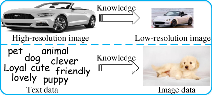
Figure 1. We aim to transfer knowledge between different feature spaces. Top row: transferring the knowledge from high-resolution images to low-resolution ones. Bottom row: transferring the knowledge from text data to image data.

To bridge between two heterogeneous domains, existing HDA works typically choose to project data from one domain to another (Xiao and Guo, 2015a; Kulis et al., 2011; Hoffman et al., 2013, 2014; Zhou et al., 2014; Tsai et al., 2016a, b), or find a domain-invariant subspace (Yao et al., 2015; Xiao and Guo, 2015b; Shi et al., 2010; Wang and Mahadevan, 2011; Duan et al., 2012; Li et al., 2014; Hsieh et al., 2016). On one hand, projections are learned in (Duan et al., 2012; Li et al., 2014; Hoffman et al., 2013, 2014) by performing the classifier adaptation strategy (i.e., training a domain-shared classifier with labeled cross-domain data). However, the type of methods does not explicitly minimize the distributional discrepancy across domains. On the other hand, another line of studies (Wang and Mahadevan, 2011; Tsai et al., 2016a) only considers the distribution matching strategy (i.e., reducing the distributional divergency between domains), but ignores the classifier adaptation one. Thus, this kind of methods does not directly align the discriminative directions of domains. Moreover, several works (Hsieh et al., 2016; Tsai et al., 2016b) derive the projections by iteratively performing the classifier adaptation and distribution matching. However, their performance is not stable since the iterative combination is a bit heuristic. In addition, they use trained classifier to assign each unlabeled target data to only one class that may be incorrect during the distribution matching, which is risky to negative transfer. Although Xiao and Guo (Xiao and Guo, 2015b) jointly consider the classifier adaptation and distribution matching in a unified framework, it does not further reduce the divergence between conditional distributions, which may be more important to the classification performance than aligning the marginal distributions. Note that all the above methods are shallow learning models that cannot learn more powerful feature representations. Although many deep learning models (Long et al., 2015, 2017, 2018; Bousmalis et al., 2016; Ding et al., 2018b) are developed for domain adaptation, they cannot be directly applied to solve the HDA problem. Only few works (Shu et al., 2015; Chen et al., 2016) solve the HDA problem by utilizing deep learning models. However, (Shu et al., 2015) requires the co-occurrence cross-domain data and (Chen et al., 2016) does not consider minimizing the distributional divergency across domains.

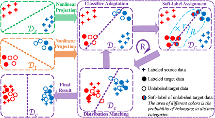
Figure 2. An illustrative example of STN. Here, $\mathcal{D}_{s}$, $\mathcal{D}_{t}$, and $\mathcal{D}_{c}$ denote the source domain (in green), the target domain (in orange), and the common subspace (in purple), respectively. $\left.r\middle/R\right.$ is the coefficient of the soft-label strategy to adaptively increase its importance, where $R$ is the total number of iterations and $r$ is the index of current iteration. Three key strategies are designed in STN for learning a domain-invariant $\mathcal{D}_{c}$. The classifier adaptation strategy aligns the discriminative directions of domains. The soft-label strategy avoids the hard assignment of each unlabeled target data to only one class that may be incorrect. The distribution matching strategy reduces the distributional divergence.

To overcome the limitations of the above methods, we propose a Soft Transfer Network (STN) for solving the HDA problem. The core rationale is depicted in Figure 2. In STN, we first project both the source and target data into a common subspace by using multiple nonlinear transformations. Then, a domain-invariant subspace is learned by jointly performing three key strategies: classifier adaptation, soft-label assignment, and distribution matching. The first stategy trains a domain-shared classifier with projected labeled source and target data by aligning the discriminative directions of domains. The second one assigns the soft-label (i.e., a probability distribution over all the categories) to each unlabeled target data, which prevents the hard assignment of each unlabeled target data to only one class that may be incorrect. In addition, we observe that the soft-labels will be more and more accurate as more iterations are executed. Thus, an adaptive coefficient is used to gradually increase the importance of the soft-labels. The last one matches both the marginal and conditional distributions between domains. Finally, we obtain a domain-shared classifier and a domain-invariant subspace for categorizing unlabeled target data.

The major contributions of this paper are three-fold. (1) To the best of our knowledge, there is no existing work that utilizes the soft-label strategy of unlabeled target data to address the HDA problem. (2) We propose a STN to learn a domain-shared classifier and a domain-invariant subspace in an end-to-end manner. (3) Extensive experimental results are presented on the transfer tasks of image-to-image, text-to-image, and text-to-text to verify the effectiveness of the proposed STN.

2. Related Work

As aforementioned, existing HDA models either project data from one domain to the other or derive a domain-invariant subspace. Accordingly, they can be grouped into two categories, namely asymmetric transformation method and symmetric transformation method.

Asymmetric transformation method. Kulis et al. (Kulis et al., 2011) present an Asymmetric Regularized Cross-domain Transformation (ARC-t) to project data from one domain to the other by learning an asymmetric nonlinear transformation. Zhou et al. (Zhou et al., 2014) introduce a Sparse Heterogeneous Feature Representation (SHFR) to project the weights of classifiers in the source domain into the target one via a sparse transformation. Hoffman et al. (Hoffman et al., 2013, 2014) propose a Max-Margin Domain Transform (MMDT), which maps the target data into the source domain by training a domain-shared support vector machine. Similarly, Xiao and Guo (Xiao and Guo, 2015a) develop a Semi-Supervised Kernel Matching for Domain Adaptation (SSKMDA) to transform the target data to similar source data, where a domain-shared classifier is simultaneously trained. Tsai et al. (Tsai et al., 2016a) propose a Label and Structure-consistent Unilateral Projection (LS-UP) model. This method maps the source data into the target domain with the aim of reducing the distributional difference and preserving the structure of projected data. They also propose a Cross-Domain Landmark Selection (CDLS) (Tsai et al., 2016b), where the representative source and target data are identified while reducing the distributional divergence between domains. Very recently, a few HDA approaches are presented based on the theory of Optimal Transport (OT) (Villani, 2008). For example, Ye et al. (Ye et al., 2018) develop a Metric Transporation on HEterogeneous REpresentations (MAPHERE) approach, which jointly learns an asymmetric transformation and an optimal transportation. Yan et al. (Yan et al., 2018) propose a Semi-supervised entropic Gromov-Wasserstein (SGW) discrepancy to transport source data into the target domain. Although this method utilizes the supervision information to guide the learning of optimal transport, it does not consider unlabeled target data when matching the conditional distributions between domains.

Symmetric transformation method. Shi et al. (Shi et al., 2010) develop a Heterogeneous spectral MAPping (HeMAP) to learn a pair of projections based on spectral embeddings. Wang and Mahadevan (Wang and Mahadevan, 2011) propose a Domain Adaptation using Manifold Alignment (DAMA) to find projections by preserving both the topology of each domain and the discriminative structure. Duan et al. (Duan et al., 2012) put forward a Heterogeneous Feature Augmentation (HFA) approach. This method works by first augmenting the projected data with the original data features and then training a domain-shared support vector machine with the augmented features. Subsequently, HFA is generalized to a semi-supervised extension named SHFA (Li et al., 2014) for effectively leveraging unlabeled target data. Xiao and Guo (Xiao and Guo, 2015b) present a Subspace Co-Projection with ECOC (SCP-ECOC) for HDA to learn projections by both training a domain-shared classifier and reducing the discrepancy on marginal distributions. Yao et al. (Yao et al., 2015) develop a Semi-supervised Domain Adaptation with Subspace Learning (SDASL) to learn projections by simultaneously minimizing the classification error, preserving the locality information of the original data, and considering the manifold structure of the target domain. Hsieh et al. (Hsieh et al., 2016) introduce a Generalized Joint Distribution Adaptation (G-JDA) model. This method reduces the difference in both the marginal and conditional distributions between domains while learning projections. Yan et al. (Yan et al., 2017b) present a Discriminative Correlation Analysis (DCA) to jointly learn a discriminative correlation subspace and a target domain classifier. Recently, Li et al. (Li et al., 2018) put forward a Progressive Alignment (PA) approach. This method first learns a common subspace by dictionary-shared sparse coding, and then mitigates the distributional divergence between domains. Besides, some HDA methods are developed based on deep learning models. For instance, Shu et al. (Shu et al., 2015) propose a weakly-shared Deep Transfer Network (DTN) to address the learning of heterogeneous cross-domain data, but it requires the co-occurrence cross-domain data. Recently, Chen et al. (Chen et al., 2016) put forward a Transfer Neural Trees (TNT) for HDA, which jointly addresses cross-domain feature projection, adaptation, and recognition in an end-to-end network. However, TNT does not explicitly minimize the distributional divergence across domains.

Moreover, our work is related to a few homogeneous DA studies that utilize the pseudo-label strategy of unlabeled target data. Specifically, Long et al. (Long et al., 2013) propose a Joint Distribution Adaptation (JDA) to align both the marginal and conditional distributions between domains. As a follow-up, in (Long et al., 2014) they further develop a Adaptation Regularization based Transfer Learning (ARTL) framework. This method works by simultaneously minimizing the structural risk, reducing the distributional divergence, and acquiring the manifold information. Yan et al. (Yan et al., 2017a) introduce a weighted MMD to mitigate the effect of class weight bias, and further propose a Weighted Domain Adaptation Network (WDAN) to address the learning of homogeneous cross-domain data. Zhang et al. (Zhang et al., 2017) present a Joint Geometrical and Statistical Alignment (JGSA) to reduce both the distributional and geometrical divergence across domains. Wang et al. (Wang et al., 2018) propose a Manifold Embedded Distribution Alignment (MEDA) approach, which learns a domain-invariant classifier by both minimizing the structural risk and performing dynamic distribution alignment. Ding et al. (Ding et al., 2018a) put forward a Graph Adaptive Knowledge Transfer (GAKT) to jointly learn target labels and domain-invariant features. However, these methods either learn a feature transformation shared by cross-domain data (Long et al., 2013, 2014; Yan et al., 2017a; Wang et al., 2018), or learn two feature transformations with the same size to constrain the divergence between transformations (Zhang et al., 2017; Ding et al., 2018a), which thus cannot directly deal with the HDA problem.

Overall, our work belongs to the symmetric transformation method. Inspired by the above-mentioned studies, we propose to jointly learn a domain-shared classifier and a domain-invariant subspace in an end-to-end manner, which not only aligns the discriminative directions of domains but also reduces the distributional divergence between domains.

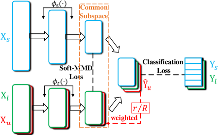
Figure 3. The architecture of the proposed STN, where $\{\mathbf{X}_{s},\mathbf{Y}_{s}\}$ (in blue) and $\{\mathbf{X}_{l},\mathbf{Y}_{l}\}$ (in green) are labeled source and target data, respectively, $\mathbf{X}_{u}$ (in red) is unlabeled target data, $\widehat{\mathbf{Y}}_{u}=f(\phi_{t}(\mathbf{X}_{u}))$ (in red) is the soft-label of $\mathbf{X}_{u}$, $\phi_{s}(\cdot)$ and $\phi_{t}(\cdot)$ are feature projection networks of the source and target domains, respectively. Our model consists of two losses: a classification loss for aligning the discriminative directions of domains, and a soft-MMD loss to reduce the distributional divergence across domains.

3. Soft Transfer Network

In this section, we present the proposed STN. We begin with the definitions and terminologies. The source domain is denoted by $\mathcal{D}_{s}=\{(\mathbf{x}^{s}_{i},y^{s}_{i})\}_{i=1}^{n_{s}}$, where $\mathbf{x}^{s}_{i}\in\mathbb{R}^{d_{s}}$ is the $i$-th source domain data with $d_{s}$-dimensional features, and $y^{s}_{i}\in\mathcal{Y}=\{1,2,\cdots,C\}$ is its associated class label with $C$ as the number of classes. Similarly, let $\mathcal{D}_{t}=\mathcal{D}_{l}\cup\mathcal{D}_{u}=\{(\mathbf{x}^{l}_{i},y^{l}_{i})\}_{i=1}^{n_{l}}\cup\{\mathbf{x}^{u}_{i}\}_{i=1}^{n_{u}}$ be the target domain, where $\mathbf{x}^{l}_{i}$ $(\mathbf{x}^{u}_{i})\in\mathbb{R}^{d_{t}}$ is the $i$-th labeled (unlabeled) target domain data with $d_{t}$-dimensional features, and $y^{l}_{i}\in\mathcal{Y}$ is the corresponding class label. Note that in the HDA problem, we have $d_{s}\not=d_{t}$, $n_{s}\gg n_{l}$, and $n_{u}\gg n_{l}$. The goal is to design a heterogeneous transfer network for predicting the labels of unlabeled target domain data in $\mathcal{D}_{u}$.

For simplicity of presentation, we denote by $\mathbf{X}_{s}=[\mathbf{x}_{1}^{s},\cdots,\mathbf{x}_{n_{s}}^{s}]^{\mathrm{T}}\in\mathbb{R}^{n_{s}\times d_{s}}$ the data matrix in $\mathcal{D}_{s}$ and by $\mathbf{Y}_{s}$ = $[\mathbf{g}_{y_{1}^{s}},\cdots,\mathbf{g}_{y_{n_{s}}^{s}}]^{\mathrm{T}}\in\mathbb{R}^{n_{s}\times C}$ the corresponding label matrix, where $\mathbf{g}_{y}\in\mathbb{R}^{C}$ denotes a one-hot vector with the $y$-th element being one. Analogously, let $\mathbf{X}_{l}=[\mathbf{x}_{1}^{l},\cdots,\mathbf{x}_{n_{l}}^{l}]^{\mathrm{T}}\in\mathbb{R}^{n_{l}\times d_{t}}$ be the data matrix in $\mathcal{D}_{l}$ with an associated label matrix $\mathbf{Y}_{l}=[\mathbf{g}_{y_{1}^{l}},\cdots,\mathbf{g}_{y_{n_{l}}^{l}}]^{\mathrm{T}}\in\mathbb{R}^{n_{l}\times C}$ and $\mathbf{X}_{u}=[\mathbf{x}_{1}^{u},\cdots,\mathbf{x}_{n_{u}}^{u}]^{\mathrm{T}}\in\mathbb{R}^{n_{u}\times d_{t}}$ be the data matrix in $\mathcal{D}_{u}$. We also denote by $\mathbf{X}_{t}=\left[\mathbf{X}_{l};\mathbf{X}_{u}\right]\in\mathbb{R}^{n_{t}\times d_{t}}$ the data matrix in $\mathcal{D}_{t}$, where $n_{t}=n_{l}+n_{u}$ is the total number of the target domain data.

The key challenge of HDA arises in that the feature spaces of the source and target domains are different. Thus, we cannot directly transfer knowledge from the source domain to the target one. To approach this problem, we first assume there is a common subspace with the dimensionality $d$, and then build two projection networks $\phi_{s}(\cdot):\mathbb{R}^{d_{s}}\rightarrow\mathbb{R}^{d}$ and $\phi_{t}(\cdot):\mathbb{R}^{d_{t}}\rightarrow\mathbb{R}^{d}$, which are used to transform source and target data into the subspace, respectively. We aim to find the optimal projection networks $\phi_{s}(\cdot)$ and $\phi_{t}(\cdot)$, which can form a domain-invariant subspace and lead to an effective transfer strategy. As depicted in Figure 3, we achieve this by optimizing an objective function with two components: a classification loss for aligning the discriminative directions of domains, and a Soft-MMD loss to reduce the distributional divergence across domains. The details of each component will be described in the following sections.

3.1. Classification Loss

We apply the classification loss to train a domain-shared classifier $f(\cdot)$ with projected labeled source and target data. It can be used to align the discriminative directions of domains. Further, we propose to jointly learn $f(\cdot)$, $\phi_{s}(\cdot)$, and $\phi_{t}(\cdot)$ under the Structural Risk Minimization (SRM) framework (Vapnik, 1998), and formulate the classification loss as

(1) $$\small\mathcal{L}_{c}\big{[}\mathbf{Y}_{a},f(\mathbf{X}_{a})\big{]}=\frac{1}{n_{s}+n_{l}}\mathcal{L}\big{[}\mathbf{Y}_{a},f(\mathbf{X}_{a})\big{]}+\tau\big{(}\left\|\phi_{s}\right\|^{2}+\left\|\phi_{t}\right\|^{2}+\left\|f\right\|^{2}\big{)},$$

where $\mathbf{X}_{a}=\big{[}\phi_{s}(\mathbf{X}_{s});\phi_{t}(\mathbf{X}_{l})\big{]}\in\mathbb{R}^{(n_{s}+n_{l})\times d}$ denotes projected labeled data matrix in two domains, $\mathbf{Y}_{a}=\big{[}\mathbf{Y}_{s};\mathbf{Y}_{l}\big{]}\in\mathbb{R}^{(n_{s}+n_{l})\times C}$ is the associated label matrix, $\mathcal{L}[\cdot,\cdot]$ is the cross-entropy function, $f(\cdot)$ is the softmax function, and $\tau$ is a positive regularization parameter. According to the SRM principle, the domain-shared classifier $f(\cdot)$ can accurately predict unknown target data by minimizing Eq. (1), given the domain-invariant subspace.

3.2. Soft-MMD Loss

As mentioned above, we expect to discover a domain-invariant subspace by enforcing the discriminative structure of the source domain to be consistent with that of the target domain. If there are sufficient labeled data in both domains, we can make it by only minimizing Eq. (1). However, the labeled target data is very scarce, which is not enough to identify a domain-invariant subspace. To eliminate this problem, we design a Soft Maximum Mean Discrepancy (Soft-MMD) loss, which can be applied to match both the marginal and conditional distributions between domains. As a result, the Soft-MMD loss is formulated as

(2) $$\small\mathcal{L}_{s}\big{[}\phi_{s}(\mathbf{X}_{s}),\phi_{t}(\mathbf{X}_{t})\big{]}=\mathcal{Q}_{m}\big{[}\phi_{s}(\mathbf{X}_{s}),\phi_{t}(\mathbf{X}_{t})\big{]}+\mathcal{Q}_{c}\big{[}\phi_{s}(\mathbf{X}_{s}),\phi_{t}(\mathbf{X}_{t})\big{]},$$

where $\mathcal{Q}_{m}[\cdot,\cdot]$ acts as the divergence between marginal distributions of projected cross-domain data, and $\mathcal{Q}_{c}[\cdot,\cdot]$ stands for that between conditional distributions.

We first detail how to formulate $\mathcal{Q}_{m}[\cdot,\cdot]$. The empirical Maximum Mean Discrepancy (MMD) (Gretton et al., 2007) has been proven to be a powerful tool for measuring the divergency between marginal distributions. Its exact idea is to calculate the distance between the centroids of both the source and target data, and then uses the distance to model the discrepance on marginal distributions. Thus, we define $\mathcal{Q}_{m}[\cdot,\cdot]$ as

(3) $$\small\mathcal{Q}_{m}\big{[}\phi_{s}(\mathbf{X}_{s}),\phi_{t}(\mathbf{X}_{t})\big{]}=\left\|\frac{1}{n_{s}}\sum_{i=1}^{n_{s}}\widetilde{\mathbf{x}}_{i}^{s}-\frac{1}{n_{t}}\sum_{i=1}^{n_{t}}\widetilde{\mathbf{x}}_{i}^{t}\right\|^{2},$$

where $\widetilde{\mathbf{x}}_{i}^{s}$ and $\widetilde{\mathbf{x}}_{i}^{t}$ are the $i$-th projected source and target data, respectively.

Next, we describe how to design $\mathcal{Q}_{c}[\cdot,\cdot]$. Since directly modelling the conditional distribution (i.e., $\mathcal{P}(Y|X)$) is difficult, we turn to explore the class-conditional distribution (i.e., $\mathcal{P}(X|Y)$) instead (Long et al., 2013; Tsai et al., 2016b; Hsieh et al., 2016), and apply the divergency between class-conditional distributions to approximate that between conditional distributions. Hence, the divergence on conditional distributions can be approximated by calculating the sum of the distance between centroids of both the source and target data in each category. However, a large amount of target data has no label information. To make full use of unlabeled target data, (Long et al., 2013) first proposes to use the hard-label strategy of unlabeled target data, which can be performed by applying a base classifier trained on labeled cross-domain data to unlabeled target data. Although this srategy may boost the adaptation performance, we note that it enforces each unlabeled target data to be assigned the class with the highest predicted probability, which may have two potential risks: (i) some unlabeled target data are aligned to incorrect class centroids since their hard-labels may be incorrect; and (ii) because of issue (i), negative transfer may occur. To alleviate these risks, we propose to adopt the soft-label strategy of unlabeled target data instead, which avoids the hard assignment of each unlabeled target data to only one class that may be incorrect. Concretely, the soft-label of the $i$-th projected unlabeled target data $\mathbf{\widetilde{x}}_{i}^{u}$, i.e., $\widehat{\mathbf{y}}_{i}^{u}=f(\phi_{t}(\mathbf{x}_{i}^{u}))$, is a $C$-dimensional vector, where the $k$-th element $\widehat{y}_{k,i}^{u}$ indicates the probability of $\mathbf{\widetilde{x}}_{i}^{u}$ belonging to class $k$. We use $\widehat{y}_{k,i}^{u}$ as the weight of $\mathbf{\widetilde{x}}_{i}^{u}$ to calculate the centroid of the $k$-th class in the target domain. Accordingly, a preliminary divergence between class-conditional distributions in the two domains is designed as

(4) $$\small\mathcal{Q}_{c}^{{}^{\prime}}\big{[}\phi_{s}(\mathbf{X}_{s}),\phi_{t}(\mathbf{X}_{t})\big{]}=\sum_{k=1}^{C}\left\|\frac{1}{n_{s}^{k}}\sum_{i=1}^{n_{s}^{k}}\mathbf{\widetilde{x}}_{k,i}^{s}-\frac{\sum_{i=1}^{n_{l}^{k}}\widetilde{\mathbf{x}}_{k,i}^{l}+\sum_{i=1}^{n_{u}}\widehat{y}_{k,i}^{u}\widetilde{\mathbf{x}}_{i}^{u}}{n_{l}^{k}+\sum_{i=1}^{n_{u}}\widehat{y}_{k,i}^{u}}\right\|^{2},$$

where $\mathbf{\widetilde{x}}_{k,i}^{s}$ and $\mathbf{\widetilde{x}}_{k,i}^{l}$ are the $i$-th projected labeled source and target data of class $k$, respectively, and $n^{k}_{s}$, $n^{k}_{l}$ are the number of labeled source and target data of class $k$, respectively. If $\widehat{y}_{k,i}^{u}$ adopts the hard-label strategy as in (Long et al., 2013), then Eq. (4) reduces to the hard-label approach (Long et al., 2013). Therefore, the proposed soft-label approach is a generalization of the hard-label approach (Long et al., 2013).

Besides the soft-label strategy introduced in Eq. (4), we present another iterative weighting mechanism to further circumvent the risks mentioned above. We observe that the performance of $f(\cdot)$ gradually improves as the number of iterations increases. Thus, the value of $\widehat{y}_{k,i}^{u}$ will become more and more precise and reliable as more iterations are performed. As a result, we itroduce an adaptive coefficient to gradually increase the importance of $\widehat{y}_{k,i}^{u}$ during adaptation, and based on $\mathcal{Q}_{c}^{{}^{\prime}}[\cdot,\cdot]$ formulate $\mathcal{Q}_{c}[\cdot,\cdot]$ as

(5) $$\small\mathcal{Q}_{c}\big{[}\phi_{s}(\mathbf{X}_{s}),\phi_{t}(\mathbf{X}_{t})\big{]}=\sum_{k=1}^{C}\left\|\frac{1}{n_{s}^{k}}\sum_{i=1}^{n_{s}^{k}}\mathbf{\widetilde{x}}_{k,i}^{s}-\frac{\sum_{i=1}^{n_{l}^{k}}\widetilde{\mathbf{x}}_{k,i}^{l}+\sum_{i=1}^{n_{u}}\alpha_{i}^{(r)}\widetilde{\mathbf{x}}_{i}^{u}}{n_{l}^{k}+\sum_{i=1}^{n_{u}}\alpha_{i}^{(r)}}\right\|^{2},$$

where $\alpha_{i}^{(r)}$ is defined by

(6) $$\small\alpha_{i}^{(r)}=\frac{r*\widehat{y}_{k,i}^{u}}{R},$$

which is used to adaptively increase the importance of $\widehat{y}_{k,i}^{u}$. Here, $R$ is the total number of iterations, and $r$ is the index of current iteration.

3.3. The Overall Objective of STN

In summary, to safely transfer knowledge across heterogeneous domains, the ideal model should be able to find the domain-shared classifier, i.e., optimal $f(\cdot)$, and the domain-invariant subspace, i.e, optimal $\phi_{s}(\cdot)$ and $\phi_{t}(\cdot)$. To this end, we integrate all of the components aforementioned into an end-to-end network, and obtain the overall objective function of STN:

(7) $$\small\min_{\phi_{s},\phi_{t},f}\mathcal{L}_{c}\big{[}\mathbf{Y}_{a},f(\mathbf{X}_{a})\big{]}+\beta\mathcal{L}_{s}\big{[}\phi_{s}(\mathbf{X}_{s}),\phi_{t}(\mathbf{X}_{t})\big{]},$$

where $\beta$ is a tradeoff parameter to balance the importance between $\mathcal{L}_{c}[\cdot,\cdot]$ and $\mathcal{L}_{s}[\cdot,\cdot]$. The proposed STN can jointly learn $f(\cdot)$, $\phi_{s}(\cdot)$, and $\phi_{t}(\cdot)$ in an end-to-end network by minimizing Eq. (7). Furthermore, STN adopts both the soft-label and the iterative weighting strategies to match the distributions. These are why STN can be expected to perform quite well as reported in the next section.

Table 1. Classification accuracies (%) of all the methods on all the image-to-image transfer tasks.

$\mathcal{D}_{s}\rightarrow\mathcal{D}_{t}$	SVMt	NNt	MMDT	SHFA	G-JDA	CDLS	SGW	TNT	STN
C$\rightarrow$A	89.13$\pm$0.39	89.6$\pm$0.33	87.06$\pm$0.47	85.49$\pm$0.51	92.49$\pm$0.12	86.34$\pm$0.74	89.03$\pm$0.37	92.35$\pm$0.17	93.03$\pm$0.16
W$\rightarrow$A			87$\pm$0.47	88.83$\pm$0.45	92.28$\pm$0.15	87.51$\pm$0.44	89.02$\pm$0.37	92.99$\pm$0.14	93.11$\pm$0.16
A$\rightarrow$C	79.64$\pm$0.46	81.03$\pm$0.5	75.62$\pm$0.57	71.16$\pm$0.73	86.6$\pm$0.17	78.73$\pm$0.49	79.88$\pm$0.53	85.79$\pm$0.42	88.21$\pm$0.16
W$\rightarrow$C			75.44$\pm$0.59	79.66$\pm$0.52	84.82$\pm$0.38	77.3$\pm$0.71	79.85$\pm$0.53	86.28$\pm$0.51	87.22$\pm$0.45
A$\rightarrow$W	89.34$\pm$0.94	91.13$\pm$0.73	89.28$\pm$0.77	88.11$\pm$1.01	94.09$\pm$0.67	91.57$\pm$0.81	90.26$\pm$0.84	91.26$\pm$0.72	96.68$\pm$0.43
C$\rightarrow$W			89.11$\pm$0.76	89.47$\pm$0.9	92.64$\pm$0.54	88.6$\pm$0.8	90.26$\pm$0.84	92.98$\pm$0.75	96.38$\pm$0.38
A$\rightarrow$D	92.6$\pm$0.71	92.99$\pm$0.63	91.65$\pm$0.83	95.16$\pm$0.36	90.67$\pm$0.65	94.45$\pm$0.59	93.43$\pm$0.67	92.04$\pm$0.76	96.42$\pm$0.43
C$\rightarrow$D			91.46$\pm$0.85	94.25$\pm$0.5	88.62$\pm$0.76	90.43$\pm$0.79	93.43$\pm$0.67	92.67$\pm$0.8	96.06$\pm$0.5
W$\rightarrow$D			91.77$\pm$0.83	95.31$\pm$0.63	95.87$\pm$0.41	92.72$\pm$0.75	93.43$\pm$0.67	94.09$\pm$0.88	96.38$\pm$0.57
Avg.	87.68$\pm$0.63	88.69$\pm$0.55	86.49$\pm$0.68	87.49$\pm$0.62	90.9$\pm$0.43	87.52$\pm$0.68	88.73$\pm$0.61	91.17$\pm$0.44	93.72$\pm$0.36

Table 2. Classification accuracies (%) of all the methods on the text-to-image transfer task.

$\mathcal{D}_{s}\rightarrow\mathcal{D}_{t}$	SVMt	NNt	MMDT	SHFA	G-JDA	CDLS	SGW	TNT	STN
text$\rightarrow$image	66.85$\pm$0.96	67.68$\pm$0.8	53.21$\pm$0.69	64.06$\pm$0.61	75.76$\pm$0.65	70.96$\pm$0.83	68.01$\pm$0.8	77.71$\pm$0.57	78.46$\pm$0.58

3.4. Comparison with Existing Studies

We now compare the proposed STN with some existing studies. To our knowledge, the methods related to STN include MMDT (Hoffman et al., 2013, 2014), HFA (Duan et al., 2012), SHFA (Li et al., 2014), G-JDA (Hsieh et al., 2016), CDLS (Tsai et al., 2016b), SGW (Yan et al., 2018), SCP-ECOC (Xiao and Guo, 2015b), JDA (Long et al., 2013), JGSA (Zhang et al., 2017), ARTL (Long et al., 2014), MEDA (Wang et al., 2018), WDAN (Yan et al., 2017a), and GAKT (Ding et al., 2018a). Among these methods, the first seven ones belong to heterogeneous DA techniques, while the last six methods are homogeneous DA ones. However, our work substantially distinguishes from them in the following aspects:

• Comparison with heterogeneous DA studies. (1) MMDT, HFA, and SHFA only consider the classifier adaptation. (2) G-JDA, CDLS, and SGW iteratively perform the classifier adaptation and distribution matching. Moreover, G-JDA and CDLS adopt the hard-label strategy to align the conditional distributions, and SGW does not take it into account. (3) SCP-ECOC only matches the marginal distributions.

• Comparison with homogeneous DA studies. (1) JDA and JGSA take the classifier adaptation and distribution matching as two independent tasks. (2) JDA, JGSA, ARTL, and MEDA utilize the hard-label strategy to reduce the conditional distribution divergence. (3) WDAN estimates the weights of the source data based on the hard-label strategy. (4) GAKT adopts the graph Laplacian regularization to perform the soft-label strategy and neglects the iterative weighting mechanism.

4. Experiments

In this section, we empirically evaluate the proposed STN on the transfer tasks of image-to-image, text-to-image, and text-to-text.

4.1. Datasets and Settings

The image-to-image transfer task is performed on the Office+Cal-tech-256 dataset (Saenko et al., 2010; Griffin et al., 2007). The former comprises 4,652 images with 31 categories collected from three distinct domains: Amazon (A), Webcam (W), and DSLR (D), and the latter includes 30,607 images of 256 objects from Caltech-256 (C). Following the settings in (Hsieh et al., 2016; Tsai et al., 2016b; Chen et al., 2016), we choose 10 overlapping categories of these two datasets to construct the Office+Caltech-256 dataset. Furthermore, we adopt two different feature representations for this type of task: 800-dimension $SURF$ (Bay et al., 2006) and 4096-dimension $DeCAF_{6}$ (Donahue et al., 2014). Some sample images of the category of bike are shown in Figure 4.

The text-to-image transfer task is conducted on the NUS-WIDE+ImageNet dataset (Chua et al., 2009; Deng et al., 2009). The former consists of 269,648 images and the associated tags from Flickr, while the latter includes 5,247 synsets and 3.2 million images. We use the tag information of NUS-WIDE (N) and the image data of ImageNet (I) as the domains for text and image, respectively. Following (Chen et al., 2016), we select 8 shared categories of the two datasets to generate the NUS-WIDE+ImageNet dataset. Moreover, we follow (Chen et al. 2016) to extract the 4-th hidden layer from a 5-layer neural network as the 64-dimensional feature representation for text data, and to extract $DeCAF_{6}$ feature as the 4096-dimensional feature representation for image data.

The text-to-text transfer task is executed on the Multilingual Reuters Collection dataset (Amini et al., 2009). This dataset contains about 11,000 articles from 6 categories written in five different languages: English (E), French (F), German (G), Italian (I), and Spanish (S). We follow (Duan et al., 2012; Li et al., 2014; Hsieh et al., 2016; Tsai et al., 2016b) to represent all the articles by BOW with TF-IDF features, and then to reduce the dimensions of features by performing PCA with $60\%$ energy preserved. The final dimensions w.r.t. E, F, G, I, and S are 1,131, 1,230, 1,417, 1,041, and 807, respectively.

We implement the proposed STN based on the TensorFlow framework (Abadi et al., 2016). For the sake of fair comparison, we fix the parameter settings of STN for all the tasks. Both $\phi_{s}(\cdot)$ and $\phi_{t}(\cdot)$ are two-layer neural networks, which adopt Leaky ReLU (Maas et al., 2013) as the activation function. We use the Adam optimizer (Kingma and Ba, 2015) with a learning rate of 0.001, and empirically set hyper-parameters $\beta=0.001,\tau=0.001$. In addition, the dimension of the common subspace $d$ and the number of iterations $R$ are set to 256 and 300, respectively.

Figure 4. Sample images of the bike category from the Office+Caltech-256 dataset.

4.2. Evaluations

We evaluate the proposed STN against eight state-of-the-art supervised learning and HDA methods, i.e., SVMt, NNt, MMDT (Hoffman et al., 2013, 2014), SHFA (Li et al., 2014), G-JDA (Hsieh et al., 2016), CDLS (Tsai et al., 2016b), SGW (Yan et al., 2018), and TNT (Chen et al., 2016). Among these methods, SVMt and NNt train a support vector machine and a neural network with only the labeled target data, respectively. MMDT, SHFA, G-JDA, CDLS, and SGW are the shallow HDA methods, while TNT is the deep HDA one. Furthermore, we note that SHFA, G-JDA, CDLS, SGW, and TNT are semi-supervised HDA methods, which learn from both labeled and unlabeled cross-domain data. As stated in Section 2, homogeneous DA methods cannot directly apply to the HDA problem, thus we do not include them in the comparison. Following (Li et al., 2014; Hsieh et al., 2016; Chen et al., 2016; Tsai et al., 2016b; Yan et al., 2018), we use the classification accuracy as the evaluation metric.

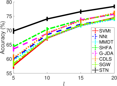
(a) E$\rightarrow$S

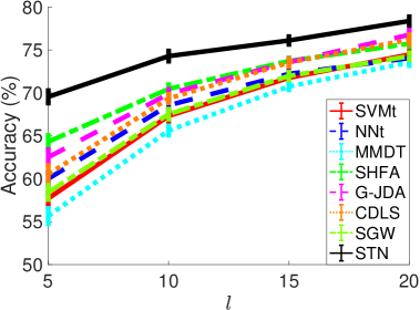
(b) F$\rightarrow$S

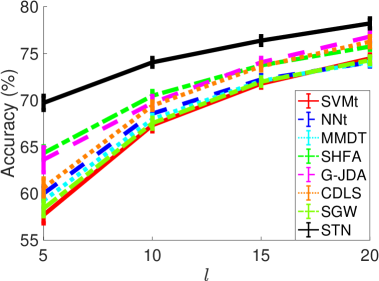
(c) G$\rightarrow$S

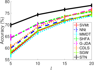
(d) I$\rightarrow$S

Figure 5. Classification accuracies (%) of all the methods with different numbers of labeled target data per category (i.e., $l=5,10,15,20$) on all the text-to-text transfer tasks.

Image-to-image transfer: We first perform the task of image-to-image transfer on the Office+Caltech-256 dataset. In this kind of task, the source and target data are drawn from not only different feature representations but also distinct domains. As for the source domain, we take images in $SURF$ features and utilize all images as the labeled data. For the target domain, we represent images with $DeCAF_{6}$ features and randomly sample 3 images per class as the labeled data. The remaining images in the target domain are used as the testbed. Moreover, D is only viewed as the target domain due to the limited amount of images. Table 1 presents the average classification accuracies of 20 random trials.

From the results, we can make several insightful observations. (1) The proposed STN consistently achieves the highest accuracies on all the tasks. The average classification accuracy of STN is 93.72%, which makes the improvement over the best supervised learning method, i.e., NNt, and the best HDA method, i.e., TNT, by 5.03% and 2.55%, respectively. These results clearly demonstrate the superiority of STN. (2) STN performs significantly better than MMDT and SHFA. The reason is that they only consider the classifier adaptation strategy but neglect the distribution matching strategy which can reduce the distributional divergence across domains. Although G-JDA and CDLS combine both strategies for HDA, their performance is still worse than STN. One reason is because they iteratively perform the strategies of classifier adaptation and distribution matching. The iterative combination is a bit heuristic and may lead to unstable performance. Another important reason is that they use the hard-label strategy of unlabeled target data during the distribution matching. The hard-labels may be not correct, which may result in limited performance improvement and negative transfer. The performance of SGW is worse than STN. An important reason is that SGW does not utilize unlabeled target data to align the conditional distributions between domains. STN yields better performance than TNT with one reason that TNT does not explicitly minimize the distributional discrepancy between domains. (3) MMDT and SHFA do not always outperform the supervised learning method, i.e., SVMt. One possible explanation is that the distributional divergence across domains may be large. Although they both train a domain-shared classifier to align the discriminative directions of domains, they do not minimize the distributional difference very well due to the limited amount of the labeled target data. Thus, it is risky to overfit the target data that result in negative transfer. In addition, SHFA exceeds MMDT with one major reason that the former utilizes the unlabeled target data while the latter does not. (4) G-JDA, CDLS, and SGW are better or comparable than SVMt. They iteratively perform the strategies of classifier adaptation and distribution matching, which confirms that these strategies are both meaningful and useful. In addition, we note that CDLS achieves worse performance than G-JDA. A possible explanation is that the instance weighting scheme used in CDLS is not always beneficial and may hurt the performance. (5) STN and TNT perform better than all the other methods, which verifies deep models are effective for addressing the HDA problem in the image domain.

Text-to-image transfer: We then conduct the text-to-image transfer task on the NUS-WIDE+ImageNet dataset. It is very hard because there is no co-occurrence text and image data for learning. According to (Chen et al., 2016), we treat the text (i.e., N) and image (i.e., I) datasets as the source and target domains, respectively. For the source domain, we choose 100 texts per category as the labeled data. As for the target domain, we randomly sample 3 images as the labeld data from each class, and the rest images are considered as the testbed. Table 2 shows the average classification accuracies in 20 random trials.

From the results, we can make the following important observations. (1) The proposed STN achieves the best performance on this task. The classification accuracy of STN is 78.46%, which outperforms the best supervised learning method, i.e., NNt, and the best HDA method, i.e., TNT, by 10.78% and 0.75%, respectively. These results further corroborate the effectiveness of STN. (2) Both STN and TNT significantly exceed the other methods, which again verifies deep networks is helpful for learning heterogeneous cross-domain data. (3) The performance of MMDT is quite poor. This observation is consistent with (Chen et al., 2016) with one possible reason that the distributional divergence between domains may be very large since the source domain is textual while the target one is visual. (4) We have the same observation as the image-to-image transfer task that SHFA and G-JDA are better than MMDT and CDLS, respectively.

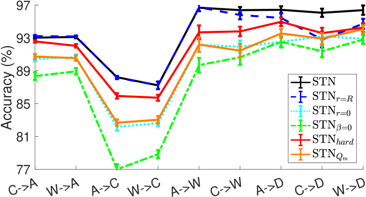
Figure 6. Performance comparison of STN and its variants on all the image-to-image transfer tasks. Here, STN_r=R removes the iterative weighting mechanism, STN_r=0 ignores the unlabeled target data, STN_β=0 ablates the soft-MMD loss, STN_hard adopts the hard-label strategy of unlabeled target data, and STN${}_{Q_{m}}$ neglects the divergence between conditional distributions.

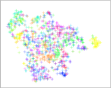
(a) C with $SURF$

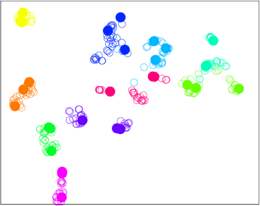
(b) W with $DeCAF_{6}$

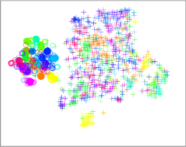
(c) MMDT

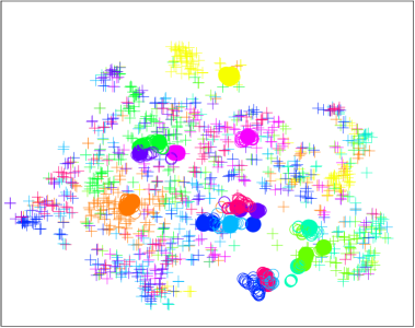
(d) G-JDA

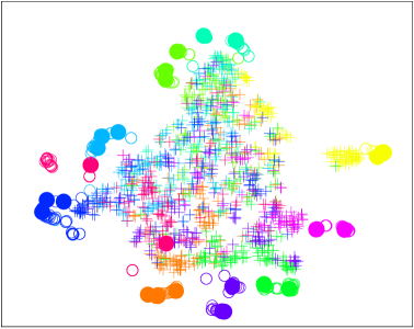
(e) CDLS

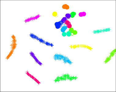
(f) SGW

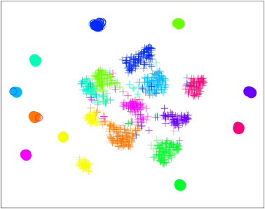
(g) TNT

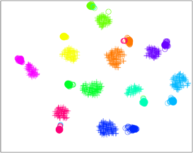
(h) STN

Figure 7. The t-SNE visualization on the C$\rightarrow$W task. Here, (a) and (b) are the original feature representations of $SURF$ and $DeCAF_{6}$, respectively. (c), (d), (e), (f), (g), and (h) are the learned feature representations of MMDT, G-JDA, CDLS, SGW, TNT, and STN, respectively.

Text-to-text transfer: We now execute the text-to-text transfer task on the Multilingual Reuters Collection dataset. In this type of task, we regard articles in distinct languages as data in different domains. According to the settings in (Duan et al., 2012; Li et al., 2014; Hsieh et al., 2016; Tsai et al., 2016b), we consider E, F, G and I as the source domains, and S as the target one. For the source domain, we randomly pick up 100 articles per category as the labeled data. As for the target domain, we randomly select $l$ (i.e., $l=5,10,15,20$) and 500 articles per class as the labeled and unlabeled data, respectively. We explore how the number of labeled target data per category $l$ affects the performance and plot the average classification accuracies of 20 random trials in Figure 5. We do not report the results of TNT as they are much worse than the other methods (we note that the original paper of TNT also does not report the results on this type of task, please refer to (Chen et al., 2016) for details).

From the results, we have several interesting observations. (1) The performance of all the methods are boosted with the increase of the number of labeled target data. This observation is intuitive and reasonable. (2) The proposed STN substantially outperforms all the baseline methods on all the tasks. In particular, the average classification accuracy of STN with 5 labeled target data on all the tasks is 69.75%, which outperforms the best supervised learning method, i.e., NNt, and the best HDA method, i.e., SHFA, by 9.75% and 5.42%, respectively. These results verify the effectiveness of STN again. (3) All the HDA methods can yield comparable or better performance than the supervised learning method, i.e., SVMt, which implies that these methods can produce positive transfer on all the text-to-text transfer tasks. (4) SHFA and G-JDA outperform MMDT and CDLS, respectively. We have the same observation as that on the image-to-image and text-to-image transfer tasks.

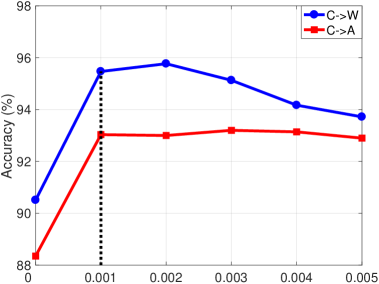
(a) $\beta$

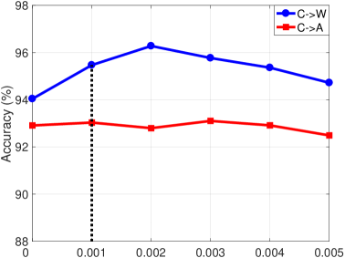
(b) $\tau$

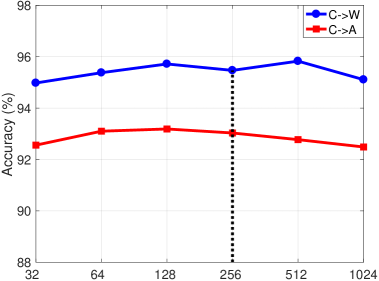
(c) $d$

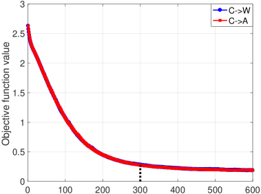
(d) $R$

Figure 8. Parameter sensitivity and convergence analysis on the transfer tasks of C$\rightarrow$W and C$\rightarrow$A.

4.3. Analysis

Variants Evaluation: To go deeper with the efficacy of the iterative weighting mechanism, the distribution matching strategy, and the soft-label strategy, we evaluate several variants of STN: (1) STN_r=R, which removes the iterative weighting mechanism by setting $r=R$ in Eq. (6); (2) STN_r=0, which ignores the unlabeled target data by setting $r=0$ in Eq. (6); (3) STN_β=0, which ablates the soft-MMD loss by setting $\beta=0$ in Eq. (7); (4) STN_hard, which adopts the hard-label strategy of unlabeled target data and iteratively performs the hard-label assignment and objective optimizing in an end-to-end network; and (5) STN${}_{Q_{m}}$, which neglects the divergence on the conditional distributions by ablating $Q_{c}$ in Eq. (2). We use the same experimental setting as above and plot the average classification accuracies on all the image-to-image transfer tasks in Figure 6. The results reveal several insightful observations. (1) As expected, STN delivers the best performance on all the tasks. (2) STN_r=R is worse than STN, which suggests that the iterative weighting mechanism is useful to further improve the performance. STN_hard is worse than STN and STN_r=R, which implies that the soft-label strategy is more suitable to match the conditional distributions between domains than the hard-label. STN_r=0 is worse than STN, STN_r=R, and STN_hard, which indicates that using the unlabeled target data can further improve the performance without resulting in negative transfer on these tasks. STN${}_{Q_{m}}$ is worse than STN, STN_r=R, and STN_hard, which indicates that aligning the conditional distributions is useful. STN${}_{Q_{m}}$ is similar to STN_r=0, which implies that using the unlabeled target data is important for reducing the divergence on conditional distributions. STN_β=0 yields the worst performance, which suggests that the distribution matching strategy is necessary and helpful for transferring knowledge across heterogeneous domains.

Feature Visualization: We use the t-SNE technique (van der Maaten, 2014) to visualize the learned features of all the methods on the task of C$\rightarrow$W except SHFA because it does not explicitly learn the feature projection matrices (please refer to (Li et al., 2014) for details). We plot the visualization results in Figure 7. The results offer several interesting observations. (1) Comparing Figure 7(a) with Figure 7(b), we can see that the discriminative ability of $DeCAF_{6}$ is better than $SURF$, which is reasonable as $DeCAF_{6}$ is the deep feature. (2) For MMDT, G-JDA, CDLS, SGW, and TNT, we can find that they do not align the distributions between domains very well, which explains their poor performance on this task. (3) The proposed STN matches the distributions between domains very well, which indicates that STN is powerful for transferring knowledge across heterogeneous domains.

Parameter Sensitivity and Convergence: We conduct experiments to analyze the parameter sensitivity and the convergence of STN on the transfer tasks of C$\rightarrow$W and C$\rightarrow$A. Figures 8(a)-8(c) show the accuracy w.r.t. $\beta$, $\tau$, and $d$, respectively. We can observe that the default values ($\beta=0.001,\tau=0.001,d=256$) can achieve high accuracies. It is worth noting that STN yields the state-of-the-art performance on all the tasks by taking these default parameter values, which indicates STN is quite stable and effective. In addition, we plot the objective function value w.r.t. the number of iterations in Figure 8(d). We can see that the value of objective function first decreases and then tends to become steady as more iterations are executed, indicating the convergence of STN.

5. Conclusion

This paper proposes a STN to address the HDA problem, which jointly learns a domain-shared classifier and a domain-invariant subspace in an end-to-end way. Similar to many previous methods, STN aligns both the marginal and conditional distributions across domains. However, different from them, STN adopts the soft-label strategy of unlabeled target data to match the conditional distributions, which averts the hard assignment of each unlabeled target data. Furthermore, an adaptive coefficient is used to gradually increase the importance of the soft-labels. Experiments on three types of transfer tasks testify the effectiveness of STN. As a future direction, we plan to embed adversarial learning strategies into the STN by using, for instance, a domain discriminator. Another interesting direction is to apply the proposed Soft-MMD loss to other fields including homogeneous DA and few-shot learning.

References

- (1)
- Abadi et al. (2016) Martín Abadi, Paul Barham, Jianmin Chen, Zhifeng Chen, Andy Davis, Jeffrey Dean, Matthieu Devin, Sanjay Ghemawat, Geoffrey Irving, Michael Isard, Manjunath Kudlur, Josh Levenberg, Rajat Monga, Sherry Moore, Derek G. Murray, Benoit Steiner, Paul Tucker, Vijay Vasudevan, Pete Warden, Martin Wicke, Yuan Yu, and Xiaoqiang Zheng. 2016. TensorFlow: A System for Large-scale Machine Learning. In OSDI. 265–283.
- Amini et al. (2009) Massih Amini, Nicolas Usunier, and Cyril Goutte. 2009. Learning from Multiple Partially Observed Views - an Application to Multilingual Text Categorization. In NIPS. 28–36.
- Bay et al. (2006) Herbert Bay, Tinne Tuytelaars, and Luc Van Gool. 2006. Surf: Speeded up robust features. In ECCV. 404–417.
- Bousmalis et al. (2016) Konstantinos Bousmalis, George Trigeorgis, Nathan Silberman, Dilip Krishnan, and Dumitru Erhan. 2016. Domain Separation Networks. In NIPS. 343–351.
- Cao et al. (2018) Yue Cao, Mingsheng Long, and Jianmin Wang. 2018. Unsupervised Domain Adaptation With Distribution Matching Machines. In AAAI.
- Chen et al. (2016) Wei-Yu Chen, Tzu-Ming Harry Hsu, Yao-Hung Tsai, Yu-Chiang Frank Wang, and Ming-Syan Chen. 2016. Transfer Neural Trees for Heterogeneous Domain Adaptation. In ECCV.
- Chua et al. (2009) Tat-Seng Chua, Jinhui Tang, Richang Hong, Haojie Li, Zhiping Luo, and Yantao Zheng. 2009. NUS-WIDE: A Real-world Web Image Database from National University of Singapore. In CIVR. 48:1–48:9.
- Csurka (2017) Gabriela Csurka. 2017. A Comprehensive Survey on Domain Adaptation for Visual Applications. Springer International Publishing, 1–35.
- Day and Khoshgoftaar (2017) Oscar Day and Taghi M. Khoshgoftaar. 2017. A survey on heterogeneous transfer learning. Journal of Big Data 4, 1 (26 Sep 2017), 29.
- Deng et al. (2009) J. Deng, W. Dong, R. Socher, L. Li, Kai Li, and Li Fei-Fei. 2009. ImageNet: A large-scale hierarchical image database. In CVPR. 248–255.
- Ding et al. (2018a) Zhengming Ding, Sheng Li, Ming Shao, and Yun Fu. 2018a. Graph Adaptive Knowledge Transfer for Unsupervised Domain Adaptation. In ECCV. 36–52.
- Ding et al. (2018b) Z. Ding, N. M. Nasrabadi, and Y. Fu. 2018b. Semi-supervised Deep Domain Adaptation via Coupled Neural Networks. TIP 27, 11 (2018), 5214–5224.
- Donahue et al. (2014) Jeff Donahue, Yangqing Jia, Oriol Vinyals, Judy Hoffman, Ning Zhang, Eric Tzeng, and Trevor Darrell. 2014. DeCAF: A Deep Convolutional Activation Feature for Generic Visual Recognition. In ICML.
- Duan et al. (2012) Lixin Duan, Dong Xu, and Ivor W. Tsang. 2012. Learning with Augmented Features for Heterogeneous Domain Adaptation. In ICML. 711–718.
- Gretton et al. (2007) Arthur Gretton, Karsten M. Borgwardt, Malte Rasch, Prof. Bernhard Schölkopf, and Alex J. Smola. 2007. A Kernel Method for the Two-Sample-Problem. In NIPS. 513–520.
- Griffin et al. (2007) G. Griffin, A. Holub, and P. Perona. 2007. Caltech-256 Object Category Dataset. Technical Report 7694. California Institute of Technology.
- Hoffman et al. (2014) Judy Hoffman, Erik Rodner, Jeff Donahue, Brian Kulis, and Kate Saenko. 2014. Asymmetric and Category Invariant Feature Transformations for Domain Adaptation. IJCV 109, 1 (2014), 28–41.
- Hoffman et al. (2013) Judy Hoffman, Erik Rodner, Jeff Donahue, Kate Saenko, and Trevor Darrell. 2013. Efficient Learning of Domain-invariant Image Representations. In ICLR.
- Hsieh et al. (2016) Y. T. Hsieh, S. Y. Tao, Y. H. H. Tsai, Y. R. Yeh, and Y. C. F. Wang. 2016. Recognizing heterogeneous cross-domain data via generalized joint distribution adaptation. In ICME. 1–6.
- Kingma and Ba (2015) Diederick P Kingma and Jimmy Ba. 2015. Adam: A method for stochastic optimization. In ICLR.
- Kulis et al. (2011) B. Kulis, K. Saenko, and T. Darrell. 2011. What you saw is not what you get: Domain adaptation using asymmetric kernel transforms. In CVPR. 1785–1792.
- Li et al. (2018) J. Li, K. Lu, Z. Huang, L. Zhu, and H. T. Shen. 2018. Heterogeneous Domain Adaptation Through Progressive Alignment. TNNLS (2018), 1–11.
- Li et al. (2014) W. Li, L. Duan, D. Xu, and I. W. Tsang. 2014. Learning With Augmented Features for Supervised and Semi-Supervised Heterogeneous Domain Adaptation. TPAMI 36, 6 (2014), 1134–1148.
- Long et al. (2018) M. Long, Y. Cao, Z. Cao, J. Wang, and M. I. Jordan. 2018. Transferable Representation Learning with Deep Adaptation Networks. TPAMI (2018), 1–1.
- Long et al. (2015) Mingsheng Long, Yue Cao, Jianmin Wang, and Michael I. Jordan. 2015. Learning Transferable Features with Deep Adaptation Networks. In ICML. 97–105.
- Long et al. (2014) M. Long, J. Wang, G. Ding, S. J. Pan, and P. S. Yu. 2014. Adaptation Regularization: A General Framework for Transfer Learning. TKDE 26, 5 (2014), 1076–1089.
- Long et al. (2013) M. Long, J. Wang, G. Ding, J. Sun, and P. S. Yu. 2013. Transfer Feature Learning with Joint Distribution Adaptation. In ICCV. 2200–2207.
- Long et al. (2017) Mingsheng Long, Han Zhu, Jianmin Wang, and Michael I. Jordan. 2017. Deep Transfer Learning with Joint Adaptation Networks. In ICML. 2208–2217.
- Maas et al. (2013) Andrew L. Maas, Awni Y. Hannun, and Andrew Y. Ng. 2013. Rectifier nonlinearities improve neural network acoustic models. In ICML Workshop on Deep Learning for Audio, Speech and Language Processing.
- Pan and Yang (2010) S. J. Pan and Q. Yang. 2010. A Survey on Transfer Learning. TKDE 22, 10 (2010), 1345–1359.
- Saenko et al. (2010) Kate Saenko, Brian Kulis, Mario Fritz, and Trevor Darrell. 2010. Adapting Visual Category Models to New Domains. In ECCV. 213–226.
- Shi et al. (2010) X. Shi, Q. Liu, W. Fan, P. S. Yu, and R. Zhu. 2010. Transfer Learning on Heterogenous Feature Spaces via Spectral Transformation. In ICDM. 1049–1054.
- Shu et al. (2015) Xiangbo Shu, Guo-Jun Qi, Jinhui Tang, and Jingdong Wang. 2015. Weakly-Shared Deep Transfer Networks for Heterogeneous-Domain Knowledge Propagation. In ACM MM. New York, NY, USA, 35–44.
- Tan et al. (2015) Ben Tan, Yangqiu Song, Erheng Zhong, and Qiang Yang. 2015. Transitive Transfer Learning. In KDD. 1155–1164.
- Tan et al. (2017) Ben Tan, Yu Zhang, Sinno Jialin Pan, and Qiang Yang. 2017. Distant Domain Transfer Learning. In AAAI. 2604–2610.
- Tsai et al. (2016a) Y. H. H. Tsai, Y. R. Yeh, and Y. C. F. Wang. 2016a. Heterogeneous domain adaptation with label and structure consistency. In ICASSP. 2842–2846.
- Tsai et al. (2016b) Y. H. H. Tsai, Y. R. Yeh, and Y. C. F. Wang. 2016b. Learning Cross-Domain Landmarks for Heterogeneous Domain Adaptation. In CVPR. 5081–5090.
- van der Maaten (2014) Laurens van der Maaten. 2014. Accelerating t-SNE using Tree-Based Algorithms. JMLR (2014), 3221–3245.
- Vapnik (1998) Vladimir N. Vapnik. 1998. Statistical Learning Theory. Wiley-Interscience.
- Villani (2008) C. Villani. 2008. Optimal Transport: Old and New. Springer Berlin Heidelberg.
- Wang and Mahadevan (2011) Chang Wang and Sridhar Mahadevan. 2011. Heterogeneous Domain Adaptation Using Manifold Alignment. In IJCAI. 1541–1546.
- Wang et al. (2018) Jindong Wang, Wenjie Feng, Yiqiang Chen, Han Yu, Meiyu Huang, and Philip S. Yu. 2018. Visual Domain Adaptation with Manifold Embedded Distribution Alignment. In ACM MM. 402–410.
- Weiss et al. (2016) Karl Weiss, Taghi M. Khoshgoftaar, and DingDing Wang. 2016. A survey of transfer learning. Journal of Big Data 3, 9 (2016).
- Xiao and Guo (2015a) M. Xiao and Y. Guo. 2015a. Feature Space Independent Semi-Supervised Domain Adaptation via Kernel Matching. TPAMI 37, 1 (2015), 54–66.
- Xiao and Guo (2015b) Min Xiao and Yuhong Guo. 2015b. Semi-supervised Subspace Co-Projection for Multi-class Heterogeneous Domain Adaptation. In ECML PKDD. 525–540.
- Yan et al. (2017a) Hongliang Yan, Yukang Ding, Peihua Li, Qilong Wang, Yong Xu, and Wangmeng Zuo. 2017a. Mind the Class Weight Bias: Weighted Maximum Mean Discrepancy for Unsupervised Domain Adaptation. In CVPR. 945–954.
- Yan et al. (2017b) Yuguang Yan, Wen Li, Michael Ng, Mingkui Tan, Hanrui Wu, Huaqing Min, and Qingyao Wu. 2017b. Learning Discriminative Correlation Subspace for Heterogeneous Domain Adaptation. In IJCAI. 3252–3258.
- Yan et al. (2018) Yuguang Yan, Wen Li, Hanrui Wu, Huaqing Min, Mingkui Tan, and Qingyao Wu. 2018. Semi-Supervised Optimal Transport for Heterogeneous Domain Adaptation. In IJCAI. 2969–2975.
- Yao et al. (2015) T. Yao, Yingwei Pan, C. W. Ngo, Houqiang Li, and Tao Mei. 2015. Semi-supervised Domain Adaptation with Subspace Learning for visual recognition. In CVPR. 2142–2150.
- Ye et al. (2018) Han-Jia Ye, Xiang-Rong Sheng, De-Chuan Zhan, and Peng He. 2018. Distance Metric Facilitated Transportation between Heterogeneous Domains. In IJCAI. 3012–3018.
- Zhang et al. (2017) Jing Zhang, Wanqing Li, and Philip Ogunbona. 2017. Joint Geometrical and Statistical Alignment for Visual Domain Adaptation. In CVPR. 5150–5158.
- Zhou et al. (2014) Joey Tianyi Zhou, Ivor W. Tsang, Sinno Jialin Pan, and Mingkui Tan. 2014. Heterogeneous Domain Adaptation for Multiple Classes. In AISTATS. 1095–1103.
- Zhu et al. (2011) Yin Zhu, Yuqiang Chen, Zhongqi Lu, Sinno Jialin Pan, Gui-Rong Xue, Yong Yu, and Qiang Yang. 2011. Heterogeneous Transfer Learning for Image Classification. In AAAI. 1304–1309.