Geometric phase corrected by initial system-environment correlations

Abstract

We find the geometric phase of a two-level system undergoing pure dephasing via interaction with an arbitrary environment, taking into account the effect of the initial system-environment correlations. We use our formalism to calculate the geometric phase for the two-level system in the presence of both harmonic oscillator and spin environments, and we consider the initial state of the two-level system to be prepared by a projective measurement or a unitary operation. The geometric phase is evaluated for a variety of parameters such as the system-environment coupling strength to show that the initial correlations can affect the geometric phase very significantly even for weak and moderate system-environment coupling strengths. Moreover, the correction to the geometric phase due to the system-environment coupling generally becomes smaller (and can even be zero) if initial system-environment correlations are taken into account, thus implying that the system-environment correlations can increase the robustness of the geometric phase.

I Introduction

The geometric phase is the phase information acquired by a system due to its cyclic evolution in a curved parameter space Sjoqvist (2015); Cohen et al. (2019). This phenomenon was first studied by Pancharatnam in optics Pancharatnam (1956) and by Longuet-Higgins Longuet-Higgins (1975) and Stone Stone (1976) in quantum chemistry. Berry’s finding that the geometric phase arises generally in the study of closed quantum systems undergoing cyclic adiabatic evolutions ignited interest in the subject Berry (1984). Aharonov and Anand thereafter generalized the geometric phase to non-adiabatic evolutions, showing that the phase depends on the geometry of the path followed by the system in the projective Hilbert space Aharonov and Anandan (1987), while Uhlmann considered the geometric phase for mixed quantum states Uhlmann (1989) which was further generalized by Sjoqvist et al. Sjöqvist et al. (2000). On the experimental front, the geometric phase has been observed in nuclear magnetic resonance Suter et al. (1987), superconducting Leek et al. (2007), and optical setups Simon et al. (1988), amongst others.

Besides its theoretical importance, the geometric phase has practical applications as well. In particular, due to its geometric nature, the geometric phase may have intrinsic resistance to external noise, which makes it an attractive tool for robust quantum information processing Zanardi and Rasetti (1999); Jones et al. (2000); Falci et al. (2000); Duan et al. (2001); Xiang-Bin and Keiji (2001); Liebfried et al. (2000). It is then important to extend the study of the geometric phase to open quantum systems where the effect of the environment on the geometric phase can be investigated. Different approaches have been used to investigate the effect of the environment on the geometric phase Ericsson et al. (2003); Carollo et al. (2003); Tong et al. (2004); Whitney et al. (2005); Yi et al. (2006); Lombardo and Villar (2006); Dajka et al. (2008); Lombardo and Villar (2010); Cucchietti et al. (2010); Villar and Lombardo (2011); Lombardo and Villar (2013, 2015). In particular, emphasis has been on a single two-level system undergoing pure dephasing, that is, it is assumed that dephasing plays a much more dominant role compared to relaxation effects. In this case, starting from a product state of the two-level system and the environment in thermal equilibrium, the density matrix of the two-level system can be computed as a function of time, and the geometric phase can then be obtained. Of particular importance to us is Ref. Lombardo and Villar (2015) where the effect of non-Markovianity on the geometric phase is studied. Given that memory effects can play a role, it is then natural to consider the effect of initial system-environment correlations on the geometric phase as well Hakim and Ambegaokar (1985); Haake and Reibold (1985); Grabert et al. (1988); Smith and Caldeira (1990); Karrlein and Grabert (1997); Dávila Romero and Pablo Paz (1997); Lutz (2003); Banerjee and Ghosh (2003); van Kampen (2004); Ban (2009); Campisi et al. (2009); Uchiyama and Aihara (2010); Dijkstra and Tanimura (2010); Smirne et al. (2010); Dajka and Łuczka (2010); Zhang et al. (2010); Tan and Zhang (2011); Lee et al. (2012); Morozov et al. (2012); Semin et al. (2012); Chaudhry and Gong (2013a, b, c); Reina et al. (2014); Zhang et al. (2015); Chen and Goan (2016); de Vega and Alonso (2017); Halimeh and de Vega (2017); Kitajima et al. (2017); Buser et al. (2017); Majeed and Chaudhry (2019). The effect of the initial correlations is expected to be especially significant if the system-environment coupling is not weak, since in this case, the initial state can no longer be assumed to be a product state of the system and the environment thermal equilibrium state. However, to date, to the best of our knowledge, the effect of the initial system-environment correlations on the geometric phase has not been studied. In this work, we aim to study the geometric phase for the pure dephasing model, taking the initial system-environment correlations into account.

We start by deriving general expressions for the geometric phase of a two level system undergoing pure dephasing for both initially pure and mixed states. Our expressions are general in the sense that we do not make any assumptions regarding the form of the environment or the system-environment coupling, and they take the initial system-environment correlations into account. We then apply these expressions to two concrete well-known system-environment models: a two-level system undergoing dephasing via interaction with a harmonic oscillator environment, and a two-level system undergoing pure dephasing due to a spin environment. Both of these models are exactly solvable for arbitrary system-environment coupling strengths even if initial system-environment correlations are taken into account. The initial state of the two-level system is prepared either by performing a projective measurement on the system only (the initial state of the system is pure in this case), or by performing a unitary operation on the system (the initial state is now, in general, mixed). Using the exact solutions, we investigate the effect of the initial system-environment correlations on the geometric phase as various physical parameters such as the system-environment coupling strength and the temperature are varied. We find that, in general, the initial correlations can affect the geometric phase very significantly, even for weak and moderate system-environment coupling strengths. Interestingly, the initial correlations can make the geometric phase more robust; in fact, the correction to the geometric phase due to the environment can become zero for specific values of system-environment parameters if the initial correlations are taken into account.

This paper is organized as follows. In Sec. II, we derive expressions for the geometric phase of a two-level system undergoing pure dephasing for both initially pure and mixed system states. In Sec. III, we compute the geometric phase for a two-level system interacting with an environment of harmonic oscillators both with and without initial system-environment correlations. A similar task is performed for a spin environment in Sec. IV. Finally, we summarize our results in Sec. V. Details regarding the exact solutions of the system-environment models employed are presented in the appendices.

II The formalism

II.1 Pure initial system state

Consider a two-level system with Hamiltonian $H_{S}$ interacting with an arbitrary environment whose Hamiltonian is $H_{B}$. The system-environment interaction is $H_{SB}$. The total system-environment Hamiltonian is then

$$H=H_{S}+H_{B}+H_{SB}.$$ (1)

For a pure dephasing model, $[H_{S},H_{SB}]=0$, which means that the in the eigenbasis of $H_{S}$, the diagonal elements of the density matrix of the two-level system do not change. In this basis, the initial state of the two-level system (assumed to be pure) can be written as

$$\rho(0)=\left[{\begin{array}[]{cc}\cos^{2}\left(\frac{\theta_{0}}{2}\right)&\frac{1}{2}\sin\theta_{0}e^{-i\phi_{0}}\\ \frac{1}{2}\sin\theta_{0}e^{i\phi_{0}}&\sin^{2}\left(\frac{\theta_{0}}{2}\right)\\ \end{array}}\right].$$ (4)

Here $0\leq\theta_{0}\leq\pi$, $0\leq\phi_{0}<2\pi$ are the usual Bloch angles characterizing the initial system state. Since we are considering only pure dephasing, time evolution leads to a density matrix of the form

$$\rho(t)=\left[{\begin{array}[]{cc}\cos^{2}\left(\frac{\theta_{0}}{2}\right)&\frac{1}{2}\sin\theta_{0}e^{-i\Omega(t)}e^{-\Gamma(t)}\\ \frac{1}{2}\sin\theta_{0}e^{i\Omega(t)}e^{-\Gamma(t)}&\sin^{2}\left(\frac{\theta_{0}}{2}\right)\\ \end{array}}\right].$$ (7)

It is important to note that the density matrix $\rho(t)$ will have this form even in the presence of initial system-environment correlations - only the form of $\Omega(t)$ and $\Gamma(t)$ can be different. Now, in the Bloch vector representation, we can write $\rho(t)$ as

$$\rho(t)=\frac{1}{2}\left[\mathds{1}+n_{x}\sigma_{x}+n_{y}\sigma_{y}+n_{z}\sigma_{z}\right],$$

where $n_{x}=\sin\theta_{0}e^{-\Gamma(t)}\cos[\Omega(t)]$, $n_{y}=\sin\theta_{0}e^{-\Gamma(t)}\sin[\Omega(t)]$, and $n_{z}=\cos\theta_{0}$. Given the density matrix $\rho(t)$, we can compute the geometric phase $\Phi_{G}$ via Tong et al. (2004)

$$\Phi_{G} =$$

$$\text{arg}\left(\sum_{k=1}^{2}\sqrt{\varepsilon_{k}(0)\varepsilon_{k}(\tau)}\left\langle\varepsilon_{k}(0)|\varepsilon_{k}(\tau)\right\rangle e^{-\int_{0}^{\tau}dt\,\langle\varepsilon_{k}|\frac{\partial}{\partial t}|\varepsilon_{k}\rangle}\right).$$ (8)

Here $\varepsilon_{k}(t)$ are the eigenvalues of the density matrix $\rho(t)$, $\left|\varepsilon_{k}(t)\right\rangle$ are the eigenvectors, and $\tau$ is the time after which the system completes a cyclic evolution. For our case, the eigenvalues of $\rho(t)$ are

$$\varepsilon_{\pm}(t)=\frac{1}{2}\bigg{(}1\pm\sqrt{1+\sin^{2}\theta_{0}[e^{-2\Gamma(t)}-1]}\bigg{)}.$$ (9)

Notice that the eigenvalues are independent of $\Omega(t)$. Moreover, since $\varepsilon_{-}(0)=0$, as is expected for a pure initial system state, our calculation of the geometric phase greatly simplifies. The corresponding eigenvectors of $\rho(t)$ are

$$\left|\varepsilon_{+}(t)\right\rangle =\cos\left(\frac{\theta}{2}\right)\left|0\right\rangle+e^{i\Omega(t)}\sin\left(\frac{\theta}{2}\right)\left|1\right\rangle,$$ (10)

$$\left|\varepsilon_{-}(t)\right\rangle =\sin\left(\frac{\theta}{2}\right)\left|0\right\rangle-e^{i\Omega(t)}\cos\left(\frac{\theta}{2}\right)\left|1\right\rangle,$$ (11)

where

$$\sin\theta =\mathcal{F}(t)^{-1}\sin\theta_{0}e^{-\Gamma(t)},$$

$$\cos\theta =\mathcal{F}(t)^{-1}\cos\theta_{0},$$

$$\mathcal{F}(t) =\sqrt{1+\sin^{2}\theta_{0}(e^{-2\Gamma(t)}-1)},$$

and $\left|0\right\rangle$ and $\left|1\right\rangle$ are the eigenstates of $H_{S}$. Since $\varepsilon_{-}(0)=0$,

$$\Phi_{G}=\text{arg}\left(\sqrt{\varepsilon_{+}(0)\varepsilon_{+}(\tau)}\left\langle\psi_{+}(0)|\psi_{+}(\tau)\right\rangle e^{-\int_{0}^{\tau}dt\,\langle\psi_{+}|\frac{\partial}{\partial t}|\psi_{+}\rangle}\right).$$

This further simplifies to

$$\Phi_{G}=\text{arg}\left(\left\langle\varepsilon_{+}(0)|\varepsilon_{+}(\tau)\right\rangle e^{-\int_{0}^{\tau}dt\,\langle\varepsilon_{+}|\frac{\partial}{\partial t}|\varepsilon_{+}\rangle}\right),$$

since $\sqrt{\varepsilon_{+}(0)\varepsilon_{+}(\tau)}$ is real. We also find that $\langle\varepsilon_{+}|\frac{\partial}{\partial t}|\varepsilon_{+}\rangle=i\dot{\Omega}\sin^{2}\left(\frac{\theta}{2}\right)$, where the dot denotes the time derivative. Moreover,

$$\left\langle\varepsilon_{+}(0)|\varepsilon_{+}(\tau)\right\rangle =\cos\left(\frac{\theta}{2}\right)\cos\left(\frac{\theta_{0}}{2}\right)$$

$$+e^{i\Omega(\tau)}e^{-i\phi_{0}}\sin\left(\frac{\theta}{2}\right)\sin\left(\frac{\theta_{0}}{2}\right).$$

The geometric phase can then be written as

$$\Phi_{G}=\Phi_{1}+\Phi_{2},$$ (12)

with $\Phi_{1}=-\int_{0}^{\tau}dt\,\dot{\Omega}\sin^{2}\left(\frac{\theta}{2}\right)$, and $\Phi_{2}=\text{arg}\left[1+e^{i\Omega(\tau)}e^{-i\phi_{0}}\tan\left(\frac{\theta}{2}\right)\tan\left(\frac{\theta_{0}}{2}\right)\right]$. To evaluate each of these one by one, we first note that $H_{S}$ has a characteristic frequency $\omega_{0}$ such that $\omega_{0}\tau=2\pi$. Then, $\Omega(t)$ can be written as $\Omega(t)=\phi_{0}+\omega_{0}t+\chi(t)$, where $\chi(t)$ takes into account part of the effect of the system-environment coupling. It follows that

$$\Phi_{1}=-\int_{0}^{\tau}dt\,(\omega_{0}+\dot{\chi})\sin^{2}\left(\frac{\theta}{2}\right),$$

which can be simplified to

$$\Phi_{1} =-\pi-\frac{\chi(\tau)}{2}+\frac{\cos\theta_{0}}{2}I(\tau),$$ (13)

with

$$I(\tau) =\int_{0}^{\tau}\mathcal{F}(t)^{-1}[\omega_{0}+\dot{\chi}(t)]\>dt.$$

As for $\Phi_{2}$, we can write

$$\Phi_{2}=\text{arg}\bigg{(}1+e^{i\chi(\tau)}\tan\bigg{[}\frac{\theta(0)}{2}\bigg{]}\tan\bigg{[}\frac{\theta(\tau)}{2}\bigg{]}\bigg{)}.$$

Since $\tan\left(\frac{\theta}{2}\right)=\frac{\sin\theta}{1+\cos\theta}$ and $\tan\theta=(\tan\theta_{0})e^{-\Gamma(t)}$, this further simplifies to

$$\Phi_{2} =\text{arg}\bigg{(}1+e^{i\chi(\tau)}e^{-\Gamma(\tau)}\frac{1-\cos\theta_{0}}{\mathcal{F}(\tau)+\cos\theta_{0}}\bigg{)}.$$ (14)

With $\Phi_{1}$ and $\Phi_{2}$ found, we can thereby calculate $\Phi_{G}$. It should be noted that if the system-environment interaction strength is zero, we find that $\Phi_{1}=-\pi+\pi\cos\theta_{0}$ while $\Phi_{2}=0$, thereby leading to the usual result $\Phi_{G}=-\pi+\pi\cos\theta_{0}$ Aharonov and Anandan (1987). Moreover, for $\theta_{0}=\pi/2$, $\Phi_{1}=-\pi-\frac{\chi(\tau)}{2}$ and $\Phi_{2}=\frac{\chi(\tau)}{2}$, meaning that $\Phi_{G}=-\pi$. Thus the geometric phase is robust for the states with $\theta_{0}=\pi/2$ even if initial correlations are taken into account. Consequently, we will consider $\theta_{0}\neq\pi/2$ to investigate the effect of the initial correlations on the geometric phase. Before doing so for concrete system-environment models, we generalize our results to the case where the initial state is mixed.

II.2 Mixed initial system state

We now derive expressions for the geometric phase for initially mixed states. Our approach will be to write the state for the two-level system in a form similar to that in Eqs. (4) and (7) so that we obtain an expression for the geometric phase similar to that in Eq. (12). As such, we start by noting that the initial density matrix, even for a mixed state, can be written as

$$\rho(0)=\begin{pmatrix}\cos^{2}\bigg{(}\dfrac{\tilde{\theta}_{0}}{2}\bigg{)}&\frac{1}{2}e^{-\Gamma_{0}}\sin\tilde{\theta}_{0}e^{-i\phi_{0}}\\ \frac{1}{2}e^{-\Gamma_{0}}\sin\tilde{\theta}_{0}e^{i\phi_{0}}&\sin^{2}\bigg{(}\dfrac{\tilde{\theta}_{0}}{2}\bigg{)}.\end{pmatrix}.$$ (15)

Note that $\tilde{\theta}_{0}$ is not a Bloch angle here. $\Gamma_{0}>0$ takes into account that the initial state is mixed. It follows that

$$\rho(t)=\begin{pmatrix}\cos^{2}\bigg{(}\dfrac{\tilde{\theta}_{0}}{2}\bigg{)}&\frac{1}{2}\sin\tilde{\theta}_{0}e^{-i\Omega(t)-\Gamma_{0}-\Gamma(t)}\\ \frac{1}{2}\sin\tilde{\theta}_{0}e^{i\Omega(t)-\Gamma_{0}-\Gamma(t)}&\sin^{2}\bigg{(}\dfrac{\tilde{\theta}_{0}}{2}\bigg{)}\\ \end{pmatrix},$$

with $\Omega(t)=\omega_{0}t+\chi(t)+\phi_{0}$ as before. The eigenvalues of the density matrix $\rho(t)$ are now a simple extension of Eq. (9), that is,

$$\varepsilon_{\pm}=\frac{1}{2}\bigg{(}1\pm\tilde{\mathcal{F}}(t)\bigg{)},$$ (16)

with

$$\tilde{\mathcal{F}}(t)=\sqrt{1+\sin^{2}\tilde{\theta}_{0}(e^{-2\Gamma_{0}}e^{-2\Gamma(t)}-1)}.$$

The corresponding eigenvectors are similarly

$$\left|\varepsilon_{+}\right\rangle =\cos\bigg{(}\frac{\tilde{\theta}}{2}\bigg{)}\left|0\right\rangle+e^{i\Omega(t)}\sin\bigg{(}\frac{\tilde{\theta}}{2}\bigg{)}\left|1\right\rangle,$$

$$\left|\varepsilon_{-}\right\rangle =\sin\bigg{(}\frac{\tilde{\theta}}{2}\bigg{)}\left|0\right\rangle-e^{i\Omega(t)}\cos\bigg{(}\frac{\tilde{\theta}}{2}\bigg{)}\left|1\right\rangle,$$

where $\sin\tilde{\theta}=\sin\tilde{\theta}_{0}e^{-\Gamma_{0}}e^{-\Gamma(t)}{\tilde{\mathcal{F}}(t)}^{-1}$ and $\cos\tilde{\theta}=\cos\tilde{\theta}_{0}{\tilde{\mathcal{F}}(t)}^{-1}$. With the density matrix $\rho(t)$ found, the geometric phase $\Phi_{G}$ can be written as

$$\Phi_{G}=\Phi_{1}+\Phi_{2}+\Phi_{3},$$ (17)

with

$$\Phi_{1} =\arg\bigg{(}e^{-\int_{0}^{\tau}dt\,\langle\varepsilon_{+}|\frac{\partial}{\partial t}|\varepsilon_{+}\rangle}\bigg{)},$$

$$\Phi_{2} =\arg\langle\varepsilon_{+}(0)|\varepsilon_{+}(\tau)\rangle,$$

$$\Phi_{3} =\arg\bigg{(}1+\sqrt{\frac{\varepsilon_{-}(0)\varepsilon_{-}(\tau)}{\varepsilon_{+}(0)\varepsilon_{+}(\tau)}}\frac{\left\langle\varepsilon_{-}(0)|\varepsilon_{-}(\tau)\right\rangle}{\left\langle\varepsilon_{+}(0)|\varepsilon_{+}(\tau)\right\rangle}\,\times\,$$

$$e^{\int_{0}^{\tau}dt\,\langle\varepsilon_{+}|\frac{\partial}{\partial t}|\varepsilon_{+}\rangle-\langle\varepsilon_{-}|\frac{\partial}{\partial t}|\varepsilon_{-}\rangle}\bigg{)}.$$

The calculations for $\Phi_{1}$ and $\Phi_{2}$ can be performed as done before to obtain

$$\Phi_{1} =-\pi-\frac{\chi(\tau)}{2}+\frac{1}{2}\cos\tilde{\theta}_{0}\tilde{I}(\tau),$$ (18)

where

$$\tilde{I}(\tau)=\int_{0}^{\tau}\,dt\,\frac{\omega_{0}+\dot{\chi}}{\sqrt{1+\sin^{2}\tilde{\theta}_{0}(e^{-2\Gamma_{0}}e^{-2\Gamma(t)}-1)}},$$

and

$$\Phi_{2}=\arg\Bigg{(}1+e^{i\chi(\tau)}\tan\bigg{[}\frac{\tilde{\theta}(0)}{2}\bigg{]}\tan\bigg{[}\frac{\tilde{\theta}(\tau)}{2}\bigg{]}\Bigg{)}.$$ (19)

Finally, we compute $\Phi_{3}$ and find that

$$\Phi_{3} =\arg\bigg{(}1+a(\tau)b(\tau)e^{-i\cos\tilde{\theta}_{0}\tilde{I}(\tau)}\bigg{)},$$ (20)

where

$$a(\tau)=\sqrt{\frac{\varepsilon_{-}(0)\varepsilon_{-}(\tau)}{\varepsilon_{+}(0)\varepsilon_{+}(\tau)}},$$

and

$$b(\tau)=\frac{\tan\bigg{[}\dfrac{\tilde{\theta}(0)}{2}\bigg{]}\tan\bigg{[}\dfrac{\tilde{\theta}(\tau)}{2}\bigg{]}+e^{i\chi(\tau)}}{1+e^{i\chi(\tau)}\tan\bigg{[}\dfrac{\tilde{\theta}(0)}{2}\bigg{]}\tan\bigg{[}\dfrac{\tilde{\theta}(\tau)}{2}\bigg{]}}.$$

Finding the geometric phase now is simply a matter of finding the parameters $\tilde{\theta}_{0}$, $\phi_{0}$, and $\Gamma_{0}$ characterizing the initial state as well as the functions $\Gamma(t)$ and $\chi(t)$ that go into the time evolution of the system density matrix. It is important to realize that if the system-environment interaction is zero, the geometric phase is, in general, no longer $-\pi+\pi\cos\tilde{\theta}_{0}$ since the initial state is mixed. However, for $\tilde{\theta}_{0}=\pi/2$, we again obtain $\Phi_{G}=-\pi$.

We will now use the expressions for the geometric phase to perform calculations with concrete system-environment models, both with and without initial system-environment correlations.

III Two-level system interacting with an environment of harmonic oscillators

We first apply our formalism to the paradigmatic example of a single two-level system undergoing pure dephasing via interaction with a collection of harmonic oscillators Breuer and Petruccione (2007). The total system-environment Hamiltonian is $H=H_{S}+H_{B}+H_{SB}$, where (we set $\hbar=1$ throughout)

$$H_{S}=\frac{\omega_{0}}{2}\sigma_{z},\;H_{B}=\sum_{k}\omega_{k}b_{k}^{\dagger}b_{k},$$

$$H_{SB}=\sigma_{z}\sum_{k}(g_{k}^{*}b_{k}+g_{k}b_{k}^{\dagger}),$$

and $\sigma_{z}$ is the usual Pauli matrix, $\omega_{0}$ is the energy bias, and $b_{k}$ ($b_{k}^{\dagger}$) are the annihilation (creation) operators for the harmonic oscillator modes. Since $[H_{S},H_{SB}]=0$, $\langle\sigma_{z}\rangle$ does not change with time, and only dephasing takes place. Assuming that the initial system-environment state is a product state with the environment in a thermal equilibrium state $\rho_{B}=e^{-\beta H_{B}}/Z_{B}$, where $Z_{B}=\text{Tr}_{B}[e^{-\beta H_{B}}]$, the evolution of the off-diagonal elements of the density matrix is given by Breuer and Petruccione (2007)

$$\langle\sigma_{\pm}(t)\rangle=\langle\sigma_{\pm}\rangle e^{\pm i\omega_{0}t}e^{-\Gamma_{\text{uc}}(t)},$$ (21)

where

$$\Gamma_{\text{uc}}(t)=\sum_{k}4|g_{k}|^{2}\coth(\beta\omega_{k}/2)\frac{1-\cos\omega_{k}t}{\omega_{k}^{2}}.$$

For completeness, the derivation of this result is presented in Appendix A. On the other hand, if the system and the environment have interacted for a long time beforehand, the initial state of the environment is not the thermal equilibrium state $e^{-\beta H_{B}}/Z_{B}$. Instead, the system and the environment together are in a thermal equilibrium state, that is, $e^{-\beta H}/Z$, where $Z=\text{Tr}_{S,B}[e^{-\beta H}]$ Weiss (2008). Then, at time $t=0$, we can perform either a projective measurement or a unitary operation on the system to prepare the desired initial system state. We now analyze these scenarios one by one.

III.1 System state preparation by projective measurement

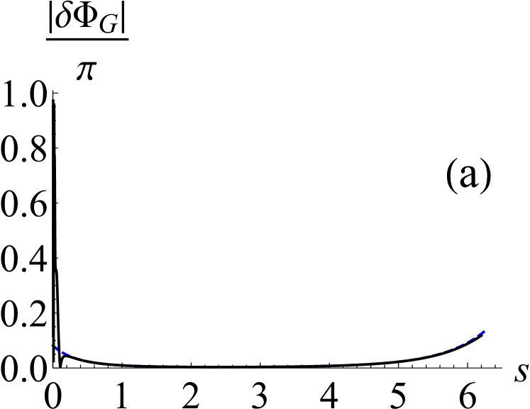
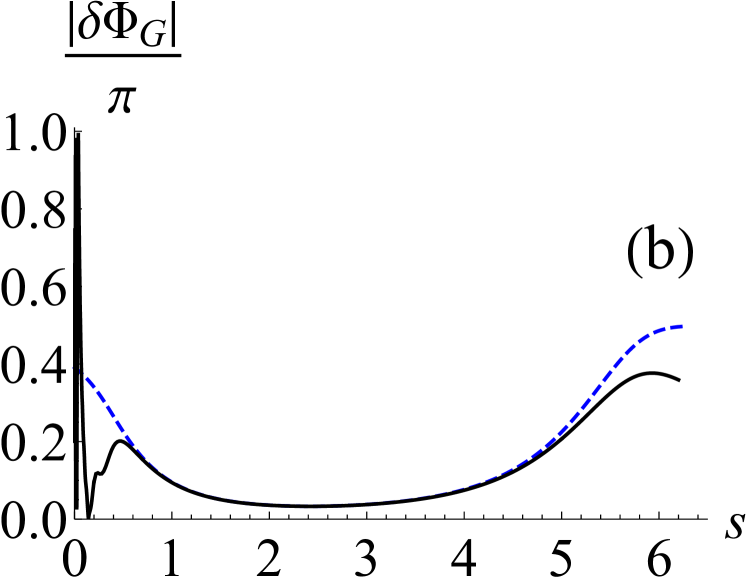
Figure 1: (Color online) Correction to the geometric phase $\delta\Phi_{G}\equiv\Phi_{G}-\Phi_{U}$ (where $\Phi_{U}=-\pi+\pi\cos\theta_{0}$) of the two-level system in the presence of the harmonic oscillator environment as a function of the Ohmicity parameter $s$ for weak system-environment coupling strength. The solid, black curve shows the geometric phase when the initial state is prepared via a projective measurement, while the dashed, blue curve is for an uncorrelated initial state [that is, the dynamics are given by Eq. (21)]. In (a), the system-environment coupling strength is $\lambda=0.01$, while in (b) we have used $\lambda=0.1$. Throughout, we are working in dimensionless units with $\hbar=1$, and here we have set $\omega_{0}=1$. We have used $\omega_{c}=5$, $\theta_{0}=\pi/3$, and $\beta\rightarrow\infty$ (zero temperature).

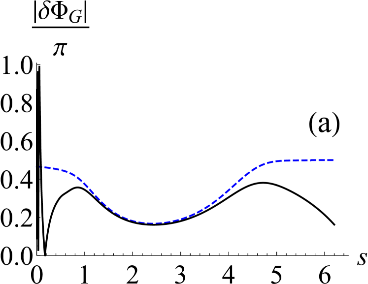
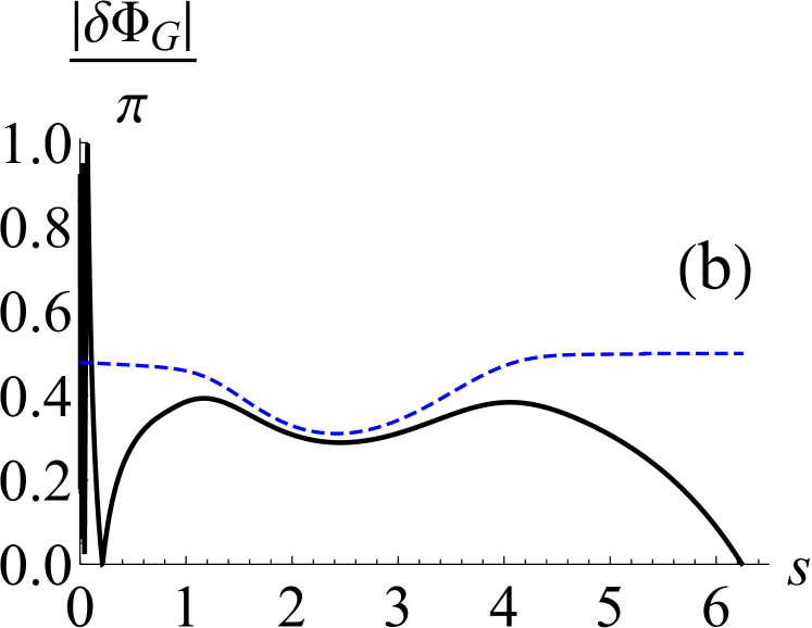
Figure 2: (Color online) Same as Fig 1 except that in (a), we have $\lambda=0.5$ and in (b), we have $\lambda=1$.

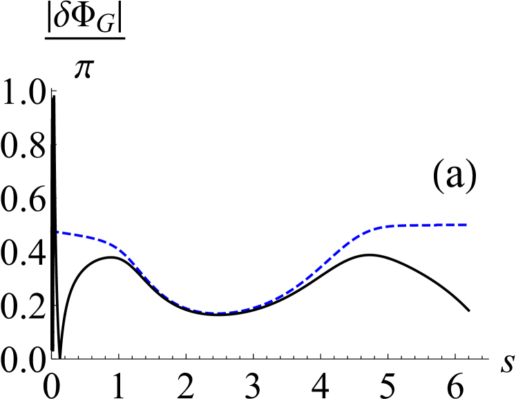
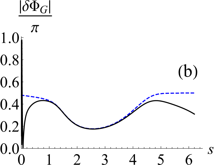
Figure 3: (Color online) Same as Fig. 1, except that the system-environment coupling strength is $\lambda=0.5$, and in (a), we have $\beta=2$, while in (b) we have $\beta=1$.

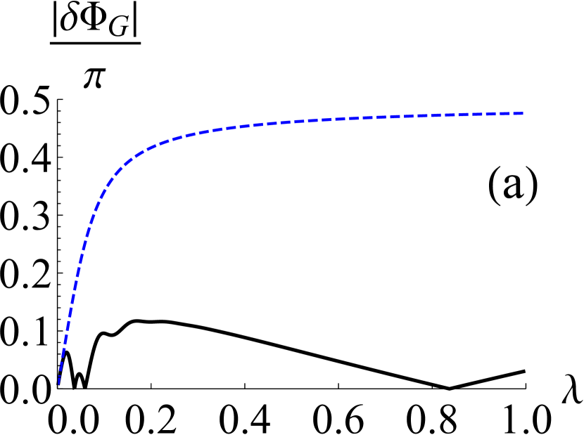
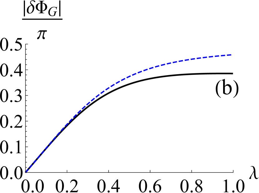
Figure 4: Color online) Correction to the geometric phase $\delta\Phi_{G}\equiv\Phi_{G}-\Phi_{U}$ (where $\Phi_{U}=-\pi+\pi\cos\theta_{0}$) with a harmonic oscillator environment as a function of the system-environment coupling strength $\lambda$. The solid, black curve shows the geometric phase when the initial state is prepared via a projective measurement, while the dashed, blue curve is for an uncorrelated initial state. In (a), the Ohmicity parameters is $s=0.2$, while for (b), $s=1$. These results are obtained for $\beta\rightarrow\infty$ (zero temperature). As before, we have set $\omega_{0}=1$, and we have used $\omega_{c}=5$ and $\theta_{0}=\pi/3$.

If the initial system state $\left|\psi\right\rangle$ is prepared by a projective measurement, described by the projector $P_{\psi}=\left|\psi\right\rangle\left\langle\psi\right|$, then the initial system-environment state is $\rho(0)=\frac{1}{Z}P_{\psi}e^{-\beta H}P_{\psi}$ with $Z=\text{Tr}_{S,B}[P_{\psi}e^{-\beta H}]$. With this initial state, the evolution of the off-diagonal elements of the system density matrix is given by Morozov et al. (2012); Chaudhry and Gong (2013a)

$$\langle\sigma_{\pm}(t)\rangle=\langle\sigma_{\pm}\rangle e^{\pm i[\omega_{0}t+\chi(t)]}e^{-\Gamma(t)},$$ (22)

where

$$\Gamma(t)=\Gamma_{\text{uc}}(t)+\Gamma_{\text{corr}}(t),$$

$$\Gamma_{\text{corr}}(t)=$$

$$-\frac{1}{2}\ln\bigg{[}1-\frac{(1-\cos^{2}\theta_{0})\sin^{2}[\Phi(t)]}{[\cosh(\beta\omega_{0}/2)-\cos\theta_{0}\sinh(\beta\omega_{0}/2)]^{2}}\bigg{]},$$

$$\tan[\chi(t)] =\frac{\sinh(\beta\omega_{0}/2)-\cos\theta_{0}\cosh(\beta\omega_{0}/2)}{\cosh(\beta\omega_{0}/2)-\cos\theta_{0}\sinh(\beta\omega_{0}/2)}\tan[\Phi(t)],$$

$$\Phi(t) =\sum_{k}\frac{4|g_{k}|^{2}}{\omega_{k}^{2}}\sin(\omega_{k}t).$$

For completeness, the derivation of these results is sketched in Appendix A. Note that the effect of the initial correlations is to modify the decoherence rate as well as to introduce a phase shift. Moreover, for zero temperature, these expressions further simplify to $\Gamma_{\text{corr}}(t)=0$ and $\chi(t)=\Phi(t)$. In this case, the decoherence rate is not modified and the effect of the initial correlations is a simple phase shift given by $\Phi(t)$.

With the system density matrix found, the geometric phase can then be evaluated. To calculate the sum over the environment modes, the sum is converted to an integral via the spectral density $J(\omega)$, which allows us to write $\sum_{k}4|g_{k}|^{2}(\ldots)$ as $\int_{0}^{\infty}\,d\omega\,J(\omega)(\ldots)$. We consider the spectral density to be of the form $J(\omega)=\lambda\omega^{s}\omega_{c}^{1-s}e^{-\omega/\omega_{c}}$, where $\lambda$ is a dimensionless constant characterizing the system-environment interaction strength, $s$ is the so-called Ohmicity parameter, and $\omega_{c}$ is the cutoff frequency Breuer and Petruccione (2007). In Figs. 1(a) and (b), we have plotted the behavior of the correction to the geometric phase $|\delta\Phi_{G}|$, as the Ohmicity parameter is varied, for weak system-environment coupling strength. It is clear from these figures that for weak system-environment coupling strength, the effect of the initial correlations on the geometric phase is generally negligible since the dashed blue line largely overlaps with the solid black curve. Nevertheless, for sub-Ohmic environments (that is, $s<1$), the initial correlations can still play a role. Interestingly, taking the initial correlations into account generally makes the correction to the geometric phase smaller. In fact, for a particular value of the Ohmicity parameter, the correction to the geometric phase is zero. Proceeding along these lines, in Figs. 2(a) and (b) we have shown the correction to the geometric phase at zero temperature for stronger system-environment coupling strengths. Three points are evident from these figures. First, for a range of values of $s$, the initial correlations have a very small effect on the geometric phase. Second, for sub-Ohmic environments as well as for very super-Ohmic environments, the contribution of the initial correlations to the geometric phase is very significant. Third, the initial correlations generally reduce the correction to the geometric phase, thereby implying that the initial correlations increase the robustness of the geometric phase. As before, for a particular value of the Ohmicity parameter, the correction to the geometric phase becomes zero. We have also found that, as expected, as the temperature is increased, the effect of the initial correlations decreases [see Figs. 3(a) and (b)].

It is also interesting to analyze the correction to the geometric phase as the system-environment couping strength is varied. The results are illustrated in Fig. 4(a) and (b). For the sub-Ohmic environment considered in Fig. 4(a), the initial correlations greatly reduce the correction to the geometric phase. Surprisingly, as the system-environment coupling strength is increased, the correction to the geometric phase, in the case where the initial correlations are taken into account, can decrease. In fact, for particular non-zero values of the system-environment interaction strength, the correction to the geometric phase becomes zero. This is not the case for an Ohmic environment [see Fig. 4(b)].

III.2 System state preparation by unitary operation

We now analyze the effect of the initial correlations if a unitary operation, instead of a projective measurement, is used to prepare the initial system state. The initial system-environment state in this case is $\rho(0)=\frac{1}{Z}\Omega e^{-\beta H}\Omega^{\dagger}$, where $\Omega$ is a unitary operation performed on the system. The off-diagonal elements of the system density matrix are given by Morozov et al. (2012); Chaudhry and Gong (2013a)

$$\langle\sigma_{\pm}(t)\rangle=\langle\sigma_{\pm}(0)\rangle e^{\pm i[\omega_{0}t+\chi(t)]}e^{-\Gamma(t)},$$ (23)

with

$$\Gamma(t) =\Gamma_{\text{uc}}(t)+\Gamma_{\text{corr}}(t),$$ (24)

where

$$\Gamma_{\text{corr}}(t) =-\ln\left\{\text{abs}\left[\frac{e^{-\beta\omega_{0}/2}\langle 0|\Omega^{\dagger}\sigma_{+}\Omega|0\rangle e^{-i\Phi(t)}+e^{\beta\omega_{0}/2}\langle 1|\Omega^{\dagger}\sigma_{+}\Omega|1\rangle e^{+i\Phi(t)}}{e^{-\beta\omega_{0}/2}\langle 0|\Omega^{\dagger}\sigma_{+}\Omega|0\rangle+e^{\beta\omega_{0}/2}\langle 1|\Omega^{\dagger}\sigma_{+}\Omega|1\rangle}\right]\right\},$$ (25)

$$\chi(t) =\arg\bigg{[}\cos[\Phi(t)]+i\sin[\Phi(t)]\bigg{(}\frac{\langle 1|\Omega^{\dagger}\sigma_{+}\Omega|1\rangle e^{\beta\omega_{0}/2}-\langle 0|\Omega^{\dagger}\sigma_{+}\Omega|0\rangle e^{-\beta\omega_{0}/2}}{\langle 1|\Omega^{\dagger}\sigma_{+}\Omega|1\rangle e^{\beta\omega_{0}/2}+\langle 0|\Omega^{\dagger}\sigma_{+}\Omega|0\rangle e^{-\beta\omega_{0}/2}}\bigg{)}\bigg{]}.$$ (26)

Here $\left|0\right\rangle$ and $\left|1\right\rangle$ are the eigenstates of $\sigma_{z}$ with $\sigma_{z}\left|l\right\rangle=(-1)^{l}\left|l\right\rangle$. These derivations are again sketched in Appendix A. One can check from these expressions that for zero temperature, $\Gamma_{\text{corr}}=0$ and $\chi(t)=\Phi(t)$. Consequently, the behavior of the geometric phase at zero temperature is the same as when the initial system state is prepared via a projective measurement. However, there will be differences at non-zero temperatures. The correction to the geometric phase $\delta\Phi_{G}=\Phi_{G}-\Phi_{0}$, where $\Phi_{0}$ is the geometric phase for the two-level system if the system-environment coupling strength is zero, is plotted as a function of the Ohmicity parameter $s$ for two different temperatures in Fig. 5 for moderate system-environment coupling strength. Once again, it is clear that the initial correlations can play a very significant role for the geometric phase, especially for sub-Ohmic environments.

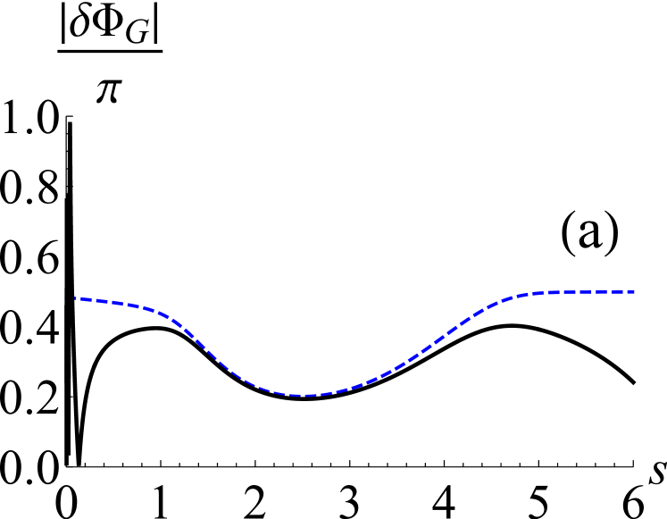
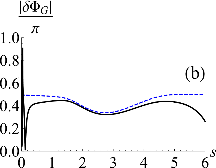
Figure 5: (Color online) Correction to the geometric phase $\delta\Phi_{G}\equiv\Phi_{G}-\Phi_{0}$ (where $\Phi_{0}$ is the geometric phase for the two-level system if the system-environment interaction strength is zero) with a harmonic oscillator environment as a function of the Ohmicity parameter $s$ if the initial state is prepared via a unitary operation. The solid, black curve shows the geometric phase when the initial state is prepared via the unitary operation $\Omega=e^{i\pi\sigma_{y}/3}$, while the dashed, blue curve is for an uncorrelated initial state. In (a), we have $\beta=3$ while in (b), we have $\beta=1$. Once again, we have set $\omega_{0}=1$, and we have used $\omega_{c}=5$ and $\lambda=0.5$.

IV Two-level system interacting with spin environment

We now consider the central two-level system to be interacting with a collection of $N$ two-level systems Cucchietti et al. (2005); Camalet and Chitra (2007); Schlosshauer (2007); Villar (2009). The system Hamiltonian $H_{S}$ is still $\frac{\omega_{0}}{2}\sigma_{z}$, while the environment Hamiltonian is now $\sum_{i}\omega_{i}\sigma^{i}_{x}$, and the system-environment interaction is described by $\sigma_{z}\sum_{i}\lambda_{i}\sigma_{z}^{i}$. Since $[H_{S},H_{SB}]=0$, this is also a pure dephasing model. If the initial system-environment state is a product state of the form $\rho(0)=\rho_{S}(0)\otimes e^{-\beta H_{B}}/Z_{B}$, then the evolution of the off-diagonal elements is given by Camalet and Chitra (2007); Villar (2009)

$$\langle\sigma_{\pm}(t)\rangle =\langle\sigma_{\pm}\rangle e^{\pm i\omega_{0}t}e^{-\Gamma_{\text{uc}}(t)},$$

where

$$\Gamma_{\text{uc}}(t)=-\sum_{j}\ln\bigg{\{}1-\frac{2\lambda_{j}^{2}}{\lambda_{j}^{2}+\omega_{j}^{2}}\sin^{2}(\sqrt{\lambda_{j}^{2}+\omega_{j}^{2}}t)\bigg{\}},$$

and the sum is over the environment spins. The derivation of this result is reproduced in Appendix B. However, as emphasized before, this result may questionable since the initial system-environment correlations are disregarded. To investigate the effect of these correlations, we consider the system state to be prepared by a projective measurement as well as by a unitary operation starting from the total system-environment equilibrium state $e^{-\beta H}/Z$. We note that, to the best of our knowledge, this model has not been solved taking initial correlations into account before.

IV.1 System state preparation by projective measurement

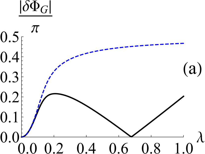
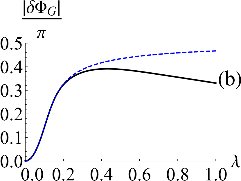
Figure 6: (Color online) Behavior of the correction to the geometric phase $\delta\Phi_{G}=\Phi_{G}-\Phi_{U}$ [here $\Phi_{U}=\pi(\cos\theta_{0}-1)$] as the spin-spin environment coupling strength $\lambda$ is varied, both with (solid, black) and without (dashed, blue) initial correlations when the initial state is prepared via a projective measurement. We have considered the environment to be a spin bath with $N=50$, and for simplicity, we have assumed that the interaction strength between the central spin and each environment spin is the same (that is, $\lambda_{j}=\lambda$ for all $j$). As always, we are working in dimensionless units with $\hbar=1$ and here have set $\omega_{i}=1$ for all $i$. In (a), we have used zero temperature $(\beta\rightarrow\infty)$, while in (b), $\beta=0.4$. Also, $\omega_{0}=5$ and $\theta_{0}=\pi/3$.

If the initial state is $\rho(0)=P_{\psi}e^{-\beta H}P_{\psi}/Z$, then the off-diagonal elements of the density matrix are given by

$$\langle\sigma_{\pm}(t)\rangle =\langle\sigma_{\pm}\rangle e^{\pm i[\omega_{0}t+\chi(t)]}e^{-\Gamma(t)},$$ (27)

where, similar to the form obtained for the harmonic oscillator environment,

$$\tan[\chi(t)] =\frac{\sinh(\beta\omega_{0}/2)-\cos\theta_{0}\cosh(\beta\omega_{0}/2)}{\cosh(\beta\omega_{0}/2)-\cos\theta_{0}\sinh(\beta\omega_{0}/2)}\tan[\Phi(t)],$$

with $\theta_{0}$ the Bloch angle characterizing the initial state. We now have

$$\Phi(t)=\sum_{j}\arg\big{[}A_{j}(t)+iB_{j}(t)\big{]},$$ (28)

where $A_{j}(t)=1-2\frac{\lambda_{j}^{2}}{\alpha_{j^{2}}}\sin^{2}(\alpha_{j}t)$ and $B_{j}(t)=\frac{\lambda_{j}^{2}}{\alpha_{j}^{2}}\tanh(\beta\alpha_{j})\sin(2\alpha_{j}t)$ with $\alpha_{j}=\sqrt{\lambda_{j}^{2}+\omega_{j}^{2}}$. Also, $\Gamma(t)=\Gamma_{\text{uc}}(t)+\Gamma_{\text{corr}}(t)$, where $\Gamma_{\text{corr}}(t)=\Gamma_{\text{corr}}^{(1)}(t)+\Gamma_{\text{corr}}^{(2)}(t)$, and

$$\Gamma_{\text{corr}}^{(1)}(t) =-\frac{1}{2}\sum_{j}\ln\bigg{[}1+(\lambda_{j}/\omega_{j})^{4}\bigg{(}\frac{\tanh(\beta\alpha_{j})\sin(2\alpha_{j}t)}{1+(\lambda_{j}/\omega_{j})^{2}\cos(2\alpha_{j}t)}\bigg{)}^{2}\bigg{]},$$ (29)

$$\Gamma_{\text{corr}}^{(2)}(t) =-\frac{1}{2}\ln\bigg{[}1-\frac{(1-\cos^{2}\theta_{0})\sin^{2}[\Phi(t)]}{[\cosh(\beta\omega_{0}/2)-\cos\theta_{0}\sinh(\beta\omega_{0}/2)]^{2}}\bigg{]}.$$ (30)

Interestingly, in this case, even if the temperature is zero, the initial correlations change the decay rate of the off-diagonal elements since $\Gamma_{\text{corr}}^{(1)}(t)\neq 0$ at zero temperature while $\Gamma_{\text{corr}}^{(2)}(t)=0$. On the other hand, at zero temperature, $\chi(t)$ is once again equal to $\Phi(t)$.

With the system density matrix found, we compute the correction to the geometric phase $\delta\Phi_{G}=\Phi_{G}-\Phi_{U}$. The behavior of the correction $\delta\Phi_{G}$ as a function of the two-level system-environment coupling strength is shown in Figs. 6(a) and (b). The effect of the initial correlations is again very significant; in particular, the initial correlations can make the geometric phase more robust. For particular values of the system-environment interaction strength $\lambda$, the correction to the geometric phase becomes zero.

IV.2 System state preparation by unitary operation

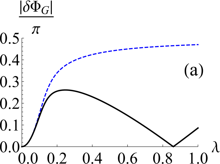
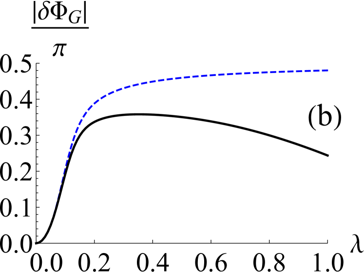
Figure 7: (Color online) Behavior of the correction to geometric phase $\delta\Phi_{G}=\Phi_{G}-\Phi_{0}$ (here $\Phi_{0}$ is the geometric phase when the system-environment coupling strength is zero) as the spin-spin environment coupling strength $\lambda$ is varied, both with (solid, black) and without (dashed, blue) initial correlations when the initial state is prepared by a unitary operation. As before, we have considered the environment to be a spin bath with $N=50$, and $\lambda_{j}=\lambda$ for all $j$. Once again, we are working in dimensionless units with $\hbar=1$ and here have set $\omega_{i}=1$ for all $i$. In (a), we have used $\beta=1$, while in (b), $\beta=0.4$. Also, $\omega_{0}=5$ and $\Omega=e^{i\pi\sigma_{y}/3}$.

We now prepare the initial system state via a unitary operation. We find that for the initial system-environment state $\rho(0)=\frac{1}{Z}\Omega e^{-\beta H}\Omega^{\dagger}$, the off-diagonal elements of the density matrix are, as for the harmonic oscillator environment,

$$\langle\sigma_{\pm}(t)\rangle=\langle\sigma_{\pm}(0)\rangle e^{\pm i[\omega_{0}t+\chi(t)]}e^{-\Gamma(t)},$$ (31)

where $\Gamma(t)=\Gamma_{\text{uc}}(t)+\Gamma_{\text{corr}}^{(1)}(t)+\Gamma_{\text{corr}}^{(2)}(t)$ with $\Gamma_{\text{corr}}^{(1)}(t)$ the same as before [see Eq. (29)], while $\Gamma_{\text{corr}}^{(2)}(t)$ is given by

$$\Gamma_{\text{corr}}^{(2)}(t) =-\ln\left\{\text{abs}\left[\frac{e^{-\beta\omega_{0}/2}\langle 0|\Omega^{\dagger}\sigma_{+}\Omega|0\rangle e^{-i\Phi(t)}+e^{\beta\omega_{0}/2}\langle 1|\Omega^{\dagger}\sigma_{+}\Omega|1\rangle e^{i\Phi(t)}}{e^{-\beta\omega_{0}/2}\langle 0|\Omega^{\dagger}\sigma_{+}\Omega|0\rangle+e^{\beta\omega_{0}/2}\langle 1|\Omega^{\dagger}\sigma_{+}\Omega|1\rangle}\right]\right\}.$$

Also, $\chi(t)$ is of the same form as in Eq. (26), but with $\Phi(t)$ now given by Eq. (28). Details can be found in Appendix B. Once again, for zero temperature, we find that the dynamics are the same as the case where the initial state is prepared by a projective measurement. However, as illustrated in Figs. 7(a) and (b), even for non-zero temperatures, the contribution to the geometric phase due to the initial correlations can be very significant. Once again, if we increase the temperature, the effect of the initial correlations decreases as expected.

V Conclusion

In summary, we have presented exact expressions for the geometric phase of a two-level system undergoing pure dephasing to investigate the effect of the initial system-environment correlations on the geometric phase. As concrete examples, we have applied these expressions to two different environments: a collection of harmonic oscillators, and a collection of spins. Our results illustrate that the effect of the initial correlations on the geometric phase can be very significant, with a non-trivial dependence on the system-environment parameters. For instance, increasing the system-environment coupling strength may not always increase the correction to the geometric phase; in fact, for certain values of the coupling strength, the correction becomes zero, implying that the initial correlations can increase the robustness of the geometric phase. Our work on the geometric phase should be important not only for studies of the geometric phase itself as well as its practical implementations, but also for investigating the role of system-environment correlations in open quantum systems.

Appendix A Solution for harmonic oscillator environment

For completeness, we sketch how to solve for the system dynamics for the total system-environment Hamiltonian $H=H_{S}+H_{B}+H_{SB}$, where Morozov et al. (2012); Chaudhry and Gong (2013a)

$$H_{S}=\frac{\omega_{0}}{2}\sigma_{z},\;H_{B}=\sum_{k}\omega_{k}b_{k}^{\dagger}b_{k},$$

$$H_{SB}=\sigma_{z}\sum_{k}(g_{k}^{*}b_{k}+g_{k}b_{k}^{\dagger}).$$

First, we transform to the interaction picture to obtain

$$H_{I}(t) =e^{i(H_{S}+H_{B})t}H_{\text{SB}}e^{-i(H_{S}+H_{B})t},$$

$$=\sigma_{z}\sum_{k}(g_{k}^{*}b_{k}e^{-i\omega_{k}t}+g_{k}b_{k}^{\dagger}e^{i\omega_{k}t}).$$ (32)

We next find the time evolution operator $U_{I}(t)$ corresponding to $H_{I}(t)$ using the Magnus expansion as

$$U_{I}(t)=\exp\{\sigma_{z}\sum_{k}[b_{k}^{\dagger}\alpha_{k}(t)-b_{k}\alpha_{k}^{*}(t)]/2\},$$ (33)

and the total unitary time-evolution operator is $U(t)=e^{-i\omega_{0}\sigma_{z}t/2}U_{I}(t)$. We now define $[\rho_{S}(t)]_{10}=\text{Tr}_{S,B}[U(t)\rho(0)U^{\dagger}(t)\left|0\right\rangle\left\langle 1\right|]$. Defining $P_{01}(t)=U^{\dagger}(t)\left|0\right\rangle\left\langle 1\right|U(t)$, this can be written as $[\rho_{S}(t)]_{10}=\text{Tr}_{S,B}[\rho(0)P_{01}(t)]$. Simplifying $P_{01}(t)$ using the unitary time-evolution operator $U(t)$, we find that

$$P_{01}(t)=e^{i\omega_{0}t}e^{-R_{01}(t)}P_{01},$$ (34)

where

$$R_{01}(t)=\sum_{k}[b_{k}^{\dagger}\alpha_{k}(t)-b_{k}\alpha_{k}^{*}(t)],$$ (35)

with

$$\alpha_{k}(t)=\frac{2g_{k}(1-e^{i\omega_{k}t})}{\omega_{k}}.$$

Consequently,

$$[\rho_{S}(t)]_{10}=e^{i\omega_{0}t}\text{Tr}_{S,B}[e^{-R_{01}(t)}P_{01}\rho(0)].$$ (36)

This is a general result because it applies to an arbitrary initial density $\rho(0)$. Now, if $\rho(0)=\rho_{S}(0)\otimes\rho_{B}$, where $\rho_{B}=\frac{e^{-\beta H_{B}}}{Z_{B}}$ with $Z_{B}=\text{Tr}_{B}[e^{-\beta H_{B}}]$, then

$$[\rho_{S}(t)]_{10}=[\rho_{S}(0)]_{10}e^{i\omega_{0}t}\text{Tr}_{B}[e^{-R_{01}(t)}\rho_{B}].$$ (37)

The trace over the environment computes to

$$\text{Tr}_{B}[e^{-R_{01}(t)}\rho_{B}]=$$

$$\exp\left[-\sum_{k}4|g_{k}|^{2}\frac{[1-\cos(\omega_{k}t)]}{\omega_{k}^{2}}\coth\left(\frac{\beta\omega_{k}}{2}\right)\right],$$ (38)

thereby yielding

$$[\rho_{S}(t)]_{10}=[\rho_{S}(0)]_{10}e^{i\omega_{0}t}e^{-\Gamma_{\text{uc}}(t)},$$ (39)

with

$$\Gamma_{\text{uc}}(t)=\sum_{k}4|g_{k}|^{2}\frac{[1-\cos(\omega_{k}t)]}{\omega_{k}^{2}}\coth\left(\frac{\beta\omega_{k}}{2}\right).$$ (40)

We now consider what happens if the initial state is of the form $\rho(0)=\frac{1}{Z}\Omega e^{-\beta H}\Omega^{\dagger}$, with $Z$ the normalization factor. Currently, the $\Omega$ operator can be a projection operator or a unitary operator. To first simplify $Z$, we use the completeness relation $\sum_{l}\left|l\right\rangle\left\langle l\right|=\mathds{1}$, where $\sigma_{z}\left|l\right\rangle=(-1)^{l}\left|l\right\rangle$. Then,

$$Z =\sum_{l}e^{-\beta\omega_{0}(-1)^{l}/2}\langle l|\Omega^{\dagger}\Omega|l\rangle\text{Tr}_{B}[e^{-\beta H_{B}^{(l)}}],$$ (41)

with

$$H_{B}^{(l)}=H_{B}+(-1)^{l}\sum_{k}(g_{k}^{*}b_{k}+g_{k}b_{k}^{\dagger}).$$ (42)

To simplify further, we introduce the displaced harmonic oscillator modes

$$B_{k,l}=b_{k}+\frac{(-1)^{l}g_{k}}{\omega_{k}},$$ (43)

$$B_{k,l}^{\dagger}=b_{k}^{\dagger}+\frac{(-1)^{l}g_{k}^{*}}{\omega_{k}},$$ (44)

allowing us to write

$$Z=\sum_{l}e^{-\beta\omega_{0}(-l)^{l}/2}\langle l|\Omega^{\dagger}\Omega|l\rangle e^{\beta\sum_{k}\frac{|g_{k}|^{2}}{\omega_{k}}}Z_{B},$$ (45)

where $Z_{B}=\text{Tr}_{B}[e^{-\beta\sum_{k}\omega_{k}B_{k,l}^{\dagger}B_{k,l}}]$. With $Z$ found, we then substitute our initial state in Eq. (36) and introduce $\sum_{l}\left|l\right\rangle\left\langle l\right|$ to simplify the resulting $\text{Tr}_{B}[e^{-R_{01}(t)}e^{-\beta H_{B}^{(l)}}]$. Using the displaced harmonic oscillator modes as before, we find that

$$R_{01}(t)=\sum_{k}[\alpha_{k}(t)B_{k,l}^{\dagger}-\alpha_{k}^{*}(t)B_{k,l}]+i(-1)^{l}\Phi(t),$$ (46)

where

$$\Phi(t) = \sum_{k}\frac{4|g_{k}|^{2}}{\omega_{k}^{2}}\sin(\omega_{k}t).$$ (47)

We then find that

$$\text{Tr}_{B}[e^{-R_{01}(t)}e^{-\beta H_{B}^{(l)}}]=e^{-i(-1)^{l}\Phi(t)}Z_{B}e^{\beta\sum_{k}\frac{|g_{k}|^{2}}{\omega_{k}}}e^{-\Gamma_{\text{uc}}(t)}.$$ (48)

Putting this all together, and rearranging, we obtain

$$[\rho_{S}(t)]_{10} =[\rho_{S}(0)]_{10}e^{i\omega_{0}t}e^{-\Gamma_{\text{uc}}(t)}X(t),$$ (49)

with

$$X(t)=\dfrac{\sum_{l}\langle l|\Omega^{\dagger}P_{01}\Omega|l\rangle e^{-i(-1)^{l}\Phi(t)}e^{-\beta\omega_{0}(-1)^{l}/2}}{\sum_{l}\langle l|\Omega^{\dagger}P_{01}\Omega|l\rangle e^{-\beta\omega_{0}(-1)^{l}/2}}.$$

Now assuming that $\Omega$ is a projection operator, that is, $\Omega=\left|\psi\right\rangle\left\langle\psi\right|$, we can further simplify and write $X(t)$ in polar form to obtain Eq. (22). On the other hand, if $\Omega$ is taken to be a unitary operator, we obtain Eq. (23).

Appendix B Dynamics with a spin environment

We now consider the total system-environment Hamiltonian $H=H_{S}+H_{B}+H_{SB}$, where

$$H_{S}=\frac{\omega_{0}}{2}\sigma_{z},\;H_{B}=\sum_{i}\omega_{i}\sigma^{i}_{x},\>\>H_{SB}=\sigma_{z}\otimes\sum_{i}\lambda_{i}\sigma_{z}^{i}.$$

Once again, since $[H_{S},H_{SB}]=0$, this is a pure dephasing model. Our aim is to then calculate $\langle\sigma_{\pm}(t)\rangle$. We note that $e^{it(H_{B}+H_{SB})}\left|l\right\rangle=e^{it(H_{B}+(-1)^{l}V)}\left|l\right\rangle$, where

$$V=\sum_{i}\lambda_{i}\sigma_{z}^{i}.$$ (50)

Using the completeness relation $\sum_{s}\left|l\right\rangle\left\langle l\right|=\mathds{1}$, we can simplify $\sigma_{\pm}(t)=e^{iHt}\sigma_{\pm}e^{-iHt}$ to find

$$\sigma_{\pm}(t) =e^{\pm i\omega_{0}t}e^{it(H_{B}\pm V)}e^{-it(H_{B}\mp V)}\sigma_{\pm}.$$ (51)

We now consider initial states of the form

$$\rho(0) =\rho_{S}(0)\otimes\rho_{B},\>\>\>\rho_{B}=e^{-\beta H_{B}}/Z_{B}.$$ (52)

For simplicity, we only show the calculation for $\langle\sigma_{+}(t)\rangle$. Using Eq. (51), we obtain

$$\langle\sigma_{+}(t)\rangle=\text{Tr}[\sigma_{+}(t)\rho(0)]$$

$$=\frac{e^{i\omega_{0}t}}{Z_{B}}\langle\sigma_{+}(0)\rangle\text{Tr}_{B}[R(t)e^{-\beta H_{B}}],$$ (53)

where $R(t)=e^{it(H_{B}+V)}e^{-it(H_{B}-V)}$. Our remaining task is to compute $\text{Tr}_{B}[R(t)e^{-\beta H_{B}}]$. To this end, we first write $R(t)$ as $e^{it\sum_{j}\alpha_{j}(\vec{n}_{1}^{j}\cdot\vec{\sigma}_{j})}e^{-it\sum_{j}\alpha_{j}(\vec{n}_{2}^{j}\cdot\vec{\sigma}_{j})}$, where $\vec{n}_{1}^{j}=\frac{1}{\alpha_{j}}(\omega_{j},0,\lambda_{j})$, $\vec{n}_{2}^{j}=\frac{1}{\alpha_{j}}(\omega_{j},0,-\lambda_{j})$ and $\alpha_{j}=\sqrt{\omega_{j}^{2}+\lambda_{j}^{2}}$. The exponentials can then be combined and the resulting expression is further simplified to obtain

$$\text{Tr}_{B}[R(t)e^{-\beta H_{B}}]=2^{N}\prod_{j}\cos c_{j}\cos(i\beta\omega_{j}),$$ (54)

where $\cos c_{j}=1-2\bigg{(}\frac{\lambda_{j}}{\alpha_{j}}\bigg{)}^{2}\sin^{2}(\alpha_{j}t)$, and $Z_{B}=2^{N}\Pi_{j}\cos(i\beta\omega_{j})$. Putting it all together, we finally have that

$$\langle\sigma_{+}(t)\rangle=\langle\sigma_{+}(0)\rangle e^{i\omega_{0}t}\prod_{j}\bigg{\{}1-2\bigg{(}\frac{\lambda_{j}}{\alpha_{j}}\bigg{)}^{2}\sin^{2}(\alpha_{j}t)\bigg{\}}.$$ (55)

We now consider initially correlated states of the form

$$\rho(0) =\frac{1}{Z}\Omega e^{-\beta H}\Omega^{\dagger}$$

As before, we find that $\langle\sigma_{+}(t)\rangle=\text{Tr}_{S,B}[e^{i\omega_{0}t}R(t)\sigma_{+}\rho(0)]$. To simplify $\rho(0)$, we use the fact that $e^{-\beta H}\left|s\right\rangle=e^{(-1)^{s+1}\beta\omega_{0}/2}e^{-\beta(H_{B}+(-1)^{s}V)}\left|s\right\rangle$. We then have

$$\langle\sigma_{+}(t)\rangle =\frac{e^{i\omega_{0}t}}{Z}\bigg{[}\langle 0|\Omega^{\dagger}\sigma_{+}\Omega|0\rangle e^{-\beta\omega_{0}/2}\text{Tr}_{B}[R(t)e^{-\beta(H_{B}+V)}]$$

$$+\langle 1|\Omega^{\dagger}\sigma_{+}\Omega|1\rangle e^{\beta\omega_{0}/2}\text{Tr}_{B}[R(t)e^{-\beta(H_{B}-V)}]\bigg{]}.$$ (56)

We now sketch the calculation for $\text{Tr}_{B}[R(t)e^{-\beta(H_{B}+V)}]$ as the calculation for $\text{Tr}_{B}[R(t)e^{-\beta(H_{B}-V)}]$ is very similar. The trick is to write $\text{Tr}_{B}[R(t)e^{-\beta(H_{B}+V)}]$ as $\text{Tr}_{B}[e^{-it(H_{B}-V)}e^{i\gamma(H_{B}+V)}]$ we have defined $\gamma=t+i\beta$. The exponentials can then be manipulated as before to obtain

$$\text{Tr}_{B}[R(t)e^{-\beta(H_{B}+V)}]=C_{0}\Pi_{j}\left(A_{j}-iB_{j}\right),$$

where $A_{j}=1-2(\frac{\lambda_{j}}{\alpha_{j}})^{2}\sin^{2}(\alpha_{j}t)$, $B_{j}=2(\frac{\lambda_{j}}{\alpha_{j}})^{2}\tanh(\beta\alpha_{j})\sin(\alpha_{j}t)\cos(\alpha_{j}t)$, and $C_{0}=\Pi_{j}2\cosh(\beta\alpha_{j})$. We can then further simplify to

$$\langle\sigma_{+}(t)\rangle= \langle\sigma_{+}\rangle e^{i\omega_{0}t}e^{-\Gamma(t)}\times$$

$$\frac{\sum_{l}\langle l|\Omega^{\dagger}\sigma_{+}\Omega|l\rangle e^{-\beta\omega_{0}(-1)^{l}/2}e^{-i(-1)^{l}\Phi(t)}}{\sum_{l}\langle l|\Omega^{\dagger}\sigma_{+}\Omega|l\rangle e^{-\beta\omega_{0}(-1)^{l}/2}},$$

where

$$\Gamma(t) =\sum_{j}\Gamma_{j}(t),\>\>\>\Phi(t)=\sum_{j}\Phi_{j}(t),$$ (57)

and $F_{j}(t)=A_{j}(t)+iB_{j}(t)=e^{-\Gamma_{j}(t)}e^{i\Phi_{j}(t)}$. It is then a simple matter of specifying that $\Omega$ is a projection operator or a unitary operator to work out the dynamics.

References

• Sjoqvist (2015) E. Sjoqvist, Geometric phases in quantum information, Int. J. Quantum Chem. 115, 1311 (2015).
• Cohen et al. (2019) E. Cohen, H. Larocque, F. Bouchard, F. Nejadsattari, Y. Gefen, and E. Karimi, Geometric phase from aharonov–bohm to pancharatnam–berry and beyond, Nat. Rev. Phys. 1, 437 (2019).
• Pancharatnam (1956) S. Pancharatnam, Generalized theory of interference and its applications, Proc. Indian Acad. Sci. A 44, 398 (1956).
• Longuet-Higgins (1975) H. Longuet-Higgins, The intersection of potential energy surfaces in polyatomic molecules, Proc. R. Soc. London A 344, 147 (1975).
• Stone (1976) A. J. Stone, Spin-orbit coupling and the intersection of potential energy surfaces in polyatomic molecules, Proc. R. Soc. London A 351, 141 (1976).
• Berry (1984) M. V. Berry, Quantal phase factors accompanying adiabatic changes, Proc. R. Soc. London A 392, 45 (1984).
• Aharonov and Anandan (1987) Y. Aharonov and J. Anandan, Phase change during a cyclic quantum evolution, Phys. Rev. Lett. 58, 1593 (1987).
• Uhlmann (1989) A. Uhlmann, On berry phases along mixtures of states, Ann. Phys. 501, 63 (1989).
• Sjöqvist et al. (2000) E. Sjöqvist, A. K. Pati, A. Ekert, J. S. Anandan, M. Ericsson, D. K. L. Oi, and V. Vedral, Geometric phases for mixed states in interferometry, Phys. Rev. Lett. 85, 2845 (2000).
• Suter et al. (1987) D. Suter, G. Chingas, R. Harris, and A. Pines, Berry’s phase in magnetic resonance, Mol. Phys. 61, 1327 (1987).
• Leek et al. (2007) P. J. Leek, J. M. Fink, A. Blais, R. Bianchetti, M. Göppl, J. M. Gambetta, D. I. Schuster, L. Frunzio, R. J. Schoelkopf, and A. Wallraff, Observation of berry’s phase in a solid-state qubit, Science 318, 1889 (2007).
• Simon et al. (1988) R. Simon, H. J. Kimble, and E. C. G. Sudarshan, Evolving geometric phase and its dynamical manifestation as a frequency shift: An optical experiment, Phys. Rev. Lett. 61, 19 (1988).
• Zanardi and Rasetti (1999) P. Zanardi and M. Rasetti, Holonomic quantum computation, Phys. Lett. A 264, 94 (1999).
• Jones et al. (2000) J. A. Jones, V. Vedral, A. Ekert, and G. Castagnoli, Geometric quantum computation using nuclear magnetic resonance, Nature 403, 869 (2000).
• Falci et al. (2000) G. Falci, R. Fazio, G. Massimo Palma, J. Siewert, and V. Vedral, Detection of geometric phases in superconducting nanocircuits, Nature 407, 355 (2000).
• Duan et al. (2001) L.-M. Duan, J. I. Cirac, and P. Zoller, Geometric manipulation of trapped ions for quantum computation, Science 292, 1695 (2001).
• Xiang-Bin and Keiji (2001) W. Xiang-Bin and M. Keiji, Nonadiabatic conditional geometric phase shift with nmr, Phys. Rev. Lett. 87, 097901 (2001).
• Liebfried et al. (2000) D. Liebfried, B. DeMarco, V. Meyer, D. Lucas, M. Barrett, J. Britton, W. M. Itano, B. Jelenkovic, C. Langer, T. Rosenband, and D. J. Wineland, Experimental demonstration of a robust, high-fidelity geometric two ion-qubit phase gate, Nature 422, 412 (2000).
• Ericsson et al. (2003) M. Ericsson, E. Sjöqvist, J. Brännlund, D. K. L. Oi, and A. K. Pati, Generalization of the geometric phase to completely positive maps, Phys. Rev. A 67, 020101 (2003).
• Carollo et al. (2003) A. Carollo, I. Fuentes-Guridi, M. F. m. c. Santos, and V. Vedral, Geometric phase in open systems, Phys. Rev. Lett. 90, 160402 (2003).
• Tong et al. (2004) D. M. Tong, E. Sjöqvist, L. C. Kwek, and C. H. Oh, Kinematic approach to the mixed state geometric phase in nonunitary evolution, Phys. Rev. Lett. 93, 080405 (2004).
• Whitney et al. (2005) R. S. Whitney, Y. Makhlin, A. Shnirman, and Y. Gefen, Geometric nature of the environment-induced berry phase and geometric dephasing, Phys. Rev. Lett. 94, 070407 (2005).
• Yi et al. (2006) X. X. Yi, D. M. Tong, L. C. Wang, L. C. Kwek, and C. H. Oh, Geometric phase in open systems: Beyond the markov approximation and weak-coupling limit, Phys. Rev. A 73, 052103 (2006).
• Lombardo and Villar (2006) F. C. Lombardo and P. I. Villar, Geometric phases in open systems: A model to study how they are corrected by decoherence, Phys. Rev. A 74, 042311 (2006).
• Dajka et al. (2008) J. Dajka, M. Mierzejewski, and J. Łuczka, Geometric phase of a qubit in dephasing environments, J. Phys. A: Math. Theor. 41, 012001 (2008).
• Lombardo and Villar (2010) F. C. Lombardo and P. I. Villar, Environmentally induced effects on a bipartite two-level system: Geometric phase and entanglement properties, Phys. Rev. A 81, 022115 (2010).
• Cucchietti et al. (2010) F. M. Cucchietti, J.-F. Zhang, F. C. Lombardo, P. I. Villar, and R. Laflamme, Geometric phase with nonunitary evolution in the presence of a quantum critical bath, Phys. Rev. Lett. 105, 240406 (2010).
• Villar and Lombardo (2011) P. I. Villar and F. C. Lombardo, Geometric phases in the presence of a composite environment, Phys. Rev. A 83, 052121 (2011).
• Lombardo and Villar (2013) F. C. Lombardo and P. I. Villar, Nonunitary geometric phases: A qubit coupled to an environment with random noise, Phys. Rev. A 87, 032338 (2013).
• Lombardo and Villar (2015) F. C. Lombardo and P. I. Villar, Correction to the geometric phase by structured environments: The onset of non-markovian effects, Phys. Rev. A 91, 042111 (2015).
• Hakim and Ambegaokar (1985) V. Hakim and V. Ambegaokar, Quantum theory of a free particle interacting with a linearly dissipative environment, Phys. Rev. A 32, 423 (1985).
• Haake and Reibold (1985) F. Haake and R. Reibold, Strong damping and low-temperature anomalies for the harmonic oscillator, Phys. Rev. A 32, 2462 (1985).
• Grabert et al. (1988) H. Grabert, P. Schramm, and G.-L. Ingold, Quantum brownian motion: The functional integral approach, Phys. Rep. 168, 115 (1988).
• Smith and Caldeira (1990) C. M. Smith and A. O. Caldeira, Application of the generalized feynman-vernon approach to a simple system: The damped harmonic oscillator, Phys. Rev. A 41, 3103 (1990).
• Karrlein and Grabert (1997) R. Karrlein and H. Grabert, Exact time evolution and master equations for the damped harmonic oscillator, Phys. Rev. E 55, 153 (1997).
• Dávila Romero and Pablo Paz (1997) L. Dávila Romero and J. Pablo Paz, Decoherence and initial correlations in quantum brownian motion, Phys. Rev. A 55, 4070 (1997).
• Lutz (2003) E. Lutz, Effect of initial correlations on short-time decoherence, Phys. Rev. A 67, 022109 (2003).
• Banerjee and Ghosh (2003) S. Banerjee and R. Ghosh, General quantum brownian motion with initially correlated and nonlinearly coupled environment, Phys. Rev. E 67, 056120 (2003).
• van Kampen (2004) N. G. van Kampen, A new approach to noise in quantum mechanics, J. Stat. Phys. 115, 1057 (2004).
• Ban (2009) M. Ban, Quantum master equation for dephasing of a two-level system with an initial correlation, Phys. Rev. A 80, 064103 (2009).
• Campisi et al. (2009) M. Campisi, P. Talkner, and P. Hänggi, Fluctuation theorem for arbitrary open quantum systems, Phys. Rev. Lett. 102, 210401 (2009).
• Uchiyama and Aihara (2010) C. Uchiyama and M. Aihara, Role of initial quantum correlation in transient linear response, Phys. Rev. A 82, 044104 (2010).
• Dijkstra and Tanimura (2010) A. G. Dijkstra and Y. Tanimura, Non-markovian entanglement dynamics in the presence of system-bath coherence, Phys. Rev. Lett. 104, 250401 (2010).
• Smirne et al. (2010) A. Smirne, H.-P. Breuer, J. Piilo, and B. Vacchini, Initial correlations in open-systems dynamics: The jaynes-cummings model, Phys. Rev. A 82, 062114 (2010).
• Dajka and Łuczka (2010) J. Dajka and J. Łuczka, Distance growth of quantum states due to initial system-environment correlations, Phys. Rev. A 82, 012341 (2010).
• Zhang et al. (2010) Y.-J. Zhang, X.-B. Zou, Y.-J. Xia, and G.-C. Guo, Different entanglement dynamical behaviors due to initial system-environment correlations, Phys. Rev. A 82, 022108 (2010).
• Tan and Zhang (2011) H.-T. Tan and W.-M. Zhang, Non-markovian dynamics of an open quantum system with initial system-reservoir correlations: A nanocavity coupled to a coupled-resonator optical waveguide, Phys. Rev. A 83, 032102 (2011).
• Lee et al. (2012) C. K. Lee, J. Cao, and J. Gong, Noncanonical statistics of a spin-boson model: Theory and exact monte carlo simulations, Phys. Rev. E 86, 021109 (2012).
• Morozov et al. (2012) V. G. Morozov, S. Mathey, and G. Röpke, Decoherence in an exactly solvable qubit model with initial qubit-environment correlations, Phys. Rev. A 85, 022101 (2012).
• Semin et al. (2012) V. Semin, I. Sinayskiy, and F. Petruccione, Initial correlation in a system of a spin coupled to a spin bath through an intermediate spin, Phys. Rev. A 86, 062114 (2012).
• Chaudhry and Gong (2013a) A. Z. Chaudhry and J. Gong, Amplification and suppression of system-bath-correlation effects in an open many-body system, Phys. Rev. A 87, 012129 (2013a).
• Chaudhry and Gong (2013b) A. Z. Chaudhry and J. Gong, Role of initial system-environment correlations: A master equation approach, Phys. Rev. A 88, 052107 (2013b).
• Chaudhry and Gong (2013c) A. Z. Chaudhry and J. Gong, The effect of state preparation in a many-body system, Can. J. Chem. 92, 119 (2013c).
• Reina et al. (2014) J. Reina, C. Susa, and F. Fanchini, Extracting information from qubit-environment correlations, Sci. Rep. 4, 7443 (2014).
• Zhang et al. (2015) Y.-J. Zhang, W. Han, Y.-J. Xia, Y.-M. Yu, and H. Fan, Role of initial system-bath correlation on coherence trapping, Sci. Rep. 5, 13359 (2015).
• Chen and Goan (2016) C.-C. Chen and H.-S. Goan, Effects of initial system-environment correlations on open-quantum-system dynamics and state preparation, Phys. Rev. A 93, 032113 (2016).
• de Vega and Alonso (2017) I. de Vega and D. Alonso, Dynamics of non-markovian open quantum systems, Rev. Mod. Phys. 89, 015001 (2017).
• Halimeh and de Vega (2017) J. C. Halimeh and I. de Vega, Weak-coupling master equation for arbitrary initial conditions, Phys. Rev. A 95, 052108 (2017).
• Kitajima et al. (2017) S. Kitajima, M. Ban, and F. Shibata, Expansion formulas for quantum master equations including initial correlation, J. Phys. A: Math. Theor 50, 125303 (2017).
• Buser et al. (2017) M. Buser, J. Cerrillo, G. Schaller, and J. Cao, Initial system-environment correlations via the transfer-tensor method, Phys. Rev. A 96, 062122 (2017).
• Majeed and Chaudhry (2019) M. Majeed and A. Z. Chaudhry, Effect of initial system–environment correlations with spin environments, Eur. Phys. J. D 73, 16 (2019).
• Breuer and Petruccione (2007) H.-P. Breuer and F. Petruccione, The Theory of Open Quantum Systems (Oxford University Press, Oxford, 2007).
• Weiss (2008) U. Weiss, Quantum dissipative systems (World Scientific, Singapore, 2008).
• Cucchietti et al. (2005) F. Cucchietti, J. P. Paz, and W. Zurek, Decoherence from spin environments, Phys. Rev. A 72, 052113 (2005).
• Camalet and Chitra (2007) S. Camalet and R. Chitra, Effect of random interactions in spin baths on decoherence, Phys. Rev. B 75, 094434 (2007).
• Schlosshauer (2007) M. Schlosshauer, Decoherence and the quantum-to-classical transition (Springer, Berlin, 2007).
• Villar (2009) P. I. Villar, Spin bath interaction effects on the geometric phase, Phys. Lett. A 373, 206 (2009).