SPair-71k: A Large-scale Benchmark for Semantic Correspondence

Abstract

Establishing visual correspondences under large intra-class variations, which is often referred to as semantic correspondence or semantic matching, remains a challenging problem in computer vision. Despite its significance, however, most of the datasets for semantic correspondence are limited to a small amount of image pairs with similar viewpoints and scales. In this paper, we present a new large-scale benchmark dataset of semantically paired images, SPair-71k, which contains 70,958 image pairs with diverse variations in viewpoint and scale. Compared to previous datasets, it is significantly larger in number and contains more accurate and richer annotations. We believe this dataset will provide a reliable testbed to study the problem of semantic correspondence and will help to advance research in this area. We provide the results of recent methods on our new dataset as baselines for further research. Our benchmark is available online at http://cvlab.postech.ac.kr/research/SPair-71k/.

1 Motivation

The problem of semantic correspondence aims at establishing visual correspondences between images depicting different instances of the same object or scene category [3, 7]. Unlike other conventional problems of visual correspondence such as stereo matching, optical flow, and wide-baseline matching, it inherently involves a variety of intra-class variations, which makes the problem notoriously challenging. With growing interest in semantic correspondence, several annotated benchmarks are now available. Due to the high expense of ground-truth annotations for semantic correspondence, early benchmarks [1, 6] only support indirect evaluation using a surrogate evaluation metric rather than direct matching accuracy. For example, the Caltech-101 dataset in [6] provides binary mask annotations of objects of interest for 1,515 pairs of images and the accuracy of mask transfer is evaluated as a rough approximation to that of matching. Recently, Ham et al. [3, 4] and Taniai et al. [13] have introduced datasets with ground-truth correspondences. Since then, PF-WILLOW [3] and PF-PASCAL [4] have been used for evaluation in many papers. They contain 900 and 1,300 image pairs, respectively, with keypoint annotations for semantic parts.

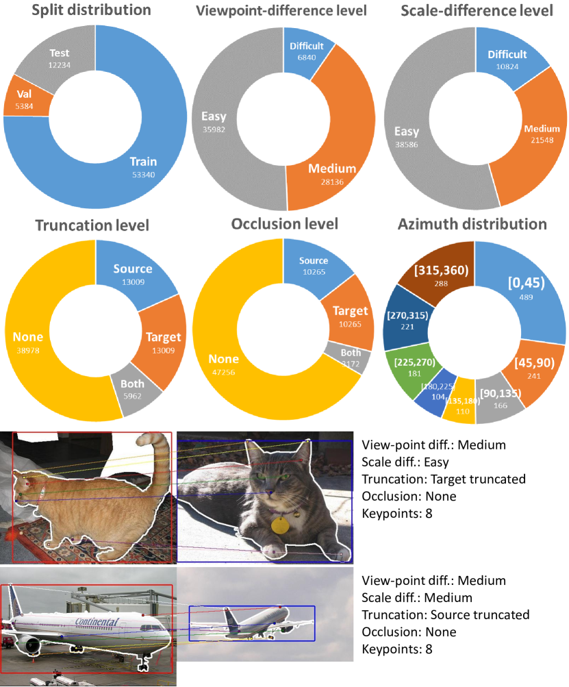
Figure 1: SPair-71k data statistics and example pairs with its annotations. Best viewed in electronic form.

Type	View-point diff.			Scale diff.			Truncation diff.				Occlusion diff.
	easy	medi	hard	easy	medi	hard	none	src	tgt	both	none	src	tgt	both
Train	26,466	21,646	5,228	29,248	16,184	7,908	29,184	9,796	9,796	4,564	35,330	7,737	7,737	2,536
Val	2,862	2,016	506	2,880	1,570	934	2,744	1,047	1,047	546	3,760	722	722	180
Test	6,654	4,474	1,106	6,458	3,794	1,982	7,050	2,166	2,166	852	8,166	1,806	1,806	456
All	35,982	28,136	6,840	38,586	21,548	10,824	38,978	13,009	13,009	5,962	47,256	10,265	10,265	3,172

Table 1: Distribution of SPair-71k in terms of difficulty labels.

Category	Train	Val	Test	All
aeroplane	2,924	304	690	3,918
bicycle	2,946	334	650	3,930
bird	3,080	272	702	4,054
boat	2,936	302	702	3,940
bottle	2,448	374	870	3,692
bus	2,708	250	644	3,602
car	2,960	274	564	3,798
cat	3,306	272	600	4,178
chair	3,060	306	646	4,012
cow	3,118	272	640	4,030
dog	3,192	306	600	4,098
horse	3,136	306	600	4,042
motorbike	3,180	238	702	4,120
person	3,066	306	650	4,022
potted plant	2,446	380	862	3,688
sheep	3,140	240	664	4,044
train	2,752	342	756	3,850
tv/monitor	2,942	306	692	3,940
total	53,340	5,384	12,234	70,958

Table 2: Distribution of SPair-71k in terms of category labels.

All previous datasets, however, have several drawbacks: First, the amount of data is not sufficient to train and test a large model. Second, image pairs do not display much variability in viewpoint, scale, occlusion, and truncation. Third, the annotations are often limited to either keypoints or object segmentation masks, which hinders in-depth analysis. Fourth, the datasets have no clear splits for training, validation, and testing. Due to this, recent evaluations in [5, 10, 11] have been done with different dataset splits of PF-PASCAL. Furthermore, the splits are disjoint in terms of image pairs, but not images: some images are shared between training and testing data.

To resolve these issues, we introduce a new dataset, SPair-71k, consisting of total 70,958 pairs of images from PASCAL 3D+ [14] and PASCAL VOC 2012 [2]. The dataset is significantly larger with rich annotations and clearly organized for learning. In particular, several types of useful annotations are available: keypoints of semantic parts, object segmentation masks, bounding boxes, view-point, scale, truncation, and occlusion differences for image pairs, etc. Figure 1 shows the dataset statistics in pie chart forms and sample image pairs with their annotations. Our benchmark is available online at http://cvlab.postech.ac.kr/research/SPair-71k/.

^∗This article is extended from section 4 of our recent paper [8] to provide the details of the dataset and more results.

Methods		aero	bike	bird	boat	bottle	bus	car	cat	chair	cow	dog	horse	moto	person	plant	sheep	train	tv	All
Authors’ original models	CNNGeo${}_{\textrm{res101}}$ [9]	21.3	15.1	34.6	12.8	31.2	26.3	24.0	30.6	11.6	24.3	20.4	12.2	19.7	15.6	14.3	9.6	28.5	28.8	18.1
	A2Net${}_{\textrm{res101}}$ [12]	20.8	17.1	37.4	13.9	33.6	29.4	26.5	34.9	12.0	26.5	22.5	13.3	21.3	20.0	16.9	11.5	28.9	31.6	20.1
	WeakAlign${}_{\textrm{res101}}$ [10]	23.4	17.0	41.6	14.6	37.6	28.1	26.6	32.6	12.6	27.9	23.0	13.6	21.3	22.2	17.9	10.9	31.5	34.8	21.1
	NC-Net${}_{\textrm{res101}}$ [11]	24.0	16.0	45.0	13.7	35.7	25.9	19.0	50.4	14.3	32.6	27.4	19.2	21.7	20.3	20.4	13.6	33.6	40.4	26.4
	HPFres50 [8]	25.3	18.5	47.6	14.6	37.0	22.9	18.3	51.1	16.7	31.5	30.8	19.1	23.7	23.8	23.5	14.4	30.8	37.2	27.2
	HPFres101 [8]	25.2	18.9	52.1	15.7	38.0	22.8	19.1	52.9	17.9	33.0	32.8	20.6	24.4	27.9	21.1	15.9	31.5	35.6	28.2
SPair-71k finetuned models	CNNGeo${}_{\textrm{res101}}$ [9]	23.4	16.7	40.2	14.3	36.4	27.7	26.0	32.7	12.7	27.4	22.8	13.7	20.9	21.0	17.5	10.2	30.8	34.1	20.6
	A2Net${}_{\textrm{res101}}$ [12]	22.6	18.5	42.0	16.4	37.9	30.8	26.5	35.6	13.3	29.6	24.3	16.0	21.6	22.8	20.5	13.5	31.4	36.5	22.3
	WeakAlign${}_{\textrm{res101}}$ [10]	22.2	17.6	41.9	15.1	38.1	27.4	27.2	31.8	12.8	26.8	22.6	14.2	20.0	22.2	17.9	10.4	32.2	35.1	20.9
	NC-Net${}_{\textrm{res101}}$ [11]	17.9	12.2	32.1	11.7	29.0	19.9	16.1	39.2	9.9	23.9	18.8	15.7	17.4	15.9	14.8	9.6	24.2	31.1	20.1

Table 3: Per-class PCK ($\alpha_{\text{bbox}}=0.1$) results on SPair-71k dataset. For the authors’ original models, the models of [9, 12] trained on PASCAL-VOC with self-supervision,  [10, 11] trained on PF-PASCAL with weak-supervision, and  [8] tuned using validation split of SPair-71k are used for evaluation. For SPair-71k-finetuned models, the original models are further finetuned on SPair-71k dataset by ourselves with our best efforts. Numbers in bold indicate the best performance and underlined ones are the second and third best.

Methods		View-point			Scale			Truncation				Occlusion				All
		easy	medi	hard	easy	medi	hard	none	src	tgt	both	none	src	tgt	both
Identity mapping		7.3	3.7	2.6	7.0	4.3	3.3	6.5	4.8	3.5	5.0	6.1	4.0	5.1	4.6	5.6
Authors’ original models	CNNGeo${}_{\textrm{res101}}$ [9]	25.2	10.7	5.9	22.3	16.1	8.5	21.1	12.7	15.6	13.9	20.0	14.9	14.3	12.4	18.1
	A2Net${}_{\textrm{res101}}$ [12]	27.5	12.4	6.9	24.1	18.5	10.3	22.9	15.2	17.6	15.7	22.3	16.5	15.2	14.5	20.1
	WeakAlign${}_{\textrm{res101}}$ [10]	29.4	12.2	6.9	25.4	19.4	10.3	24.1	16.0	18.5	15.7	23.4	16.7	16.7	14.8	21.1
	NC-Net${}_{\textrm{res101}}$ [11]	34.0	18.6	12.8	31.7	23.8	14.2	29.1	22.9	23.4	21.0	29.0	21.1	21.8	19.6	26.4
	HPFres50 [8]	35.0	18.9	13.6	32.0	25.1	15.4	29.7	24.5	23.5	22.9	29.6	22.9	22.1	21.3	27.2
	HPFres101 [8]	35.6	20.3	15.5	33.0	26.1	15.8	31.0	24.6	24.0	23.7	30.8	23.5	22.8	21.8	28.2
SPair-71k finetuned models	CNNGeo${}_{\textrm{res101}}$ [9]	28.8	12.0	6.4	24.8	18.7	10.6	23.7	15.5	17.9	15.3	22.9	16.1	16.4	14.4	20.6
	A2Net${}_{\textrm{res101}}$ [12]	30.9	13.3	7.4	26.1	21.1	12.4	25.0	17.4	20.5	17.6	24.6	18.6	17.2	16.4	22.3
	WeakAlign${}_{\textrm{res101}}$ [10]	29.3	11.9	7.0	25.1	19.1	11.0	24.0	15.8	18.4	15.6	23.3	16.1	16.4	15.7	20.9
	NC-Net${}_{\textrm{res101}}$ [11]	26.1	13.5	10.1	24.7	17.5	9.9	22.2	17.1	17.5	16.8	22.0	16.3	16.3	15.2	20.1

Table 4: PCK analysis by variation factors on SPair-71k. The variation factors include view-point, scale, truncation, and occlusion.

2 Dataset generation and annotation

We have created the SPair-71k dataset using 1,800 images from 18 categories of PASCAL VOC [2]. Specifically, we extract 1,000 images from 10 rigid categories of PASCAL 3D+ [14] (aeroplane, bike, boat, bottle, bus, car, chair, motorbike, train, tv/monitor) and 800 images of 8 non-rigid categories of PASCAL VOC 2012 [2] (bird, cat, cow, dog, horse, person, potted plant, sheep). Note that we do not use ‘dining table’ and ‘sofa’ categories present in PASCAL VOC as they usually appear as background and their semantic keypoints are too ambiguous to localize properly. The images are selected to cover diverse viewpoints of each category as much as possible. For the selected 1,800 images, we manually annotated keypoints and generate 70,958 pairs of images with pair-level annotations as follows.

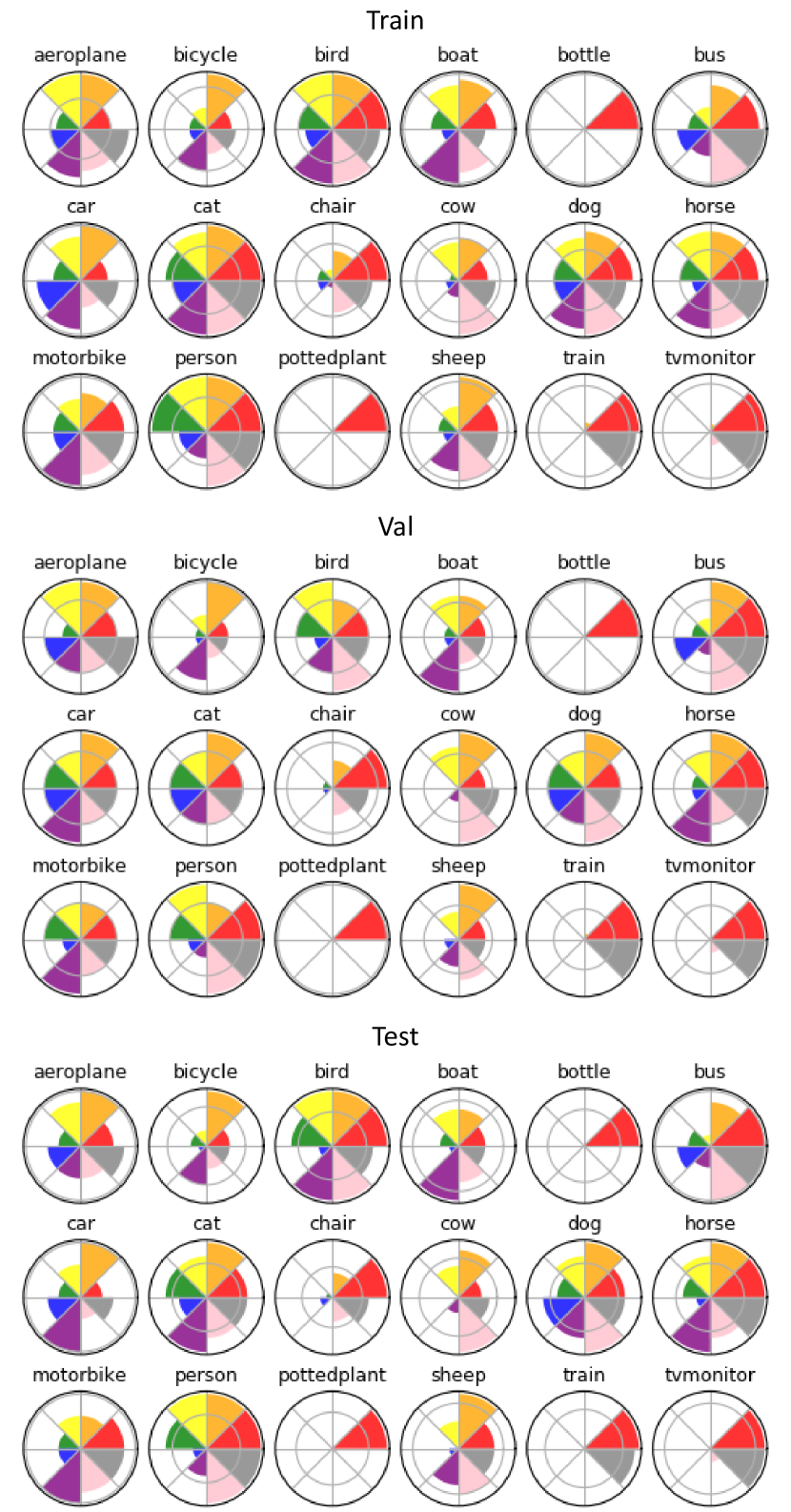
Figure 2: Azimuth distributions of SPair-71k training (top), validation (middle), and testing (bottom) images.

Image-level annotations. Keypoints for each object category are carefully selected and annotated according to three keypoint selection criteria: (1) each keypoint should describe an object’s part shared across instances of the same object category, (2) keypoints of an object category should be distinct from each other, and (3) keypoints of an object category should spread over the whole object. The number of selected keypoints varies from 9 (potted plant) to 30 (car) across categories; occluded or truncated keypoints are not annotated, thus varying from 3 to 30 across instances in practice. Azimuths for 10 rigid categories are directly obtained from PASCAL 3D+ [14] and quantized to one of the eight angular bins while azimuth bins for the other 8 non-rigid categories are manually annotated. Bounding box, segmentation mask, truncation and occlusion labels are retrieved from PASCAL VOC 2012 [2] where both truncation and occlusion labels are binary indicators, i.e., whether an instance in the image is truncated (occluded) or not.

Image-level splits. In order to build disjoint splits of image pairs for training, validation, and testing, we first create corresponding splits of images before generating pairs. 100 images of each object category are divided into three splits with an approximate ratio of 5:2:3 so that the images of each split spreads over quantized azimuth values, thus obtaining 997, 322, and 481 images for training, validation, and testing splits, respectively. Figure 2 shows category-wise circular histograms of azimuth values for the splits. Images of each split are then used to generate image pairs with pair-level annotations as follows.

Pair-level annotations. We build pair-level annotations using keypoints, azimuth bins, bounding boxes, truncations, and occlusions annotated in images. Common keypoints in two images are used as keypoints of pair-level annotations, i.e., keypoint correspondences. If there are no common keypoints between the two, the pair is excluded. View-point differences are divided into three levels of ‘easy’, ‘medium’, and ‘hard’; a pair is marked as ‘easy’, ‘medium’, and ‘hard’ if the difference between azimuth bin indexes of the two instances falls in the range of {0, 1}, {2, 3}, and {4}, respectively. Scale differences are labeled levels of ‘easy’, ‘medium’, and ‘hard’; a pair is labeled ‘easy’, ‘medium’, and ‘hard’ if the area ratio of corresponding object bounding boxes falls in the range of [1,2), [2, 4), [4, $\infty$]. Each pair is also annotated for both truncation and occlusion levels with ‘none’, ‘source only’, ‘target only’, and ‘both’. See Table 1 and 2 for details.

Finally, we obtain the SPair-71k dataset of 70,958 image pairs in total, which consists of 53,340 for training, 5,384 for validation, and 12,234 for testing, respectively.

Approach	Methods	View-point			Scale			Truncation				Occlusion				All
		easy	medi	hard	easy	medi	hard	none	src	tgt	both	none	src	tgt	both
Image alignment	CNNGeo${}_{\textrm{res101}}$ [9]	44.3	15.1	9.9	44.3	31.0	16.5	44.3	28.4	32.6	26.2	44.3	31.3	31.6	20.9	20.6
	A2Net${}_{\textrm{res101}}$ [12]	45.0	15.8	10.4	45.0	34.2	18.6	45.0	32.5	36.4	30.0	45.0	32.3	29.7	24.0	22.3
	WeakAlign${}_{\textrm{res101}}$ [10]	44.8	15.3	10.2	44.8	32.0	17.1	44.8	29.2	33.9	26.1	44.8	31.5	31.1	24.6	20.9
Region matching	NC-Net${}_{\textrm{res101}}$ [11]	49.8	23.4	19.1	49.8	35.7	19.6	49.8	33.7	36.8	33.8	49.8	35.6	35.9	27.4	26.4
	HPFres50 [8]	50.1	22.8	21.1	50.1	35.6	23.0	50.1	37.4	36.0	33.1	50.1	36.7	35.6	28.8	27.2
	HPFres101 [8]	51.0	25.2	23.8	51.0	37.3	22.8	51.0	36.7	36.8	33.1	51.0	37.6	36.7	29.6	28.2

Table 5: PCK analysis by controlling individual variations. For each variation of view-point, scale, truncation, and occlusion, the difficulty levels of the other variations are fixed as easy (view-point and scale) and none (truncation and occlusion). In this experiment, we use author’s original models for [8, 10, 11] and SPair-71k-finetuned models for [9, 12] in favor of better performance.

3 Baseline results on SPair-71k

We evaluate recent state-of-the-art methods [8, 9, 10, 11, 12] on SPair-71k to provide baseline results for further research. For each method in comparison, we run two versions of each model: an original trained model provided by the authors and a model further finetuned by ourselves using SPair-71k train/val set. The results are shown in Table 3. We fail to successfully train the method of [10, 11] on SPair-71k so that their performances drop when trained. We guess that their original learning objectives for weakly-supervised learning is fragile in presence of large view-point differences as in SPair-71k. We leave this issue for further investigation and will update the results at our benchmark page.

Analysis by variation factors. Each image pair in SPair-71k has annotations of difficulty levels for four variation factors (i.e., view-point, scale, truncation, and occlusion) between corresponding instances of the same category; ‘easy’, ‘medium’, or ‘hard’ is annotated for view-point and scale changes, while ‘none’, ‘source’, ‘target’ or ‘both’ is annotated for truncation and occlusion. PCK analysis of the models using these annotations are summarized in Table 4. The results show that all the models perform better given pairs with less variation, and that view-point and scale changes significantly affect the performances.

Impact of individual variations. The results in Table 4 does not clearly demonstrate an impact of each individual variation because the four types of variations co-exist in a pair and interfere with each other when evaluated. To measure an impact of each variation individually, we need to control the other variations to remain fixed. To this end, we evaluate the performances of different levels of a specific variation factor while fixing the levels of the other variations as easy (view-point and scale) and none (truncation and occlusion). For example, when evaluating the performances varying view-point levels, we only use pairs that are labeled ‘easy’ scale, ‘none’ truncation, and ‘none’ occlusion. The results are summarized in Table 5. It shows that the performances of local-region-matching methods [8, 11] is more robust to view-point variation compared to global-image-alignment methods [9, 10, 12]; the performance of the image alignment models drops more quickly than those of the region matching ones. In terms of scale changes, truncation, and occlusion, however, we find no significant difference in performance drop between the methods. While both truncation and occlusion clearly degrade the performances, the impacts are less than view-point and scale variations.

4 Conclusion

In this paper, we have presented a large-scale benchmark dataset, SPair-71k, which consists of 71k image pairs for semantic correspondence. Compared to previous datasets, it contains a significantly large number of image pairs with diverse variations in view-point, scale, truncation and occlusion, thus generalizing the problem of visual correspondence by reflecting real-world scenarios. Moreover, its rich annotations including object bounding boxes, keypoint correspondences, variation factors, azimuths, and object segmentation masks will be useful for future research on semantic correspondence and its joint problems.

Acknowledgements. This work is supported by Samsung Advanced Institute of Technology (SAIT) and Basic Science Research Program (NRF-2017R1E1A1A01077999), and also in part by the Inria/NYU collaboration and the Louis Vuitton/ENS chair on artificial intelligence.

References

- [1] Xianjie Chen, Roozbeh Mottaghi, Xiaobai Liu, Sanja Fidler, Raquel Urtasun, and Alan Yuille. Detect what you can: Detecting and representing objects using holistic models and body parts. In Proc. IEEE Conference on Computer Vision and Pattern Recognition (CVPR), 2014.
- [2] Mark Everingham, S. M. Ali Eslami, Luc Van Gool, Christopher K. I. Williams, John Winn, and Andrew Zisserman. The pascal visual object classes challenge: A retrospective. International Journal of Computer Vision (IJCV), 111(1):98–136, Jan 2015.
- [3] Bumsub Ham, Minsu Cho, Cordelia Schmid, and Jean Ponce. Proposal flow. In Proc. IEEE Conference on Computer Vision and Pattern Recognition (CVPR), pages 3475–3484, 2016.
- [4] Bumsub Ham, Minsu Cho, Cordelia Schmid, and Jean Ponce. Proposal flow: Semantic correspondences from object proposals. IEEE Transactions on Pattern Analysis and Machine Intelligence (TPAMI), 40(7):1711–1725, 2018.
- [5] Kai Han, Rafael S Rezende, Bumsub Ham, Kwan-Yee K Wong, Minsu Cho, Cordelia Schmid, and Jean Ponce. Scnet: Learning semantic correspondence. In Proc. IEEE International Conference on Computer Vision (ICCV), 2017.
- [6] Jaechul Kim, Ce Liu, Fei Sha, and Kristen Grauman. Deformable spatial pyramid matching for fast dense correspondences. In Proc. IEEE Conference on Computer Vision and Pattern Recognition (CVPR), pages 2307–2314, 2013.
- [7] Ce Liu, Jenny Yuen, and Antonio Torralba. Sift flow: Dense correspondence across scenes and its applications. In Proc. European Conference on Computer Vision (ECCV), 2008.
- [8] Juhong Min, Jongmin Lee, Jean Ponce, and Minsu Cho. Hyperpixel flow: Semantic correspondence with multi-layer neural features. In Proc. IEEE International Conference on Computer Vision (ICCV), 2019.
- [9] Ignacio Rocco, Relja Arandjelovic, and Josef Sivic. Convolutional neural network architecture for geometric matching. In Proc. IEEE Conference on Computer Vision and Pattern Recognition (CVPR), 2017.
- [10] Ignacio Rocco, Relja Arandjelović, and Josef Sivic. End-to-end weakly-supervised semantic alignment. In Proc. IEEE Conference on Computer Vision and Pattern Recognition (CVPR), 2018.
- [11] Ignacio Rocco, Mircea Cimpoi, Relja Arandjelović, Akihiko Torii, Tomas Pajdla, and Josef Sivic. Neighbourhood consensus networks. In Proc. Neural Information Processing Systems (NeurIPS), pages 1656–1667, 2018.
- [12] Paul Hongsuck Seo, Jongmin Lee, Deunsol Jung, Bohyung Han, and Minsu Cho. Attentive semantic alignment with offset-aware correlation kernels. In Proc. European Conference on Computer Vision (ECCV), 2018.
- [13] Tatsunori Taniai, Sudipta N Sinha, and Yoichi Sato. Joint recovery of dense correspondence and cosegmentation in two images. In Proc. IEEE Conference on Computer Vision and Pattern Recognition (CVPR), pages 4246–4255, 2016.
- [14] Yu Xiang, Roozbeh Mottaghi, and Silvio Savarese. Beyond pascal: A benchmark for 3d object detection in the wild. Proc. Winter Conference on Applications of Computer Vision (WACV), pages 75–82, 2014.