Semiclassical inverse spectral problem for elastic Love waves in isotropic media

Abstract

We analyze the inverse spectral problem on the half line associated with elastic surface waves. Here, we focus on Love waves. Under certain generic conditions, we establish uniqueness and present a reconstruction scheme for the S- wavespeed with multiple wells from the semiclassical spectrum of these waves.

1 Introduction

We analyze the inverse spectral problem on the half line associated with elastic surface waves. Here, we focus on Love waves. In a follow-up paper we present the corresponding inverse problem for Rayleigh waves. Surface waves have played a key role in revealing Earth’s structure from the shallow near-surface to several hundred kilometers deep into the mantle, depending on the frequencies and data acquisition configurations considered.

1.1 Seismology

The inverse spectral problem for surface waves fits in the seismological framework of surface-wave tomography. Surface-wave tomography has a long history. Since pioneering work on inference from the dispersion of surface waves half a century ago [15, 26, 4, 18, 34, 32, 13, 36, 24], surface wave tomography based on dispersion of waveforms from earthquake data has played an important role in studies of the structure of the Earth’s crust and upper mantle on both regional and global scales [20, 37, 23, 25, 22, 35, 14, 27, 33, 3, 28, 19, 40].

In order to avoid the effects of scattering due to complex crustal structure, these studies focused on the analysis, measurement, and inversion of surface wave dispersion at relatively low frequencies (that is, $4-20$ mHz, or periods between $50$ to $250$ s) at which the fundamental modes sense mantle structure to $200-300$ km depth and higher modes reach across the upper mantle and transition zone to some $660$ km depth. Most methods assume some form of (WKB) asymptotic and path-average approximation [9] in line with our semiclassical point of view.

More than a decade ago, Campillo and his collaborators discovered that cross correlation of ambient noise yields Green’s function for surface waves [11, 30, 31]. This enabled the possibility to extend the applicability of surface-wave tomography not only to any area where seismic sensors can be placed, but also to short-path measurements and frequencies at which the data are most sensitive to shallow depths. Crustal studies based on ambient noise tomography are typically conducted in the period band of $5–40$ s, but shorter period surface waves ($\sim 1$ s, using station spacing of $\sim 20$ km or less) have been used to investigate shallow crustal or even near surface shear-wave speed variations [29, 39, 40, 38, 21, 17].

1.2 Semiclassical analysis perspective

In a separate contribution [10], we presented the semiclassical analysis of surface waves. Such an analysis leads to a geometric-spectral description of the propagation of these waves [1, 36]. This semiclassical analysis is built on the work of Colin de Verdière [6, 7]. The main contribution of this paper is the construction of the Bohr-Sommerfeld quantization for Love waves. Colin de Verdière also considered the inverse spectral problem of scalar surface waves allowing wavespeed profiles that contain a well [8]. His result does not account for the Neumann boundary condition at the surface, although a reflection principle could be invoked, but his methodology directly applies once the Bohr-Sommerfeld quantization is obtained. The reflection principle does not apply to general elastic surface waves and the remedy is presented in this paper. In the process, we show that with the Neumann boundary condition at the surface, in fact, ambiguities arising in the recovery of the S-wave speed on the line (that is, without this boundary condition) can be resolved.

We study the elastic wave equation in $X={\mathbb{R}}^{2}\times(-\infty,0]$. In coordinates,

$$(x,z),\quad x=(x_{1},x_{2})\in{\mathbb{R}}^{2},\ z\in{\mathbb{R}}^{-}=(-\infty,0],$$

we consider solutions, $u=(u_{1},u_{2},u_{3})$, satisfying the Neumann boundary condition at $\partial X=\{z=0\}$, to the system

(1) $$\begin{split}\partial^{2}_{t}u_{i}+M_{il}u_{l}&=0,\\ u(t=0,x,z)&=0,~{}~{}\partial_{t}u(t=0,x,z)=h(x,z),\\ \frac{c_{i3kl}}{\rho}\partial_{k}u_{l}(t,x,z=0)&=0,\end{split}$$

where

$$M_{il}=-\frac{\partial}{\partial z}\frac{c_{i33l}(x,z)}{\rho(x,z)}\frac{\partial}{\partial z}-\sum_{j,k=1}^{2}\frac{c_{ijkl}(x,z)}{\rho(x,z)}\frac{\partial}{\partial x_{j}}\frac{\partial}{\partial x_{k}}-\sum_{j=1}^{2}\frac{\partial}{\partial x_{j}}\frac{c_{ij3l}(x,z)}{\rho(x,z)}\frac{\partial}{\partial z}\\ -\sum_{k=1}^{2}\frac{c_{i3kl}(x,z)}{\rho(x,z)}\frac{\partial}{\partial z}\frac{\partial}{\partial x_{k}}-\sum_{k=1}^{2}\left(\frac{\partial}{\partial z}\frac{c_{i3kl}(x,z)}{\rho(x,z)}\right)\frac{\partial}{\partial x_{k}}-\sum_{j,k=1}^{2}\left(\frac{\partial}{\partial x_{j}}\frac{c_{ijkl}(x,z)}{\rho(x,z)}\right)\frac{\partial}{\partial x_{k}}.$$

Here, the stiffness tensor, $c_{ijkl}$, and density, $\rho$, are smooth and obey the following scaling: Introducing $Z=\frac{z}{\epsilon}$,

$$\frac{c_{ijkl}}{\rho}(x,z)=C_{ijkl}\left(x,\frac{z}{\epsilon}\right),~{}~{}\epsilon\in(0,\epsilon_{0}];$$

$$C_{ijkl}(x,Z)=C_{ijkl}(x,Z_{I})=C_{ijkl}^{I}(x),\quad Z\leq Z_{I}<0.$$

As discussed in [10], surface waves travel along the surface $z=0$.

The remainder of the paper is organized as follows. In Section 2, we give the formulation of the inverse problems as an inverse spectral problem on the half line. In Section 3, we treat the simple case of recovery of a monotonic profile of wave speed. In Section 4, we discuss the relevant Bohr-Sommerfeld quantization, which is the corner stone in the study of the inverse spectral problem. In Section 5, we give the reconstruction scheme under generic assumptions.

2 Semiclassical description of Love waves

2.1 Surface wave equation, trace and the data

For the convenience of the readers, we briefly summarize the semiclassical description of elastic surface waves. The leading-order Weyl symbol associated with $M_{il}$ above is given by

(2) $$H_{0,il}(x,\xi)=-\frac{\partial}{\partial Z}C_{i33l}(x,Z)\frac{\partial}{\partial Z}\\ -\mathrm{i}\sum_{j=1}^{2}C_{ij3l}(x,Z)\xi_{j}\frac{\partial}{\partial Z}-\mathrm{i}\sum_{k=1}^{2}C_{i3kl}(x,Z)\frac{\partial}{\partial Z}\xi_{k}-\mathrm{i}\sum_{k=1}^{2}\left(\frac{\partial}{\partial Z}C_{i3kl}(x,Z)\right)\xi_{k}\\ +\sum_{j,k=1}^{2}C_{ijkl}(x,Z)\xi_{j}\xi_{k}.\hskip 113.81102pt$$

We view $H_{0}(x,\xi)$ as ordinary differential operators in $Z$, with domain

$$\mathcal{D}=\left\{v\in H^{2}(\mathbb{R}^{-})\ \bigg{|}\ \sum_{l=1}^{3}\left(C_{i33l}(x,0)\frac{\partial v_{l}}{\partial Z}(0)+\mathrm{i}\sum_{k=1}^{2}C_{i3kl}\xi_{k}v_{l}(0)\right)=0\right\}.$$

For an isotropic medium,

$$C_{ijkl}=\hat{\lambda}\delta_{ij}\delta_{kl}+\hat{\mu}(\delta_{ik}\delta_{jl}+\delta_{il}\delta_{jk}),$$

where $\hat{\lambda}=\frac{\lambda}{\rho}$ and $\hat{\mu}=\frac{\mu}{\rho}$. The S-wavespeed, $C_{S}$, is then $C_{S}=\sqrt{\hat{\mu}}$. The decoupling of Love and Rayleigh waves is observed in practice, and explained in [10]. We denote

$$P(\xi)=\left(\begin{array}[]{ccc}|\xi|^{-1}\xi_{2}&|\xi|^{-1}\xi_{1}&0\\ -|\xi|^{-1}\xi_{1}&|\xi|^{-1}\xi_{2}&0\\ 0&0&1\end{array}\right).$$

Then

$$P(\xi)^{-1}H_{0}(x,\xi)P(\xi)=\left(\begin{array}[]{cc}H_{0}^{L}(x,\xi)&\\ &H_{0}^{R}(x,\xi)\end{array}\right),$$

where

(3) $$H_{0}^{L}(x,\xi)\varphi_{1}=-\frac{\partial}{\partial Z}\hat{\mu}\frac{\partial\varphi_{1}}{\partial Z}+\hat{\mu}\,|\xi|^{2}\varphi_{1}$$

supplemented with boundary condition

$$\frac{\partial\varphi_{1}}{\partial Z}(0)=0,$$

for Love waves. We will consider only the Love waves in this paper.

We assume that $\Lambda_{\alpha}(x,\xi)$ is an eigenvalue of $H_{0}(x,\xi)$ with eigenfunction $\Phi_{\alpha,0}(Z,x,\xi)$. By [10, Theorem 2.1], we have

(4) $$H_{0}^{L}\circ\Phi_{\alpha,0}\,=\Phi_{\alpha,0}\circ\Lambda_{\alpha}+\mathcal{O}(\epsilon).$$

We define

(5) $$J_{\alpha,\epsilon}(Z,x,\xi)=\frac{1}{\sqrt{\epsilon}}\Phi_{\alpha,0}(Z,x,\xi).$$

Microlocally (in $x$), we can construct approximate solutions of the system (1) with initial values

$$h(x,\epsilon Z)=\sum_{\alpha=1}^{\mathfrak{M}}J_{\alpha,\epsilon}(Z,x,\epsilon D_{x})W_{\alpha,\epsilon}(x,Z),$$

representing surface waves. We assume that all eigenvalues $\Lambda_{1}<\cdots<\Lambda_{\alpha}<\cdots<\Lambda_{\mathfrak{M}}$ are eigenvalues of the operator given in (3). We let $W_{\alpha,\epsilon}$ solve the initial value problems (up to leading order)

(6) $$[\epsilon^{2}\partial_{t}^{2}+\Lambda_{\alpha}(x,D_{x})]W_{\alpha,\epsilon}(t,x,Z) = 0,$$

(7) $$W_{\alpha,\epsilon}(0,x,Z) = 0,\quad\partial_{t}W_{\alpha,\epsilon}(0,x,Z)=J_{\alpha,\epsilon}W_{\alpha}(x,Z),$$

$\alpha=1,\ldots,\mathfrak{M}$. We let $\mathcal{G}_{0}(Z,x,t,Z^{\prime},\xi;\epsilon)$ denote the approximate Green’s function (microlocalized in $x$), up to leading order, for Love waves. We may write [10]

(8) $$\mathcal{G}_{0}(Z,x,t,Z^{\prime},\xi;\epsilon)=\sum_{\alpha=1}^{\mathfrak{M}}J_{\alpha,\epsilon}(Z,x,\xi)\\ \left(\frac{\mathrm{i}}{2}\mathcal{G}_{\alpha,+,0}(x,t,\xi,\epsilon)-\frac{\mathrm{i}}{2}\mathcal{G}_{\alpha,-,0}(x,t,\xi,\epsilon)\right)\Lambda^{-1/2}_{\alpha}(x,\xi)J_{\alpha,\epsilon}(Z^{\prime},x,\xi),$$

where $\mathcal{G}_{\alpha,\pm,0}$ are Green’s functions for half wave equations associated with (6)-(7). We have the trace

$$\int_{\mathbb{R}^{-}}\widehat{\epsilon\partial_{t}\mathcal{G}_{0}}(Z,x,\omega,Z,\xi;\epsilon)\mathrm{d}\epsilon Z=\sum_{\alpha=1}^{\mathfrak{M}}\delta(\omega^{2}-\Lambda_{\alpha}(x,\xi))\Lambda^{1/2}_{\alpha}(x,\xi)+{\mathcal{O}}(\epsilon^{-1})$$

from which we can extract the eigenvalues $\Lambda_{\alpha},\,\alpha=1,2,\cdots,\mathfrak{M}$ as functions of $\xi$. We use these to recover the profile of $C_{S}^{2}$.

In practice, these eigenvalues are obtained from surface-wave tomography and to ensure that all eigenvalues are observed, measurements of surface-waveforms should be taken in boreholes. Most seismic observations are made at or near Earth’s surface, but modern networks increasingly include borehole sensors indeed. For example, Hi-net seismographic network in Japan includes more than $750$ sensors located in $>100$ m deep boreholes and permanent sites of USArray include sensors placed around $100$ m depth.

2.2 Semiclassical spectrum

From here on, we only consider the operator $H_{0}^{L}(x,\xi)$ for Love waves. We suppress the dependence on $x$, and introduce $h=|\xi|^{-1}$ as another semiclassical parameter. Within this setting, we also change the notation from $\frac{\partial}{\partial Z}$ to $\frac{\mathrm{d}}{\mathrm{d}Z}$. We arrive at the operator

$$L_{h}=-h^{2}\frac{\mathrm{d}}{\mathrm{d}Z}\left(\hat{\mu}(Z)\frac{\mathrm{d}}{\mathrm{d}Z}\right)+\hat{\mu}(Z)$$

with Neumann boundary condition at $Z=0$. The assumption on the stiffness tensor gives us the following assumption on $\hat{\mu}$:

Assumption 2.1.

The (unknown) function $\hat{\mu}$ satisfies $\hat{\mu}(Z)=\hat{\mu}(Z_{I})$ for all $Z\leq Z_{I}$ and

$$0<\hat{\mu}(0)=E_{0}=\inf_{Z\leq 0}\hat{\mu}(Z)<\hat{\mu}_{I}=\sup_{Z\leq 0}\hat{\mu}(Z)=\hat{\mu}(Z_{I}).$$

The assumption that $\hat{\mu}$ attains its mininum at the boundary, and its maximum in some deep zone, is realistic in practice.

We first observe that the spectrum of $L_{h}$ is divided in two parts,

$$\sigma(L_{h})=\sigma_{pp}(L_{h})\cup\sigma_{ac}(L_{h}),$$

where the point spectrum $\sigma_{pp}(L_{h})$ consists of a finite number of eigenvalues in $(E_{0},\hat{\mu}_{I})$ and the continuous spectrum $\sigma_{ac}(L_{h})=[\hat{\mu}_{I},\infty)$. We write $\lambda_{\alpha}=h^{2}\Lambda_{\alpha}$. Since this is a one-dimensional problem, the eigenvalues are simple and satisfy

$$E_{0}<\lambda_{1}(h)<\lambda_{2}(h)<\ldots<\lambda_{\mathfrak{M}}(h)<\hat{\mu}_{I};$$

the number of eigenvalues, $\mathfrak{M}$ increases as $h$ decreases.

We will study how to reconstruct the profile $\hat{\mu}$ using only the asymptotic behavior of $\lambda_{\alpha}(h)$ in $h$. To this end, we introduce the semiclassical spectrum as in [8]

Definition 1.

For given $E$ with $E_{0}<E\leq\hat{\mu}_{I}$ and positive real number $N$, a sequence $\mu_{\alpha}(h)$, $\alpha=1,2,\ldots$ is a semiclassical spectrum of $L_{h}$ mod $o(h^{N})$ in $]-\infty,E[$ if, for all $\lambda_{\alpha}(h)<E$,

$$\lambda_{\alpha}(h)=\mu_{\alpha}(h)+o(h^{N})$$

uniformly on every compact subset $K$ of $]-\infty,E[\,$.

3 Reconstruction of a monotonic profile

In this section, we give a reconstruction scheme for the simple situation where the profile $\hat{\mu}$ is monotonic. First it is well known that

Lemma 2.

The first eigenvalue of $L_{h}$ satisfies $\lim_{h\rightarrow 0}\lambda_{1}(h)=E_{0}$.

Similar to Theorem 3 in [6], we have

Theorem 3.

Assume that $\hat{\mu}$ is decreasing in $[Z_{I},0]$. Then the asymptotics of the discrete spectra $\lambda_{j}(h),$ $1\leq j\leq\mathfrak{M}_{j}$ as $h\to 0$ determine the function $\hat{\mu}$.

Before giving the proof, we recall the Abel transform and its inverse. We introduce

$$\mathcal{A}g(E)=\int_{E_{0}}^{E}\sqrt{E-u}g(u)\,\mathrm{d}u.$$

Then

$$\frac{\mathrm{d}}{\mathrm{d}E}\mathcal{A}g(E)=\frac{1}{2}Tg(E),\quad Tg(E)=\int_{E_{0}}^{E}\frac{g(u)}{\sqrt{E-u}}\,\mathrm{d}u,$$

where $Tg$ signifies the Abel transform of $g$. By the inversion formula for the Abel transform,

$$\frac{\mathrm{d}}{\mathrm{d}E}T^{2}g(E)=\pi g(E),$$

we get

(9) $$\left(\frac{4}{\pi}\frac{\mathrm{d}^{2}}{\mathrm{d}E^{2}}\mathcal{A}\frac{\mathrm{d}}{\mathrm{d}E}\mathcal{A}\right)g(E)=g(E).$$

Proof.

First, we note that $E_{0}=\hat{\mu}(0)$ is determined by the first semiclassical eigenvalue $\lambda_{1}(h)$ by Lemma 2. Then, we invoke Weyl’s law. For $E<\hat{\mu}_{I}$, let $N(h,E)=\#\{\lambda_{j}(h)\leq E\}$, where $\lambda_{j}(h)$ is an eigenvalue for $L_{h}$. Then [10]

(10) $$N(h,E)=\frac{1}{2\pi h}\left[{\rm Area}(\{(Z,\zeta)\ :\ \hat{\mu}(Z)(1+\zeta^{2})\leq E\})+o(1)\right].$$

Thus, from the leading order behavior (in $h$) of $\lambda_{j}(h)$ we can recover

$${\rm Area}(\{(Z,\zeta)\ :\ \hat{\mu}(Z)(1+\zeta^{2})\leq E\})=2\tilde{S}^{1}_{0}(E),\quad\tilde{S}^{1}_{0}(E)=\int_{f(E)}^{0}\sqrt{\frac{E-\hat{\mu}}{\hat{\mu}}}\,\mathrm{d}Z,$$

with $\hat{\mu}(f(E))=E$. We change variable of integration, $Z=f(u)$, with

(11) $$\left.\frac{\mathrm{d}}{\mathrm{d}Z}\hat{\mu}(Z)\right|_{Z=f(u)}=\frac{1}{f^{\prime}(u)}$$

and get

$$\tilde{S}^{1}_{0}(E)=\mathcal{A}g(E),\quad g(u)=\frac{f^{\prime}(u)}{\sqrt{u}}.$$

Applying (9) above, we recover $g$, that is,

$$f^{\prime}(E)=\left(\frac{4}{\pi}\sqrt{E}\frac{\mathrm{d}^{2}}{\mathrm{d}E^{2}}\mathcal{A}\frac{\mathrm{d}}{\mathrm{d}E}\right)\tilde{S}^{1}_{0}(E),\quad E_{0}<E<\hat{\mu}_{I}.$$

Then

$$f(E)=\int_{E_{0}}^{E}f^{\prime}(u)\,\mathrm{d}u,$$

using that $f(E_{0})=0$ and knowledge of $E_{0}=\hat{\mu}(0)$ from the first eigenvalue (Lemma 2), from which we recover $\hat{\mu}$ by the inverse function theorem. ∎

4 Bohr-Sommerfeld quantization

The Bohr-Sommerfeld rules give a quantization for the semiclassical spectrum [5]. We will derive these rules making use of the WKB-Maslov Ansatz for the eigenfunctions. We obtain an alternative proof to the one given in [7, 8], which enables to explicitly incorporate Neumann boundary conditions at the surface. It opens the way for studying inverse problems also for Rayleigh waves; these will be investigated in a follow-up paper.

We construct WKB solutions of the form

(12) $$u_{h}(Z)=C\exp\left[\frac{1}{h}\sum_{j=0}^{\infty}h^{j}\mathcal{S}_{j}(Z)\right]$$

that satisfy

(13) $$-h^{2}\hat{\mu}(Z)u_{h}^{\prime\prime}(Z)-h^{2}\hat{\mu}^{\prime}(Z)u_{h}^{\prime}(Z)+\hat{\mu}(Z)u_{h}(Z)=Eu_{h}(Z).$$

We will follow various calculations from [2] in the following analysis.

4.1 Half well

We consider the eigenvalue problem on the half line $\mathbb{R}^{-}$, with Neumann boundary condition at $Z=0$. We fix a real number $E$ and assume that there exists a unique $Z_{E}$ such that $\hat{\mu}(Z_{E})=E$. For exposition of the construction, we change the variable $Z\rightarrow Z_{E}-Z$ such that $\hat{\mu}(0)=E$ and $Z_{E}$ is the boundary point. Furthermore, we assume that $\hat{\mu}(Z)-E>0$ for $Z>0$ and $\hat{\mu}(Z)-E<0$ for $Z_{E}<Z<0$. The original domain $]-\infty,0]$ changes to $[Z_{E},\infty[$. We divide the domain $[Z_{E},\infty[$ into three regions: region $\mathrm{I}$ $(Z>0)$, region $\mathrm{II}$ ($|Z|$ is small) and region $\mathrm{III}$ $(Z_{E}\leq Z<0)$. We will construct WKB solutions in each region and glue them together.

First, we construct the WKB solution, $u_{\mathrm{I}}(Z)$, in region I. We substitute solutions of the form (12), collect terms of equal orders in $h$, and arrive at an infinite family of equations which may be solved recursively. The $\mathcal{O}(h^{0})$ terms give the eikonal equation for $\mathcal{S}_{0}$,

$$\hat{\mu}(Z)(1-(\mathcal{S}_{0}^{\prime}(Z))^{2})=E.$$

We select the solution

(14) $$\mathcal{S}_{0}(Z)=-\int_{0}^{Z}\sqrt{\frac{\hat{\mu}-E}{\hat{\mu}}}\mathrm{d}Z^{\prime}.$$

Then the $\mathcal{O}(h)$ term yields

$$\hat{\mu}\mathcal{S}_{0}^{\prime\prime}+2\hat{\mu}\mathcal{S}_{0}^{\prime}\mathcal{S}_{1}^{\prime}+\hat{\mu}^{\prime}\mathcal{S}_{0}^{\prime}=0,$$

which implies that

$$\mathcal{S}_{1}^{\prime}=-\frac{1}{2}(\log(\hat{\mu}\mathcal{S}_{0}^{\prime}))^{\prime}=-\frac{1}{4}\left(\log[\hat{\mu}(\hat{\mu}-E)]\right)^{\prime};$$

we select the solution

(15) $$\mathcal{S}_{1}=-\frac{1}{4}\log[\hat{\mu}(\hat{\mu}-E)].$$

The lower order terms give us a sequence of equations,

$$2\hat{\mu}\mathcal{S}_{0}^{\prime}\mathcal{S}_{j}^{\prime}+(\hat{\mu}\mathcal{S}_{j-1}^{\prime})^{\prime}+\hat{\mu}\sum_{k=1}^{j-1}\mathcal{S}_{j-k}^{\prime}\mathcal{S}_{k}^{\prime}=0,\quad j\geq 2.$$

We write down the explicit form of $\mathcal{S}_{2}$ for later use

(16) $$\mathcal{S}_{2}(\delta,Z)=\int_{\delta}^{Z}\left[\frac{(E\hat{\mu}^{\prime}-2\hat{\mu}\hat{\mu}^{\prime})^{2}}{32\hat{\mu}^{3/2}(\hat{\mu}-E)^{5/2}}+\frac{-E^{2}\hat{\mu}^{\prime\prime}+3E\hat{\mu}\hat{\mu}^{\prime\prime}-2\hat{\mu}^{2}\hat{\mu}^{\prime\prime}+E(\hat{\mu}^{\prime})^{2}}{8(\hat{\mu}-E)^{5/2}\hat{\mu}^{1/2}}\right]\mathrm{d}Z^{\prime},$$

up to a constant difference; here $\delta$ is any small fixed positive constant. Upon integrating by parts, we obtain

(17) $$\begin{split}\mathcal{S}_{2}(\delta,Z)=-\frac{(3E+2\hat{\mu})\hat{\mu}^{\prime}}{48\hat{\mu}^{1/2}(\hat{\mu}-E)^{3/2}}-&\frac{\hat{\mu}^{\prime}}{24(\hat{\mu}-E)^{1/2}\hat{\mu}^{1/2}}\\ &+\int_{\delta}^{Z}\left[-\frac{(\hat{\mu}^{\prime})^{2}}{24\hat{\mu}^{3/2}(\hat{\mu}-E)^{1/2}}+\frac{(7E-8\hat{\mu})\hat{\mu}^{\prime\prime}}{48\hat{\mu}^{1/2}(\hat{\mu}-E)^{3/2}}\right]\mathrm{d}Z^{\prime}.\end{split}$$

Next, we consider region II containing the turning point. When $|Z|$ is small, we expand

$$\hat{\mu}(Z)-E=a_{1}Z+a_{2}Z^{2}+a_{3}Z^{3}+\cdots.$$

Here, $a_{1}>0$. We write $u_{\mathrm{II}}(Z)=\hat{\mu}^{-1/2}(Z)\,v_{\mathrm{II}}(Z)=(E+a_{1}Z+a_{2}Z^{2}+a_{3}Z^{3}+\cdots)^{-1/2}v_{\mathrm{II}}(Z)$. Then we obtain

$$-h^{2}\frac{\mathrm{d}}{\mathrm{d}Z}\left(\hat{\mu}\frac{\mathrm{d}u_{\mathrm{II}}}{\mathrm{d}Z}\right)=-h^{2}\frac{\mathrm{d}}{\mathrm{d}Z}\left(\hat{\mu}\frac{\mathrm{d}}{\mathrm{d}Z}\hat{\mu}^{-1/2}(Z)v_{\mathrm{II}}(Z)\right)=-h^{2}\hat{\mu}^{1/2}v_{\mathrm{II}}^{\prime\prime}+h^{2}(\hat{\mu}^{1/2})^{\prime\prime}v_{\mathrm{II}}.$$

Thus, by (13), we have the following equation for $v_{\mathrm{II}}$,

(18) $$h^{2}v_{\mathrm{II}}^{\prime\prime}=\left(1-E\hat{\mu}^{-1}+h^{2}\frac{(\hat{\mu}^{1/2})^{\prime\prime}}{\hat{\mu}^{1/2}}\right)\,v_{\mathrm{II}}.$$

We further employ the simple asymptotic expansion,

$$1-E\hat{\mu}^{-1}(Z)=b_{1}Z+b_{2}Z^{2}+\cdots,$$

where $b_{1}=\frac{a_{1}}{E}$ and $b_{2}=\frac{a_{2}E-a_{1}^{2}}{E^{2}}$. Temporarily, we introduce the scaling $Z=h^{2/3}b_{1}^{-1/3}Y$. With abuse of notation for $v_{\mathrm{II}}$, (18) gives

$$-h^{2}h^{-4/3}b_{1}^{2/3}\frac{\mathrm{d}^{2}v_{\mathrm{II}}}{\mathrm{d}Y^{2}}=(b_{1}h^{2/3}b_{1}^{-1/3}Y+b_{2}h^{4/3}b_{1}^{-2/3}Y^{2}+\cdots)\,v_{\mathrm{II}},$$

which can be simplified to

(19) $$\frac{\mathrm{d}^{2}v_{\mathrm{II}}}{\mathrm{d}Y^{2}}\sim(Y+h^{2/3}b_{1}^{-4/3}b_{2}Y^{2})\,v_{\mathrm{II}},$$

keeping the second-order approximation. We then seek an approximate solution of the form

$$v_{\mathrm{II}}(Y)\sim(1+\alpha_{1}h^{2/3}Y)\,\mathrm{Ai}(Y+\beta_{1}h^{2/3}Y^{2}),$$

where $\mathrm{Ai}$ is the Airy function and $\alpha_{1}$ and $\beta_{1}$ are constants to be determined. By tedious calculations, we find that

$$\frac{\mathrm{d}^{2}v_{\mathrm{II}}}{\mathrm{d}Y^{2}}\sim D\Big{[}\alpha_{1}h^{2/3}\mathrm{Ai}^{\prime}(Y+\beta_{1}h^{2/3}Y^{2})+\alpha_{1}h^{2/3}(1+2\beta_{1}h^{2/3}Y)\,\mathrm{Ai}^{\prime}(Y+\beta_{1}h^{2/3}Y^{2})\\ +(1+\alpha_{1}h^{2/3}Y)(1+2\beta_{1}h^{2/3}Y)^{2}\mathrm{Ai}^{\prime\prime}(Y+\beta_{1}h^{2/3}Y^{2})\\ +(1+\alpha_{1}h^{2/3}Y)\,2\beta_{1}h^{2/3}\mathrm{Ai}^{\prime}(Y+\beta_{1}h^{2/3}Y^{2})\Big{]}.$$

Comparing this equation with differential equation (19), and using that

$$\mathrm{Ai}^{\prime\prime}(Y+\beta_{1}h^{2/3}Y^{2})=(Y+\beta_{1}h^{2/3}Y^{2})\,\mathrm{Ai}(Y+\beta_{1}h^{2/3}Y^{2}),$$

we must have

$$\alpha_{1}+\beta_{1}=0,$$

and

$$5\beta_{1}=b^{-4/3}_{1}b_{2}.$$

Hence, undoing the scaling and returning to the original (depth) coordinate,

$$v_{\mathrm{II}}(Z)\sim D\left(1-\frac{b_{2}}{5b_{1}}Z\right)\,\mathrm{Ai}\left[b_{1}^{1/3}h^{-2/3}\left(Z+\frac{b_{2}Z^{2}}{5b_{1}}\right)\right]$$

so that

(20) $$u_{\mathrm{II}}(Z)\sim D\left(E^{-1/2}-\frac{1}{2}E^{-3/2}a_{1}Z\right)\\ \left(1-\frac{a_{2}E-a_{1}^{2}}{5Ea_{1}}Z\right)\mathrm{Ai}\left[\left(\frac{a_{1}}{E}\right)^{1/3}h^{-2/3}\left(Z+\frac{a_{2}E-a_{1}^{2}}{5Ea_{1}}Z^{2}\right)\right].$$

Now, we examine $u_{\mathrm{I}}(Z)$ for small $Z$. We make the following approximations

$$[\hat{\mu}(Z)(\hat{\mu}(Z)-E)]^{-1/4} \sim Z^{-1/4}(Ea_{1})^{-1/4}\left(1-\frac{1}{4}\frac{Ea_{2}+a_{1}^{2}}{Ea_{1}}Z\right),$$

$$\int_{0}^{Z}\sqrt{\frac{\hat{\mu}-E}{\hat{\mu}}}\mathrm{d}Z^{\prime} \sim \frac{2}{3}Z^{3/2}\left(\frac{a_{1}}{E}\right)^{1/2}+\frac{Ea_{2}-a_{1}^{2}}{5Ea_{1}}\left(\frac{a_{1}}{E}\right)^{1/2}Z^{5/2},$$

$$\mathcal{S}_{2}(\delta,Z) \sim -\frac{5}{48}E^{1/2}a_{1}^{-1/2}Z^{-3/2}-\frac{E^{1/2}a_{2}a_{1}^{-3/2}}{12}\delta^{-1/2}.$$

In the asymptotic expansion of $\mathcal{S}_{2}$, we neglect terms $\mathcal{O}(Z^{-1/2})$, which is justified because $hZ^{-1/2}$ is small (compared to $h\delta^{-1/2}$, $hZ^{-3/2}$) in the limit $h\to 0$. Substituting these formulas into $u_{\mathrm{I}}$ gives

$$u_{\mathrm{I}}\sim CZ^{-1/4}(Ea_{1})^{-1/4}\left(1-\frac{1}{4}\frac{Ea_{2}+a_{1}^{2}}{Ea_{1}}Z\right)\\ \exp\left[-\frac{2}{3h}Z^{3/2}\left(\frac{a_{1}}{E}\right)^{1/2}-\frac{1}{5h}\frac{Ea_{2}-a_{1}^{2}}{Ea_{1}}\left(\frac{a_{1}}{E}\right)^{1/2}Z^{5/2}\right.\\ \left.-\frac{h}{48}E^{1/2}a_{1}^{-5/2}Z^{-3/2}-\frac{h}{12}a^{-3/2}(2a_{1}-E)E^{-1/2}Z^{-3/2}-\frac{hE^{1/2}a_{2}a_{1}^{-3/2}}{12}\mu^{-1/2}\right].$$

Revisiting $u_{\mathrm{II}}(Z)$, for large positive $Z$, we employ the asymptotic behavior of $\mathrm{Ai}$,

$$\mathrm{Ai}(s)\sim\frac{1}{2\sqrt{\pi}}s^{-1/4}\left(1-\frac{5}{48}s^{-3/2}\right)\exp\left[-\frac{2}{3}s^{3/2}\right]$$

and obtain

$$u_{\mathrm{II}}(Z)\sim D\frac{1}{2\sqrt{\pi}}\left(\frac{a_{1}}{E}\right)^{-1/12}h^{1/6}Z^{-1/4}E^{-1/2}\left(1-\frac{Ea_{2}+a_{1}^{2}}{4Ea_{1}}Z\right)\\ \left(1-\frac{5}{48}hZ^{-3/2}\left(\frac{a_{1}}{E}\right)^{-1/2}\right)\exp\left[-\frac{2}{3}\left(\frac{a_{1}}{E}\right)^{1/2}h^{-1}Z^{3/2}\left(1+\frac{3}{2}\left(\frac{a_{2}E-a_{1}^{2}}{5Ea_{1}}\right)Z\right)\right].$$

Uniformly asymptotically matching $u_{\mathrm{I}}$ and $u_{\mathrm{II}}$ then leads to the condition,

(21) $$C=\frac{D}{2\sqrt{\pi}}h^{1/6}\exp\left[\frac{hE^{1/2}a_{2}a_{1}^{-3/2}}{12}\mu^{-1/2}\right]a_{1}^{1/6}E^{-1/3}.$$

In region III, we construct the (oscillatory) WKB solution,

(22) $$u_{\mathrm{III}}(Z)\sim F[(E-\hat{\mu})\hat{\mu}]^{-1/4}\exp\left[\frac{\mathrm{i}}{h}\mathcal{S}_{0}(Z)+\mathrm{i}h\mathcal{S}_{2}(\mu,Z)\right]\\ +G[(E-\hat{\mu})\hat{\mu}]^{-1/4}\exp\left[-\frac{\mathrm{i}}{h}\mathcal{S}_{0}(Z)-\mathrm{i}h\mathcal{S}_{2}(\mu,Z)\right],\quad\quad Z,h\rightarrow 0^{+},$$

where

(23) $$\mathcal{S}_{0}(Z)=\int_{Z}^{0}\sqrt{\frac{E-\hat{\mu}}{\hat{\mu}}}\mathrm{d}Z^{\prime}$$

and

(24) $$\mathcal{S}_{2}(\delta,Z)=-\int_{Z}^{-\delta}\left[\frac{(E\hat{\mu}^{\prime}-2\hat{\mu}\hat{\mu}^{\prime})^{2}}{32\hat{\mu}^{3/2}(E-\hat{\mu})^{5/2}}+\frac{-E^{2}\hat{\mu}^{\prime\prime}+3E\hat{\mu}\hat{\mu}^{\prime\prime}-2\hat{\mu}^{2}\hat{\mu}^{\prime\prime}+E(\hat{\mu}^{\prime})^{2}}{8(E-\hat{\mu})^{5/2}\hat{\mu}^{1/2}}\right]\mathrm{d}Z^{\prime}\\ =\frac{(3E+2\hat{\mu})\hat{\mu}^{\prime}}{48\hat{\mu}^{1/2}(E-\hat{\mu})^{3/2}}+\frac{\hat{\mu}^{\prime}}{24(E-\hat{\mu})^{1/2}\hat{\mu}^{1/2}}+\int_{Z}^{-\delta}\left[\frac{(\hat{\mu}^{\prime})^{2}}{24\hat{\mu}^{3/2}(E-\hat{\mu})^{1/2}}-\frac{(7E-8\hat{\mu})\hat{\mu}^{\prime\prime}}{48\hat{\mu}^{1/2}(E-\hat{\mu})^{3/2}}\right]\mathrm{d}Z^{\prime}.$$

Next, we uniformly asymptotically match $u_{\mathrm{II}}$ and $u_{\mathrm{III}}$. To this end, we consider the asymptotic behavior of $\mathrm{Ai}(s)$ for large negative $s$,

$$\mathrm{Ai}(s)\sim\frac{1}{\sqrt{\pi}}s^{-1/4}\sin\left[-\frac{2}{3}s^{3/2}+\frac{\pi}{4}\right],$$

and obtain

$$u_{\mathrm{II}}(Z)\sim D\frac{1}{\sqrt{\pi}}\left(\frac{a_{1}}{E}\right)^{-1/12}h^{1/6}Z^{-1/4}E^{-1/2}\left(1-\frac{Ea_{2}+a_{1}^{2}}{4Ea_{1}}Z\right)\\ \sin\left[-\frac{2}{3}\left(\frac{a_{1}}{E}\right)^{1/2}h^{-1}Z^{3/2}\left(1+\frac{3}{2}\left(\frac{a_{2}E-a_{1}^{2}}{5Ea_{1}}\right)Z\right)+\frac{\pi}{4}\right],\quad\quad Z,h\rightarrow 0^{+}.$$

Matching requires that $u_{\mathrm{III}}(Z)$ has form

$$u_{\mathrm{III}}(Z)\sim\frac{D}{\sqrt{\pi}}\left(\frac{a_{1}}{E}\right)^{-1/12}h^{1/6}E^{-1/2}[(E-\hat{\mu})\hat{\mu}]^{-1/4}\\ \sin\left[\frac{1}{h}\mathcal{S}_{0}(Z)+\frac{\pi}{4}+h\mathcal{S}_{2}(\delta,Z)-\frac{hE^{1/2}a_{2}a_{1}^{-3/2}}{12}\delta^{-1/2}\right],\quad\quad Z,h\rightarrow 0^{+}.$$

Thus

(25) $$F = \frac{D}{2\sqrt{\pi}}\left(\frac{a_{1}}{E}\right)^{-1/12}h^{1/6}E^{-1/2}\exp\left[\frac{\mathrm{i}\pi}{4}-\mathrm{i}\frac{hE^{1/2}a_{2}a_{1}^{-3/2}\delta^{-1/2}}{12}\right],$$

(26) $$G = -\frac{D}{2\sqrt{\pi}}\left(\frac{a_{1}}{E}\right)^{-1/12}h^{1/6}E^{-1/2}\exp\left[-\frac{\mathrm{i}\pi}{4}+\mathrm{i}\frac{hE^{1/2}a_{2}a_{1}^{-3/2}\delta^{-1/2}}{12}\right].$$

The Neumann boundary condition pertains to region III, is applied at $Z=Z_{E}$ in the shifted coordinate and yields the Bohr-Sommerfeld rule. It takes the implicit form

(27) $$\cot\left[\frac{1}{h}\mathcal{S}_{0}(Z_{E})+\frac{\pi}{4}+h\mathcal{S}_{2}(\delta,Z_{E})-\frac{hE^{1/2}a_{2}a_{1}^{-3/2}}{24}\delta^{-1/2}\right]\\ =\mathfrak{F}(h,E),\quad\mathfrak{F}(h,E)=\left.\frac{h(E-2\hat{\mu})\hat{\mu}^{\prime}}{4(E-\hat{\mu})\hat{\mu}\left(-\sqrt{\frac{E-\hat{\mu}}{\hat{\mu}}}+h^{2}\mathcal{S}_{2}^{\prime}\right)}\right|_{Z=Z_{E}}.$$

We carry out an asymptotic expansion of $\cot^{-1}(\mathfrak{F}(h,E))$ in the small $h$ limitm

$$\cot^{-1}(\mathfrak{F}(h,E))=\frac{\pi}{2}+h\mathfrak{F}_{1}(E)+\mathcal{O}(h^{2}),$$

where

$$\mathfrak{F}_{1}(E)=\left.\frac{(E-2\hat{\mu})\hat{\mu}^{\prime}}{4(E-\hat{\mu})^{3/2}\hat{\mu}^{1/2}}\right|_{Z=Z_{E}}.$$

We undo the shift and return to the original (depth) coordinate. We consider, again, a function $f$ such that $\hat{\mu}(f(E))=E$ when $Z_{E}=f(E)$. Substituting (23) and (24), (27) takes the form

$$\frac{1}{h}\int_{f(E)}^{0}\sqrt{\frac{E-\hat{\mu}}{\hat{\mu}}}\mathrm{d}Z+\frac{\pi}{4}+\frac{(3E+2\hat{\mu}(0))\hat{\mu}^{\prime}(0)}{48\hat{\mu}^{1/2}(E-\hat{\mu}(0))^{3/2}}+\frac{\hat{\mu}^{\prime}(0)}{24(E-\hat{\mu}(0))^{1/2}\hat{\mu}^{1/2}(0)}\\ +\int_{f(E)+\delta}^{0}\left[\frac{(\hat{\mu}^{\prime})^{2}}{24\hat{\mu}^{3/2}(E-\hat{\mu})^{1/2}}-\frac{(7E-8\hat{\mu})\hat{\mu}^{\prime\prime}}{48\hat{\mu}^{1/2}(E-\hat{\mu})^{3/2}}\right]\mathrm{d}Z-\frac{hE^{1/2}a_{2}a_{1}^{-3/2}}{24}\delta^{-1/2}\\ =\left(\alpha-\frac{1}{2}\right)\pi+h\mathfrak{F}_{1}(E),\quad\alpha=1,2,\cdots,$$

where

$$\mathfrak{F}_{1}(E)=\frac{(-E+2\hat{\mu}(0))\hat{\mu}^{\prime}(0)}{4(E-\hat{\mu}(0))^{3/2}\hat{\mu}^{1/2}(0)}.$$

By letting $\delta\downarrow 0$, using that

$$\hat{\mu}(f(E)+\delta)-E\sim-a_{1}\delta+a_{2}\delta^{2},$$

where $a_{1}>0$, and that

$$\frac{E^{1/2}a_{2}a_{1}^{-3/2}}{24}\delta^{-1/2}\sim-\frac{E\hat{\mu}^{\prime\prime}(f(E))}{12\sqrt{\hat{\mu}(f(E))(E-\hat{\mu}(f(E)-\delta))}}\frac{1}{\hat{\mu}^{\prime}(E)},$$

we obtain the quantization rule,

$$\frac{1}{h}\frac{1}{4}\widetilde{S}_{0}(E)+\frac{\pi}{4}+h\frac{1}{4}\widetilde{S}_{2}(E)=\left(\alpha-\frac{1}{2}\right)\pi+\mathcal{O}(h^{2}),$$

where

(28) $$\widetilde{S}_{0}(E)=4\int_{f(E)}^{0}\sqrt{\frac{E-\hat{\mu}}{\hat{\mu}}}\mathrm{d}Z$$

and

(29) $$\frac{1}{4}\widetilde{S}_{2}(E)=\frac{(3E+2\hat{\mu}(0))\hat{\mu}^{\prime}(0)}{48\hat{\mu}^{1/2}(0)(E-\hat{\mu}(0))^{3/2}}+\frac{\hat{\mu}^{\prime}(0)}{24(E-\hat{\mu}(0))^{1/2}\hat{\mu}^{1/2}(0)}-\frac{1}{24}\frac{\mathrm{d}}{\mathrm{d}E}\widetilde{J}(E)-\frac{1}{8}\widetilde{K}(E)-\mathfrak{F}_{1}(E),$$

in which

(30) $$\widetilde{J}(E) = \int_{f(E)}^{0}\left(E\hat{\mu}^{\prime\prime}-\frac{2(E-\hat{\mu})}{\hat{\mu}}(\hat{\mu}^{\prime})^{2}\right)\frac{\mathrm{d}Z}{\sqrt{\hat{\mu}(E-\hat{\mu})}},$$

(31) $$\widetilde{K}(E) = \int_{f(E)}^{0}\hat{\mu}^{\prime\prime}\frac{\mathrm{d}Z}{\sqrt{\hat{\mu}(E-\hat{\mu})}}.$$

This quantization rule is satisfied by $E=\nu_{\alpha}(h)$ for the half well.

Remark 4.1.

The above quantization rule suggest that $\lambda_{1}=E_{0}+\mathcal{O}(h^{2/3})$ under Assumption 2.1, since the first eigenvalue is (semiclassically) associated with the half well. This would give us an improved version of Lemma 2. If $\hat{\mu}^{\prime}(0)=0$, then the same quantization rule would lead to $\lambda_{1}=E_{0}+\mathcal{O}(h)$.

4.2 Full well

In anticipation that the Neumann boundary condition will not play a role, here, we consider the eigenvalue problem on the entire real line. We assume that there are two simple turning points, at $Z=f_{-}(E)$ and at $Z=f_{+}(E)$; that is, $\hat{\mu}<E$ on $]f_{-}(E),f_{+}(E)[$, and $\hat{\mu}>E$ on $]-\infty,f_{-}(E)[$ and $]f_{+}(E),+\infty[$. Clearly, $\hat{\mu}(f_{-}(E))=\hat{\mu}(f_{+}(E))=E$. Similar to the half well case, now, we construct WKB solutions in the different regions and match them in the neighborhoods of the two turning points $f_{-}(E)$ and $f_{+}(E)$. We let $a_{1,-},a_{2,-}$ and $a_{1,+},a_{2,+}$ be the expansion coefficients of $\hat{\mu}-E$ in the neighborhoods of $f_{-}(E)$ and $f_{+}(E)$, respectively. We now have

$$\begin{split}&\lim_{\delta\downarrow 0}\int_{f_{-}(E)+\delta}^{f_{+}(E)-\delta}-\frac{(7E-8\hat{\mu}^{\prime\prime}}{48\hat{\mu}^{1/2}(E-\hat{\mu})^{3/2}}\mathrm{d}Z-\frac{E^{1/2}a_{2,-}a_{1,-}^{-3/2}}{12}\delta^{-1/2}-\frac{E^{1/2}a_{2,+}a_{1,+}^{-3/2}}{12}\delta^{-1/2}\\ =&\lim_{\delta\downarrow 0}\int_{f_{-}(E)+\delta}^{f_{+}(E)-\delta}\left(-\frac{\hat{\mu}^{\prime\prime}}{24\hat{\mu}^{1/2}(E-\hat{\mu})^{1/2}}+\frac{E\hat{\mu}^{\prime\prime}}{48\hat{\mu}^{1/2}(E-\hat{\mu})^{3/2}}\right)\mathrm{d}Z\\ &\quad\quad+\frac{E\hat{\mu}^{\prime\prime}(f_{-}(E))}{24\sqrt{\hat{\mu}(f_{-}(E))(E-\hat{\mu}(f_{-}(E)+\delta))}}\frac{1}{\hat{\mu}^{\prime}(f_{-}(E))}\\ &\quad\quad-\frac{E\hat{\mu}^{\prime\prime}(f_{+}(E))}{24\sqrt{\hat{\mu}(f_{+}(E))(E-\hat{\mu}(f_{+}(E)-\delta))}}\frac{1}{\hat{\mu}^{\prime}(f_{+}(E))}\\ &\quad\quad-\int_{f_{-}(E)}^{f_{+}(E)}\frac{\hat{\mu}^{\prime\prime}}{8\hat{\mu}^{1/2}(E-\hat{\mu})^{1/2}}\mathrm{d}Z+\int_{f_{-}(E)}^{f_{+}(E)}\frac{(\hat{\mu}^{\prime})^{2}}{24\hat{\mu}^{3/2}(E-\hat{\mu})^{1/2}}\mathrm{d}Z\\ =&-\frac{1}{24}\frac{\mathrm{d}}{\mathrm{d}E}J(E)-\frac{1}{8}K(E),\end{split}$$

where

(32) $$J(E) = \int_{f_{-}(E)}^{f_{+}(E)}\left(E\hat{\mu}^{\prime\prime}-\frac{2(E-\hat{\mu})}{\hat{\mu}}(\hat{\mu}^{\prime})^{2}\right)\frac{\mathrm{d}Z}{\sqrt{\hat{\mu}(E-\hat{\mu})}},$$

(33) $$K(E) = \int_{f_{-}(E)}^{f_{+}(E)}\hat{\mu}^{\prime\prime}\frac{\mathrm{d}Z}{\sqrt{\hat{\mu}(E-\hat{\mu})}}.$$

That is, we arrive at the quantization

$$\frac{1}{h}\frac{1}{2}S_{0}(E)+h\frac{1}{2}S_{2}(E)\sim\left(\alpha-\frac{1}{2}\right)\pi,$$

where

(34) $$S_{0}(E)=\frac{1}{2}\int_{f_{-}(E)}^{f_{+}(E)}\sqrt{\frac{E-\hat{\mu}}{\hat{\mu}}}\mathrm{d}Z$$

and

(35) $$S_{2}(E)=-\frac{1}{12}\frac{\mathrm{d}}{\mathrm{d}E}J(E)-\frac{1}{4}K(E).$$

This quantization rule is satisfied by $E=\mu_{\alpha}(h)$ for the full well. We note that the above form has also been derived in [8] using the method introduced in [5].

4.3 Multiple wells

In the case of multiple wells we invoke

Assumption 4.1.

There is a $Z^{*}<0$ such that $\hat{\mu}^{\prime}(Z^{*})=0$, $\hat{\mu}^{\prime\prime}(Z^{*})<0$ and $\hat{\mu}^{\prime}(Z)<0$ for $Z\in\,]Z^{*},0[\,$.

Assumption 4.2.

The function $\hat{\mu}(Z)$ has non-degenerate critical values at a finite set

$$\{Z_{1},Z_{2},\cdots,Z_{M}\}$$

in $]Z_{I},0[$ and all critical points are non-degenerate extrema. None of the critical values of $\hat{\mu}(Z)$ are equal, that is, $\hat{\mu}(Z_{j})\not=\hat{\mu}(Z_{k})$ if $j\not=k$.

We label the critical values of $\hat{\mu}(Z)$ as $E_{1}<\ldots<E_{M}<\hat{\mu}_{I}$ and the corresponding critical points by $Z_{1},\cdots,Z_{M}$. We use the fact that $\hat{\mu}(0)=\inf_{Z\leq 0}\hat{\mu}(Z)$ and denote $Z_{0}=0$ and $E_{0}=\hat{\mu}(Z_{0})$.

We define a well of order $k$ as a connected component of $\{Z\in(Z_{I},0)\ :\ \hat{\mu}(Z)<E_{k}\}$ that is not connected to the boundary, $Z=0$. We refer to the connected component connected to the boundary as a half well of order $k$. We denote $J_{k}=]E_{k-1},E_{k}[$, $k=1,2,3,\cdots$ and let $N_{k}$ ($\leq k$) be the number of wells of order $k$ (see Figure 1 top). The set $\{Z\in(Z_{I},0)\ :\ \hat{\mu}(Z)<E_{k}\}$ consists of $N_{k}$ wells and one half well

$$W_{j}^{k}(E),\quad j=1,2,\cdots,N_{k},\text{ and }\widetilde{W}^{k}(E),\quad(\cup_{j=1}^{N_{k}}W_{j}^{k}(E))\cup\widetilde{W}^{k}(E)\subset[Z_{I},0[\,.$$

The half well $\widetilde{W}^{k}(E)$ is connected to the boundary $Z=0$.

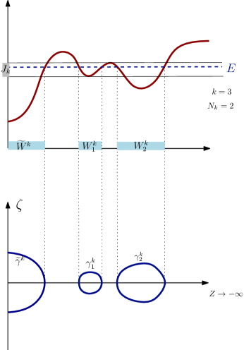
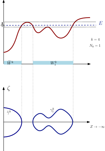
Fig. 1: Wells of different orders and periodic trajectories.

Similar to Proposition 10.1 in [8], we have

Proposition 4.

The semiclassical spectrum mod $o(h^{5/2})$ in $J_{k}$ is the union of $N_{k}+1$ spectra: $\cup_{j=1}^{N_{k}}\Sigma_{j}^{k}(h)\cup\widetilde{\Sigma}^{k}(h)$. Here, $\Sigma_{j}^{k}(h)$ is the semiclassical spectrum associated to well $W_{j}^{k}$, and $\widetilde{\Sigma}^{k}(h)$ is the semiclassical spectrum for half well $\widetilde{W}^{k}$.

The above separation of semiclassical spectra comes from the fact that the eigenfunctions are $\mathcal{O}(h^{\infty})$ outside the wells, and is related to the exponentially small “tunneling” effects [16, 42]. We refer further to [2] for more details. Therefore, we have Bohr-Sommerfeld rules for separated wells, that is,

(36) $$\Sigma_{j}^{k}(h)=\{\mu_{\alpha}(h)\ :\ E_{k-1}<\mu_{\alpha}(h)<E_{k}\text{ and }S^{k,j}(\mu_{\alpha}(h))=2\pi h\alpha\},$$

where $S^{k,j}=S^{k,j}(E):\ ]E_{k-1},E_{k}[\to\mathbb{R}$ admits the asymptotics in $h$

$$S^{k,j}(E)=S^{k,j}_{0}(E)+h\pi+h^{2}S_{2}^{k,j}(E)+\cdots$$

and

(37) $$\widetilde{\Sigma}^{k}(h)=\{\nu_{\alpha}(h)\ :\ E_{k-1}<\nu_{\alpha}(h)<E_{k}\text{ and }\widetilde{S}^{k}(\nu_{\alpha}(h))=2\pi h\alpha\},$$

where $\widetilde{S}^{k}=\widetilde{S}^{k}(E):\ ]E_{k-1},E_{k}[\to\mathbb{R}$ admits the asymptotics

$$\widetilde{S}^{k}(E)=\frac{1}{2}\tilde{S}^{k}_{0}(E)+\frac{3}{2}h\pi+\frac{1}{2}h^{2}\widetilde{S}_{2}^{k}(E)+\cdots.$$

The form of $S^{k,j}$ is similar to the one given in (34)-(33) and the form of $\widetilde{S}^{k}$ is similar to the one given in (28)-(31). We will give more details below.

For alternative representations of $S^{k,j}$ and $\widetilde{S}^{k}$, we introduce the classical Hamiltonian $p_{0}(Z,\zeta)=\hat{\mu}(Z)(1+\zeta^{2})$. For any $k$, $p_{0}^{-1}(J_{k})$ is a union of $N_{k}$ topological annuli $A_{j}^{k}$ and a half annulus $\widetilde{A}^{k}$. The map $p_{0}:\ A_{j}^{k}\to J_{k}$ is a fibration whose fibers $p_{0}^{-1}(E)\cap A_{j}^{k}$ are topological circles $\gamma_{j}^{k}(E)$ that are periodic trajectories of classical dynamics (illustrated in Figure 1 bottom). The map $p_{0}:\ \widetilde{A}^{k}\to J_{k}$ is a topological half circle $\widetilde{\gamma}^{k}(E)$. If $E\in J_{k}$ then $p_{0}^{-1}(E)=(\cup_{j=1}^{N_{k}}\gamma_{j}^{k}(E))\cup\widetilde{\gamma}^{k}(E)$. The corresponding classical periods are

$$T_{j}^{k}(E)=\int_{\gamma_{j}^{k}(E)}|\mathrm{d}t|.$$

We let $t$ be the parametrization of $\gamma^{k}_{j}(E)$ by time evolution in

(38) $$\frac{\mathrm{d}Z}{\mathrm{d}t}=\partial_{\zeta}p_{0},\quad\frac{\mathrm{d}\zeta}{\mathrm{d}t}=-\partial_{Z}p_{0}$$

for a realized energy level $E$.

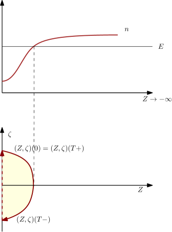
Fig. 2: Behavior of a half trajectory.

For the half well $\widetilde{W}_{k}$, $(Z,\zeta)$ follows a periodic (half) trajectory as shown in Figure 2. After one (half-) period $T$, the trajectory reaches the boundary $Z(T)=0$, and encounters a perfect reflection, so that

$$\zeta(T+)=-\zeta(T-)=\sqrt{\frac{E-\hat{\mu}(0)}{\hat{\mu}(0)}},$$

and then continues following the Hamilton system (38).

4.3.1 Wells separated from the boundary

For a well $W^{k}_{j}$ separated from the boundary, the associated semiclassical spectrum mod $o(h^{5/2})$ follows from (36) and (32)-(35). We have

(39) $$S^{k,j}(E)=S_{0}^{k,j}(E)+h\pi+h^{2}S_{2}^{k,j}(E),$$

where

(40) $$S_{0}^{k,j}(E)=\int_{\gamma_{j}^{k}(E)}\zeta\mathrm{d}Z={\rm Area}\{(Z,\zeta)\ :\ p_{0}(Z,\zeta)\leq E,\,Z\in W^{k}_{j}\}$$

and

(41) $$S_{2}^{k,j}(E)=-\frac{1}{12}\frac{\mathrm{d}}{\mathrm{d}E}\int_{\gamma^{k}_{j}(E)}\left(E\hat{\mu}^{\prime\prime}-2\frac{(E-\hat{\mu})}{\hat{\mu}}(\hat{\mu}^{\prime})^{2}\right)|\mathrm{d}t|-\frac{1}{4}\int_{\gamma^{k}_{j}(E)}\hat{\mu}^{\prime\prime}|\mathrm{d}t|.$$

The explicit forms of $S_{0}^{k,j}$ and $S_{2}^{k,j}$ are equivalent to those given in (34)-(33). Here, the integration over $]f_{-}(E),f_{+}(E)[$, $E\in[E_{k-1},E_{k}]$, in the $Z$ coordinate has been changed into integration along the periodic trajectory $\gamma$. One can get the same results by using the method in [5, 8]. From (40) it is immediate that

(42) $$(S^{k,j}_{0})^{\prime}(E)=T^{k}_{j}(E).$$

4.3.2 Half well connected to the boundary

For the half well $\widetilde{W}^{k}$ connected to the boundary, we have, mod $\mathcal{O}(h^{2})$,

(43) $$\widetilde{S}^{k}(E)=\frac{1}{2}\widetilde{S}^{k}_{0}(E)+h\frac{3}{2}\pi,$$

where

(44) $$\widetilde{S}^{k}_{0}(E)=2\int_{\widetilde{\gamma}^{k}(E)}\zeta\mathrm{d}Z.$$

The explicit form of $\widetilde{S}^{k}_{0}$ is equivalent to the one given in (28). Here, the integration over $]f(E),0[$, $E\in[E_{k-1},E_{k}]$, in the $Z$ coordinate has been changed into integration along the (half) periodic trajectory $\tilde{\gamma}$. As before, it follows that

(45) $$\frac{1}{2}(\widetilde{S}^{k}_{0})^{\prime}(E)=\frac{1}{2}\widetilde{T}^{k}(E).$$

The explicit form of $\widetilde{S}_{2}^{k}$ will not be needed in the following and hence we omit it.

We note that $S_{0}^{k,j}$ and $\widetilde{S}^{k}_{0}$ depend only on periodic trajectories.

Remark 4.2.

In the further analysis of the inverse problem, the explicit form of $S_{2}^{k}$ is only needed for the wells separated from the boundary (between two turning points) and there the formulas are exactly as in [8] (on the whole line without boundary conditions). Near the boundary (between a turning point and the boundary) the function $\hat{\mu}$ is strictly decreasing and only $S_{0}^{k}$ or the counting function for semiclassical eigenvalues suffice to reconstruct the profile.

5 Unique recovery of $\hat{\mu}$ from the semiclassical spectrum

5.1 Trace formula

The inverse problem is addressed with a trace formula as it reflects the data.

Lemma 5 ([8], Lemma 11.1).

Let $S:\ J\to{\mathbb{R}}$ be a smooth function with $S^{\prime}>0$. Then we have the following identity as Schwartz distributions in $J$, meaning that the equality holds when applying both sides to a test function $\phi\in C_{0}^{\infty}(J)$,

(46) $$\sum_{\alpha\in{\mathbb{Z}}}\delta(E-S^{-1}(2\pi h\alpha))=\frac{1}{2\pi h}\sum_{m\in{\mathbb{Z}}}e^{\mathrm{i}mS(E)/h}S^{\prime}(E).$$

Substituting the action in (39), (43) and the Bohr-Sommerfeld rules in (46) yields, on $J_{k}$ with $\{\mu_{\alpha}(h)\}_{\alpha}=\cup_{j=1}^{N_{k}}\Sigma_{j}^{k}(h)$,

$$\sum_{\alpha\in{\mathbb{Z}}}\delta(E-\mu_{\alpha}(h))= \frac{1}{2\pi h}\sum_{j=1}^{N_{k}}\sum_{m\in{\mathbb{Z}}}e^{\mathrm{i}m(S_{0}^{k,j}(E)h^{-1}+\pi+hS_{2}^{k,j}(E)+{\mathcal{O}}(h^{2}))}(({S^{k,j}_{0}})^{\prime}(E)+h^{2}({S^{k,j}_{2}})^{\prime}(E)+{\mathcal{O}}(h^{3}))$$

$$= \frac{1}{2\pi h}\sum_{j=1}^{N_{k}}\sum_{m\in{\mathbb{Z}}}e^{\mathrm{i}mS_{0}^{k,j}(E)h^{-1}}e^{\mathrm{i}m\pi}({S^{k,j}_{0}})^{\prime}(E)(1+\mathrm{i}mhS_{2}^{k,j}(E)+{\mathcal{O}}(h^{2}))$$

and with $\{\nu_{\alpha}(h)\}_{\alpha}\subset\widetilde{\Sigma}^{k}(h)$,

$$\sum_{\alpha\in{\mathbb{Z}}}\delta(E-\nu_{\alpha}(h))= \frac{1}{2\pi h}\sum_{m\in{\mathbb{Z}}}e^{\mathrm{i}m(\frac{1}{2}\widetilde{S}_{0}^{k}(E)h^{-1}+\frac{3}{2}\pi+h\frac{1}{2}\widetilde{S}_{2}^{k}(E)+{\mathcal{O}}(h^{2}))}\left(\frac{1}{2}(\widetilde{S}^{k}_{0})^{\prime}(E)+\frac{h^{2}}{2}(\widetilde{S}^{k}_{2})^{\prime}(E)+{\mathcal{O}}(h^{3})\right)$$

$$= \frac{1}{2\pi h}\sum_{m\in{\mathbb{Z}}}e^{\mathrm{i}m\frac{1}{2}\widetilde{S}_{0}^{k}(E)h^{-1}}e^{\mathrm{i}m\frac{3}{2}\pi}\frac{1}{2}(\widetilde{S}^{k}_{0})^{\prime}(E)\left(1+\mathrm{i}mh\frac{1}{2}\widetilde{S}_{2}^{k}(E)+{\mathcal{O}}(h^{2})\right).$$

Using (42) and (45), and writing $\mu_{\alpha}$ for $\nu_{\alpha}$ in a unified notation, we obtain the trace formula in

Theorem 6.

Let $\mu_{\alpha}(h)$ be the semiclassical spectrum modulo $o(h^{5/2})$. As distributions on $J_{k}$, we have

$$\sum_{\alpha\in{\mathbb{Z}}}\delta(E-\mu_{\alpha}(h))= \frac{1}{2\pi h}\sum_{j=1}^{N_{k}}\sum_{m\in{\mathbb{Z}}}(-1)^{m}e^{\mathrm{i}mS_{0}^{k,j}(E)h^{-1}}T^{k}_{j}(E)(1+\mathrm{i}mhS_{2}^{k,j}(E))$$

(47) $$+\frac{1}{2\pi h}\sum_{m\in{\mathbb{Z}}}e^{\mathrm{i}m\frac{1}{2}\widetilde{S}_{0}^{k}(E)h^{-1}}e^{\mathrm{i}m\frac{3}{2}\pi}\widetilde{T}^{k}(E)\left(1+\mathrm{i}mh\frac{1}{2}\widetilde{S}^{k}_{2}(E)\right)+o(1).$$

The direct way to obtain this trace formula is starting from (2.1), that is,

$$\int_{\mathbb{R}^{-}}\widehat{\epsilon\partial_{t}\mathcal{G}_{0}}(Z,x,\omega,Z,\xi;\epsilon)\mathrm{d}(\epsilon Z)\sim\frac{1}{2h^{2}}\sum_{\alpha\in{\mathbb{Z}}}\delta(E-\mu_{\alpha}(h)),$$

upon substituting $E=h^{2}\omega^{2}$. We then expand the parametrix $(\ref{G0})$ in the WKB eigenfunctions $(\ref{WKB})$ from the previous section.

We will use the notation

(48) $$Z^{k}_{m,j}(E) = \frac{1}{2\pi h}(-1)^{m}e^{\mathrm{i}mS^{k,j}_{0}(E)h^{-1}}T^{k}_{j}(E)(1+\mathrm{i}mhS^{k,j}_{2}(E)),\quad j=1,\cdots,N_{k},$$

(49) $$Z^{k}_{m,N_{k}+1}(E) = \frac{1}{2\pi h}e^{\mathrm{i}m\frac{3}{2}\pi}e^{\mathrm{i}m\frac{1}{2}\widetilde{S}^{k}_{0}(E)h^{-1}}T^{k}_{N_{k}+1}(E)\left(1+\mathrm{i}mh\frac{1}{2}\widetilde{S}^{k}_{2}(E)\right),$$

(50) $$T^{k}_{N_{k}+1}(E): = \widetilde{T}^{k}(E)$$

for $m\in{\mathbb{Z}}$. To further unify the notation, we write

$$S^{k,N_{k}+1}_{0,2}(E):=\frac{1}{2}\widetilde{S}^{k}_{0,2}(E).$$

The micro-support of $Z^{k}_{m,j}$, $j=1,\cdots,N_{k}+1$, is given by the Lagrangian submanifold

$$L^{k}_{m,j}=\{(E,mT^{k}_{j}(E))\ :\ E\in J_{k}\}$$

of $T^{*}J_{k}$ associated with phase function $mS^{k,j}_{0}(E)$.

5.2 Separation of clusters and the weak transversality condition

We observe that the singular points of the counting function, $\int_{p_{0}(Z,\zeta)\leq E}|\mathrm{d}Z\mathrm{d}\zeta|$, are precisely the critical values, $E_{1},E_{2},\cdots,E_{M}$, of $\hat{\mu}$ [8, Lemma 11.1] and, hence, are determined using the Weyl asymptotics first. From the singularity at $E_{k}$ one can extract the value of $\hat{\mu}^{\prime\prime}(Z_{k})$. We then invoke

Assumption 5.1.

For any $k=1,2,\cdots$ and any $j$ with $1\leq j<l\leq N_{k}+1$, the classical periods (half-period if $j=N_{k}+1$) $T^{k}_{j}(E)$ and $T^{k}_{l}(E)$ are weakly transverse in $J_{k}$, that is, there exists an integer $N$ such that the $N$th derivative $(T^{k}_{j}-T^{k}_{l})^{(N)}(E)$ does not vanish.

We introduce the sets

$$B=\{E\in J_{k}\ :\ \exists j\neq l,\quad T^{k}_{j}(E)=T^{k}_{l}(E)\},$$

while suppressing $k$ in the notation. By the weak transversality assumption, it follows that $B$ is a discrete subset of $J_{k}$.

We let the distributions $D_{h}(E)=\sum_{\alpha\in{\mathbb{Z}}}\delta(E-\mu_{\alpha}(h))$ be given on intervals $J=J_{k}$ modulo $o(1)$ using (47). These distributions are determined mod $o(1)$ by the semiclassical spectra mod $o(h^{5/2})$. We denote by $Z_{h}$ the finite sum defined by the right-hand side of (47) restricted to $m=1$, that is,

$$Z_{h}(E)=\sum_{j=1}^{N_{k}+1}Z^{k}_{1,j}(E).$$

By analyzing the micro-support of $D_{h}$ and $Z_{h}$ [8, Lemmas 12.2 and 12.3], we find

Lemma 7.

Under the weak transversality assumption, the sets $B$ and the distributions $Z_{h}$ mod $o(1)$ are determined by the distributions $D_{h}$ mod $o(1)$.

Lemma 8.

Assuming that the $S^{j}$’s are smooth and the $a_{j}$’s do not vanish, there is a unique splitting of $Z_{h}$ as a sum

$$Z_{h}(E)=\frac{1}{2\pi h}\sum_{j=1}^{N_{k}+1}(a_{j}(E)+hb_{j}(E))e^{\mathrm{i}S^{j}(E)/h}+o(1).$$

It follows that the spectrum in $J_{k}$ mod $o(h^{5/2})$ determines the actions $S^{k,j}_{0}(E)$, $S^{k,j}_{2}(E)$ and $\widetilde{S}^{k}_{0}(E)$. This provides the separation of the data for the $N_{k}$ wells and the half well.

For the reconstruction of $\hat{\mu}$ from these actions, we need one more assumption

Assumption 5.2.

The function $\hat{\mu}$ has a generic symmetry defect: If there exist $X_{\pm}$ satisfying $\hat{\mu}(X_{-})=\hat{\mu}(X_{+})<E$, and for all $N\in{\mathbb{N}}$, $\hat{\mu}^{(N)}(X_{-})=(-1)^{N}\hat{\mu}^{(N)}(X_{+})$, then $\hat{\mu}$ is globally even with respect to ${\frac{1}{2}}(X_{+}+X_{-})$ in the interval $\{Z\ :\ \hat{\mu}(Z)<E\}$.

We will carry out the reconstruction of $\hat{\mu}$ successively in intervals $J_{k}$, $k=1,\cdots,M$ and then on the interval $[E_{M},E_{M+1}]$ with $E_{M+1}=\hat{\mu}_{I}$.

5.3 Reconstruction of a single well, with barrier and descreasing profile

We discuss in detail the case of one local minimum for $Z<0$ and global minimum at $Z=0$ ($\hat{\mu}(0)<\hat{\mu}(Z)$ $\forall$ $Z<0$, $\hat{\mu}^{\prime}(0)\leq 0$). This means that the global minimum occurs at $Z=0$ and $E_{1}=\hat{\mu}(Z_{1})$ is the local minimum. Then $E_{2}=\hat{\mu}(Z_{2})$ is attained at $Z_{2}\in(Z_{1},0)$ and $E_{3}=\hat{\mu}_{I}$.

Step 1. For $E\in]E_{0},E_{1}[$, there is only one (half) well, $\widetilde{W}^{1}(E)$, of order $1$ with $\widetilde{W}^{1}(E_{1})=[Z_{1}^{\prime},0]$. Since $\hat{\mu}$ is strictly decreasing in $\widetilde{W}^{1}(E_{1})$, we may reconstruct $\hat{\mu}$ on this interval as in Section 3. This is illustrated in Figure 3 in green.

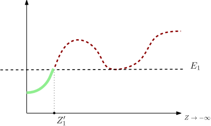
Fig. 3: Reconstruction Step 1 in green.

Step 2. We note that $Z_{2}$ in this case is the $Z^{*}$ defined above Assumption 4.1. We consider $E\in\,]E_{1},E_{2}[$ which corresponds to wells of order $k=2$ with $N_{k}=1$ (one connected component for $Z<0$ separated from the boundary). The two wells are $W^{2,1}(E)$ and $\widetilde{W}^{2}(E)$ with $W^{2,1}(E_{2})=[Z_{-},Z_{2}]$ and $\widetilde{W}^{2}(E_{2})=[Z_{2},0]$. Here, $Z_{-}$ is the unique point in $[Z_{I},Z_{1}]$ such that $E_{2}=\hat{\mu}(Z_{-})$. We are given $S^{2,1}_{0}$, $S^{2,1}_{2}$ and $\widetilde{S}^{2}_{0}$ (and $\widetilde{S}^{2}_{2}$).

We continue to reconstruct $\hat{\mu}$ from $[Z^{\prime}_{1},0]$ to $[Z_{2},0]$ from $\widetilde{S}_{0}^{2}$. For the reconstruction of $\hat{\mu}$ on the interval $I=[Z_{-},Z_{2}]$, more effort is needed. We note that, up to this point, $I$ itself cannot be determined yet. The following theorem is a version of [8, Theorem 5.1]

Theorem 9.

Under Assumption 5.2, the function $\hat{\mu}$ is determined on $I$ by $S_{0}^{2,1}$ and $S_{2}^{2,1}$ up to a symmetry $\hat{\mu}(Z)\rightarrow\hat{\mu}(c-Z)$, where $\frac{c}{2}$ is the midpoint of $I$.

Proof.

For any $E\in[E_{1},E_{2}[$ the functions $f_{\pm}:\ [E_{1},E_{2}[\to I$, are defined so that $W^{2}_{1}(E)=[f_{-}(E),f_{+}(E)]$. We have $\hat{\mu}^{\prime}(Z)<0$ for $Z\in\,]f_{-}(E),Z_{1}[$ and $\hat{\mu}^{\prime}(Z)>0$ for $Z\in\,]Z_{1},f_{+}(E)[$. We introduce

$$\Phi(E)=f_{+}^{\prime}(E)-f_{-}^{\prime}(E)\quad\text{and}\quad\Psi(E)=\frac{1}{f_{+}^{\prime}(E)}-\frac{1}{f_{-}^{\prime}(E)}.$$

As in the proof of Theorem 3, we have

$$(S^{2,1}_{0})^{\prime}(E)=Tg(E),\quad Tg(E)=\int_{E_{1}}^{E}\frac{g(u)}{\sqrt{E-u}}\,\mathrm{d}u\quad\text{with}\quad g(u)=\frac{\Phi(u)}{\sqrt{u}}.$$

The inversion formula for the Abel transform yields $\Phi(E)$ for $E\in[E_{1},E_{2}[$.

Concerning the recovery of $\Psi$, we have

$$S^{2,1}_{2}(E)=-\frac{1}{12}\frac{\mathrm{d}}{\mathrm{d}E}\mathcal{B}\Psi(E),\quad\mathcal{B}\Psi(E)=\int_{E_{1}}^{E}\left((7E-6u)\Psi^{\prime}(u)-2\left(\frac{E}{u}-1\right)\Psi(u)\right)\frac{\mathrm{d}u}{\sqrt{u(E-u)}},$$

which follows from (35) with (32)-(33) upon changing variable of integration, $Z=f_{\pm}(u)$. Thus, from $S^{2,1}_{2}(E)$ and the fact $\mathcal{B}\Psi(E_{1})=\pi\sqrt{2E_{1}\hat{\mu}^{\prime\prime}(Z_{1})}$, we can recover $\mathcal{B}\Psi(E)$. It can be shown that

$$\frac{\pi}{E^{3/2}}\frac{\mathrm{d}^{2}}{\mathrm{d}E^{2}}(T\circ\mathcal{B}\Psi)(E)=E^{2}\Psi^{\prime\prime}(E)+4E\Psi^{\prime}(E)-\Psi(E).$$

That is, we obtain a second-order inhomogeneous ordinary differential equation for $\Psi$ on the interval $[E_{1},E_{2}[$. This equation is supplemented with the “initial” conditions

$$\Psi(E_{1})=0,\quad\lim_{E\downarrow E_{1}}\sqrt{E-E_{1}}\Psi^{\prime}(E)=\sqrt{2\hat{\mu}^{\prime\prime}(Z_{1})}$$

As mentioned in Subsection 5.2, this second derivative is obtained from the limiting behavior of the counting function which coincides with $S^{2,1}_{0}(E)$ as $E\downarrow E_{1}$. We use that the period of small oscillations of the “pendulum” associated to the local minimum of $\hat{\mu}$ at $Z_{1}$ is given by

$$(S^{2,1}_{0})^{\prime}(E)=\int_{f_{-}(E)}^{f_{+}(E)}\frac{\mathrm{d}Z}{\sqrt{\hat{\mu}(E-\hat{\mu})}}=\pi\sqrt{\frac{2}{E_{1}\hat{\mu}^{\prime\prime}(Z_{1})}}+o(1)\quad\text{as}\ E\downarrow E_{1}.$$

Thus we obtain $\Psi(E)$ for $E\in[E_{1},E_{2}[$.

With $\pm f_{\pm}^{\prime}(E)>0$ for $E\in\,]E_{1},E_{2}[$, we then find

(51) $$2f_{\pm}^{\prime}=\pm\Phi+\sigma\sqrt{\Phi^{2}-4\frac{\Phi}{\Psi}}$$

with

$$\sigma=\mathop{\rm sign}\nolimits(f_{+}^{\prime}+f_{-}^{\prime})=\left\{\begin{array}[]{ccc}+1&\text{if}&f_{+}^{\prime}+f_{-}^{\prime}>0\\ 0&\text{if}&f_{+}^{\prime}+f_{-}^{\prime}=0\\ -1&\text{if}&f_{+}^{\prime}+f_{-}^{\prime}<0\end{array}\right.$$

We note that the sign is not (yet) determined, and only if the well is mirror-symmetric with respect to its vertex then $f_{+}^{\prime}+f_{-}^{\prime}=0$ and the square root in (51) vanishes. However, later, we will find the sign by a gluing argument.

By Assumption 5.2, the function $\sigma=\sigma(E)$ is constant for $E\in\,]E_{1},E_{2}[$. Hence, in what follows we will exchange $\sigma$ with $\pm$. We have

$$f_{+}(E) = Z_{1}+\frac{1}{2}\int_{E_{1}}^{E}\left(\Phi\pm\sqrt{\Phi^{2}-4\frac{\Phi}{\Psi}}\right)\mathrm{d}E,$$

$$f_{-}(E) = Z_{1}+\frac{1}{2}\int_{E_{1}}^{E}\left(-\Phi\pm\sqrt{\Phi^{2}-4\frac{\Phi}{\Psi}}\right)\mathrm{d}E.$$

Since $f_{+}(E_{2})=Z_{2}$ and $f_{-}(E_{2})=Z_{-}$, we find that

$$Z_{2} = Z_{1}+\frac{1}{2}\int_{E_{1}}^{E_{2}}\left(\Phi\pm\sqrt{\Phi^{2}-4\frac{\Phi}{\Psi}}\right)\mathrm{d}E,$$

$$Z_{-} = Z_{1}+\frac{1}{2}\int_{E_{1}}^{E_{2}}\left(-\Phi\pm\sqrt{\Phi^{2}-4\frac{\Phi}{\Psi}}\right)\mathrm{d}E.$$

Hence, the distance, $Z_{2}-Z_{1}$, between the two critical points is recovered (modulo mirror symmetry of $Z_{1}$ with respect to $\frac{c}{2}$). Since $f_{\pm}$ are both monotonic on $]E_{1},E_{2}[$, $\hat{\mu}$ can be recovered (up to mirror symmetry) on $I$. ∎

With this result, the reconstructions on $[Z^{\prime}_{1},0]$ and $I$ can be smoothly glued together, and the uncertainty in the translation of $I$ and the “orientation” of $\hat{\mu}$ on $I$ are eliminated. Thus $\hat{\mu}$ is uniquely determined on the interval $[Z_{-},0]$. This is illustrated in Figure 4.

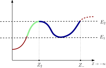
Fig. 4: Reconstruction Step 2, first part in green and second part in blue.

Step 3. On the interval $[Z_{I},Z_{-}]$ we may use the Weyl asymptotics again to recover $\hat{\mu}$. The counting function in the interval $[E_{2},E_{3}]$ is obtained from $\widetilde{S}^{3}$ which corresponds with

$${\rm Area}(\{(Z,\zeta)\ :\ \hat{\mu}(Z)(1+\zeta^{2})\leq E\})=A_{1}(E)+A_{2}(E),$$

where

$$A_{1}(E)={\rm Area}(\{(Z,\zeta)\ :\ \hat{\mu}(Z)(1+\zeta^{2})\leq E,\ Z_{-}\leq Z\leq 0\})$$

is already known, and

$$A_{2}(E)=2\int_{f(E)}^{Z_{-}}\sqrt{\frac{E-\hat{\mu}}{\hat{\mu}}}\mathrm{d}Z,$$

$Z_{I}\leq f(E)<Z_{-}$ since $E_{2}\leq E\leq E_{3}=\hat{\mu}_{I}$. Thus we may recover $\hat{\mu}$ on the interval $[Z_{I},Z_{-}]$ where $\hat{\mu}$ is decreasing while applying Theorem 3. Step 3 is illustrated in Figure 5.

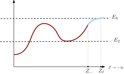
Fig. 5: Reconstruction Step 3 in light blue.

The two profiles for $\hat{\mu}$ on $[Z_{I},Z_{-}]$ and on $[Z_{-},Z_{2}]$ are then glued together at $Z=Z_{-}$ which is already known. This completes the reconstruction procedure.

5.4 Reconstruction of multiple wells

If $\hat{\mu}$ has multiple wells, we follow an inductive procedure. First, we consider the reconstruction of the half well $\widetilde{W}^{k}$ of order $k$ between $E_{k-1}$ and $E_{k}$. We note that $\widetilde{W}^{k}$ must be a continuation of the half well $\widetilde{W}^{k-1}$, or be joined with some well $W^{k-1}_{j^{\prime}}$ of order $k-1$. This can be done in a fashion similar to the process presented above (on $[Z_{I},Z_{-}]$).

Secondly, we consider the reconstruction of a well, $W^{k}_{j}$, separated from the boundary, of order $k$. The well $W^{k}_{j}$ might be a new well, and can be reconstructed as in Theorem 9. The well, $W^{k}_{j}$, might also be joining two wells of order $k-1$, or extending a single well of order $k-1$. Let the profile under $E_{k-1}$ already be recovered. The smooth joining of two wells can be carried out under Assumption 5.2. We consider now functions $f_{-}(E)$ and $f_{+}(E)$ for $E\in[E_{k-1},E_{k}]$ such that $W^{k}_{j}$ is the union of three connected intervals,

$$W^{k}_{j}(E_{k})=[f_{-}(E_{k}),f_{-}(E_{k-1})[\,\cup\,[f_{-}(E_{k-1}),f_{+}(E_{k-1})]\,\cup\,]f_{+}(E_{k-1}),f_{+}(E_{k})];$$

see Figure 6. The semiclassical spectrum in $]E_{k-1},E_{k}[$ up to $o(h^{5/2})$ gives the actions $S^{k,j}_{0}$ and $S^{k,j}_{2}$.

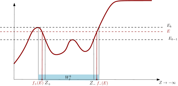
Fig. 6: Illustration of $f_{\pm}$.

From $S^{k,j}_{0}$ we obtain

$$T^{k}_{j}(E)=(S^{k,j}_{0})^{\prime}(E)=\int_{f_{-}(E)}^{f_{+}(E)}\frac{\mathrm{d}Z}{\sqrt{\hat{\mu}(E-\hat{\mu})}}$$

which signify the periods of the trajectories of energy $E$. We write $Z_{-}=f_{-}(E_{k-1})$ and $Z_{+}=f_{+}(E_{k-1})$, and decompose the interval,

$$[f_{-}(E),f_{+}(E)]=[f_{-}(E),Z_{-}]\cup[Z_{-},Z_{+}]\cup[Z_{+},f_{+}(E)].$$

In accordance with this decomposition,

$$T^{k}_{j}(E)=T_{-}(E)+T_{k-1}(E)+T_{+}(E),$$

where

$$T_{-}(E) = \int_{f_{-}(E)}^{Z_{-}}\frac{\mathrm{d}Z}{\sqrt{\hat{\mu}(E-\hat{\mu})}},$$

$$T_{k-1}(E) = \int_{Z_{-}}^{Z_{+}}\frac{\mathrm{d}Z}{\sqrt{\hat{\mu}(E-\hat{\mu})}},$$

$$T_{+}(E) = \int_{Z_{+}}^{f_{+}(E)}\frac{\mathrm{d}Z}{\sqrt{\hat{\mu}(E-\hat{\mu})}}.$$

We note that $T_{k-1}(E)$ is already known. In $T_{\mp}(E)$ we change the variable of integration, $Z=f_{\mp}(u)$. Using that $\hat{\mu}(f_{\mp}(u))=u$, we get

$$T_{\mp}(E)=\mp\int_{E_{k-1}}^{E}\frac{f_{\mp}^{\prime}(u)}{\sqrt{u(E-u)}}\mathrm{d}u;$$

then

$$T^{k}_{j}(E)-T_{k-1}(E)=Tg(E),\quad Tg(E)=\int_{E_{k-1}}^{E}\frac{g(u)}{\sqrt{E-u}}\mathrm{d}u\quad\text{with}\quad g(u)=\frac{\Phi(u)}{\sqrt{u}}$$

and $\Phi(u)=f_{+}^{\prime}(u)-f_{-}^{\prime}(u)$ as before. Inverting this Abel transform, we obtain $\Phi$ on $[E_{k-1},E_{k}[$.

From $S^{k,j}_{2}$ we obtain

$$-\frac{1}{12}\frac{\mathrm{d}}{\mathrm{d}E}J(E)-\frac{1}{4}K(E),$$

where

$$J(E) = \int_{f_{-}(E)}^{f_{+}(E)}\left(E\hat{\mu}^{\prime\prime}-2\frac{(E-\hat{\mu})}{\hat{\mu}}(\hat{\mu}^{\prime})^{2}\right)\frac{\mathrm{d}Z}{\sqrt{\hat{\mu}(E-\hat{\mu})}},$$

$$K(E) = \int_{f_{-}(E)}^{f_{+}(E)}\hat{\mu}^{\prime\prime}\frac{\mathrm{d}Z}{\sqrt{\hat{\mu}(E-\hat{\mu})}}.$$

Using that

$$\hat{\mu}(f_{\pm}(E))=E,\quad\hat{\mu}^{\prime}|_{Z=f_{\pm}(E)}=\frac{1}{f_{\pm}^{\prime}(E)},\quad\hat{\mu}^{\prime\prime}|_{Z=f_{\pm}(E)}=\left(\frac{1}{f_{\pm}^{\prime}}\right)^{\prime}(E)\frac{1}{f_{\pm}^{\prime}(E)},$$

changing variables of integration in $J$ and $K$, $Z=f_{\pm}(u)$ and introducing

$$\Psi(E)=\frac{1}{f_{+}^{\prime}(E)}-\frac{1}{f_{-}^{\prime}(E)},$$

we have

$$J(E)-J_{k-1}(E) = \int_{E_{k-1}}^{E}\left(E\Psi^{\prime}(u)-2\left(\frac{E}{u}-1\right)\Psi(u)\right)\frac{\mathrm{d}u}{\sqrt{u(E-u)}},$$

$$K(E)-K_{k-1}(E) = \int_{E_{k-1}}^{E}\Psi^{\prime}(u)\frac{\mathrm{d}u}{\sqrt{u(E-u)}},$$

where

$$J_{k-1}(E) = \int_{Z_{-}}^{Z_{+}}\left(E\hat{\mu}^{\prime\prime}-2\frac{(E-\hat{\mu})}{\hat{\mu}}(\hat{\mu}^{\prime})^{2}\right)\frac{\mathrm{d}Z}{\sqrt{\hat{\mu}(E-\hat{\mu})}},$$

$$K_{k-1}(E) = \int_{Z_{-}}^{Z_{+}}\hat{\mu}^{\prime\prime}\frac{\mathrm{d}Z}{\sqrt{\hat{\mu}(E-\hat{\mu})}}$$

are already known. Thus, from $S^{k,j}_{2}$, we recover

$$\mathcal{B}\Psi(E)=\int_{E_{k-1}}^{E}\left((7E-6u)\Psi^{\prime}(u)-2\left(\frac{E}{u}-1\right)\Psi(u)\right)\frac{\mathrm{d}u}{\sqrt{u(E-u)}}.$$

Then similar to the proof of Theorem 9, we recover $\Psi$ on $[E_{k-1},E_{k}[$ by inverting $\mathcal{B}$ through the introduction of a second-order ordinary differential equation.

From $\Phi$ and $\Psi$ we obtain

$$2f_{+}^{\prime}=\Phi\pm\sqrt{\Phi^{2}-4\frac{\Phi}{\Psi}},\quad 2f_{-}^{\prime}=-\Phi\pm\sqrt{\Phi^{2}-4\frac{\Phi}{\Psi}}$$

and then

$$f_{+}(E) = Z_{+}+\frac{1}{2}\int_{E_{k-1}}^{E}\left(\Phi\pm\sqrt{\Phi^{2}-4\frac{\Phi}{\Psi}}\right)\mathrm{d}E,$$

$$f_{-}(E) = Z_{-}+\frac{1}{2}\int_{E_{k-1}}^{E}\left(\Phi\pm\sqrt{\Phi^{2}-4\frac{\Phi}{\Psi}}\right)\mathrm{d}E.$$

From $f_{-}$ we recover $\hat{\mu}$ on the interval $[f_{-}(E),Z_{-}]$ and from $f_{+}$ we recover $\hat{\mu}$ on the interval $[Z_{+},f_{+}(E)]$. The $\pm$ signs in $f_{\pm}$ are disentangled by smoothly joining the newly reconstructed pieces to the previously reconstructed part and Assumption 5.2, as in previous section. Since the profile in $[Z_{-},Z_{+}]$ can only be determined up to translation and symmetry, the determination of the profile in $W^{k}_{j}$ is up to the same translation and symmetry.

The symmetry and translation freedom for all the wells will be gradually eliminated during the whole process. At the final step, there is a single half well connected to the boundary, and then we can reconstruct exactly the entire profile.

References

- [1] V. Babich, B. Chikhachev and T. Yanovskaya, Surface waves in a vertically inhomogeneous elastic half space with weak horizontal inhomogeneity. Izv. Bull. Akad. Sci. USSR, Phys. Solid Earth 4 (1976) pp.24-31.
- [2] C. Bender and S. Orszag, Advanced mathematical methods for scientists and engineers I: Asymptotic methods and perturbation theory, Springer Science & Business Media (2013).
- [3] L. Boschi and G. Ekström, New images of the Earth’s upper mantle from measurements of surface wave phase velocity anomalies, J. Geophys. Res.: Solid Earth 107 (2002) ESE-1.
- [4] J. Brune and J. Dorman, Seismic waves and earth structure in the Canadian Shield, Bull. Seism. Soc. Am. 53 (1963) pp.167-209.
- [5] Y. Colin de Verdière. Bohr-Sommerfeld Rules to All Orders, Ann. Henri Poincaré 6 (2005) pp. 925-936.
- [6] Y. Colin de Verdière, Mathematical Models for passive imaging II: Effective Hamiltonians associated to surface waves, arXiv:math-ph/0610044.
- [7] Y. Colin de Verdière, Semiclassical analysis and passive imaging, Nonlinearity 22 (2009) pp.R45-R75.
- [8] Y. Colin de Verdière. A semi-classical inverse problem II: Reconstruction of the potential. In Geometric aspects of analysis and mechanics 292 (2011) pp.97-119.
- [9] F. Dahlen and J. Tromp, Theoretical Global Seismology, Princeton University Press (1998).
- [10] M.V. de Hoop, A. Iantchenko, G. Nakamura and J. Zhai, Semiclassical analysis of elastic surface waves, arXiv:1709.06521.
- [11] A. Derode, E. Larose, M. Tanter, J. de Rosny, A. Tourin, M. Campillo and M. Fink, Recovering the Green’s function form field-field correlations in an open scattering medium, J. Acoust. Soc. Am. 113 (2004) pp.2973-2976.
- [12] M. Dimassi and J. Sjöstrand, Spectral asymptotics in the semiclassical limit, London Mathematical Society Lecture Notes Series 268, Cambridge University Press (1991).
- [13] A. Dziewonski, Regional differences in dispersion of mantle Rayleigh waves, Geophys. J. Roy. Soc. 22 (1971) pp.289-325.
- [14] J.B. Gaherty, T.H. Jordan and L.S. Gee, Seismic structure of the upper mantle in a Central Pacific corridor, J. Geophys. Res. 101 (1996) pp.22291-22309.
- [15] N.A. Haskell, The dispersion of surface waves on multilayered media, Bull. Seism. Soc. Am. 43 (1953) pp.17-34.
- [16] B. Helffer and J. Sjöstrand, Multiple wells in the semi-classical limit I, Commun. PDE 9 (1984) pp.1934-1944.
- [17] Y.-C. Huang, H. Yao, B.-S. Huang, R.D. van der Hilst, K.-L. Wen, W.-G. Huang and C.-H. Chen, Phase velocity variation at periods of 0.5-3 seconds in the Taipei Basin of Taiwan from correlation of ambient seismic noise, Bull. Seism. Soc. Am. 100 (2010) pp.2250-2263.
- [18] L. Knopoff, Green’s function for eigenvalue problems and the inversion of dispersion data, Geophys. J. Int. 4, Supplement_1 (1961) pp.161-173.
- [19] S. Lebedev and R.D. van der Hilst, Global upper-mantle tomography with the automated multimode inversion of surface and S-wave forms, Geophys. J. Int. 173 (2008) pp.505-518.
- [20] A.L. Lerner-Lam and T.H. Jordan, Earth structure from fundamental and higher-mode waveform analysis, Geophys. J. Roy. Soc. 75 (1983) pp.759-797.
- [21] F.-C. Lin, M.P. Moschetti and M.H. Ritzwoller, Surface wave tomography of the western United States from ambient seismic noise: Rayleigh and Love wave phase velocity maps, Geophys. J. Int. 173 (2008) pp.281-298.
- [22] J.-P. Montagner and T. Tanimoto, Global upper mantle tomography of seismic velocities and anisotropies. J. Geophys. Res. 96 (1991) pp.20337-20351.
- [23] H.C. Nataf, I. Nakanishi and D.L. Anderson, Measurements of mantle wave velocities and inversion for lateral heterogeneities and anisotropy. 3. Inversion, J. Geophys. Res. 91 (1986) pp.7261-7307.
- [24] G. Nolet, Higher Rayleigh modes in Western Europe, Geophys. Res. Lett. 2 (1975) pp.60-62.
- [25] G. Nolet, Partitioned waveform inversion and 2-dimensional structure under the Network of Autonomously Recording Seismographs. J. Geophys. Res. 95 (1990) pp.8499-8512.
- [26] F. Press, Determination of crustal structure from phase velocity of Rayleigh waves I: Southern California, Bull. Seism. Soc. Am. 67 (1956) pp.1647-1658.
- [27] M.H. Ritzwoller, N.M. Shapiro, A.L. Levshin, and G.M. Leahy, The structure of the crust and upper mantle beneath Antarctica and the surrounding oceans, J. Geophys. Res. 06 (2001) pp. 30645-30670.
- [28] J. Ritsema, H.J. van Heijst and J.H. Woodhouse, Global transition zone tomography, J. Geoph. Res.: Solid Earth 109 (2004) B002610.
- [29] K.G. Sabra, P. Gerstoft, P. Roux and W. Kuperman and M.C. Fehler, Surface wave tomography from microseisms in Southern California, Geophys. Res. Lett. 32 (2005) L14311, doi:10.1029/2005GL023155.
- [30] N. Shapiro and M. Campillo, Emergence of broadband Rayleigh waves from correlations of the ambient seismic noise, Geophys. Res. Lett. 31 (2004) L07614, doi:10.1029/2004GL019491.
- [31] N. Shapiro, M. Campillo and L. Stehly and M. Ritzwoller, High resolution surface wave tomography from ambient seismic noise, Science 307 (2005) pp.1615-1618.
- [32] F.A. Schwab and L. Knopoff, Surface waves on multilayered anelastic media. Bull. Seism. Soc. Am. 61 (1971) pp.893-912.
- [33] F.J. Simons, R.D. van der Hilst, J.-P. Montagner and A. Zielhuis, Multimode Rayleigh wave inversion for heterogeneity and azimuthal anisotropy of the Australian upper mantle, Geophys. J. Int. 151 (2002) pp.738-754.
- [34] M.N. Toksöz and D.L. Anderson, Phase velocities of long-period surface waves and structures of the upper mantle, I. Great-circle Love and Rayleigh wave data, J. Geophys. Res. 71 (1961) pp.1649-1658.
- [35] J. Trampert and J.H. Woodhouse, Global phase velocity maps of Love and Rayleigh waves between 40 and 150 s period, Geophys. J. Int., 122 (1995) pp.675-690.
- [36] J.H. Woodhouse, Surface waves in a laterally varying layered structure Geophys. J. Roy. Astron. Soc. 37 (1974) pp.461-490.
- [37] J.H. Woodhouse and A.M. Dziewonski, Mapping the upper mantle: Three-dimensional modeling of Earth structure by inversion of seismic waveforms, J. Geophys. Res. 89 (1984) pp.5953-5986.
- [38] Y. Yang, M.H. Ritzwoller, A.L. Levshin and N.M. Shapiro, Ambient noise Rayleigh wave tomography across Europe, Geophys. J. Int. 168 (2007) pp.259-274.
- [39] H. Yao, R.D. van der Hilst and M.V. de Hoop, Surface-wave array tomography in SE Tibet from ambient seismic noise and twostation analysis-I. Phase velocity maps, Geophys. J. Int. 166 (2006) pp.732-744.
- [40] H. Yao, R.D. van der Hilst and J.-P. Montagner, Heterogeneity and anisotropy of the lithosphere of SE Tibet from surface wave array tomography, J. Geophys. Res.: Solid Earth 115 (2010) B12307, doi:10.1029/2009JB007142.
- [41] L. Zhao and F.A. Dahlen, Asymptotic eigenfrequencies of the Earth’s normal modes, Geophys. J. Int 115 (1993) pp.729-758.
- [42] S. Zelditch, The inverse spectral problem, Surveys in Differential Geometry IX (2004) pp.401-467.