Testing the Tremaine-Weinberg Method Applied to Integral-field Spectroscopic Data Using a Simulated Barred Galaxy

Abstract

Tremaine and Weinberg (TW) proposed a conceptually simple procedure relying on long-slit spectroscopy to measure the pattern speeds of bars ($\Omega_{\rm p}$) in disk galaxies. Using a simulated galaxy, we investigate the potential biases and uncertainties of TW measurements using increasingly popular integral-field spectrographs (IFSs), for which multiple pseudo-slits (and thus independent measurements) can be constructed with a single observation. Most importantly, to establish the spatial coverage required and ensure the validity of the measurements, the inferred $\Omega_{\rm p}$ must asymptotically converge as the (half-)length of each pseudo-slit used is increased. The requirement for our simulation is to reach $\approx 1.3$ times the half-light radius, but this may vary from galaxy to galaxy. Only those slits located within the bar region yield accurate measurements. We confirm that the position angle of the disk is the dominant source of systematic error in TW $\Omega_{\rm p}$ measurements, leading to under/overestimates of tens of percent for inaccuracies of even a few degrees. Recasting the data so that the data grid aligns with the disk major axis leads to slightly reduced uncertainties. Accurate measurements are obtained only for well-defined ranges of the bar angle (relative to the galaxy major axis) $\phi_{\rm bar}$ and the inclination angle $i$, here $10\arcdeg\lesssim\phi_{\rm bar}\lesssim 75\arcdeg$ and $105\arcdeg\lesssim\phi_{\rm bar}\lesssim 170\arcdeg$ and $15\arcdeg\lesssim i\lesssim 70\arcdeg$. The adopted (pseudo-)slit widths, spatial resolution, and (unless extremely aggressive) spatial binning of IFS data have no significant impact on the measurements. Our results thus provide useful guidelines for reliable and accurate direct $\Omega_{\rm p}$ measurements with IFS observations.

1 Introduction

Bars are present in at least half of nearby disk galaxies (e.g. Eskridge et al., 2000; Marinova & Jogee, 2007; Menéndez-Delmestre et al., 2007; Barazza et al., 2008; Aguerri et al., 2009). They play an important role in the redistribution of angular momentum and energy across the different components of the host disk, as well as between the disk and dark matter halo (e.g. Weinberg, 1985; Debattista & Sellwood, 1998, 2000; Athanassoula, 2003). The dynamics of barred galaxies depends primarily (but not exclusively) on the angular velocity or pattern speed of the bar, denoted $\Omega_{\rm p}$. Usually, $\Omega_{\rm p}$ is parameterized by the dimensionless bar rotation rate $\mathcal{R}\equiv R_{\rm CR}/a_{\rm bar}$, where $a_{\rm bar}$ is the half-length of the bar and the corotation radius $R_{\rm CR}$ (where the bar rotation speed equals that of disk material) can be determined from the disk circular velocity curve and $\Omega_{\rm p}$. Fast bars are defined as having $1\leq\mathcal{R}\leq 1.4$ while slow bars have $\mathcal{R}>1.4$ (Debattista & Sellwood, 2000); $\mathcal{R}<1$ is not allowed by the orbital structure of barred disks (e.g. Contopoulos, 1980; Athanassoula, 1992a).

The measurement of $\Omega_{\rm p}$ is challenging. There are a variety of methods in the literature to indirectly measure bar pattern speeds, which are all model dependent. In particular, hydrodynamical simulations of individual barred galaxies have been used to infer $\Omega_{\rm p}$, by matching the observed gas morphology and/or gas velocities with those of a simulated galaxy (e.g. Weiner et al., 2001; Rautiainen et al., 2008; Treuthardt et al., 2008; Fragkoudi et al., 2017). There are also some physically motivated methods to measure $\Omega_{\rm p}$, associating particular morphological features with Lindblad resonances. Specifically, these methods associate the position of galaxy rings with certain resonances (e.g. Buta, 1986; Buta et al., 1995; Vega Beltran et al., 1997; Muñoz-Tuñón et al., 2004; Pérez et al., 2012), they examine the offsets and shapes of dust lanes (e.g. van Albada & Sanders, 1982; Athanassoula, 1992b), they analyze the changes of the morphologies and/or phases of spiral arms near $R_{\rm CR}$ (e.g. Canzian, 1993; Canzian & Allen, 1997; Puerari & Dottori, 1997; Aguerri et al., 1998; Buta & Zhang, 2009), they identify color and star formation changes beyond the bar region (e.g. Cepa & Beckman, 1990; Aguerri et al., 2000), and they characterize the gas and/or stellar velocity residuals after subtraction of the (axisymmetric) rotation pattern (e.g. Sempere et al., 1995; Font et al., 2011, 2014; Beckman et al., 2018). Nevertheless, to gauge their accuracies, most of these indirect methods must still be compared with direct measurements.

The only model-independent way to measure $\Omega_{\rm p}$ is the Tremaine-Weinberg (TW) method (Tremaine & Weinberg, 1984), which uses a simple and elegant formalism to infer $\Omega_{\rm p}$ directly from the data. In this paper, we use an $N$-body simulation to understand the limitations, biases, and uncertainties that can affect TW measurements, particularly when carried out using integral-field spectrographs (IFSs), which necessarily have limited fields of view (FOVs) and angular resolutions (point spread functions [PSFs]). We first review in § 2 the TW formalism and its likely limitations, before describing in § 3 the simulation and mock data sets used to quantify those limitations. § 4 presents analyses of a number of specific potential biases and discusses their likely impact on real measurements. § 5 briefly summarizes the main results.

2 Tremaine-Weinberg Method

2.1 Formalism

As mentioned above, the TW method is the only model-independent means to infer $\Omega_{\rm p}$ from observational data. Its original and simplest implementation uses long-slit spectroscopic observations, under the assumptions that the disk is flat and the bar (actually the whole disk) has a single well-defined pattern speed. Another key requirement is that the (surface brightness of the) tracer population obeys the continuity equation. From these assumptions, $\Omega_{\rm p}$ can be derived as

$$\Omega_{\rm p}\sin i \,=\,\frac{\int_{-\infty}^{+\infty}h(Y)\,dY\int_{-\infty}^{+\infty}\,[V_{||}(X,Y)\!\!-\!\!V_{\rm sys}]\,\Sigma(X,Y)\,dX}{\int_{-\infty}^{+\infty}h(Y)\,dY\int_{-\infty}^{+\infty}\,[X\!\!-\!\!X_{\rm c}]\,\Sigma(X,Y)\,dX}{}$$ (1a)

$${}\,=\,\frac{<V_{||}>\!-V_{\rm sys}}{<X>\!-X_{\rm c}}\,\,\,,$$ (1b)

where ($X$,$Y$) are sky plane coordinates with origin at the galaxy center, $V_{||}(X,Y)$ is the mean line-of-sight (LOS) velocity and $\Sigma(X,Y)$ the surface brightness (or surface mass density) of the tracer adopted, $V_{\rm sys}$ is the galaxy systemic velocity, $X_{\rm c}$ is the position of the galaxy minor axis, and $h(Y)$ is an arbitrary weighting function. The $X$-axis and the $Y$-axis must be aligned with the major and the minor axis of the galaxy disk, respectively, and the slits (one for each $Y$) should thus be aligned parallel to but offset from the disk major axis (so that the integrals along $X$ correspond to summations along slits parallel to but offset from the major axis).

Merrifield & Kuijken (1995) refined the TW method, suggesting to simply collapse the long-slit spectra to yield higher signal-to-noise ratio (S/N) measurements. They thus rewrote Equation 1(a) into the equivalent Equation 1(b), where

$$<V_{||}>\,\equiv\,\frac{\int_{-\infty}^{+\infty}\,V_{||}(X,Y)\,\Sigma(X,Y)\,dX}{\int_{-\infty}^{+\infty}\,\Sigma(X,Y)\,dX}$$ (2)

and

$$<X>\,\equiv\,\frac{\int_{-\infty}^{+\infty}\,X\,\Sigma(X,Y)\,dX}{\int_{-\infty}^{+\infty}\,\Sigma(X,Y)\,dX}$$ (3)

are, respectively, the luminosity-weighted mean velocity and the mean position obtained from collapsing one long-slit spectrum along, respectively, its spatial and its dispersion (wavelength) direction. Then, $\Omega_{\rm p}\sin i$ can easily be obtained from the slope of a straight line fit to $<V_{||}>$ versus $<X>$ for multiple slits. In addition to a single higher-S/N measurement for each of the numerator and denominator in Equation 1(b), another advantage of this procedure is that the uncertainties on $V_{\rm sys}$ and $X_{\rm c}$ are unimportant (while they can lead to systematic biases when using Eq. 1(a) directly). We will refer to this method as the MK method.

The TW method infers the bar pattern speed by quantifying the asymmetries introduced by the bar in the galaxy disk. Indeed, for an axisymmetric disk with no bar, $\Sigma(X,Y)$ is an even function of $X$ (i.e., along the slit), while $V_{||}(X,Y)$ and $X$ are odd functions of $X$. Thus, the integrals in the numerator and denominator of Equation 1 both sum to zero, and $\Omega_{\rm p}$ is undefined. The existence of a bar (or a spiral pattern) introduces an oddness into $\Sigma(X,Y)$ and an evenness into $V_{||}(X,Y)$, resulting in nonzero integrals and the desired measurement of $\Omega_{\rm p}$. This is the main power of the TW method but also its greatest weakness, in that the integrals in the numerator and denominator of Equation 1 effectively take the difference of two large numbers, making TW measurements extremely sensitive to imperfections in the data and prone to systematic biases. In particular, asymmetries due to (sub)structures other than the bar can lead to false signals. It is thus essential to ensure that the contributions to the integrals in Equation 1 are indeed due to the bar and not other artifacts.

There are various ways to measure bar pattern speeds using the TW method. According to Equation 1(a), $\Omega_{\rm p}$ can be measured from a single measurement using a single slit or from the average of multiple measurements using multiple slits (e.g. Kent, 1987; Bureau et al., 1999). We will refer to the latter method as the TW averaging method. As suggested by Equation 1(b), another way to measure $\Omega_{\rm p}$ is to measure the slope of $<V_{||}>$ versus $<X>$. However, instead of collapsing the spectra to measure $<V_{||}>$ and $<X>$, as suggested by Merrifield & Kuijken (1995), $<V_{||}>$ and $<X>$ can equally be derived from measurements of $\Sigma(X,Y)$ and $V_{||}$ at each position along the slits, following Equations 2 and 3 (see, e.g., Aguerri et al., 2015). We will refer to this as the TW fitting method. Overall, there are thus at least four variants of the TW method: the original TW method, the TW averaging method, the TW fitting method, and the MK method. The first two are sensitive to uncertainties in $V_{\rm sys}$ and $X_{\rm c}$ while the last two are not.

The most important assumption of the TW method is arguably that the tracer population satisfies the continuity equation. Clearly, the old stellar populations of S0 galaxies are good targets for the TW method, as star formation (SF) and dust extinction are usually unimportant. As a result, S0 galaxies have been frequent targets of TW studies (e.g. Kent, 1987; Merrifield & Kuijken, 1995; Gerssen et al., 1999; Debattista et al., 2002; Aguerri et al., 2003; Corsini et al., 2003; Gerssen et al., 2003; Debattista & Williams, 2004; Corsini et al., 2007). However, the TW method has also been applied to late-type galaxies, despite risks that SF and dust will affect the measurements (e.g., Gerssen et al., 2003; Treuthardt et al., 2007; Aguerri et al., 2015; Guo et al., 2019). The application of the TW method to gas tracers rather than stars is also more recent and requires more caution. In galaxies, gas will normally cycle through multiple phases (molecular, atomic, and ionized), and any given phase may not obey the continuity equation. However, if the interstellar medium (ISM) is dominated by a single phase, the gas in that dominant phase may then approximately satisfy the continuity equation. TW bar pattern speed measurements have been carried out using observations of H I (e.g., Bureau et al., 1999; Banerjee et al., 2013) and H₂ (e.g., Rand & Wallin, 2004; Zimmer et al., 2004). The ionized gas rarely dominates the ISM by mass, and any line flux does not reliably trace its mass. However, using $N$-body/SPH simulations, Hernandez et al. (2005) found that the TW method could be applied to the ionized gas component to get a rough estimate of $\Omega_{\rm p}$, on the condition that the shock regions are avoided and the measurements are confined to the gaseous bar region. H$\alpha$ has indeed been used numerous times to measure bar pattern speeds with the TW method (e.g. Hernandez et al., 2005; Emsellem et al., 2006; Fathi et al., 2007, 2009; Chemin & Hernandez, 2009; Gabbasov et al., 2009). Most of the above measurements, irrespective of the tracer, suggest that bars rotate fast.

2.2 Application to IFS Data

Observations with IFSs, which yield 3D data, are becoming increasingly popular, and sizeable samples of barred galaxies with a wide range of morphologies can now be selected from large, homogeneous, and often publicly available IFS surveys – e.g. the Calar Alto Legacy Integral-field Spectroscopy Area Survey (CALIFA; Sánchez et al., 2012), Sydney-Australian-Astronomical-Observatory Multi-object Integral-field Spectrograph (SAMI; Croom et al., 2012) survey, and Mapping Nearby Galaxies at Apache Point Observatory (MaNGA; Bundy et al., 2015) survey. IFS observations have unique advantages over long-slit observations for TW measurements. In particular, multiple pseudo-slits can be constructed from a single IFS observation. Most importantly, Debattista (2003, hereafter D03) investigated slit misalignments and found that errors in the position angle of the disk (PA_disk; e.g. from intrinsic disk ellipticities) and thus of the slits significantly and systematically affect TW $\Omega_{\rm p}$ measurements. IFSs naturally allow us to choose the orientation of the pseudo-slits after the observations are obtained, thus allowing us to test for systematic uncertainties associated with the choice of PA_disk.

The use of the TW method with IFS data also differs from that with long-slit observations in several ways.

1. Extensive spatial coverage is very important to the TW method, as the integrals in Equation 1(a) formally range from $-\infty$ to $+\infty$ (see, e.g., Debattista & Williams, 2004; Rand & Wallin, 2004; Zimmer et al., 2004; Chemin & Hernandez, 2009; Fathi et al., 2009; Aguerri et al., 2015; Guo et al., 2019). In practice, the integrals only need to reach the (projected) radius where the disk becomes (nearly) axisymmetric, as the integrands will cancel out at larger distances. There is no specific prescription to identify this radius, and it is likely to be different from galaxy to galaxy. Most long slits extend to the disk outskirts, where $\Omega_{\rm p}$ measurements should asymptotically converge before the slits end. However, many IFSs have a small FOV, and the disks observed may not reach axisymmetry within that FOV. Before using the TW method with IFS data, it is thus essential to establish the minimum spatial coverage required for reliable and accurate TW measurements. This is done in § 4.1.

2. Similarly, IFS data allow us to create (i.e., overlay on the observations) an arbitrary number of pseudo-slits, at arbitrary positions (i.e., at arbitrary offsets from the galaxy major axis). However, it is unclear whether all the resulting measurements will be equally reliable, as the photometric and kinematic signatures of bars necessarily decrease with increasing radius. In § 4.2, we will thus explore how the quality of a measurement varies as a function of the slit position.

3. Spatial binning is commonly used with IFSs to increase the S/N of the data within a given spatial region (i.e., a bin made up of several spaxels), especially in the outer parts of galaxies, where convergence of the TW integrals is necessary. The flux and velocity of each bin are thus altered and effectively replaced by their (luminosity-weighted) spatial averages. As these are the quantities that underlie the TW method, the positions and sizes of the bins are likely to impact TW $\Omega_{\rm p}$ measurements. In § 4.3, we will therefore quantify the effects of spatial binning on these measurements.

4. As the position angle of the disk (PA_disk) is generally not aligned with the grid/axes of the IFS data $(X_{\rm grid},Y_{\rm grid})$, the footprints of pseudo-slits are irregular in shape (at least in terms of the integer spaxels contained within them), an effect absent with long-slit observations. This introduces extra asymmetries and can thus artificially contribute to the integrals in Equation 1(a), potentially affecting the resulting $\Omega_{\rm p}$ measurements. A possible way to eliminate this effect is to calculate the weights/contributions of fractional spaxels along the slits. However, a more straightforward and practical solution is often to simply recast the data grid. We must then test to what extent this grid recasting can affect the measurements, and this is done in § 4.4.

2.3 Application to Both IFS and Long-slit Data

There are other issues that may affect TW bar pattern speed measurements using either IFS or long-slit observations.

1. A clear advantage of using IFS over long-slit data is that the slits’ orientation (implicitly the disk position angle PA_disk) can readily be changed during the TW calculations. Although PA_disk does not appear explicitly in Equation 1, and consequently PA_disk uncertainties are not normally propagated through $\Omega_{\rm p}$ uncertainties, PA_disk directly affects $\Omega_{\rm p}$ measurements using both IFS and long-slit spectra. According to D03, we expect errors on PA_disk to be the largest (and systematic) source of error in TW $\Omega_{\rm p}$ measurements, as the measured $\Omega_{\rm p}$ can be under- or overestimated by $\approx 50\%$ for a misalignment angle $\delta$PA_disk of only $\approx 5\arcdeg$. In particular, it might be that some of the so-called ultrafast bars recently reported in the literature (Guo et al., 2019) are due to such misalignments. We therefore carry out tests analogous to those of D03 in § 4.5.1, exploring a larger range of misalignment angles and different disk view angles. We also explore potential empirical disk position angle diagnostics (§ 4.5.2).

2. The orientation of a barred disk with respect to the observer is very important. In particular, the bar angle relative to the galaxy major axis ($\phi_{\rm bar}$) is crucial. Indeed, if the bar is exactly parallel or perpendicular to the disk major axis, the surface brightness distribution and velocity field will remain symmetric with respect to the disk minor axis. The integrands in Equation 1(a) will thus remain odd, again yielding an undefined $\Omega_{\rm p}$. As TW measurements utilize $V_{||}$, nearly face-on ($i\approx 0\arcdeg$) galaxies will also yield unreliable measurements, while bars are difficult to identify in nearly edge-on ($i\approx 90\arcdeg$) systems (the intrinsic thickness of the disks is then also apparent and may affect the results). We will thus identify the optimal ranges of the relative bar angle and inclination in § 4.6, to derive a prescription to exclude a priori galaxies with inappropriate orientations.

3. There is also no specific rule to choose the optimal slit width to use. Generally, a slit width roughly equal to the PSF has been adopted. Guo et al. (2019) tested two different pseudo-slit widths and reported that they both yielded consistent measurements. We will explicitly test the influence of the slit width on TW $\Omega_{\rm p}$ measurements in § 4.7.

4. Lastly, the limited spatial resolution of the data may affect measurements. Indeed, observations do not yield the intrinsic surface brightness $\Sigma(X,Y)$ and mean velocity $V_{||}(X,Y)$ of the chosen tracer, but rather those quantities convolved by the PSF of the observations $W(X,Y)$, such that the observed surface brightness $\Sigma_{\rm o}(X,Y)$ and velocity field $V_{\rm o}(X,Y)$ are given by

$$\Sigma_{\rm o}(X,Y)=\int W(X\!\!-\!\!X^{\prime},Y\!\!-\!\!Y^{\prime})\,\Sigma(X^{\prime},Y^{\prime})\,dX^{\prime}dY^{\prime}$$ (4)

and

$$V_{\rm o}(X,Y)=\frac{\int W(X\!\!-\!\!X^{\prime},Y\!\!-\!\!Y^{\prime})\,\Sigma(X^{\prime},Y^{\prime})\,V_{||}(X^{\prime},Y^{\prime})\,dX^{\prime}dY^{\prime}}{\Sigma_{\rm o}(X,Y)}\,\,\,.$$ (5)

Tremaine & Weinberg (1984) argued that the limited spatial resolution of observations is unimportant if the PSF $W(X,Y)$ is an even function of $X$, which is usually the case. To verify this, however, we will directly test in § 4.8 how the PSF affects TW $\Omega_{\rm p}$ measurements.

3 Simulation and Mock Data

We use a simulated barred galaxy to investigate all the issues mentioned above (§ 2.2 and 2.3). We first generate mock data sets, and then use them to test the likely influence on real TW measurements of a number of key observational and analysis parameters (FOV, pseudo-slit selection, spatial binning, grid recasting, errors in disk position angle, relative bar angle and inclination, slit width, and PSF).

3.1 Simulation

The $N$-body simulation we adopt is shown in Figure 1. It is a simple simulation of a disk galaxy with $10^{6}$ live particles of total mass $M_{\rm d}=4.25\times 10^{10}$ $M_{\odot}$, evolving in a rigid dark matter halo spherical potential $\Phi(r)=\frac{1}{2}V_{\rm c}^{2}\ln(1+r^{2}/r_{\rm c}^{2})$, where $r$ is the spherical radius, $V_{\rm c}\approx 250$ km s^-1 is the asymptotic circular velocity at infinity, and $r_{\rm c}=15$ kpc is the core radius. The particles are initially distributed in a dynamically cold (Toomre’s $Q\approx 1.5$) axisymmetric exponential disk with a scale length of $\approx 1.9$ kpc and a scale height $\approx 0.2$ kpc. A bar forms spontaneously and quickly buckles in the vertical direction. To create our mock data sets, we selected a snapshot at $2.4$ Gyr (shown in Fig. 1), when the bar is quasi-steady.

We measure a maximum bar ellipticity $\epsilon_{\rm bar,max}\approx 0.47$ using the Image Reduction and Analysis Facility (IRAF; Tody, 1986, 1993) Ellipse task, from the first maximum of the radial profile of ellipticity of the isophotes. We estimate the bar (half-)length to be $a_{\rm bar}\approx 4.6$ kpc, from the average of the radius of the first minimum in the radial ellipticity profile (4.7 kpc) and the radius suggested by the bar-interbar contrast method (4.5 kpc; see Aguerri et al. 2000). This maximum ellipticity and the (half-)length of the bar compare favorably to those of typical bars (see, e.g., Marinova & Jogee, 2007), although we could of course rescale our simulation to any desired physical size. The simulated galaxy effective (half-mass) radius is $R_{\rm e}=2.4$ kpc. Our simulated barred galaxy is thus well suited to realistic tests of TW measurements.

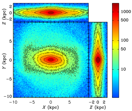
Figure 1: Face-on (center), end-on (right), and side-on (top) views of our simulated barred galaxy at a time of $2.4$ Gyr. Colors represent the surface density in arbitrary units. Black contours indicate $95\%$, $80\%$, $70\%$, $60\%$, $50\%$, and $40\%$ percent of the maximum surface density.

As a function of radius, Figure 2 shows the $m=2$ Fourier amplitudes of features in the density distribution that have well-defined frequencies, thus revealing coherent patterns and their pattern speeds (measured using several snapshots closely spaced temporarily around our selected time of $2.4$ Gyr; see Sparke & Sellwood 1987 for more details). The figure clearly shows that the bar has a constant intrinsic pattern speed $\Omega_{\rm p,int}=36.3$ km s^-1 kpc^-1 throughout its extent, while a pair of transient spiral arms with a lower pattern speed ($\Omega_{\rm p,spiral}=20.7$ km s^-1 kpc^-1) dominate the disk beyond the bar region.

Figure 2: Contours of the $m=2$ Fourier amplitudes of density distribution features as a function of radius and pattern speed, at our selected time of $2.4$ Gyr. The pattern speeds are derived from a Fourier analysis of the particles at a given radius as a function of time. The two dotted lines along the two prominent ridges represent the intrinsic pattern speeds of the bar ($\Omega_{\rm p,int}=36.3$ km s^-1 kpc^-1) and spiral arms ($\Omega_{\rm p,spiral}=20.7$ km s^-1 kpc^-1). For clarity, contours are from $5\%$ to $50\%$ of the maximum only, in steps of $5\%$. As expected, the strength of the bar feature decreases rapidly outside of the adopted bar (half-)length.

3.2 Mock data sets

At first, we align the simulated bar with the data $X_{\rm grid}$-axis, as shown in Figure 1. To create multiple mock data sets, the simulation is then rotated counterclockwise around the $Z_{\rm grid}$-axis by $\phi_{\rm bar}$, and inclined with respect to the $X_{\rm grid}$-axis (i.e., the major axis of the galaxy) by $i$, where $\phi_{\rm bar}$ ranges from $0\arcdeg$ to $180\arcdeg$ in steps of $5\arcdeg$ and $i$ ranges from $0\arcdeg$ to $90\arcdeg$ also in steps of $5\arcdeg$. We generally assume that the disk major axis is aligned with the $X$-axis of the grid (PA${}_{\rm disk}=90\arcdeg$), although we discuss the case where it is not in § 4.4.

After rotation, the simulated disk is placed at a distance of $100$ Mpc, typical of the MaNGA survey sample galaxies (Bundy et al., 2015). Assuming a stellar mass-to-light ratio $M/L=2$ ${\rm M}_{\sun}/{\rm L}_{\sun,r}$ at $r$ band, we then convert the projected mass to an $r$-band flux (or equivalently an $r$-band surface brightness $\Sigma$) map, with an original fine sampling (i.e., spaxel size) of $\approx 0\farcs 08$ or $40$ pc.

These finely binned flux maps are then convolved by a Gaussian PSF of variable width to mimic different seeings (i.e., different observing conditions). Our adopted PSF full widths at half maximum (FWHMs) range from $0\arcsec$ to $5\arcsec$ in steps of $0\farcs 5$, corresponding respectively to extremely good (e.g. adaptive optics) and bad seeings. After convolution, to generate realistic mock images, we further bin all the flux maps to match the Sloan Digitized Sky Survey (SDSS) imaging survey sampling size, and add the SDSS mean sky background and noise, resulting in a final coarse sampling (i.e., spaxel size) of $0\farcs 4$ or $200$ pc at $D=100$ Mpc (Gunn et al., 2006).

The creation of the required velocity fields is analogous to that of the flux maps, except for the convolution step. Indeed, unlike mass (i.e., flux), mean velocity is not a conserved quantity under convolution, but momentum is. Using the original fine grid, we therefore first calculate the mean LOS velocity $V_{||}$ in each spaxel and then multiply the resulting finely binned velocity map by the associated finely binned flux map, resulting in a finely binned map of the quantity $V_{||}\Sigma$. It is this map that we then convolve by the PSF, rather than the finely binned velocity map. The convolved finely binned $V_{||}\Sigma$ map is then more coarsely (re)binned as before and divided by the associated coarsely binned (and convolved) $\Sigma$ map to obtain the desired properly convolved coarsely binned $V_{||}$ map (see Eqs. 4 and 5).

In the end, we thus have mock flux (or surface brightness) and mean velocity maps with a range of relative bar angles $\phi_{\rm bar}$, inclinations $i$, and spatial resolutions (PSFs), all of which have a spaxel size of $200$ pc ($0\farcs 4$ at a distance of $100$ Mpc). Figure 3 shows examples of mock surface brightness and mean velocity maps with $\phi_{\rm bar}=45\arcdeg$, $i=45\arcdeg$, and two different seeings.

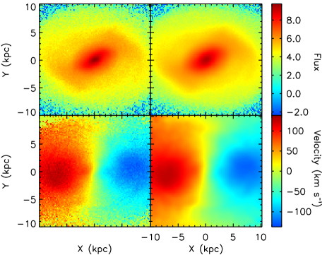
Figure 3: Mock surface brightness (top) and mean velocity (bottom) maps, for a relative bar angle $\phi_{\rm bar}=45\arcdeg$, an inclination $i=45\arcdeg$, no binning, and two different seeings of $0$ (left) and $2\arcsec$ (right).

3.3 Construction of Pseudo-slits

Pseudo-slits are positioned according to the projected disk orientation and bar length in the mock images. Most pseudo-slits are located within the bar region (in terms of their offset $Y$ from the galaxy major axis), but as the influence of a bar extends beyond its extent, we also locate a few extra pseudo-slits beyond the bar, to test whether these slits still yield accurate measurements of $\Omega_{\rm p}$. Moreover, the slit widths are varied from $0\farcs 4$ to $2\arcsec$ in steps of $0\farcs 4$, to investigate the slit width influence on the measurements. To obtain an independent measurement for each slit, adjacent pseudo-slits touch, but are not overlapped with, each other.

Figure 4 schematically shows how pseudo-slits are overlaid on mock images, for both the configuration used in most of the tests shown ($\phi_{\rm bar}=45\arcdeg$, $i=45\arcdeg$, and a slit width of $1\farcs 2$) and a configuration with narrower $0\farcs 4$ slits.

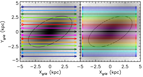
Figure 4: Examples of pseudo-slits schematically overlaid on mock images with $\phi_{\rm bar}=45\arcdeg$, $i=45\arcdeg$, and no binning. The width of the pseudo-slits is $1\farcs 2$ in the left panel and $0\farcs 4$ in the right panel. The colored straight lines schematically represent pseudo-slits with different offsets from the major axis (i.e., different $Y_{\rm grid}$ positions). Arrows indicate the positive direction of the pseudo-slits, while the open and filled circles denote pseudo-slits with respectively positive and negative offsets from the major axis, respectively.

In our study, as by construction the galaxy major axis is always aligned with the $X_{\rm grid}$-axis, we generally use easily constructed, perfectly rectangular horizontal slits, which are symmetric with respect to the minor axis (see the left panel of Fig. 5). However, as in practice the galaxy major axis (and thus the pseudo-slits) may be misaligned with respect to the axes of the data/grid, we also create pseudo-slits with irregular (zigzagged) asymmetric shapes, comprising only those spaxels whose center falls within the desired (perfectly rectangular) slit (see the right panel of Fig. 5). We then use those irregularly shaped pseudo-slits to test their effects (and the potential effects of recasting the grid) on TW $\Omega_{\rm p}$ measurements in §4.4.

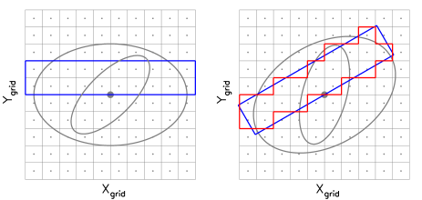
Figure 5: Schematic representations of pseudo-slits with different angles between the disk major axis and the data/grid axes (PA_disk). Gray grids and dots show respectively the spaxels and their centers, respectively. The large and small gray ellipses show respectively the (projected) disk and bar, respectively. Blue rectangles show the ideal, perfectly rectangular and symmetric pseudo-slits, which should always be parallel to the disk major axis for TW measurements. These are easily constructed in the left panel, where the disk major axis is aligned with the data/grid axes, but are awkward to construct in the right panel, where the disk is at an intermediate angle. The red rectangle in the right panel shows an irregularly shaped and asymmetric pseudo-slit, comprising only those spaxels whose center falls within the desired (perfectly rectangular) blue slit.

3.4 Determining $X_{\rm c}$ and $V_{\rm sys}$

Equation 1(a) suggests that an exact determination of the minor axis position ($X_{\rm c}$) and the galaxy systemic velocity ($V_{\rm sys}$) is very important for individual slit measurements and the TW averaging method. The center and mean velocity of our simulated galaxy are initially well determined (and by construction set to $0$), but thereafter the galaxy can shift slightly during its evolution. It is thus preferable to determine the value of $X_{\rm c}$ and $V_{\rm sys}$ from the chosen snapshot of the simulation itself. In fact, by measuring the mean position and velocity of our simulated galaxy in increasingly large volumes (centered on $0$), we see that they are indeed nearly $0$ up to a radius of $\approx 10$ kpc, but that significant offsets (like those discussed below in Fig. 6) exist when considering particles farther out, presumably because of “rogue”particles and asymmetries in the galaxy outer parts. Since most of the slits considered in our analyses do reach those distances, it appears essential to measure $X_{\rm c}$ and $V_{\rm sys}$ empirically from the simulation data.

Of course, an analogous determination of $X_{\rm c}$ and $V_{\rm sys}$ is likely to be essential for observational data, as they are unlikely to be known a priori and will need to be determined from the observational data themselves (i.e., a cube in the case of IFS data) or from ancillary imaging and spectroscopic data (see, e.g., Bureau et al., 1999).

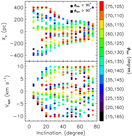
Figure 6: Minor axis position offset $X_{\rm c}$ (top panel) and systemic velocity offset $V_{\rm sys}$ (bottom panel) as a function of the bar orientation $\phi_{\rm bar}$ and inclination $i$ for a seeing of $2\arcsec$, no binning, and $\delta$PA${}_{\rm disk}=0\arcdeg$, as determined by minimizing the sum of the squares of the differences (of $\Omega_{\rm p}$ measurements) of opposite slit pairs. Results for $\phi_{\rm bar}<90\arcdeg$ and $\phi_{\rm bar}>90\arcdeg$ are shown as filled circles and squares, respectively.

Equation 1(a) suggests that if $X_{\rm c}$ and/or $V_{\rm sys}$ are wrong, slits with the same offset but on opposite sides of the galaxy major axis will yield $\Omega_{\rm p}$ measurements that are systematically (and increasingly) biased in opposite ways (i.e., respectively larger and smaller than the truth). To measure $X_{\rm c}$ and $V_{\rm sys}$ (for each bar orientation $\phi_{\rm bar}$, disk inclination $i$, and spatial resolution), we thus first measure $\Omega_{\rm p}$ for multiple slits (inner slits only; see § 4.2) and for a wide range of possible $X_{\rm c}$ and $V_{\rm sys}$ values and then select the $X_{\rm c}$ and $V_{\rm sys}$ (and associated $\Omega_{\rm p}$) that minimize the sum of the squares of the differences of opposite slit pairs (thus ensuring that the two slits in each pair yield $\Omega_{\rm p}$ measurements that are as similar to each other as possible).

We first let $X_{\rm c}$ and $V_{\rm sys}$ vary over a very wide range of values for every $(\phi_{\rm bar},i)$ pair. Most $X_{\rm c}$ and $V_{\rm sys}$ thus selected are small, as expected, but for extreme values of $\phi_{\rm bar}$ and $i$ the $X_{\rm c}$ and $V_{\rm sys}$ selected are nearly always at the extreme of the ranges allowed (no matter how large these are), and they often rapidly switch in an opposite manner from positive to negative values (suggesting that $X_{\rm c}$ and $V_{\rm sys}$ are somewhat degenerate, as expected from Eq. 1(a)). Since we will later discard those extreme $(\phi_{\rm bar},i)$ pairs as inappropriate for $\Omega_{\rm p}$ measurements (see § 4.6), in practice we restrict $X_{\rm c}$ and $V_{\rm sys}$ to smaller ranges appropriate for most $(\phi_{\rm bar},i)$ pairs ($-400~{}pc\leq X_{\rm c}\leq 400$ pc and $-10$ km s${}^{-1}\leq V_{\rm sys}\leq 10$ km s^-1).

Figure 6 shows the resulting $X_{\rm c}$ and $V_{\rm sys}$ offsets (with respect to $0$) as a function of $\phi_{\rm bar}$ and $i$ for a seeing of $2\arcsec$, no binning, and no position angle misalignment. Except for extreme values of $\phi_{\rm bar}$ and $i$, the systemic velocity offsets are nearly always small (generally $\lesssim 8$ km s^-1) and show no obvious trend. The results are similar for the minor axis position offsets, which can be large for extreme $(\phi_{\rm bar},i)$ pairs but are otherwise small (generally $\lesssim 1$ pixel and always $\lesssim 2$ pixels) and again show no clear trend. The increased minor axis position offsets at small $i$ are simply due to the deprojection (amplifying small offsets).

Importantly, Figure 7 shows that changes in $\Omega_{\rm p}$ when applying $X_{\rm c}$ and $V_{\rm sys}$ offsets are small (compared to measurements with no offset), $\lesssim 3\%$ excluding extreme $(\phi_{\rm bar},i)$ pairs, as expected from the fact that the simulation was centered to start with. Of course, the changes in the case of observational data are likely to be more significant, as a result of the poorer initial guesses for $X_{\rm c}$ and $V_{\rm sys}$.

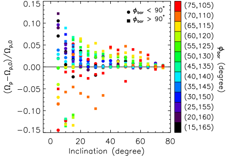
Figure 7: Fractional changes in $\Omega_{\rm p}$ measurements when applying $X_{\rm c}$ and $V_{\rm sys}$ offsets (compared to measurements with no offset, $\Omega_{\rm p,0}$), as a function of the bar orientation $\phi_{\rm bar}$ and inclination $i$ for a seeing of $2\arcsec$, no binning, and $\delta$PA${}_{\rm disk}=0\arcdeg$. Results for $\phi_{\rm bar}<90\arcdeg$ and $\phi_{\rm bar}>90\arcdeg$ are shown as filled circles and squares, respectively. Except for extreme $(\phi_{\rm bar},i)$ pairs, the changes are always $\lesssim 3\%$.

4 Results and Discussion

4.1 Integration along the Slits and Convergence Test

Ideally, the integrals in Equation 1(a) should range from $-\infty$ to $+\infty$, but this range is necessarily limited in real observations. As the integration limits (i.e., the length of each pseudo-slit) increase, measurements of $\Omega_{\rm p}$ based on Equation 1(a) should asymptotically converge and reach the true $\Omega_{\rm p}$ value at the (projected) radius where the disk becomes axisymmetric. It is thus very important to establish the minimum pseudo-slit length (i.e., the minimum spatial coverage) required for accurate TW measurements.

To establish this, we plot in Figure 8 distance (i.e., projected radius) profiles of the quantities $\int V_{||}\,\Sigma\,dX$ (the numerator of Eq. 1(a)), $\int X\,\Sigma\,dX$ (the denominator of Eq. 1(a)), and $\Omega_{\rm p}$ (the ratio of the numerator and denominator of Eq. 1(a) divided by the known $\sin i$), constructed by gradually increasing the (half-)slit length (i.e., the integration limits). Multiple pseudo-slits are shown, with different offsets from the disk major axis, for a mock data set with $\phi_{\rm bar}=45\arcdeg$, $i=45\arcdeg$, $2\arcsec$ seeing, $1\farcs 2$ slit width, no binning, and $\delta$PA${}_{\rm disk}=0\arcdeg$.

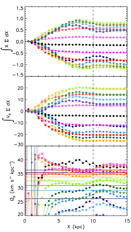
Figure 8: Example convergence test. From top to bottom, the panels show distance (i.e., projected radius) profiles of the quantities $\int V_{||}\,\Sigma\,dX$, $\int X\,\Sigma\,dX$, and $\Omega_{\rm p}$ (see Eq. 1(a)), constructed by gradually increasing the slit (half-)length (i.e., the integration limits). For display purposes, the profiles in the upper and middle panels also are normalized by the total flux in each slit. Data points with different colors show pseudo-slits with different offsets from the simulated galaxy major axis (increasing from magenta to dark blue; see Fig. 4), with open and filled circles showing slits with the same offset but on, respectively, the positive and negative side of the major axis (see Fig. 4). The thick gray solid horizontal line shows the intrinsic bar pattern speed of the simulated galaxy ($\Omega_{\rm p,int}=36.3$ km s^-1 kpc^-1). The other dotted and solid colored horizontal lines indicate the associated weighted bar pattern speeds from Equation 6, for, respectively, positive and negative offsets from the major axis. The gray dashed vertical lines indicate a distance of $10$ kpc, where by convention we take our $\Omega_{\rm p}$ measurements. The mock data set used in this test has $\phi_{\rm bar}=45\arcdeg$, $i=45\arcdeg$, $2\arcsec$ seeing, $1\farcs 2$ slit width, no binning, and $\delta$PA${}_{\rm disk}=0\arcdeg$.

As alluded to above, for ease of interpretation and comparison to the known intrinsic bar pattern speed $\Omega_{\rm p,int}=36.3$ km s^-1 kpc^-1, in Figure 8 and all other figures and measurements in this section we divide each $\Omega_{\rm p}\sin i$ measurement by $\sin i$ using the known inclination (i.e., the inclination with which the simulation was projected). For real observations, the accuracy with which an $\Omega_{\rm p}\sin i$ measurement can be deprojected clearly depends on the accuracy of the measured inclination, adding an additional uncertainty to the $\Omega_{\rm p}$ measurement.

Figure 8 shows that $\int V_{||}\,\Sigma\,dX$ and $\int X\,\Sigma\,dX$ have converged by a distance of $\approx 8$ kpc ($\approx 3.3$ $R_{\rm e}$ for our simulated galaxy, much larger than the bar half-length), where convergence is defined here as being within $10\%$ of the known true value. However, somewhat surprisingly, $\Omega_{\rm p}$ converges much earlier, by a distance of $\approx 3$ kpc ($\approx 1.3$ $R_{\rm e}$, slightly shorter than the projected bar half-length). The convergence distance for $\int V_{||}\,\Sigma\,dX$ and $\int X\,\Sigma\,dX$ is thus a rather conservative estimate of the required slit (half-)length, and a much smaller field coverage is sufficient for reliable TW $\Omega_{\rm p}$ measurements.

While Figure 8 shows the convergence test for a single $(\phi_{\rm bar},i)$ pair, convergence tests for the entire range of $\phi_{\rm bar}$ and $i$ yield similar results, i.e., while the convergence distances of the two integrals taken separately (numerator and denominator of Eq. 1(a)) are always rather large (and slightly larger for smaller $\phi_{\rm bar}$), the convergence distance of their ratio (i.e., $\Omega_{\rm p}$) is always much smaller (and remains essentially unchanged). Guo et al. (2019) also tested the influence of the slit (half-)length on TW measurements and found that $\Omega_{\rm p}$ distance profiles converge by $\approx 1.2$ times the bar half-length. The convergence distances are similar for different inclinations and bar orientations.

Having said that, the convergence distance is likely to differ from galaxy to galaxy, and $\Omega_{\rm p}$ distance profiles may never converge in the presence of large-scale asymmetries such as spiral arms and lopsidedness. We therefore recommend to checking whether the $\Omega_{\rm p}$ distance profiles converge on a slit-by-slit and galaxy-by-galaxy basis. Only those slits where $\Omega_{\rm p}$ has converged yield reliable bar pattern speed measurements.

Here, for simplicity, we adopt as the pattern speed measured for one slit the value at a distance of $10$ kpc (i.e., the absolute value of the integration limits and thus the half-slit length), well beyond the convergence distance of any slit.

4.2 Pseudo-slit Selection

The different colors in Figure 8 show pseudo-slits with different offsets from the simulated galaxy major axis (or, equivalently, different $Y_{\rm grid}$ positions), while open and filled circles show slits with the same offset but on opposite sides of the major axis. Except for the three outermost pseudo-slits, all other pseudo-slits (which we will refer to as inner slits) are located within the bar region. The three panels of Figure 8 show that the distance profiles of the outer slits have significant fluctuations, much greater than those of the inner slits. In particular, the (absolute) values of the profiles can decrease with radius. Most importantly, the bottom panel of Figure 8 shows that, as the offset from the major axis increases, all slits yield a systematically and increasingly biased measurement of $\Omega_{\rm p}$ (toward lower values), with the three outer slits significantly worse. This is likely due to the two transient spiral arms with a lower pattern speed in the outer parts of the simulated disk (see Fig. 2). Indeed, beyond the bar ends, the contribution of the bar to the pattern becomes less significant and the spiral arms begin to dominate. It is thus important to quantify this effect to ascertain the reliability of TW $\Omega_{\rm p}$ measurements using increasingly offset pseudo-slits.

To investigate the effects of the spiral arms on the bar pattern speed measurements, we compute a simple weighted measure of $\Omega_{\rm p}$ ($\Omega_{\rm p,weighted}$), by weighting the bar and spiral arm pattern speeds by their likely contributions to the integrals in Equation 1(a). We thus calculate the luminosity within and beyond the (projected) bar region along each pseudo-slit and then weight the two pattern speeds accordingly, i.e.,

$$\Omega_{\rm p,weighted}\equiv\frac{\Sigma_{\rm bar}\,\Omega_{\rm p,bar}+\Sigma_{\rm spiral}\,\Omega_{\rm p,spiral}}{\Sigma_{\rm bar}+\Sigma_{\rm spiral}}\,\,\,,$$ (6)

where $\Omega_{\rm p,bar}=\Omega_{\rm p,int}=36.3$ km s^-1 kpc^-1, $\Omega_{\rm p,spiral}=20.7$ km s^-1 kpc^-1 (see Fig. 2), and $\Sigma_{\rm bar}$ and $\Sigma_{\rm spiral}$ are the fluxes respectively within and beyond the bar region, respectively. The bar region is defined here as the elliptical region with an ellipticity equal to the maximum bar ellipticity ($\epsilon_{\rm bar,max}=0.47$) and a semi-major-axis radius equal not to the bar half-length ($a_{\rm bar}=4.6$ kpc), but rather to the radial extent of the main feature with a pattern speed equal to that of the bar in Figure 2 ($8$ kpc).

The resulting weighted pattern speeds are shown as horizontal lines in the bottom panel of Figure 8, appropriately colored for each pseudo-slit (dotted and solid lines denote pseudo-slits with, respectively, positive and negative offsets from the major axis; see Fig. 4). As expected, the figure shows that $\Omega_{\rm p,weighted}$ systematically decreases with increasing major axis offset. Most importantly, $\Omega_{\rm bar,weighted}$ roughly agrees with the TW measurement for all the slits, and it slowly tends to $\Omega_{\rm p,spiral}\approx 21$ km s^-1 kpc^-1 for the three outer slits. This indicates that pseudo-slits located outside the bar region will not yield accurate TW $\Omega_{\rm p}$ measurements (as outer spiral arms increasingly bias the measurements), in turn suggesting that only pseudo-slits located within the bar region should be used.

Figure 9 shows a comparison of the TW $\Omega_{\rm p}$ measurements for the different slits and for appropriate slit averages. In the left panel, the TW averaging method is used, whereby each measurement shown is the average of that for multiple pseudo-slits. The gray solid line shows the known intrinsic pattern speed of the bar in the simulated galaxy ($\Omega_{\rm p,int}=36.3$ km s^-1 kpc^-1), while each colored solid line shows the average pattern speed of all the slits within a given offset from the galaxy major axis (i.e., all slits within a given minor axis position $|Y_{\rm grid}|$), identified by the large circles of the same color. Again, we see that the average $\Omega_{\rm p}$ decreases as slits with increasingly large offsets from the major axis are used. In the test shown, the adopted TW $\Omega_{\rm p}$ measurement would be $>5\%$ lower than the real value when all pseudo-slits are used, and $\approx 5\%$ too low when only the inner pseudo-slits are used.

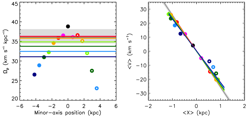
Figure 9: Individual and average bar pattern speed measurements using the TW averaging (left) and the TW fitting (right) method. The data points are as in Figure 8. The gray solid lines show the intrinsic pattern speed of the bar, and all measurements within the pale gray regions have relative errors $\leq 5\%$. Each colored line in the left (right) panel shows the average pattern speed (the fit to the $<V>$ vs. $<X>$ data points) of all the slits within a given offset from the galaxy major axis (i.e., all slits within a given minor axis position), identified by the large circles of the same color. The mock data set used in this test has $\phi_{\rm bar}=45\arcdeg$, $i=45\arcdeg$, $2\arcsec$ seeing, $1\farcs 2$ slit width, no binning, and $\delta$PA${}_{\rm disk}=0\arcdeg$.

The right panel of Figure 9 shows an analogous comparison of the TW $\Omega_{\rm p}$ measurements when the TW fitting method is used instead. Here $<V>$ and $<X>$ are calculated for each pseudo-slit, and each adopted $\Omega_{\rm p}$ is obtained from the fitted slope to the ($<V>$ vs. $<X>$) data points within a given offset from the galaxy major axis (again color-coded). The results are consistent with those of the TW averaging method, the fitted slope decreasing by a similar fraction as slits increasingly offset from the major axis are incorporated into the fit. The right panel of Figure 9 also shows that the (absolute) values of $<V>$ and $<X>$ decrease for the outer slits (after peaking for the pseudo-slits closest to the bar ends).

Compared to the inner slits, we thus see from Figures 8 and 9 that the distance profiles, measurement errors, and $<V>$ – $<X>$ diagrams of the outer slits behave differently than those of the inner slits. In addition to an actual bar (half-)length measurement, these behaviors can help us to distinguish the inner and outer slits, and thus to select the appropriate pseudo-slits for a TW $\Omega_{\rm p}$ measurement. Whether using the TW averaging or the TW fitting method, we therefore recommend using only pseudo-slits located within the bar region.

4.3 Spatial Binning

To test the effect of spatial binning, we bin the mock images over multiple spaxels using the commonly used Voronoi binning algorithm of Cappellari & Copin (2003). Differently from real observations, the noise is defined here as the Poisson noise of the total flux within each bin. The spaxels within each bin are labeled, and the surface brightness and velocity of the bin are then replaced by their (luminosity-weighted) spatial averages. Figure 10 shows binned flux and mean velocity maps with different S/N thresholds. Given the necessarily different S/N definitions, it is not possible to directly compare the S/N estimates of real observations with ours, so we use instead the total number of bins within the field of view to characterize the severity of the binning applied (more severe binning, or equivalently higher S/N thresholds, leading to fewer and larger bins). We tested the sensitivity of both the TW averaging method and the TW fitting method to binning, and both yield consistent results.

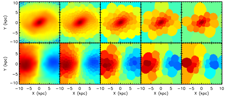
Figure 10: Examples of binned flux (top) and mean velocity (bottom) maps generated using the Voronoi binning algorithm. From left to right, the target S/N (number of bins) of the Voronoi bins is $0$ ($10101$; no binning), $50$ ($516$), $100$ ($142$), $150$ ($64$), and $200$ ($36$). The mock images have $\phi_{\rm bar}=45\arcdeg$, $i=45\arcdeg$, and $2\arcsec$ seeing.

Figure 11 shows the relative error of the bar pattern speed measurement ($\Delta\Omega_{\rm p}/\Omega_{\rm p,int}$) as a function of the number of bins for the TW averaging method, for a range of viewing angles. The FOV of the mock images is $20\times 20$ kpc² in all cases. As expected, when the number of bins is large (here $\gtrsim 200$, i.e., little binning or low S/N threshold), spatial binning has no effect on the $\Omega_{\rm p}$ measurements (independently of the viewing angle). Interestingly, the relative $\Omega_{\rm p}$ error does not increase monotonically with the number of bins when the number of bins is decreased; it changes abruptly when the number of bins is sufficiently small (here $\lesssim 200$). This is probably a direct consequence of the importance of the bins’ positions and shapes to the TW integrals. The results of the TW integrals will be very different for pseudo-slits intersecting, e.g., a few small bin centers versus the boundaries of several large bins. Overall, Figure 11 shows a general trend of increasing (absolute value of the) relative error $\Delta\Omega_{\rm p}/\Omega_{\rm p,int}$ with decreasing number of bins (i.e., more aggressive binning or higher S/N thresholds) when the number of bins is sufficiently small. The bar pattern speed $\Omega_{\rm p}$ is then almost always underestimated, by as much as $15\%$ for the most severe binning considered.

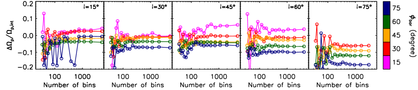
Figure 11: Spatial binning test. The relative $\Omega_{\rm p}$ error is shown as a function of the number of bins for different inclinations $i$ (from left to right) and bar angles $\phi_{\rm bar}$ (colors). The bar pattern speeds $\Omega_{\rm p}$ are measured using the TW averaging method. All the mock images used in this test have an FOV of $20\times 20$ kpc², $2\arcsec$ seeing, $1\farcs 2$ slit width, and $\delta$PA${}_{\rm disk}=0\arcdeg$.

From Figure 11, we can draw the conclusion that binned IFS data with a number of bins smaller than $\approx 200$ in an FOV of $20\times 20$ kpc² should be discarded for TW $\Omega_{\rm p}$ measurements.

4.4 Grid Recasting

As shown in the right panel of Figure 5, when the major axis of the disk is misaligned from the data/grid axes, the integrations along the (pseudo-)slits required for TW measurements (see Eq. 1(a)) are nontrivial. Naively, one can simply integrate (i.e., sum) along an irregularly shaped slit comprising only those spaxels whose center falls within the desired (perfectly rectangular) slit (see the red polygon in the right panel of Fig. 5). Alternatively, one can recast (i.e., regrid) the grid to align the galaxy major axis with the $X_{\rm grid}$-axis (see the blue rectangle in the left panel of Fig. 5), or equivalently carry out a more complex summation along the slit (see the blue rectangle in the right panel of Fig. 5).

To quantify the potential biases associated with summing along irregularly shaped slits and/or the recasting process, we create new mock data sets where the disk major axis is misaligned from the $X_{\rm grid}$-axis. Specifically, after projection, we further rotate the model counterclockwise, so that the angle between the disk major axis and the data/grid axes (PA_disk) ranges from $0\arcdeg$ to $90\arcdeg$ in steps of $5\arcdeg$, this for all $\phi_{\rm bar}$ and $i$.

To simulate the effects of recasting, we subsequently also recast (i.e., rotate and regrid) all the above mock data sets to align the disk major axis with the $X_{\rm grid}$-axis. To achieve this, we apply a bilinear interpolation to the surface brightness ($\Sigma$) maps directly. Analogously to the convolutions described in § 3.2, however, we first multiply the velocity fields $V_{||}$ by their associated surface brightness maps $\Sigma$ to obtain $V_{||}\Sigma$ maps. We then apply the bilinear interpolation to these $V_{||}\Sigma$ maps and divide the recast $V_{||}\Sigma$ maps by their associated recast $\Sigma$ maps, to finally obtain the desired recast velocity field $V_{||}$. All the recast mock surface brightness maps and velocity fields then have the disk major axis aligned with the $X_{\rm grid}$-axis, and the pseudo-slits constructed are perfectly rectangular, symmetric with respect to the minor axis, and parallel to the $X_{\rm grid}$-axis (see the left panel of Fig. 5).

TW $\Omega_{\rm p}$ measurements are then carried out on the two sets of simulated data, those recast and those with irregularly shaped slits. These $\Omega_{\rm p}$ measurements are then compared to each other and to the known intrinsic bar pattern speed of the simulated galaxy ($\Omega_{\rm p,int}=36.3$ km s^-1 kpc^-1) in Figure 12, for mock data sets with $i=45\arcdeg$, a range of $\phi_{\rm bar}$, $2\arcsec$ seeing, $0.4$ and $1\farcs 2$ slit widths, no binning, $\delta$PA${}_{\rm disk}=0\arcdeg$, and for both the TW averaging and TW fitting methods. Measurements carried out without recasting (i.e., with irregularly shaped slits) and with recasting (i.e., perfectly rectangular slits) are shown side by side for comparison.

Figure 12: Grid recasting test. TW $\Omega_{\rm p}$ measurements are shown as a function of PA_disk, the angle between the galaxy major axis and the data/grid axes (specifically $Y_{\rm grid}$), for data sets without (first and third columns) and with (second and fourth columns) grid recasting. No recasting is required for PA${}_{\rm disk}=0$ and/or $90\arcdeg$. From top to bottom and left to right, $\phi_{\rm bar}$ increases from $15\arcdeg$ to $165\arcdeg$ in steps of $15\arcdeg$. Measurements using the TW averaging and fitting method are shown, respectively, as filled circles and stars. The gray solid horizontal lines show the intrinsic $\Omega_{\rm p}$ of the simulated galaxy ($\Omega_{\rm p,int}=36.3$ km s^-1 kpc^-1). The mock data sets used in this test have $i=45\arcdeg$, $2\arcsec$ seeing, $0.4$ (black data points) and $1\farcs 2$ (red data points) slit widths, no binning, $\delta$PA${}_{\rm disk}=0\arcdeg$, and a range of $\phi_{\rm bar}$.

Comparing the naive integrations along irregularly shaped slits and recast measurements (i.e.,  each pair of panels in Fig. 12), Figure 12 shows that the two sets of measurements are consistent. However, the recast measurements always show less scatter. Indeed, the relative difference between the measurements $\Delta\equiv|\Omega_{\rm p,max}-\Omega_{\rm p,min}|/\Omega_{\rm p,int}$ is then $\lesssim 2\%$ for both narrow and wide slits, where $\Omega_{\rm p,max}$ and $\Omega_{\rm p,min}$ are, respectively, the maximum and minimum derived $\Omega_{\rm p}$ at a given $\phi_{\rm bar}$. The relative difference $\Delta$ can be as large as $7\%$ for narrow and wide slits before the recasting process. Simulated galaxies at different inclinations show the same trends. This suggests that naive integrations with irregularly shaped slits do affect TW $\Omega_{\rm p}$ measurements, presumably due to the asymmetries introduced (and removed by recasting the grid, so that the only asymmetries left are those due to the bar itself, as required by TW). Recasting the grid (or, equivalently, carrying out a more complex summation along the slits) should thus help to reduce measurement uncertainties.

Interestingly, Figure 12 shows that, for any given $\phi_{\rm bar}$, the TW $\Omega_{\rm p}$ measurements do not systematically depend on PA_disk, which simply introduces a little bit of scatter in the measurements. This is reassuring and confirms the suggestion above that a misalignment of the galaxy major axis from the data/grid axes (and potential associated recasting effects) does not significantly impact TW $\Omega_{\rm p}$ measurements with IFSs. However, grid recasting does help to decrease the scatter of TW measurements with PA_disk.

Figure 12 also reveals that the TW fitting and TW averaging methods generally share the same trends. However, the TW fitting method systematically yields slightly lower TW $\Omega_{\rm p}$ measurements than the TW averaging method, the difference increasing with increasing $\phi_{\rm bar}$. This is somewhat surprising, as one would naively expect the TW fitting method to be superior to the TW averaging method. We do not fully understand this tendency, but it seems to be related to the aforementioned fact that the $\Omega_{\rm p}$ measurements decrease with increasing offset from the major axis. Indeed, the inner slits near the ends of the bar (i.e., the green datapoints in the right panel of Fig. 9) yield both the lowest $\Omega_{\rm p}$ estimates and the greatest (absolute) values of $<V>$ and $<X>$, thus effecting the greatest leverage (down) on $\Omega_{\rm p}$ when fitting the straight line. This in turn yields lowered estimates compared to ones with effectively equal weight for all datapoints. This effect becomes more acute for larger $\phi_{\rm bar}$ as the intersection of the bar and the slit decreases, and it can be minimized by neglecting the slits near the ends of the bar.

In any case, most importantly here, even after recasting Figure 12 shows that the scatter across the measurements is most significant at small $\phi_{\rm bar}$ (i.e., $\phi_{\rm bar}\lesssim 15\arcdeg$; both $\phi_{\rm bar}\lesssim 15\arcdeg$ and $75\arcdeg\lesssim\phi_{\rm bar}\lesssim 105\arcdeg$ before recasting). The relative difference $\Delta\approx 2\%$ when $\phi_{\rm bar}\gtrsim 15\arcdeg$, but it can be as large as $7\%$ for $\phi_{\rm bar}\lesssim 15\arcdeg$ and $11\%$ for $75\arcdeg\lesssim\phi_{\rm bar}\lesssim 105\arcdeg$ before recasting. This suggests that bar pattern speed measurements of galaxies with disadvantageous $\phi_{\rm bar}$ will have large uncertainties, and that these galaxies should be excluded from observational samples. In § 4.6, we shall therefore explore the optimal range of both $\phi_{\rm bar}$ and $i$ for sample selection.

4.5 Disk Position Angle

4.5.1 Pattern Speed Uncertainties

To quantify the effects of misalignments ($\delta$PA_disk) of the (pseudo-)slits with respect to the true position angle of the disk (PA_disk), we must create new mock images. As described in § 3.2, the simulated bar is normally first aligned with the data $X_{\rm grid}$-axis, and the disk is then rotated about the $Z_{\rm grid}$-axis counterclockwise by $\phi_{\rm bar}$ and about the $X_{\rm grid}$-axis by $i$. After these two rotations, the disk major axis lies along the $X_{\rm grid}$-axis by construction. To introduce a misalignment of the pseudo-slits, we further rotate the disk about the $Z_{\rm grid}$-axis by an angle $\delta$PA_disk (but continue to assume that the disk major axis is along the $X_{\rm grid}$-axis for the purpose of the TW calculations). For these tests, $i$ and $\phi_{\rm bar}$ range from $15\arcdeg$ to $165\arcdeg$ in steps of $15\arcdeg$ and $\delta$PA_disk ranges from $-10\arcdeg$ to $10\arcdeg$ in steps of $1\arcdeg$. By convention (and as in D03), $\delta$PA${}_{\rm disk}>0$ when the true disk major axis is rotated anticlockwise. For $\phi_{\rm bar}\lesssim 90\arcdeg$, the additional rotation increases the angle between the bar and the assumed major axis (i.e., the $X_{\rm grid}$-axis), while for $\phi_{\rm bar}\gtrsim 90\arcdeg$ the additional rotation decreases that angle. We carry out this test using both the TW averaging method and the TW fitting method, but the results are very similar. The relative $\Omega_{\rm p}$ errors introduced by position angle misalignments are thus shown in Figure 13 for the TW averaging method only.

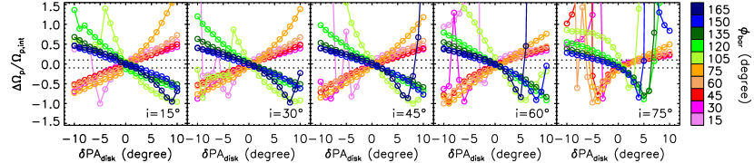
Figure 13: Position angle test. The relative $\Omega_{\rm p}$ error is shown as a function of the position angle misalignment angle $\delta$PA_disk for different inclinations $i$ (from left to right) and bar angles $\phi_{\rm bar}$ (colors). The black dotted horizontal lines mark relative errors of $\pm 10\%$. The bar pattern speeds $\Omega_{\rm p}$ are measured using the TW averaging method. The mock data sets used in this test have a $2\arcsec$ seeing, $1\farcs 2$ slit width, and no binning.

Figure 13 confirms the result of D03 that not only are position angle misalignments the most important factor potentially affecting TW $\Omega_{\rm p}$ measurements, but their effect is also systematic. Indeed, Figure 13 suggests that the (absolute value of the) relative error $\Delta\Omega_{\rm p}/\Omega_{\rm p,int}$ is $\approx 35\%$ for all inclinations $i$ and most bar angles $\phi_{\rm bar}$ when the misalignment angle is as small as $5\arcdeg$. When $75\lesssim\phi_{\rm bar}\lesssim 105\arcdeg$, the relative $\Omega_{\rm p}$ errors can be very large for even smaller $\delta$PA_disk. In fact, when $\delta$PA${}_{\rm disk}\approx 10\arcdeg$, $\Delta\Omega_{\rm p}/\Omega_{\rm p,int}$ can reach $100\%$. This test thus suggests that the measured $\Omega_{\rm p}$ can be severely overestimated when the angle between the bar and the assumed disk major axis is wrongly increased, while it can be severely underestimated when that angle is decreased.

We note that D03 also examined the effects of position angle misalignment on TW $\Omega_{\rm p}$ measurements. He used a simulated barred galaxy with $i=45\arcdeg$ and $\phi_{\rm bar}=30\arcdeg,45\arcdeg$ and $60\arcdeg$ (his Figure 9), which can be directly compared with our tests. The results are analogous, except that our relative errors are slightly smaller, probably due to differences in the simulated galaxies.

4.5.2 Empirical Diagnostic

Given the importance of identifying the true disk position angle PA_disk to avoid the substantial systematic biases just described, it would be very useful to have an empirical diagnostic of it, i.e., a method to identify or measure the true disk position angle from the data themselves. In this subsection, we therefore explore such empirical diagnostics, unfortunately only with partial success.

We test three different parameters (scatters) to quantify the “goodness” of the position angle used: (a) the sum of the squares of the differences of opposite slit pair measurements, (b) the sum of the squares of the differences of all slit measurements with respect to the mean (i.e., the scatter across all pseudo-slit measurements), and (c) the sum of the previous two parameters. We define the goodness of a given position angle as $\left[1-\frac{(\sigma-\sigma_{\rm min})}{(\sigma_{\rm max}-\sigma_{\rm min})}\right]$, where $\sigma$ is the given measure of scatter evaluated at that position angle and $\sigma_{\rm min}$ and $\sigma_{\rm max}$ are, respectively, the minimum and maximum scatter measured within the entire position angle ranged probed. This goodness ranges from $0$ to $1$ by definition, with the maximum value ($1$) defining what naively would appear to be the most appropriate disk position angle to use. We compare the goodness of a range of $\delta$PA_disk for a number of $(\phi_{\rm bar},i)$ pairs (and for each of the three scatters defined) in Figure 14.

We naively expected the goodness to be maximum ($1$) for $\delta$PA${}_{\rm disk}=0\arcdeg$, thus allowing us to empirically identify the true position angle when it is not accurately known a priori. However, Figure 14 reveals the situation to be more complex. First, the maximum of the first parameter tested (a, red curves) is often not very well defined. Second, even for the second (b, green curves) and third (c, blue curves) parameters tested, although a clear maximum is often present near $\delta$PA${}_{\rm disk}=0\arcdeg$, it is often away from exactly $\delta$PA${}_{\rm disk}=0\arcdeg$ (nevertheless suggesting that the second parameter, the scatter across all inner pseudo-slits, is the most promising diagnostic tested). Indeed, the peaks in the goodness profiles of the second and third parameters often deviate from $\delta$PA${}_{\rm disk}=0\arcdeg$ by a few degrees ($\lesssim 5\arcdeg$) when $i\lesssim 60\arcdeg$ (the goodness profiles for $i=75\arcdeg$ are uninformative). When $\phi_{\rm bar}=45\arcdeg$, the true disk position angle is accurately recovered (i.e., the goodness is maximum for $\delta$PA${}_{\rm disk}\approx 0\arcdeg$). However, when the bar is close to the disk major axis ($\phi_{\rm bar}<45\arcdeg$), the suggested disk position angle is always slightly larger than the truth (i.e., the goodness is maximum for $\delta$PA${}_{\rm disk}>0\arcdeg$). Conversely, when the bar is close to the disk minor axis ($\phi_{\rm bar}>45\arcdeg$), the suggested disk position angle is always smaller than the truth (i.e., the goodness is maximum for $\delta$PA${}_{\rm disk}<0\arcdeg$). Given the sensitivity of $\Omega_{\rm p}$ to a disk position angle error of even a few degrees (see the previous § 4.5.1), these diagnostics are simply not good enough.

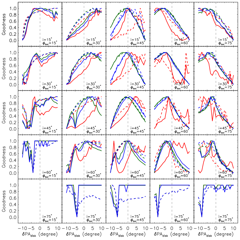
Figure 14: Empirical diagnostics of the true disk position angle. The goodness of the parameter is shown as a function of $\delta$PA_disk for a range of bar angles $\phi_{\rm bar}$ (increasing from left to right in steps of $15\arcdeg$) and inclinations $i$ (increasing from top to bottom in steps of $15\arcdeg$), this for the three parameters discussed in the text: sum of the squares of the differences of opposite slit pair measurements (a, red), sum of the squares of the differences of all slit measurements with respect to the mean (b, green), and sum of the previous two parameters (c, blue). The goodness ranges from $0$ to $1$ by definition. Solid (dashed) lines show the goodness when applying ( not applying) $X_{\rm c}$ and $V_{\rm sys}$ offsets.

While showing some promise, the potential empirical diagnostics of the true disk position angle presented in Figure 14 thus fall short of what is required to ensure bar pattern measurements devoid of significant PA_disk-related systematic errors. We also do not fully understand the systematic dependence of the goodness adopted on the bar angle $\phi_{\rm bar}$. Further investigations are thus required to identify a more reliable empirical diagnostic of the true disk position angle.

4.6 Bar Orientation and Inclination

As discussed in § 2.1 (and according to Eq. 1(a)), the TW integrals will sum to $\approx 0$ if a bar is nearly parallel ($\phi_{\rm bar}=0\arcdeg$) or perpendicular ($\phi_{\rm bar}=90\arcdeg$) to the major axis of the disk. In addition, the LOS velocities will be very small (and undistinguishable within the uncertainties) if a galaxy is close to face-on ($i=0\arcdeg$), while a bar will be difficult to identify if a galaxy is close to edge-on ($i=90\arcdeg$). It is thus necessary to exclude those galaxies with disadvantageous $\phi_{\rm bar}$ and $i$ for reliable TW $\Omega_{\rm p}$ measurements.

There is no specific prescription for the optimal $\Omega_{\rm p}$ ranges, so we use our simulated galaxy with different projections to identify those optimal ranges here. To do this, we will consider two quantities. First, the relative difference of each average $\Omega_{\rm p}$ measurement with respect to the known intrinsic bar pattern speed ($\Omega_{\rm p,int}=36.3$ km s^-1 kpc^-1), where the TW average is taken over all individual inner slit measurements of a given $(\phi_{\rm bar},i)$ pair. Second, the relative uncertainty of each average $\Omega_{\rm p}$ measurement with respect to the known intrinsic bar pattern speed, where the uncertainty is defined as the root mean square (rms) scatter across all individual inner slit measurements of a given $(\phi_{\rm bar},i)$ pair.

We note that there are very few inner pseudo-slits when $\phi_{\rm bar}\lesssim 10\arcdeg$ (or $\phi_{\rm bar}\gtrsim 170\arcdeg$) and/or the disk is nearly edge-on, as the bar is then nearly parallel to the major axis of the disk and/or the projected bar length is too short. By the time $i\approx 90\arcdeg$ is reached, measurements are essentially impossible for any $\phi_{\rm bar}$. In particular, the uncertainty measure defined above requires at least two slits.

Figure 15 shows the (absolute values of the) $\Omega_{\rm p}$ relative differences and uncertainties derived from mock data sets with a $2\arcsec$ seeing, $1\farcs 2$ slit width, no binning, $\delta$PA${}_{\rm disk}=0\arcdeg$, and a range of $\phi_{\rm bar}$ and $i$. From the figure, we see that the relative differences are $\gtrsim 10\%$ when $\phi_{\rm bar}\lesssim 10\arcdeg$ and $75\arcdeg\lesssim\phi_{\rm bar}\lesssim 105\arcdeg$, or $i\lesssim 15\arcdeg$ and $i\gtrsim 70\arcdeg$. Similarly, the relative uncertainties are $\gtrsim 10\%$ for $75\arcdeg\lesssim\phi_{\rm bar}\lesssim 105\arcdeg$ or $i\lesssim 15\arcdeg$. In any case, it is difficult to accurately measure the inclination of a nearly face-on galaxy, as the disk appears nearly (but may not be intrinsically perfectly) round, and the deprojection correction to the velocities (or equivalently the $\Omega_{\rm p}\sin i$ TW measurement) is very large. The projection of the bar on the minor axis is also too short to construct multiple pseudo-slits when $\phi_{\rm bar}$ is small.

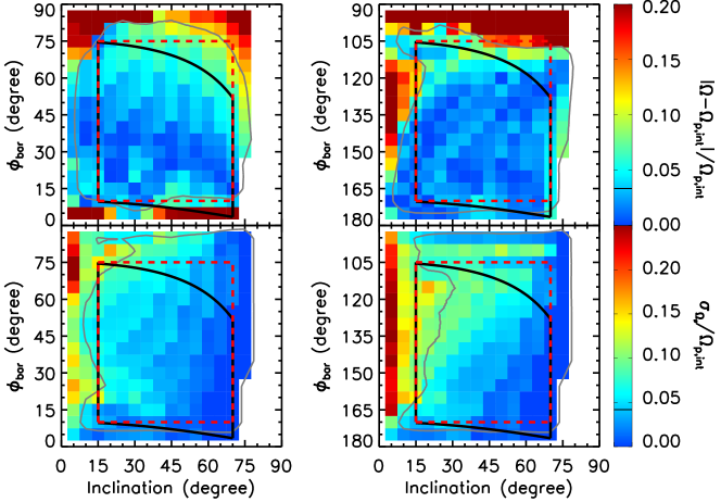
Figure 15: Optimal $\phi_{\rm bar}$ and $i$ range test for $\phi_{\rm bar}\leq 90\arcdeg$ (left panels) and $\phi_{\rm bar}\geq 90\arcdeg$ (right panels). Colors in the top panels show the (absolute value of the) relative difference of each average $\Omega_{\rm p}$ measurement (with respect to the known intrinsic bar pattern speed $\Omega_{\rm p,int}=36.3$ km s^-1 kpc^-1) as a function of $\phi_{\rm bar}$ and $i$, where the average is taken over all individual inner slit measurements. Colors in the bottom panels show the relative uncertainty of each average $\Omega_{\rm p}$ measurement, defined as the ratio of the rms scatter across all individual inner slit measurements to the known intrinsic bar pattern speed $\Omega_{\rm p,int}=36.3$ km s^-1 kpc^-1. White regions indicate $(\phi_{\rm bar},i)$ pairs inappropriate for TW $\Omega_{\rm p}$ measurements ($i=0\arcdeg$, $\phi_{\rm bar}=0$ or $180\arcdeg$, single inner slit). Solid gray lines are $10\%$ contours. The red dashed box identifies the optimal intrinsic ($\phi_{\rm bar}$, $i$) region (as used throughout this paper), while the black box identifies the optimal observed ($\phi_{\rm bar,obs}$, $i$) region (see Footnote 2). The optimal observed $\phi_{\rm bar,obs}$ range (black box) should be used when selecting samples for TW measurements. The mock data sets used in this test have $2\arcsec$ seeing, $1\farcs 2$ slit width, no binning, $\delta$PA${}_{\rm disk}=0\arcdeg$, and a range of $\phi_{\rm bar}$ and $i$.

As already mentioned, according to Eq. 1(a), the TW integrals will sum to $\approx 0$ if a bar is nearly parallel ($\phi_{\rm bar}=0\arcdeg$) or perpendicular ($\phi_{\rm bar}=90\arcdeg$) to the major axis of the disk. The $\Omega_{\rm p}$ inferred is then expected to have large uncertainties. Figure 15 indeed suggests that the relative differences are very large when $\phi_{\rm bar}\approx 90\arcdeg$, but surprisingly the relative differences remain small for $\phi_{\rm bar}\approx 0\arcdeg$ (or, equivalently, $\phi_{\rm bar}\approx 180\arcdeg$). To investigate this, we show in Figure 16 the TW $\Omega_{\rm p}$ measurements for individual pseudo-slits (and their averages), for a range of bar angles $\phi_{\rm bar}$ and inclinations $i$. Figure 16 reveals a clear systematic dependence of the measurements on the bar orientation. The relatively good quality of the measurements when $\phi_{\rm bar}\approx 0\arcdeg$ is confirmed. However, unexpectedly, not only are the measurements poor for $\phi_{\rm bar}\approx 90\arcdeg$, but the curves appear antisymmetric about $\phi_{\rm bar}\approx 90\arcdeg$ as well. We do not fully understand this, but we surmise that it is due to the decreasing contribution of the bar to the TW integrals when the angle between the bar and the major axis increases (while the influence of the spiral arms remains). In any case, TW $\Omega_{\rm p}$ measurements should be treated with particular caution when the bar is close to the disk minor axis. It might also be that erroneous measurements at $\phi_{\rm bar}\approx 90\arcdeg$ could explain so-called ultrafast bars (Guo et al., 2019).

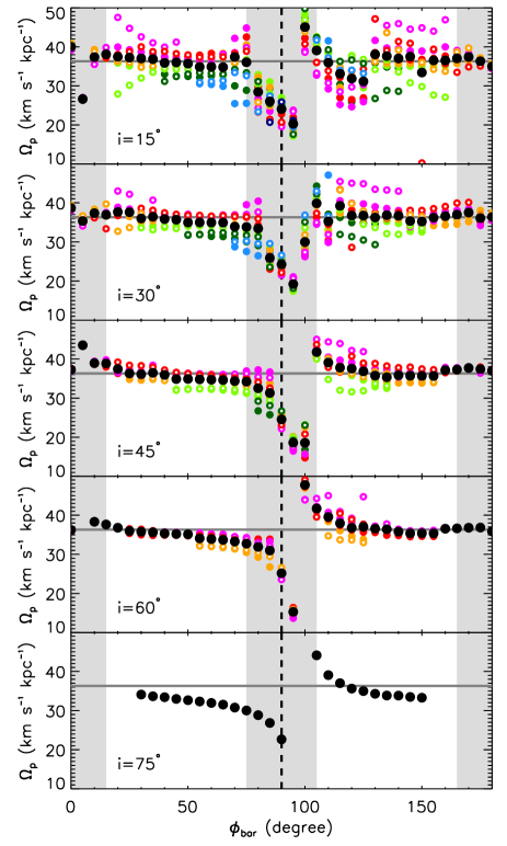
Figure 16: TW $\Omega_{\rm p}$ measurements for individual pseudo-slits (and their averages) as a function of $\phi_{\rm bar}$ and $i$. As in Figure 8, data points with different colors show pseudo-slits with different offsets from the simulated galaxy major axis (increasing from magenta to pale blue; see Fig. 4), with open and filled circles showing slits with the same offset but on the positive and negative side, respectively, of the major axis (see Fig. 4). The large black filled circles show the averages of all the slits. The thick gray solid horizontal lines show the intrinsic bar pattern speed of the simulated galaxy ($\Omega_{\rm p,int}=36.3$ km s^-1 kpc^-1), while the shaded gray areas show the bar angles when the bar is near the major or the minor axis of the disk. The bar pattern speeds $\Omega_{\rm p}$ are measured using the TW averaging method. The mock data sets used in this test have a $2\arcsec$ seeing, $1\farcs 2$ slit width, no binning, and $\delta$PA${}_{\rm disk}=0\arcdeg$.

Our tests therefore provide useful guidelines for the selection of observational samples for TW $\Omega_{\rm p}$ measurements. Indeed, using Figure 15, one can exclude inappropriate $\phi_{\rm bar}$ and $i$ that would result in significant measurement biases and/or uncertainties. For example, according to our simulation, and to keep both of these quantities to $\lesssim 10\%$, one should select barred disk galaxies with $10\arcdeg\lesssim\phi_{\rm bar}\lesssim 75\arcdeg$ and $105\arcdeg\lesssim\phi_{\rm bar}\lesssim 170\arcdeg$ and $15\arcdeg\lesssim i\lesssim 70\arcdeg$. Measurements are particularly inaccurate when the bar is close to the disk minor axis (see also Figure 16). It is worth noting that the optimal $\phi_{\rm bar}$ range is quoted in the intrinsic face-on values. In Figure 15, we also show the optimal observed $\phi_{\rm bar,obs}$ range with a black box when projection effects are taken into account (see Footnote 2). The optimal observed $\phi_{\rm bar,obs}$ range (black box) should be used when selecting samples for TW measurements.

Having said that, our tests are based on a single simulated barred galaxy, and the relative differences and uncertainties shown in Figure 15 would likely change slightly for other simulations/galaxies. In any case, as noted before, even favorable $(\phi_{\rm bar},i)$ pair TW $\Omega_{\rm p}$ measurements can still suffer from large biases because of other large-scale asymmetric structures such as spiral arms and lopsidedness. Our recommendation thus remains to always look at the $\Omega_{\rm p}$ distance profile for each slit and apply the convergence test discussed in § 4.1 and Figure 8.

4.7 Slit Width

Our mock data sets span pseudo-slit widths of $0\farcs 4$ to $2\arcsec$ in steps of $0\farcs 4$, with no overlap or gap between adjacent pseudo-slits. The number of slits that can be used thus decreases with increasing slit width (as the absolute size of the simulated galaxy is fixed). The bar pattern speeds measured from those individual pseudo-slits are shown in Figure 17, along with the averages using the TW averaging and TW fitting methods applied to the inner slits only.

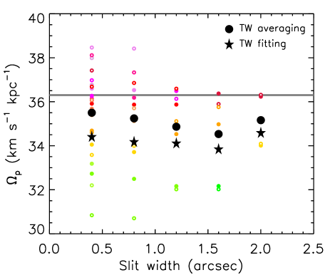
Figure 17: Slit width test. TW $\Omega_{\rm p}$ measurements are shown as a function of the width of the pseudo-slit used. Large black filled circles and stars show average measurements (inner slits only) using, respectively, the TW averaging and the TW fitting method. Small colored circles show $\Omega_{\rm p}$ measurements from individual pseudo-slits with different offsets from the major axis (see Fig. 4). The gray solid horizontal line shows the intrinsic $\Omega_{\rm p}$ of the simulated galaxy ($\Omega_{\rm p,int}=36.3$ km s^-1 kpc^-1). The mock data sets used in this test have $\phi_{\rm bar}=45\arcdeg$, $i=45\arcdeg$, $2\arcsec$ seeing, no binning, $\delta$PA${}_{\rm disk}=0\arcdeg$, and variable slit widths.

Overall, all the average measurements shown in Figure 17 are in agreement with each other to within $\approx 3\%$, well within any reasonable uncertainties (defined by, e.g., the scatter across individual measurements for each slit width). The slit width therefore has no significant effect on the measured average $\Omega_{\rm p}$.

As was already pointed out from Figure 12 (see also Fig. 9), we again note that the TW fitting method yields slightly and systematically lower measurements than the TW averaging method, but again this is only by a few percent and within reasonable uncertainties.

We also note that the scatter between individual measurements (i.e., the $\Omega_{\rm p}$ measured from individual slits) increases drastically for very narrow slits (i.e., slits significantly narrower than the seeing). As the measured $\Omega_{\rm p}$ varies systematically with the offset from the galaxy major axis (see § 4.2), this is probably simply due to the wider slits encompassing (and thus averaging) wider ranges of $\Omega_{\rm p}$. In any case, overly narrow pseudo-slits should be avoided for single slit measurements. Importantly, however, the average measurements remain reliable, so that again we conclude that the pseudo-slit width has no significant impact on the measurements.

4.8 Spatial Resolution

Angular resolution is usually considered very important for observations, as it determines the ability to see intricate spatial details in the objects studied. In optical/infrared observations, this angular resolution is usually quantified by the FWHM of the Gaussian PSF (i.e., the seeing). In this study, we use spatial and angular resolution interchangeably, as the distance to our simulated galaxy is fixed, and we use our simulation to test the influence of spatial resolution on TW measurements.

Figure 18 shows TW $\Omega_{\rm p}$ measurements using mock data sets with seeings ranging from $0\arcsec$ to $5\arcsec$ in steps of $0\farcs 5$, and using both the TW averaging and the TW fitting method. The average measurements using the TW fitting method are again slightly lower than those using the TW averaging method. Of more interest here, however, there is a weak trend of decreasing $\Omega_{\rm p}$ with increasing seeing for the innermost slits (i.e., the magenta, red, and orange datapoints in Fig. 18). The same trend is seen with other mock data sets with different $\phi_{\rm bar}$ and $i$, and it is easily understood from the trend of decreasing $\Omega_{\rm p}$ with increasing offset from the galaxy major axis described in § 4.2. Indeed, with increasingly bad seeing, particles at increasingly large $Y_{\rm grid}$ (or, equivalently, increasingly large major axis offsets) influence the observed surface brightnesses and velocities within any given pseudo-slit (see Eqs. 4 and 5). The measured $\Omega_{\rm p}$ thus decreases slightly but systematically with seeing. The opposite is true for the last inner slits near the ends of the bar (i.e., the green datapoints in Fig. 18), presumably for the same reason, i.e., with increasingly bad seeing particles at increasingly small $Y_{\rm grid}$ contribute to the measurements, and in consequence $\Omega_{\rm p}$ systematically increases with increasing seeing.

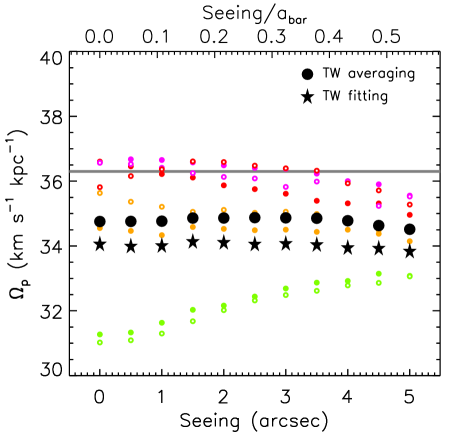
Figure 18: Spatial resolution test. TW $\Omega_{\rm p}$ measurements are shown as a function of the spatial resolution (seeing FWHM) used. Symbols and lines are as in Figure 17. The mock data sets used in this test have $\phi_{\rm bar}=45\arcdeg$, $i=45\arcdeg$, a $1\farcs 2$ slit width, no binning, $\delta$PA${}_{\rm disk}=0\arcdeg$, and variable seeing.

Most important here, however, is that the average measurements are essentially independent of seeing. Indeed, even for an unrealistically large seeing of $5\arcsec$, the relative error ($\Omega_{\rm p,5^{\prime\prime}}-\Omega_{\rm p,0^{\prime\prime}}$)/$\Omega_{\rm p,int}$ of the average measurements is $<1\%$, where $\Omega_{\rm p,5^{\prime\prime}}$ and $\Omega_{\rm p,0^{\prime\prime}}$ are the measured bar pattern speeds for respectively $5\arcsec$ and $0\arcsec$ seeing, respectively, and $\Omega_{\rm p,int}=36.3$ km s^-1 kpc^-1 is the known intrinsic bar pattern speed of the simulation. For a typical MaNGA seeing of $\approx 2\arcsec$, this relative error is also $<1\%$. Considering realistic uncertainties (again, e.g., the scatter across individual measurements for each seeing), Figure 18 suggests that spatial resolution has no significant effect on TW measurements. The TW method is thus reliable even at low spatial resolutions, as originally suggested by Tremaine & Weinberg (1984). Interestingly, it is thus well suited for poor-seeing backup observing programs.

4.9 TW Method and IFS Data

Combining the advantages of imaging and spectroscopy, IFSs are now available on most telescopes. These instruments, however, have different characteristics (wavelength coverage, FOV, spectral resolution, angular sampling, etc.), that make them most appropriate for different observational strategies and thus scientific goals. More IFSs will also come online in the near future.

For TW $\Omega_{\rm p}$ measurements, only those IFSs with a relatively large FOV are appropriate (see § 4.1). We therefore select some IFSs with a large FOV and summarize their characteristics in Table 1. All operate in the optical domain, with FOV diameters larger than $30\arcsec$ and spectral resolutions and angular samplings appropriate for dynamical work on nearby galaxies. Two Fabry-Perot instruments (GHaFaS and FaNTOmM) specifically target H$\alpha$ emission, thus providing high-quality spectra for application of the TW method to ionized gas. Their FOVs are very large, and spectral resolutions very high. A new generation of imaging Fourier transform spectrographs has similar strengths (SpIOMM and SITELLE). Instruments mounted on large telescopes and/or exploiting adaptive optics have particularly high angular samplings (MUSE, VIMOS, Kyoto3DII). Although a high spatial resolution is not crucial for TW measurements (see § 4.8), the data from these instruments also generally have higher S/N and can be binned more flexibly, which should lead to higher-quality TW $\Omega_{\rm p}$ measurements. The SparsePak, DensePak, and PPack family of fiber-fed IFSs have unusually high spectral resolutions, but this is unlikely to be a main driver for TW measurements.

Table 1: Characteristics of IFS instruments appropriate for TW pattern speed measurements.

Instrument	Wavelength Range	Spectral Res.	Spatial Sampling	Field of View	Telescope
	(Å)
RSS	$4300$ – $\phantom{,1}8600$	$300$ – $9000$	$0\farcs 13$	$8^{\prime}$	SALT 10 m
Kyoto3DII	$4000$ – $\phantom{,1}7000$	$400$, $7000$	$0\farcs 056$	$1\farcm 9\times 1\farcm 9$	Subaru 8.2 m
MUSE	$4650$ – $\phantom{,1}9300$	$\approx 3000$	$0\farcs 2$	$1^{\prime}\times 1^{\prime}$	VLT 8 m
VIMOS	$3600$ – $10,000$	$200$ – $2500$	$0\farcs 67$	$54\arcsec\times 54\arcsec$	VLT 8 m
SAURON	$4500$ – $\phantom{,1}7000$	$\approx 1500$	$0\farcs 94$	$41\arcsec\times 33\arcsec$	WHT 4.2 m
GHaFaS	$4500$ – $\phantom{,1}8500$	$\approx 20,000$	$0\farcs 4$	$3\farcm 4\times 3\farcm 4$	WHT 4.2 m
WEAVE∗	$3700$ – $\phantom{,1}9600$	$5000$, $20,000$	$1\farcs 3$, $2\farcs 6$	$11\arcsec\times 12\arcsec$, $78\arcsec\times 90\arcsec$	WHT 4.2 m
SAMI	$3700$ – $\phantom{,1}9500$	$1700$ – $13,000$	$1\farcs 6$	$15\arcsec$	AAT 3.9 m
DensePak	$3700$ – $11,000$	$5000$ – $20,000$	$3\farcs 0$	$30\arcsec\times 45\arcsec$	WIYN 3.8 m
SparsePak	$5000$ – $\phantom{,1}9000$	$5000$ – $20,000$	$4\farcs 7$	$72\arcsec\times 71\farcs 3$	WIYN 3.8 m
SITELLE	$3500$ – $\phantom{,1}9000$	$1$ – $10,000$	$0\farcs 32$	$11^{\prime}\times 11^{\prime}$	CFHT 3.6 m
PPak	$4000$ – $\phantom{,1}9000$	$\approx 8000$	$2\farcs 7$	$74\arcsec\times 64\arcsec$	Calar Alto 3.5 m
VIRUS-P	$3500$ – $\phantom{,1}6800$	$\approx 850$	$4\farcs 3$	$1\farcm 7\times 1\farcm 7$	McDonald 2.7 m
VIRUS-W	$4340$ – $\phantom{,1}6040$	$2500$, $6800$	$3\farcs 2$	$105\arcsec\times 75\arcsec$	McDonald 2.7 m
MaNGA	$3600$ – $10,400$	$\approx 2000$	$2\farcs 0$	$12\farcs 5$ – $32\farcs 5$	APO 2.5 m
CHILI∗	$3600$ – $\phantom{,1}7200$	$900$, $1900$	$5\farcs 6$	$71\arcsec\times 65\arcsec$	Lijiang 2.4 m
FaNTOmM	$4000$ – $\phantom{,1}9000$	$10,000$ – $60,000$	$1\farcs 6$	$17^{\prime}$	OMM 1.6 m
SpIOMM	$3500$ – $\phantom{,1}9000$	$1$ – $25,000$	$0\farcs 5$	$12^{\prime}\times 12^{\prime}$	OMM 1.6 m

Over the past two decades, the development of IFSs has motivated many IFS surveys of nearby galaxies, the most important of which are summarized in Table 2. The Spectral Areal Unit for Research on Optical Nebulae (SAURON) and subsequent Atlas^3D projects using the SAURON IFS pioneered large-scale surveys, observing a mass- ($K$-band luminosity) and volume-limited sample of $260$ early-type galaxies (Cappellari et al., 2011). The Calar Alto Legacy Integral Field Area (CALIFA) survey used the PPak IFS to study a sample of $\approx 670$ galaxies selected for their optical size (Sánchez et al., 2012). The VIRUS-P Exploration of Nearby Galaxies (VENGA) survey observed a sample of $30$ nearby spiral galaxies chosen for their extensive ancillary multiwavelength data (Blanc et al., 2013). The Sydney-Australian-Astronomical-Observatory Multi-object Integral-field Spectrograph (SAMI) survey is currently targeting $3400$ galaxies using a multiplexed fiber-fed IFS with two wavelength channels (Croom et al., 2012). The Mapping Nearby Galaxies at APO (MaNGA) project aims to observe $10,000$ galaxies over a wide range of stellar masses and environments (Bundy et al., 2015).

Table 2 shows that Atlas^3D has the best spatial sampling but a relatively small spatial coverage and poor velocity resolution. CALIFA has the largest FOV, helping to ensure that the optical extent of most galaxies is fully covered (and thus that the TW integrals converge). The FOV of VENGA is also large, but its velocity resolution is rather poor for TW measurements. SAMI and MaNGA have good compromises between FOV and spatial sampling, as well as between wavelength coverage and velocity resolution. The advantage of MaNGA is its large sample size, but SAMI covers a wider range of environments. Both should enable comprehensive studies of the correlations between bar pattern speeds and other properties of galaxies. The FOV of MaNGA reaches at least $1.5R_{\rm e}$ for two-thirds of the sample and at least $2.5R_{\rm e}$ for one-third, the latter being particularly promising given the convergence test discussed in § 4.1 (showing that TW $\Omega_{\rm p}$ measurements typically converge by $\approx 1.3R_{\rm e}$). As a second-generation IFS, the Multi Unit Spectroscopic Explorer (MUSE; Bacon et al., 2010) provides a unique combination of large FOV, high spatial sampling, and generally high S/N, offering new opportunities for accurate $\Omega_{\rm p}$ measurements using the TW method.

Table 2: Characteristics of relevant IFS surveys.

Survey	Sample Size	Field of View	Spatial Elements	Wavelength Range	Velocity Res.	Angular Res.
				(Å)	($\sigma$; km s-1)	(Reconstructed FWHM)
MaNGA	$10,000$	$>1.5$, $>2.5$ $R_{\rm e}$	$19$ – $127$	$3600$ – $10,300$	$50$ – $80$	$\approx 2\farcs 5$
WEAVE	$5000$	$11\arcsec\times 12\arcsec$, $78\arcsec\times 90\arcsec$	$37$, $540$	$3660$ – $\phantom{,1}9840$	$15$, $60$	$\cdots$
SAMI	$3400$	$>1$ $R_{\rm e}$	$61$	$3700$ – $\phantom{,1}5700$	$70$	$\approx 2\farcs 2$
				$6300$ – $\phantom{,1}7400$	$30$	$\approx 2\farcs 2$
CALIFA	$667$	$>2.5$ $R_{\rm e}$	$331$	$3700$ – $\phantom{,1}7000$	$85$, $150$	$\approx 2\farcs 4$
Atlas3D	$260$	$\approx 1$ $R_{\rm e}$	$1431$	$4800$ – $\phantom{,1}5380$	$105$	$\cdots$
SIGNALS	$38$	$11\arcmin\times 11\arcmin$	$\approx 4,500,000$	$3630$ – $\phantom{,1}6850$	$60$	$\approx 0\farcs 8$
VENGA	$30$	$\approx 0.7$ $R_{\rm 25}$∗	$246$	$3600$ – $\phantom{,1}6800$	$\approx 120$	$\approx 5\farcs 6$

5 Conclusions

In this work, we aimed to assess the potential limitations, biases, and uncertainties of direct bar pattern speed ($\Omega_{\rm p}$) measurements using the method proposed by Tremaine & Weinberg (1984), with a special emphasis on IFS observations. To achieve this, we used a simple $N$-body simulation of a barred disk galaxy and created a series of mock data sets with different alignments of the galaxy major axis with respect to the data/grid axes (PA_disk), bar angles with respect to the galaxy major axis ($\phi_{\rm bar}$), disk inclinations ($i$), (pseudo-)slit widths, spatial resolutions (seeings), spatial binnings, and position angle misalignments. We summarize our main findings below.

(i) A convergence test is essential to establish the reliability of any TW $\Omega_{\rm p}$ measurement, whereby a profile of the derived $\Omega_{\rm p}$ is constructed as a function of the distance along the slit (i.e., the integration limits of the TW integrals). This profile should converge to a constant value for any measurement to be deemed reliable, and it therefore determines the minimum field of view (or, equivalently, the minimum [half-]slit length) required for accurate measurements (a projected distance of $1.3$ times the effective or half-mass radius for our simulation).

(ii) We find that the derived $\Omega_{\rm p}$ is increasingly biased low as the offset of a (pseudo-)slit from the galaxy major axis increases, and that only (pseudo-)slits located within the bar region yield accurate measurements.

Bar pattern speeds measured from slits beyond the bar can be significantly affected by other large-scale asymmetric structures with different (generally lower) pattern speeds, such as spiral arms and lopsidedness. In consequence, when slits near the ends of the bar are used, the TW fitting method generally yields slightly lower TW $\Omega_{\rm p}$ measurements than the TW averaging method.

(iii) Bar pattern speed measurements using IFSs are not significantly affected by spatial binning unless the bins are extremely large and/or few, when TW $\Omega_{\rm p}$ measurements can be underestimated by as much as $\approx 15\%$. IFS data with a number of bins smaller than $\approx 200$ in an FOV of $20\times 20$ kpc² should not be used for TW measurements.

(iv) We find no significant dependence of the TW $\Omega_{\rm p}$ measurements on the position angle of the disk within the IFS FOV. However, recasting the grid to align the disk major axis with the data/grid axes does lead to smaller uncertainties on the measurements (compared to naive integrations along irregularly shaped slits comprising only those spaxels whose center falls within the desired perfectly rectangular slits).

(v) We confirm the finding of D03 that the TW method is very sensitive to misalignments of the disk position angle (and thus the orientation of the pseudo-slits). Position angle misalignments lead to TW $\Omega_{\rm p}$ measurement errors that are both the largest and are systematic. For a misalignment of as little as $5\arcdeg$, the relative $\Omega_{\rm p}$ systematic error can be as large as $35\%$. When the angle between the bar and the assumed disk major axis is wrongly increased, the inferred $\Omega_{\rm p}$ can be severely overestimated, leading, for example, to apparently ultrafast bars, conversely when the angle between the bar and the assumed disk major axis is wrongly decreased. We unfortunately fail to build a sufficiently accurate empirical disk position angle diagnostic, but we do provide approximate diagnostics pointing the way for future studies.

(vi) Given the limitations introduced by both observational effects and the TW formalism itself, we determined the optimal $\phi_{\rm bar}$ and $i$ ranges for accurate TW $\Omega_{\rm p}$ measurements. For our simulation, the relative biases and uncertainties can be kept to $\lesssim 10\%$ for $10\arcdeg\lesssim\phi_{\rm bar}\lesssim 75\arcdeg$ and $105\arcdeg\lesssim\phi_{\rm bar}\lesssim 170\arcdeg$ and $15\arcdeg\lesssim i\lesssim 70\arcdeg$. Measured bar pattern speeds are significantly less accurate when the bar is close to the disk minor axis.

(vii) We find that unless the slit width is significantly smaller than the seeing, the slit width does not affect TW $\Omega_{\rm p}$ measurements significantly.

(viii) As expected from the TW formalism, the spatial resolution (i.e., seeing) of the observations does not have a significant impact on TW $\Omega_{\rm p}$ measurements either.

To improve current TW bar pattern speed measurements, we thus suggest to choose targets with appropriate viewing angles ($\phi_{\rm bar}$ and $i$), to select the pseudo-slits carefully, and to apply the convergence test for every slit in every galaxy. Most importantly, only those galaxies with small major axis position angle uncertainties should be considered. Minor improvements can be obtained by paying attention to the grid recasting.

Our results suggest that it is possible to wrongfully infer ultrafast bars if the angle between the bar and the assumed disk major axis is overestimated, if the bar is close to the disk minor axis, and/or if the FOV is too small for convergence.

Our tests thus provide useful guidelines for future applications of the TW method to real data, particularly IFS observations. However, as our tests are based on a single simulation, the exact limitations, biases, and uncertainties of TW $\Omega_{\rm p}$ measurements will vary slightly from galaxy to galaxy.

References

- Aguerri et al. (1998) Aguerri, J. A. L., Beckman, J. E., & Prieto, M. 1998, AJ, 116, 2136
- Aguerri et al. (2003) Aguerri, J. A. L., Debattista, V. P., & Corsini, E. M. 2003, MNRAS, 338, 465
- Aguerri et al. (2009) Aguerri, J. A. L., Méndez-Abreu, J., & Corsini, E. M. 2009, A&A, 495, 491
- Aguerri et al. (2000) Aguerri, J. A. L., Muñoz-Tuñón, C., Varela, A. M., & Prieto, M. 2000, A&A, 361, 841
- Aguerri et al. (2015) Aguerri, J. A. L., Méndez-Abreu, J., Falcón-Barroso, J., et al. 2015, A&A, 576, A102
- Athanassoula (1992a) Athanassoula, E. 1992a, MNRAS, 259, 328
- Athanassoula (1992b) —. 1992b, MNRAS, 259, 345
- Athanassoula (2003) —. 2003, MNRAS, 341, 1179
- Bacon et al. (2010) Bacon, R., Accardo, M., Adjali, L., et al. 2010, in Society of Photo-Optical Instrumentation Engineers (SPIE) Conference Series, Vol. 7735, Ground-based and Airborne Instrumentation for Astronomy III, 773508
- Banerjee et al. (2013) Banerjee, A., Patra, N. N., Chengalur, J. N., & Begum, A. 2013, MNRAS, 434, 1257
- Barazza et al. (2008) Barazza, F. D., Jogee, S., & Marinova, I. 2008, ApJ, 675, 1194
- Beckman et al. (2018) Beckman, J. E., Font, J., Borlaff, A., & García-Lorenzo, B. 2018, ApJ, 854, 182
- Blanc et al. (2013) Blanc, G. A., Schruba, A., Evans, Neal J., I., et al. 2013, ApJ, 764, 117
- Bundy et al. (2015) Bundy, K., Bershady, M. A., Law, D. R., et al. 2015, ApJ, 798, 7
- Bureau et al. (1999) Bureau, M., Freeman, K. C., Pfitzner, D. W., & Meurer, G. R. 1999, AJ, 118, 2158
- Buta (1986) Buta, R. 1986, ApJS, 61, 609
- Buta et al. (1995) Buta, R., van Driel, W., Braine, J., et al. 1995, ApJ, 450, 593
- Buta & Zhang (2009) Buta, R. J., & Zhang, X. 2009, ApJS, 182, 559
- Canzian (1993) Canzian, B. 1993, ApJ, 414, 487
- Canzian & Allen (1997) Canzian, B., & Allen, R. J. 1997, ApJ, 479, 723
- Cappellari & Copin (2003) Cappellari, M., & Copin, Y. 2003, MNRAS, 342, 345
- Cappellari et al. (2011) Cappellari, M., Emsellem, E., Krajnović, D., et al. 2011, MNRAS, 413, 813
- Cepa & Beckman (1990) Cepa, J., & Beckman, J. E. 1990, A&A, 239, 85
- Chemin & Hernandez (2009) Chemin, L., & Hernandez, O. 2009, A&A, 499, L25
- Contopoulos (1980) Contopoulos, G. 1980, A&A, 81, 198
- Corsini et al. (2007) Corsini, E. M., Aguerri, J. A. L., Debattista, V. P., et al. 2007, ApJ, 659, L121
- Corsini et al. (2003) Corsini, E. M., Debattista, V. P., & Aguerri, J. A. L. 2003, ApJ, 599, L29
- Croom et al. (2012) Croom, S. M., Lawrence, J. S., Bland-Hawthorn, J., et al. 2012, MNRAS, 421, 872
- Debattista (2003) Debattista, V. P. 2003, MNRAS, 342, 1194, (D03)
- Debattista et al. (2002) Debattista, V. P., Corsini, E. M., & Aguerri, J. A. L. 2002, MNRAS, 332, 65
- Debattista & Sellwood (1998) Debattista, V. P., & Sellwood, J. A. 1998, ApJ, 493, L5
- Debattista & Sellwood (2000) —. 2000, ApJ, 543, 704
- Debattista & Williams (2004) Debattista, V. P., & Williams, T. B. 2004, ApJ, 605, 714
- Emsellem et al. (2006) Emsellem, E., Fathi, K., Wozniak, H., et al. 2006, MNRAS, 365, 367
- Eskridge et al. (2000) Eskridge, P. B., Frogel, J. A., Pogge, R. W., et al. 2000, AJ, 119, 536
- Fathi et al. (2009) Fathi, K., Beckman, J. E., Piñol-Ferrer, N., et al. 2009, ApJ, 704, 1657
- Fathi et al. (2007) Fathi, K., Toonen, S., Falcón-Barroso, J., et al. 2007, ApJ, 667, L137
- Font et al. (2011) Font, J., Beckman, J. E., Epinat, B., et al. 2011, ApJ, 741, L14
- Font et al. (2014) Font, J., Beckman, J. E., Querejeta, M., et al. 2014, ApJS, 210, 2
- Fragkoudi et al. (2017) Fragkoudi, F., Athanassoula, E., & Bosma, A. 2017, MNRAS, 466, 474
- Gabbasov et al. (2009) Gabbasov, R. F., Repetto, P., & Rosado, M. 2009, ApJ, 702, 392
- Gerssen et al. (1999) Gerssen, J., Kuijken, K., & Merrifield, M. R. 1999, MNRAS, 306, 926
- Gerssen et al. (2003) —. 2003, MNRAS, 345, 261
- Gunn et al. (2006) Gunn, J. E., Siegmund, W. A., Mannery, E. J., et al. 2006, AJ, 131, 2332
- Guo et al. (2019) Guo, R., Mao, S., Athanassoula, E., et al. 2019, MNRAS, 482, 1733
- Hernandez et al. (2005) Hernandez, O., Wozniak, H., Carignan, C., et al. 2005, ApJ, 632, 253
- Kent (1987) Kent, S. M. 1987, AJ, 93, 1062
- Marinova & Jogee (2007) Marinova, I., & Jogee, S. 2007, ApJ, 659, 1176
- Menéndez-Delmestre et al. (2007) Menéndez-Delmestre, K., Sheth, K., Schinnerer, E., Jarrett, T. H., & Scoville, N. Z. 2007, ApJ, 657, 790