Quantum Creation of a Toy Universe without Inflation
Abstract
We propose a toy model for the origin of the universe, where the scale-invariant fluctuations are generated together with the quantum creation process of the universe. The fluctuations arise inside an instanton in the Euclidean domain of time. In the Lorentzian point of view, the universe emerges with passive, coherent and scale-invariant fluctuations present from the beginning, without the need of inflation or a bounce. For this mechanism to work, we need anisotropic scaling in space and time, which is realized in a toy model of Horava-Lifshitz gravity with a Lifshitz scalar field.
1 Introduction
Inflation [1, 2, 3, 4, 5, 6] is currently the leading paradigm of the very early universe cosmology. The existence of an inflationary period reduces the spatial curvature and increases the particle horizon, which solve the flatness problem and the horizon problem. Most importantly, the inflationary paradigm provides a predictive theory of the primordial cosmological perturbations [7, 8, 9, 10, 11, 12, 13], generating a near scale-invariant power spectrum, as later observed by cosmological experiments [14, 15, 16].
Despite its success, there are many open questions (sometimes considered as problems) for inflationary cosmology, see [17, 18, 19] for reviews. The inflationary spacetime is past-incomplete [20], and may have an initial singularity [21]. This suggests that inflation cannot provide a complete description of the very early universe. Another issue is the trans-Planckian problem for cosmological fluctuations [22]. The inflationary fluctuations may potentially begin in a super-Planckian region where currently known physical laws may be invalid. A further issue is that, for inflation to happen, the pre-inflationary universe is restricted to be somewhat old, large and homogeneous [23, 24], introducing new initial condition problems. In some inflation models, e.g. the chaotic inflation [23] and eternal inflation [25], this prerequisite can be generic, but a measure problem arises relating to whether we are typical observers [26, 27, 28]. Also, models of inflationary cosmology relying on scalar fields need to satisfy stringent constraints, which constitutes another initial condition problem for inflation [29].
These open questions do not imply a failure of the inflationary paradigm. In fact, many possible solutions have been proposed within the inflationary paradigm for each of the problems here. However, we need to look out of the paradigm of inflation, to judge whether these solutions are economical or artificial. Thus, to measure the success of inflation, it is important to explore possible alternative scenarios to inflation. And these alternative theories may have a chance to succeed in their own rights.
Generally, an alternative to inflation scenario is expected to generate near scale-invariant fluctuations, as these fluctuations are already observed. Usually, this automatically solves the horizon problem. At best, the scenario should also solve the flatness problem and possibly other problems that inflation encounters.
There have been many alternative to inflation scenarios in the literature. To the best of our knowledge, all of these alternatives can be classified by the time-dependence of the scale factor where the time variable is real. Some examples, sorted not by physical realization but by the scale factor behavior in real time, include fast contraction [30, 31], slow contraction [32], slow expansion [33, 34, 35, 36] and fast non-exponential expansion [37]. For a review of alternative scenarios to inflation, see [17].
In this paper, we propose a different approach. The scale-invariant fluctuations are generated inside an instaton, where the time variable is complex. In the Lorentzian point of view, the universe emerges quantum mechanically with all the fluctuations already present at the emergence of the universe.
To describe the quantum creation of the universe, we presume the formalism of Euclidean quantum gravity (EQG) with the no boundary initial condition [38, 39, 40, 41, 42, 43] (see also [44, 45] for a different approach). In this formalism, the universe is created “from nothing” (i.e. from a state with scale factor ) quantum mechanically. The relative probability amplitude of the quantum creation is determined by a Euclidean path integral. In the minimal setup, the quantum created universe in EQG is curvature dominated or empty [46]. And the quantum fluctuations are in their Bunch-Davies vacuum states after the quantum creation [40]. Such universes cannot be considered as alternatives to inflation since they are not suitable in size, and have no scale-invariant fluctuations in it.
Recently, [47] proposed that in Horava-Lifshitz (HL) gravity [48], the universe starts its cosmological evolution in a relatively flat configuration and the flatness problem is resolved. A large universe can be quantum created if suitable model parameters are chosen. In this paper, we will use the background model in [47] to create a large and flat universe. After discussing the flatness problem in detail, we work out the scalar perturbation and show that the near scale-invariant power spectrum can be obtained from a Lifshitz scalar field.
The paper is organized as follows. In section 2 we introduce our model. Then in section 3 we analyze the dynamics of cosmological background as well as the flatness problem. After that, we study the scalar perturbation and discuss how the observed near scale-invariant power spectrum can be obtained in section 4. A numerical study is then given in section 5 to verify some approximations in previous sections. Finally, we conclude in section 6 and discuss some future directions.
2 A Concrete Model
2.1 The Metric and the Action
We decompose the metric using the ADM formalism [49]:
| (2.1) |
Here is the time coordinate, (=1, 2, 3) are spatial coordinates. The constraints and dynamics in the metric are encoded in the lapse function , shift vector and the 3-metric .
We consider the projectable version of HL gravity (see appendix B for a brief introduction). In 4 spacetime dimensions, the most general action for HL theory minimally coupled with a scalar field is
| (2.2) |
where and are restricted by the HL symmetry and their most general forms are
| (2.3) |
where
| (2.4) |
The matter action takes the form [50]
| (2.5) |
2.2 Cosmological Evolution Indicated by EQG Formalism
In EQG formalism, the universe starts in the quantum gravity (QG) region (or called the Euclidean region since the time is imaginary), during which the state of the universe is described by its wave function , defined as the path integral over possible compact configurations with boundary geometry and matter be and :
| (2.6) |
where and are the three-geometry and matter field configuration at the end of the state, and is the Euclidean action obtained from (2.2) by a Wick rotation of time . Hawking’s no boundary proposal [51] is applied, so the path integral (2.6) is defined over all possible paths which start from a vanishing universe, go through compact configurations and end in the final configuration .
The relative probability for the universe to be in a certain configuration is . We assume that the dynamics of the universe is described by the most probable path, that is, the path that follows the classical equation of motion (EoM) with background geometry to be the Friedmann-Robertson-Walker (FRW) metric [52].
The universe will end its QG evolution and tunnel to Lorentzian spacetime, and the time becomes real. After the quantum tunneling, the evolution of the universe is predicted by standard cosmology. An inverse Wick rotation is presented: where represents the Lorentzian time at the quantum tunneling event.
2.3 Spectator Field Approximation
For simplicity, we use spectator field approximation throughout this work. By “spectator”, gravity is just a background and does not receive back-reaction from the scalar field. The field fluctuation may convert to curvature perturbation through a rolling background, or the curvaton mechanism [53, 54] or the modulated reheating [55, 56, 57].
The spectator field approximation allows us to separate the gravity action and matter action . The wave function of universe (2.6) can be decomposed into
| (2.7) |
The gravity part uniquely determines the dynamics of the background. Under the spectator field approximation, there is no metric perturbation, so the scalar perturbation is uniquely determined by .
3 The Background Cosmology
3.1 Classical Background EoM
We consider a homogeneous and isotropic closed universe, the metric is:
| (3.1) |
Here is the metric of a unit sphere, so the scale factor represents the radius of the universe and has the dimension of length.
3.2 Background Dynamics in the Euclidean Region
In the Euclidean region, the time is imaginary. We make a Wick rotation , and define . Also for convenience, we define . In the IR region, our model should recover standard GR in which due to higher symmetry. Since there exists an IR Gaussian fixed point where and [59], we may reasonably take and . The EoM (3.3) is then:
| (3.4) |
Here is dimensionless, has dimension or , and has dimension . So the model parameter and should have dimension and , respectively.
3.3 Initial Condition and Final State of Euclidean Evolution
In EQG, the universe starts with a vanishing size in the Euclidean regime. In later calculations, we need the asymptotic behavior of near . Expanding in the neighbor of and keeping the two leading terms, we have
| (3.5) |
Substituting (3.5) into (3.4) and equating the two highest power of gives
| (3.6) |
At the end of the Euclidean evolution, the universe tunnels to Lorentzian spacetime, and the time becomes real. Labeling the tunneling time as , the condition that quantum tunneling happens is , or equivalently .
Define , the tunneling condition along with (3.4) gives: . To generate a flat enough universe, the curvature component at the moment of tunneling should be subdominant compared to other terms: . This gives an approximated value .
3.4 The Flatness of the Universe
The conditions required to create a universe flat enough to be consistent with observations is that the model should predict a subdominant curvature component at the very beginning of the Lorentzian region. If this was true, at we have and
| (3.7) |
Since is a non-zero quantity, (3.7) implies that a large , or equivalently, a strong presence of dark matter is needed for generating a flat enough universe.
Physically, the HL coupling dominates at first for its dependence. As the scale factor increases, the curvature term becomes more and more important, so a relatively large can help to end the Euclidean evolution quickly to avoid the domination of the curvature component. Thus, the flatness problem is turned into a fine-tuning problem between the model parameter and an integration constant111This fine-tuning problem is not a technical naturalness problem since is an integration constant, similar to the situation of unimodular gravity with the cosmological constant problem [60]..
4 Analysis of Perturbations
4.1 Quadratic Action of Perturbations
Recall that, the perturbations come solely from the scalar field under the spectator field approximation, of which the most general action is (2.5); if we substitute , and to its background value , 1 and , and take only terms for simplicity, the action becomes:
| (4.1) |
We separate the matter field as a homogeneous and isotropic background and perturbation , which can be expanded as a summation of spherical harmonics:
| (4.2) |
where is defined as the normalized eigenfunction of the Laplacian operator on three-dimensional unit sphere : and . We have suppressed the other two indices since they are irrelevant to our work. Inserting (4.2) into (4.1), the quadratic action for perturbation modes is:
| (4.3) |
where a dot denotes differentiation with respect to time, and is defined by
| (4.4) |
The approximation comes from the fact that the wavelengths of currently observed perturbations are much larger than . Also, we can obtain the Euclidean action for perturbation by a Wick rotation :
| (4.5) |
where a prime denotes differentiation with respect to .
From (4.5), perturbations of different wavenumbers are separable, which enables us to define the action for a single wavenumber of perturbation:
| (4.6) |
4.2 Classical EoM and Initial Asymptotic Behavior of Perturbations
The classical EoM for comes from the variation of (4.6) with respect to :
| (4.7) |
For later convenience, we shall introduce . Then (4.7) becomes
| (4.8) |
The asymptotic behavior of around can uniquely determine the asymptotic behavior of perturbations. Recall that near , this gives , and (4.7) becomes
| (4.9) |
(4.9) has the form of a Bessel equation, and its general solution is
| (4.10) |
where and are the Bessel and Neumann functions. Note that is divergent near , so should be set to 0 for a finite perturbation. Furthermore, as we shall see later, the magnitude of is irrelevant to our work, so we can safely take and the only possible asymptotic form of is
| (4.11) |
The asymptotic behavior of around is
| (4.12) |
4.3 The Wave Function of Perturbation Modes
The decomposition of perturbations with different wavenumbers enables us to define the wave function for :
| (4.13) |
The path integral (4.13) can be evaluated by the WKB approximation, which states that the dominating contribution of the path integral comes from the neighbor of classical trajectory. Following the method in [40], we use integration by parts to transform (4.6) to
| (4.14) |
where is the operator satisfying the classical equation of motion , which originates from the variation of (4.6) with respect to . Explicitly we have
| (4.15) |
and is the induced boundary term
| (4.16) |
Under the WKB approximation, does not contribute to the correlation function. The main contribution to the two-point correlation function comes from the quadratic term of :
| (4.17) |
and the wave function is rewritten as
| (4.18) |
4.4 Two-Point Correlation Function and Power Spectrum
The two-point correlation function of at can be evaluated as
| (4.19) |
Note that, (4.19) is independent on the overall magnitude of , which justifies the specific choice of in (4.11). Besides, (4.19) implicitly contains a delta function due to the decomposition of different wavenumbers.
(4.19) is implicitly related to the model parameters by the classical EoM of (4.8). As we will show numerically in section 5, the solution to (4.8) near the tunneling event can be approximated as . We may understand this fact by the observation that, the term is subdominant close to from the tunneling condition , and the remaining equation has a general solution , which approximates to at large enough . (4.19) can then be explicitly expressed by the model parameters:
| (4.20) |
Now we see that the dependence of the two-point correlation function comes solely from , since and are constants. Comparing with the definition of the power spectrum
| (4.21) |
we have
| (4.22) |
To generate a near scale-invariant power spectrum (i.e. ), we need . From (4.4) we see this can be accomplished as long as the positive term dominates the expression.
4.5 Spectral Index
Although the scalar perturbations are nearly scale invariant, a small tilt is observed. The spectral index as is observationally constrained by [16]. The standard cosmology connects observed cosmological fluctuations today with those at very early times by the adiabatic modes which is conserved outside the horizon [61]. In inflationary cosmology, the related perturbation modes will all exit the horizon during the quasi de-Sitter period.
In our model, however, the scalar perturbation is inside the horizon at because of the tunneling condition , so the two-point function also depends on the physics after the tunneling. We analyze two cases and see how a slight tilt is generated.
If a quick reheating process happens right after the quantum tunneling and turns the dark matter and HL coupling into radiation, then the time of horizon exiting is just the tunneling time , due to the finiteness of and largeness of .In this case, (4.20) is valid and the tilt generated by subdominated terms in (4.4) is
| (4.23) |
which had better be negative inspired by observations [16]. However, in the IR region, the standard dispersion relation suggests that and should be positive. So in this case, the condition for a power spectrum with red tilt is
| (4.24) |
If the reheating process is slow, the perturbation modes will exit the horizon when the dark matter and HL coupling still dominate, during which the dynamics of the universe is described by
| (4.25) |
Define the time for horizon exiting of mode as , the horizon exiting condition is , or , from which we can estimate
| (4.26) |
here the condition (3.7) is applied. Now the two-point correlation function of at horizon exiting is
| (4.27) |
We can see that the term in and the term square brackets combined produce a dependence in the two-point function. The red tilt can be generated from the term, so in this case (4.24) is no longer required.
Finally, recall that we need a rolling background, or curvaton, or modulated reheating to convert the spectator fluctuation into curvature fluctuation. In this conversion process, a further tilt may be generated and contribute to the final spectral index.
5 A Numerical Study
We present here a numerical case. To avoid the appearance of large numbers, we rescale the parameters: we set a length scale with dimension , and define
| (5.1) |
Now , , and are all dimensionless. The EoM (3.4) then becomes
| (5.2) |
We take , , and . The original model parameters are then , and . The tunneling condition gives the constraint on scaled scale factor at the tunneling time :
| (5.3) |
Numerically it gives . The real scale factor . Note that needs to be extremely large to be consistent with a currently flat universe. This statement is checked in Appendix D.
We check how (3.7) is satisfied in this numerical case. The ratio in our numerical case is small and close to the current proportion of gravity [15]. We then see that the flatness problem is transferred to a parameter choice problem in our model.
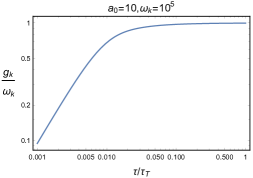
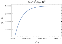
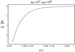
For perturbations, as mentioned in section 4, the observational effect of perturbation originates from , which is determined by (4.8). To show that the validity of our approximation in section 4 is generic and to avoid the possible numerical deviation from large numbers, we numerically calculated with different but relatively small . The result is presented in figure 1, we see that the asymptotical behavior of near the tunneling point supports (4.8).
6 Conclusion and Discussion
In this paper, we construct a toy model for alternative to inflation. The model is motivated by some current puzzles for inflationary cosmology. If we do not introduce scenarios like bouncing cosmology [62, 32, 63, 64, 65, 66, 67, 68, 69], the very early universe will undergo quantum gravity effects, especially in the initial singularity of Big Bang cosmology. In this case, we should include some theory of quantum gravity for a complete description of the very early universe. We choose the underlying theory to be Hawking’s EQG formalism, since it predicts the relative probabilities of any configuration of the universe, thus the fine-tuning problems from flatness problem and initial condition problem can be transferred into a matter of probability. We have seen in section 3 that, with properly chosen parameters, the most probable universe created by the HH instanton will have a large radius, which is consistent with the smallness of today. Also, the Euclidean action reaches its minimum when the universe is in the maximum symmetric configuration [70], in EQG this means an initially homogeneous universe is the most probable, which might be employed to explain the initial condition problem.
After that, we need the action of gravity and matter, as well as the boundary condition to determine the cosmological evolution. The boundary condition is chosen to be Hawking’s no boundary proposal since it can interpret the initial singularity [51]. The action should be renormalizable, otherwise, the theory cannot be applied to Planck scale, contradicting with our motivation for explaining the initial singularity of the universe, which provides us an additional motivation of choosing HL action. Now the model is constructed, and we have seen that the puzzles in inflationary cosmology may get explanations under our framework.
Once we construct the toy model, it is important to check whether it can reproduce the successful prediction in inflationary cosmology. The horizon problem is automatically solved since at all modes are casually connected. We verify that our model may transfer the flatness problem into a tuning problem of model parameters in section 3, and confirm that a near-scale invariant power spectrum may be generated from the Lifshitz field in section 4.
After setting up the framework of this Euclidean alternative to inflation approach in this paper, it is interesting to explore many further directions. For example,
- -
-
-
We have studied a spectator field. The spectator fluctuation can be converted to curvature by mechanisms such as curvaton [53, 54] or modulated reheating [55, 56, 57]. However, it is more interesting to study the possibility if the curvature perturbation is directly created in the EQG approach. Thus, it is interesting to calculate the full perturbation theory in EDG with gravitational fluctuations.
-
-
The existence of requires the violation of Hamiltonian constraints which is not observed yet; and the non-trivial geometry (see appendix C) is not observable. so it is interesting to seek for other mechanisms (for example, a HL action with different anisotropy scaling, or some renormalizable gravity action) to replace , avoiding the above requirements.
-
-
The parameter appears as an integration constant here. This constant may be explained as dark matter considering how its energy density evolves with time. However, it is important to find a mechanism to either realize a radiation dominated universe from the decay of this “dark matter” component or add more realistic matter into the model to take the role of starting a radiation dominated universe.
-
-
We have found that the feature of power spectrum can be produced by the Lifshitz field; and it’s natural to guess if the metric perturbation of HL gravity alone can give such a feature since both of them are characterized by the anisotropic scaling.
-
-
How to model-independently test this scenario against inflation and other alternative scenarios? Model-independent tests of primordial universe scenarios include the spectrum of primordial gravitational waves, and primordial quantum standard clocks [74, 75, 76]. It is interesting to see how these criteria work in the Euclidean time regime.
We hope to address these issues in further works.
Acknowledgments
We thank Yifu Cai, Andrew Cohen, Qianhang Ding, Xian Gao, Shinji Mukohyama, Xi Tong, Henry Tye and Siyi Zhou for the delightful discussion. This research was supported in part by GRF Grant 16304418 from the Research Grants Council of Hong Kong.
Appendix A Conventions
In this paper Planck units are used, in which . We keep the Planck length , time and energy reserved, but use and interchangeably. The scale factor is defined by the FRW metric with positive curvature:
| (A.1) |
Here is the metric of a unit sphere, so the scale factor represents the radius of the universe, which has length dimension.
Appendix B Preliminary Introduction to Projectable HL gravity
In this section, we will follow [77]. A basic property of HL gravity is the anisotropy scaling:
| (B.1) |
where is called the dynamical critical exponent. In 4 dimensional spacetime, anisotropic scaling of can make the gravity renormalizable in the UV region and can also lead to a scale-invariant cosmological perturbation [37]. In infrared(IR) region the theory should flow to to recover GR. So for our purpose, we concern on the HL action composed of and gravity sector, and the most general form of which is:
| (B.2) |
where
| (B.3) |
Here , is the extrinsic curvature, and are separately the covariant derivatives and the Ricci tensor of while is the intrinsic curvature. and (n=1,…,5) are constants.
The existence of anisotropic scaling breaks the Lorentz symmetry. Instead, the fundamental symmetry of the theory is are invariance under space-independent time reparametrization and time-dependent spatial diffeomorphism:
| (B.4) |
The symmetry, as well as the fact that only depends on , allows us to set by a time reparametrization .
The most general renormalizable action for a single scalar field compatible in dimension with the symmetry of HL theory is [50]
| (B.5) |
where is the Laplacian operator, is restricted by , and are constants. The represents all possible independent combinations of and up to a total derivative, for example:
| (B.6) |
For our case, and , (B.5) becomes
| (B.7) |
Appendix C Using Non-Trivial Geometries to Release the Constraint on
In canonical gravity theory, the total Hamiltonian of gravity is 0 due to the existence of a secondary constraint (the Hamiltonian constraint) [78, 79]:
| (C.1) |
(3.3), (C.1) combined give . To make the integration constant non-vanishing, the spatial geometry is assumed to have non-trivial topology, composed of several connected pieces, but each of which is disconnected with others[80]. The constraint then becomes a summation
| (C.2) |
Take our universe to be one of the connected pieces, the restriction of integration constant is now evaded.
Appendix D Estimation on Scale Factor at Quantum Tunneling
Here we estimate the parameter space of . Given today’s observation (here denotes the time today) [15]
| (D.1) |
we can estimate a lower limit of today’s radius of universe . We then use the redshift of matter-radiation domination epoch to get .
Now the energy scale at is . The energy scale at quantum tunneling should be larger than , the EW phase transition scale, but less than the Planck scale . We then have
| (D.2) |
In section 5, we choose parameters so that . The corresponding energy scale is , which is close to the GUT scale .
References
- [1] Alan H. Guth. The Inflationary Universe: A Possible Solution to the Horizon and Flatness Problems. Phys. Rev., D23:347–356, 1981. [Adv. Ser. Astrophys. Cosmol.3,139(1987)].
- [2] Andrei D. Linde. A New Inflationary Universe Scenario: A Possible Solution of the Horizon, Flatness, Homogeneity, Isotropy and Primordial Monopole Problems. Phys. Lett., 108B:389–393, 1982. [Adv. Ser. Astrophys. Cosmol.3,149(1987)].
- [3] Andreas Albrecht and Paul J. Steinhardt. Cosmology for Grand Unified Theories with Radiatively Induced Symmetry Breaking. Phys. Rev. Lett., 48:1220–1223, 1982. [Adv. Ser. Astrophys. Cosmol.3,158(1987)].
- [4] S. W. Hawking and I. G. Moss. Supercooled Phase Transitions in the Very Early Universe. Phys. Lett., 110B:35–38, 1982. [Adv. Ser. Astrophys. Cosmol.3,154(1987)].
- [5] L. Z. Fang. Entropy Generation in the Early Universe by Dissipative Processes Near the Higgs’ Phase Transitions. Phys. Lett., 95B:154–156, 1980.
- [6] Alexei A. Starobinsky. A New Type of Isotropic Cosmological Models Without Singularity. Phys. Lett., B91:99–102, 1980. [,771(1980)].
- [7] Viatcheslav F. Mukhanov and G. V. Chibisov. Quantum Fluctuations and a Nonsingular Universe. JETP Lett., 33:532–535, 1981. [Pisma Zh. Eksp. Teor. Fiz.33,549(1981)].
- [8] William H Press. Spontaneous Production of the Zel’dovich Spectrum of Cosmological Fluctuations. Phys. Scripta, 21:702, 1980.
- [9] K. Sato. First Order Phase Transition of a Vacuum and Expansion of the Universe. Mon. Not. Roy. Astron. Soc., 195:467–479, 1981.
- [10] S. W. Hawking. The Development of Irregularities in a Single Bubble Inflationary Universe. Phys. Lett., 115B:295, 1982.
- [11] Alexei A. Starobinsky. Dynamics of Phase Transition in the New Inflationary Universe Scenario and Generation of Perturbations. Phys. Lett., 117B:175–178, 1982.
- [12] Alan H. Guth and S. Y. Pi. Fluctuations in the New Inflationary Universe. Phys. Rev. Lett., 49:1110–1113, 1982.
- [13] James M. Bardeen, Paul J. Steinhardt, and Michael S. Turner. Spontaneous Creation of Almost Scale - Free Density Perturbations in an Inflationary Universe. Phys. Rev., D28:679, 1983.
- [14] George F. Smoot et al. Structure in the COBE differential microwave radiometer first year maps. Astrophys. J., 396:L1–L5, 1992.
- [15] N. Aghanim et al. Planck 2018 results. VI. Cosmological parameters. 2018.
- [16] Y. Akrami et al. Planck 2018 results. X. Constraints on inflation. 2018.
- [17] Robert H. Brandenberger. Alternatives to the inflationary paradigm of structure formation. Int. J. Mod. Phys. Conf. Ser., 01:67–79, 2011.
- [18] Robert H. Brandenberger. Inflationary cosmology: Progress and problems. In IPM School on Cosmology 1999: Large Scale Structure Formation Tehran, Iran, January 23-February 4, 1999, 1999.
- [19] Robert H. Brandenberger. Principles, progress and problems in inflationary cosmology. AAPPS Bull., 11:20–29, 2001.
- [20] Arvind Borde, Alan H. Guth, and Alexander Vilenkin. Inflationary space-times are incompletein past directions. Phys. Rev. Lett., 90:151301, 2003.
- [21] Arvind Borde and Alexander Vilenkin. Eternal inflation and the initial singularity. Phys. Rev. Lett., 72:3305–3309, 1994.
- [22] Jerome Martin and Robert H. Brandenberger. The TransPlanckian problem of inflationary cosmology. Phys. Rev., D63:123501, 2001.
- [23] Andrei D. Linde. Particle physics and inflationary cosmology. Contemp. Concepts Phys., 5:1–362, 1990.
- [24] Dalia S. Goldwirth and Tsvi Piran. Initial conditions for inflation. Phys. Rept., 214:223–291, 1992.
- [25] Andrei D. Linde, Dmitri A. Linde, and Arthur Mezhlumian. From the Big Bang theory to the theory of a stationary universe. Phys. Rev., D49:1783–1826, 1994.
- [26] Don N. Page. Return of the Boltzmann Brains. Phys. Rev., D78:063536, 2008.
- [27] James B. Hartle and Mark Srednicki. Are we typical? Phys. Rev., D75:123523, 2007.
- [28] Don N. Page. Typicality Defended. 2007.
- [29] Fred C. Adams, Katherine Freese, and Alan H. Guth. Constraints on the scalar field potential in inflationary models. Phys. Rev., D43:965–976, 1991.
- [30] David Wands. Duality invariance of cosmological perturbation spectra. Phys. Rev., D60:023507, 1999.
- [31] Fabio Finelli and Robert Brandenberger. On the generation of a scale invariant spectrum of adiabatic fluctuations in cosmological models with a contracting phase. Phys. Rev., D65:103522, 2002.
- [32] Justin Khoury, Burt A. Ovrut, Paul J. Steinhardt, and Neil Turok. The Ekpyrotic universe: Colliding branes and the origin of the hot big bang. Phys. Rev., D64:123522, 2001.
- [33] Yun-Song Piao and E. Zhou. Nearly scale invariant spectrum of adiabatic fluctuations may be from a very slowly expanding phase of the universe. Phys. Rev., D68:083515, 2003.
- [34] Ali Nayeri, Robert H. Brandenberger, and Cumrun Vafa. Producing a scale-invariant spectrum of perturbations in a Hagedorn phase of string cosmology. Phys. Rev. Lett., 97:021302, 2006.
- [35] Robert H. Brandenberger, Ali Nayeri, Subodh P. Patil, and Cumrun Vafa. Tensor Modes from a Primordial Hagedorn Phase of String Cosmology. Phys. Rev. Lett., 98:231302, 2007.
- [36] Yi Wang and Robert Brandenberger. Scale-Invariant Fluctuations from Galilean Genesis. JCAP, 1210:021, 2012.
- [37] Shinji Mukohyama. Scale-invariant cosmological perturbations from Horava-Lifshitz gravity without inflation. JCAP, 0906:001, 2009.
- [38] J. B. Hartle and S. W. Hawking. Wave Function of the Universe. Phys. Rev., D28:2960–2975, 1983. [Adv. Ser. Astrophys. Cosmol.3,174(1987)].
- [39] S. W. Hawking. The Quantum State of the Universe. Nucl. Phys., B239:257, 1984. [Adv. Ser. Astrophys. Cosmol.3,236(1987)].
- [40] J. J. Halliwell and S. W. Hawking. The Origin of Structure in the Universe. Phys. Rev., D31:1777, 1985. [Adv. Ser. Astrophys. Cosmol.3,277(1987)].
- [41] S. W. Hawking. THE PATH INTEGRAL APPROACH TO QUANTUM GRAVITY. In General Relativity: An Einstein Centenary Survey, pages 746–789. 1980.
- [42] Stephen W. Hawking. EUCLIDEAN QUANTUM GRAVITY. NATO Sci. Ser. B, 44:145, 1979.
- [43] G. W. Gibbons and S. W. Hawking, editors. Euclidean quantum gravity. 1994.
- [44] Andrei D. Linde. Quantum Creation of the Inflationary Universe. Lett. Nuovo Cim., 39:401–405, 1984.
- [45] A. Vilenkin. Quantum Creation of Universes. Phys. Rev., D30:509–511, 1984.
- [46] S. W. Hawking. The Cosmological Constant Is Probably Zero. Phys. Lett., 134B:403, 1984.
- [47] Sebastian F. Bramberger, Andrew Coates, João Magueijo, Shinji Mukohyama, Ryo Namba, and Yota Watanabe. Solving the flatness problem with an anisotropic instanton in Hořava-Lifshitz gravity. Phys. Rev., D97(4):043512, 2018.
- [48] Petr Horava. Spectral Dimension of the Universe in Quantum Gravity at a Lifshitz Point. Phys. Rev. Lett., 102:161301, 2009.
- [49] Richard L. Arnowitt, Stanley Deser, and Charles W. Misner. Dynamical Structure and Definition of Energy in General Relativity. Phys. Rev., 116:1322–1330, 1959.
- [50] Bin Chen and Qing-Guo Huang. Field Theory at a Lifshitz Point. Phys. Lett., B683:108–113, 2010.
- [51] S. W. Hawking. The Boundary Conditions of the Universe. Pontif. Acad. Sci. Scr. Varia, 48:563–574, 1982. [Adv. Ser. Astrophys. Cosmol.3,162(1987)].
- [52] David L. Wiltshire. An Introduction to quantum cosmology. In Cosmology: The Physics of the Universe. Proceedings, 8th Physics Summer School, Canberra, Australia, Jan 16-Feb 3, 1995, pages 473–531, 1995.
- [53] Kari Enqvist and Martin S. Sloth. Adiabatic CMB perturbations in pre - big bang string cosmology. Nucl. Phys., B626:395–409, 2002.
- [54] David H. Lyth and David Wands. Generating the curvature perturbation without an inflaton. Phys. Lett., B524:5–14, 2002.
- [55] Gia Dvali, Andrei Gruzinov, and Matias Zaldarriaga. A new mechanism for generating density perturbations from inflation. Phys. Rev., D69:023505, 2004.
- [56] Lev Kofman. Probing string theory with modulated cosmological fluctuations. 2003.
- [57] Teruaki Suyama and Masahide Yamaguchi. Non-Gaussianity in the modulated reheating scenario. Phys. Rev., D77:023505, 2008.
- [58] Shinji Mukohyama. Dark matter as integration constant in Horava-Lifshitz gravity. Phys. Rev., D80:064005, 2009.
- [59] Adriano Contillo, Stefan Rechenberger, and Frank Saueressig. Renormalization group flow of Hořava-Lifshitz gravity at low energies. JHEP, 12:017, 2013.
- [60] Steven Weinberg. The Cosmological Constant Problem. Rev. Mod. Phys., 61:1–23, 1989. [,569(1988)].
- [61] Steven Weinberg. Adiabatic modes in cosmology. Phys. Rev., D67:123504, 2003.
- [62] M. Gasperini and G. Veneziano. Pre - big bang in string cosmology. Astropart. Phys., 1:317–339, 1993.
- [63] M. Novello and S. E. Perez Bergliaffa. Bouncing Cosmologies. Phys. Rept., 463:127–213, 2008.
- [64] Robert H. Brandenberger. The Matter Bounce Alternative to Inflationary Cosmology. 2012.
- [65] Jean-Luc Lehners. Ekpyrotic and Cyclic Cosmology. Phys. Rept., 465:223–263, 2008.
- [66] Robert H. Brandenberger. Introduction to Early Universe Cosmology. PoS, ICFI2010:001, 2010.
- [67] Yi-Fu Cai, Taotao Qiu, Yun-Song Piao, Mingzhe Li, and Xinmin Zhang. Bouncing universe with quintom matter. JHEP, 10:071, 2007.
- [68] Yi-Fu Cai, Taotao Qiu, Jun-Qing Xia, Hong Li, and Xinmin Zhang. A Model Of Inflationary Cosmology Without Singularity. Phys. Rev., D79:021303, 2009.
- [69] Yi-Fu Cai, Damien A. Easson, and Robert Brandenberger. Towards a Nonsingular Bouncing Cosmology. JCAP, 1208:020, 2012.
- [70] Sidney Coleman. Aspects of Symmetry. Cambridge University Press, Cambridge, U.K., 1985.
- [71] Hassan Firouzjahi, Saswat Sarangi, and S. H. Henry Tye. Spontaneous creation of inflationary universes and the cosmic landscape. JHEP, 09:060, 2004.
- [72] Saswat Sarangi and S. H. Henry Tye. The Boundedness of Euclidean gravity and the wavefunction of the universe. 2005.
- [73] Saswat Sarangi and S. H. Henry Tye. A Note on the quantum creation of universes. 2006.
- [74] Xingang Chen, Mohammad Hossein Namjoo, and Yi Wang. Quantum Primordial Standard Clocks. JCAP, 1602(02):013, 2016.
- [75] Xingang Chen, Mohammad Hossein Namjoo, and Yi Wang. Probing the Primordial Universe using Massive Fields. pages 475–482, 2017. [Int. J. Mod. Phys.D26,no.01,1740004(2016)].
- [76] Xingang Chen, Mohammad Hossein Namjoo, and Yi Wang. A Direct Probe of the Evolutionary History of the Primordial Universe. Sci. China Phys. Mech. Astron., 59(10):101021, 2016.
- [77] Shinji Mukohyama. Horava-Lifshitz Cosmology: A Review. Class. Quant. Grav., 27:223101, 2010.
- [78] P.A.M. Dirac. Lectures on Quantum Mechanics. Belfer Graduate School of Science, monograph series. Dover Publications, 2001.
- [79] Bryce S. DeWitt. Quantum Theory of Gravity. 1. The Canonical Theory. Phys. Rev., 160:1113–1148, 1967. [3,93(1987)].
- [80] Shinji Mukohyama. Caustic avoidance in Horava-Lifshitz gravity. JCAP, 0909:005, 2009.