KFPA Examinations of Young STellar Object Natal Environments (KEYSTONE):
Hierarchical Ammonia Structures in Galactic Giant Molecular Clouds

Abstract

We present initial results from the K-band focal plane array Examinations of Young STellar Object Natal Environments (KEYSTONE) survey, a large project on the 100-m Green Bank Telescope mapping ammonia emission across eleven giant molecular clouds at distances of $0.9-3.0$ kpc (Cygnus X North, Cygnus X South, M16, M17, MonR1, MonR2, NGC2264, NGC7538, Rosette, W3, and W48). This data release includes the NH₃ (1,1) and (2,2) maps for each cloud, which are modeled to produce maps of kinetic temperature, centroid velocity, velocity dispersion, and ammonia column density. Median cloud kinetic temperatures range from $11.4\pm 2.2$ K in the coldest cloud (MonR1) to $23.0\pm 6.5$ K in the warmest cloud (M17). Using dendrograms on the NH₃ (1,1) integrated intensity maps, we identify 856 dense gas clumps across the eleven clouds. Depending on the cloud observed, $40-100\%$ of the clumps are aligned spatially with filaments identified in H₂ column density maps derived from SED-fitting of dust continuum emission. A virial analysis reveals that 523 of the 835 clumps ($\sim 63\%$) with mass estimates are bound by gravity alone. We find no significant difference between the virial parameter distributions for clumps aligned with the dust-continuum filaments and those unaligned with filaments. In some clouds, however, hubs or ridges of dense gas with unusually high mass and low virial parameters are located within a single filament or at the intersection of multiple filaments. These hubs and ridges tend to host water maser emission, multiple 70$\mu$m-detected protostars, and have masses and radii above an empirical threshold for forming massive stars.

1 Introduction

The ubiquity of filaments in star-forming environments was first revealed by continuum observations of nearby ($<$300 pc), low-mass star-forming molecular clouds, which showed that filaments are present in both quiescent Miville-Deschênes et al. (2010); Ward-Thompson et al. (2010) and active (André et al., 2010; Men’shchikov et al., 2010) star-forming regions. These results suggest filaments are created during the molecular cloud formation process prior to the onset of star formation, likely as a result of turbulence (Vázquez-Semadeni et al., 2006; Smith et al., 2014a, b; Federrath, 2016) and magnetic fields (Hennebelle, 2013; Palmeirim et al., 2013; Seifried & Walch, 2015). Furthermore, prestellar cores, the arguably gravitationally bound structures that likely collapse to form stars, are predominantly found along filaments (Könyves et al., 2010, 2015; Marsh et al., 2016). These results provide evidence that the formation and gravitational collapse of filaments is related to the core and star formation processes in low-mass star-forming environments.

Although the study of nearby molecular clouds undoubtedly provides us with a close-up view of the star formation process, such clouds are not representative of the most productive star-forming engines in our Galaxy due to their low abundance of O- and B-type stars and clusters. To observe large samples of high-mass stars ($>$8 M_⊙) and stellar clusters, we must probe giant molecular clouds (GMCs) at distances typically $>$300 pc from our Solar system. While these distant environments require higher spatial resolution and sensitivity, they are more indicative of the majority of clouds in the Galaxy. Similar to nearby clouds, filamentary networks of dense gas are also prevalent throughout GMCs and have been found to be spatially correlated with signposts of high-mass star formation (e.g., Nguyen Luong et al., 2011; Hill et al., 2012b; Motte et al., 2018b). In particular, massive young stellar objects (MYSOs) and embedded stellar clusters appear to be preferentially located at the intersections of multiple filaments seen in dust continuum observations (Myers, 2009; Schneider et al., 2010a, 2012; Hennemann et al., 2012; Li et al., 2016; Motte et al., 2018a). The combination of the pervasiveness of filaments throughout molecular clouds with the finding that clusters form at the intersections of multiple filaments motivates the idea that mass flow along filaments provides the localized high-density conditions necessary to form stellar clusters and the MYSOs that form within them (Kirk et al., 2013a; Friesen et al., 2013; Henshaw et al., 2013; Schneider et al., 2010a; Fukui et al., 2015; Motte et al., 2018a).

While dust continuum emission provides a detailed look at the distribution of dense cores and filaments within molecular clouds, it does not provide the gas velocity dispersion measurements required to understand whether or not those structures are gravitationally bound. Rather, observations of dense gas emission from molecules such as NH₃ (ammonia) and N₂H⁺ (diazenylium) are necessary to probe core and filament kinematics. These tracers provide an advantage over commonly observed carbon-based molecules (e.g., CO) for tracing dense gas because they suffer less from freeze-out onto dust grains at the high densities within dense cores (see, e.g., Di Francesco et al., 2007) and they are also typically optically thin with Gaussian-like profiles that allow an easier interpretation of kinematics. In addition, the hyperfine splitting of ammonia emission provides a convenient method for obtaining optical depths. Since the relative heights of the NH₃ hyperfine structures are well known in the optically thin limit, optical depths and excitation temperatures can easily be determined by measuring the intensities of the hyperfine components (Ho & Townes, 1983). Furthermore, observations of multiple NH₃ transitions allow a kinetic gas temperature to be calculated from the relative intensities of the central hyperfine groups in each transition. This line strength relationship serves as a proxy for the distribution of populations within each excited state (Ho et al., 1979), i.e., the kinetic energy over the observed portion of the cloud.

The combination of dense gas kinematics and temperatures with continuum observations provides a way to measure the virial stability of dense cores and filaments (e.g., Friesen et al., 2016; Kirk et al., 2017; Keown et al., 2017), the dissipation of turbulence from clouds and filaments to cores (“transition to coherence,” Pineda et al., 2010; Chen et al., 2019a), and the flow of gas along or onto filaments (e.g., Schneider et al., 2010a; Kirk et al., 2013a; Friesen et al., 2013; Henshaw et al., 2013). Such measurements can also be used to determine if dense structures associated with filament intersections are susceptible to gravitational collapse. If so, the structures may be the precursors of future stellar clusters, further linking filament intersections to the star formation process in GMCs.

Recent large surveys have set out to investigate the connection between dense gas kinematics and star formation by observing ammonia emission throughout different regions of the Galaxy. The Green Bank Ammonia Survey (GAS) mapped NH₃ emission throughout the nearby Gould Belt molecular clouds ($d<$ 500 pc) where A_v $>$ 7 (e.g., Friesen et al., 2017; Kirk et al., 2017; Keown et al., 2017; Redaelli et al., 2017; Kerr et al., 2019; Chen et al., 2019a). The Galactic plane, which typically excludes nearby ($<$ 3 kpc) GMCs, has been mapped in ammonia by the Radio Ammonia Mid-Plane Survey (RAMPS; covering $10^{\circ}<l<40^{\circ}$, $-0.5^{\circ}<b<+0.5^{\circ}$; Hogge et al., 2018) and the H₂O Southern Galactic Plane Survey (HOPS; covering $-70^{\circ}>l>30^{\circ}$, $-0.5^{\circ}<b<+0.5^{\circ}$; Purcell et al., 2012). Similarly, Urquhart et al. (2011, 2015) observed ammonia and water maser emission from $\sim 600$ massive young stellar objects and ultra-compact H II regions as part of the Red MSX Source Survey. While these surveys trace the kinematics of the most quiescent and extreme environments in the Galaxy, they do not cover the nearest GMCs producing massive stars.

Here, we present KFPA Examinations of Young STellar Object Natal Environments (KEYSTONE, PI: J. Di Francesco), a large project on the Green Bank Telescope (GBT) that has mapped NH₃ emission in eleven GMCs at intermediate distances (0.9 kpc $<d<$ 3.0 kpc) using the K-band Focal Plane Array (KFPA) receiver and VEGAS spectrometer on the GBT. KEYSTONE targeted GMCs observable from Green Bank that are part of the Herschel OB Young Stars Survey (HOBYS, Motte et al., 2010), which mapped dust continuum emission in all GMCs out to 3 kpc using the Herschel Space Observatory. This sample of molecular cloud complexes presented in Motte et al. (2018a) (see also Schneider et al. (2011)) gives a complete view of high-mass star formation at distances less than 3 kpc. This sample notably contains the Cygnus X molecular complex (Hennemann et al., 2012; Schneider et al., 2016), the M16/M17 complex (Hill et al., 2012b; Tremblin et al., 2013, 2014), the Monoceres complex (Didelon et al., 2015; Rayner et al., 2017), Rosette (Motte et al., 2010; Di Francesco et al., 2010; Schneider et al., 2010b, 2012), W48 (Nguyen Luong et al., 2011; Rygl et al., 2014), the W3/KR140 complex (Rivera-Ingraham et al., 2013, 2015), NGC7538 (Fallscheer et al., 2013) plus southern regions not presented here (Hill et al., 2012a; Minier et al., 2013; Tigé et al., 2017). Thus, KEYSTONE provides the kinematic counterpart to the HOBYS survey that is required to understand the relationship between dense gas dynamics and massive stars.

This paper, which is the first KEYSTONE publication, provides an initial look at the NH₃ (1,1) and (2,2) emission maps observed in each region, catalogs each region’s dense gas clumps, estimates the virial stability of those clumps, and compares the spatial distribution of the clumps to the positions of filaments and protostars identified in Herschel observations. Dendrograms, tree-diagrams that identify intensity peaks in a map and determine their hierarchical structure, are used to select dense gas clumps in each cloud. The top-level structures in the dendrogram hierarchy are often called “leaves,” a term that we use synonymously with “clumps” throughout this paper. In § 2, we describe our GBT observations and data reduction techniques, along with the archival data that were retrieved for our analysis. In § 3, we outline the methods used to model the NH₃ data, identify NH₃ structures, derive their stability parameters, and compare their spatial distributions to those of dust continuum filaments. In § 4, we estimate the cloud weight pressure and turbulent pressure exerted on the NH₃ structures. We conclude with a summary of the paper in § 5 and a discussion of future analyses using the KEYSTONE data in § 6.

2 Observations and Data Reduction

2.1 Targets

Table 1 lists the eleven clouds observed by KEYSTONE and their distances. Here, we provide a brief overview of each cloud. For more detailed comparisons between the clouds, see the review by Motte et al. (2018a).

Table 1: KEYSTONE Target GMCs

Region	R.A.	Dec.	Distance	Total Mass	Total Area	Footprints	Completeness
	(J2000)	(J2000)	(kpc)	(M⊙)	(pc2)	Observed	$A_{V}>10$
W3	02:23:22.140	+61:36:17.432	2.0 $\pm$ 0.1	1.0E5	2.7E3	26+	$98\%$
Mon R2	06:08:25.657	$-$06:14:32.812	0.9 $\pm$ 0.1	4.9E3	1.4E2	5+	$100\%$
Mon R1	06:32:32.294	+10:27:13.335	0.9 $\pm$ 0.1	8.8E3	1.4E2	5	$98\%$
Rosette	06:33:38.530	+04:29:10.771	1.4 $\pm$ 0.1	3.2E4	7.2E2	15	$85\%$
NGC2264	06:40:41.339	+09:25:42.177	0.9 $\pm$ 0.1	1.0E4	2.2E2	8+	$99\%$
M16	18:18:38.140	$-$13:39:30.050	1.8 $\pm$ 0.5	8.6E4	5.6E2	5	$52\%$
M17	18:19:35.479	$-$16:19:09.088	2.0 $\pm$ 0.1	5.0E5	1.9E3	9	$31\%$
W48	19:00:52.657	+01:41:55.338	3.0	1.4E6	8.8E3	13+	$60\%$
Cygnus X South	20:33:42.800	+39:35:41.356	1.4 $\pm$ 0.1	2.2E5	2.3E3	43	$84\%$
Cygnus X North	20:37:14.998	+41:56:04.742	1.4 $\pm$ 0.1	2.7E5	3.3E3	36+	$82\%$
NGC7538	23:14:50.333	+61:29:04.744	2.7 $\pm$ 0.1	9.3E4	1.4E3	17	$100\%$

Note. — The right ascensions and declinations listed are the mid-point of the entire mapped area. The total mass and total area are calculated as the sum of all H₂ column density and area, respectively, mapped in each cloud by Herschel. The completeness represents the percentage of pixels with $A_{V}>10$ in the Herschel H₂ column density maps that were observed by KEYSTONE. We assumed an extinction conversion factor of N_H2 / $A_{V}=0.94\times 10^{21}$ (Bohlin et al., 1978). The completion percentages for M16, M17, and W48 account for the RAMPS intended coverage of those regions.

2.1.1 W3

W3 is part of a larger complex located in the Perseus spiral arm that also includes the W4 and W5 molecular clouds (Megeath et al., 2008). The W3 Main, W3(OH), and AFGL 333 regions on the eastern edge of W3 all show signatures of high-mass star formation that may have been triggered by superbubbles from previous generations of star formation (Oey et al., 2005). W3 Main is a particularly popular source for high-mass star formation studies due to its array of H II regions (Colley, 1980; Tieftrunk et al., 1997) powered by a cluster of OB stars (Megeath et al., 1996; Ojha et al., 2004). For instance, Tieftrunk et al. (1998) used NH₃ (1,1) and (2,2) observations of W3 Main and W3(OH) to show that the stellar clusters are littered with cold dense gas clumps. More recently, Nakano et al. (2017) mapped the AFGL 333 ridge in NH₃ and found evidence for triggered star formation at the edges of the ridge but quiescent (non-triggered) formation in the ridge center. Similarly, Rivera-Ingraham et al. (2011) argued that both triggered and quiescent star formation are required to explain the YSO population detected in the cloud. More recent large-scale Herschel mapping of W3 by Rivera-Ingraham et al. (2013, 2015) suggested that the triggered star formation was a result of “convergent constructive feedback,” which involves massive stars serving as triggers for subsequent star formation by funneling gas onto a central massive structure.

In this paper, we present the observations of the southwestern half of W3, which includes the small H II region KR 140 (Kallas & Reich, 1980), as a separate region that we named W3-west.

2.1.2 Mon R2

Monoceros R2 (Mon R2) is the most distant member of the larger Orion-Monoceros molecular cloud complex, which also includes the Orion A and Orion B clouds. Wilson et al. (2005) contend that Mon R2 and the Orion clouds share a common origin, as evidenced by the alignment of spurs in their CO emission with the Vela supershell. Mon R2 hosts a central reflection nebula with a high stellar volume density ($\sim$ 9000 stars pc^-3), including several B-type stars (Carpenter et al., 1997). Didelon et al. (2015) estimated that the size of the four main H II regions in Mon R2 range from 0.1 pc for the central ultra-compact H II region, which they suggest is undergoing pressure-driven large-scale collapse, to 0.8 pc for the most extended classical H II region. Previous NH₃ mapping by Willson & Folch-Pi (1981) and Montalban et al. (1990) have shown that the H II regions are surrounded by dense gas clumps with masses of $1-65$ M_⊙ and kinetic temperatures of $15-30$ K. Moreover, recent Herschel dust continuum and C¹⁸O observations by Rayner et al. (2017) showed that the gas and dust in Mon R2 has a distinct hub-spoke geometry, with a central hub of protostars and dense cores that may be fed by several connected filaments. The column density probability distribution function from the Herschel observations also shows two power-law tails, suggesting both turbulent- and gravity-dominated regimes in Mon R2 (Schneider et al., 2015; Pokhrel et al., 2016).

A Herschel-derived sample of 177 dense cores in MonR2 was published by Rayner et al. (2017). Their masses span 0.084 M_⊙ to 24 M_⊙ and their radii span 0.023 pc to 0.3 pc. Of the 177 dense cores identified by Rayner et al. (2017), 29 ($\sim 16\%$) were found to be protostellar and eleven had masses $>10$ M_⊙.

2.1.3 Mon R1 and NGC 2264

The Monoceros OB1 (Mon OB1) GMC includes NGC 2264, one of the most massive star clusters ($\sim$ 1400 members) within 1 kpc of our position in the Galaxy (Dahm, 2008; Teixeira et al., 2012; Rapson et al., 2014). Initial CO and CS mapping of the region revealed several outflows associated with the cluster (e.g., Margulis & Lada, 1986; Wolf-Chase et al., 1995). Six Herbig-Haro objects have also been detected within this region (Adams et al., 1979; Walsh et al., 1992; Wang et al., 2003). Ammonia mapping by Lang & Willson (1980) and Pagani & Nguyen-Q-Rieu (1987) revealed that the dense gas in NGC 2264 is comprised of two components, each $\sim$ 0.9 pc in diameter and separated by 0.9 pc, with kinetic temperatures of $\sim$ 20 K. In addition, Peretto et al. (2006) used more recent observations of dust continuum and molecular line emission to show that several massive clumps in NGC 2264 indicate infall motions and may comprise an intermediate mode of massive star formation.

Just north of NGC 2264 is a more quiescent region of dense gas where a collection of Class 0/I and II objects are forming (Rapson et al., 2014). We henceforth refer to this northern region as “Mon R1,” which it has been referred to in previous literature (Kutner et al., 1979; Ogura, 1984). Large-scale CO mapping covering NGC 2264 and Mon R1 by Oliver et al. (1996) revealed that the kinematics of the region are dominated by the Perseus and Local spiral arms.

2.1.4 Rosette

The Rosette complex is located in the Monoceros constellation south in declination from Mon OB1, NGC 2264, and Mon R2 (Román-Zúñiga & Lada, 2008). The cloud’s emission is dominated by NGC 2244, its central OB association of 70 high-mass stars that has created a large H II region (Wang et al., 2008). Rosette has been mapped extensively in CO (Blitz & Thaddeus, 1980; Blitz & Stark, 1986; Schneider et al., 1998; Heyer et al., 2006), which revealed outflows from the massive proto-binary AFGL 961 (Castelaz et al., 1985). Large-scale Herschel dust continuum mapping by Di Francesco et al. (2010) revealed 473 dense clumps throughout Rosette, 371 being starless and 102 being protostellar, which includes 6 protostellar massive dense cores and 3 prestellar massive dense cores with masses between 20 M_⊙ and 40 M_⊙ (Motte et al., 2010). Schneider et al. (2010b) also used the Herschel observations to show a negative temperature gradient, positive density gradient, and age sequence (more evolved to younger) as distance from the NGC 2244 cluster increases, highlighting the influence of the OB association upon the star formation in the cloud. In addition, Schneider et al. (2012) note that the massive stars and infrared clusters discovered in Rosette tend to align with the intersections of dust-identified filaments, providing compelling evidence that massive star formation occurs at the sites of filament mergers.

2.1.5 M16

M16, which is also known as the Eagle Nebula, is an H II region located in the Sagittarius spiral arm (Oliveira, 2008). The cloud’s structure and temperature are influenced by the open cluster NGC 6611 at its center, which contains 52 OB stars (Evans et al., 2005). For example, Hill et al. (2012b) used Herschel Space Observatory dust continuum mapping to show there is a clear dust temperature gradient moving away from the NGC 6611 cluster. Tremblin et al. (2014) also show that the dust-derived column density probability distribution function in M16 has a second peak at high densities, which they attribute to a compressed zone of gas caused by an expanding shell of ionized gas from NGC 6611. In the south of M16 are the famous “Pillars of Creation” or “elephant trunks” imaged with the Hubble Space Telescope (Hester et al., 1996) and with Herschel (Hill et al., 2012b; Tremblin et al., 2013). The morphology of the Pillars is caused by the ionizing radiation from the central OB stars in M16 (White et al., 1999; Williams et al., 2001; Gritschneder et al., 2010). In addition, recent CO mapping of M16 by Nishimura et al. (2017) revealed a 10 pc diameter cavity of molecular gas near NGC 6611, providing further evidence of the cluster’s impact on the star formation in the GMC.

2.1.6 M17

M17 (the Omega Nebula) is located south in declination from M16 by an angular separation of 2.5$\degree$ (Oliveira, 2008). Elmegreen et al. (1979) used CO mapping, however, to show that M17 and M16 form a continuous molecular cloud structure despite their large angular separation, which is a conclusion supported by recent near-infrared imaging (Comerón et al., 2019). Similar to M16, M17 has a central H II region created by an open cluster (NGC 6618) of 53 OB stars (Hoffmeister et al., 2008). While much of the literature is focused on mapping the molecular gas (e.g., Thronson & Lada, 1983; Stutzki et al., 1988; Stutzki & Guesten, 1990; Pérez-Beaupuits et al., 2015) and dust continuum (e.g., Gatley et al., 1979; Povich et al., 2009) of the M17SW region near NGC 6618, the whole of M17 has recently been mapped in ¹²CO, ¹³CO, and C¹⁸O by Nishimura et al. (2018) and in ¹²CO, ¹³CO, HCO⁺ and HCN by Nguyen Luong et al. (2019, submitted). M17SW has also been mapped in NH₃ by Lada (1976) and Guesten & Fiebig (1988), which revealed several distinct velocity components in the dense gas and kinetic temperatures of $30-100$ K.

2.1.7 W48

At 3 kpc (Rygl et al., 2010), W48 is the most distant HOBYS and thus KEYSTONE target. Herschel observations of the cloud by Nguyen Luong et al. (2011) revealed numerous H II regions with extended warm dust emission. The IRDC G035.39$-$00.33 region in the north of W48 was also found to host 13 high-mass ($M~{}>$ 20 M_⊙), compact (diameters of $0.1-0.2$ pc), and dense ($2-20\times$10⁵ cm^-3) massive dense cores that could be the precursors of massive stars (Nguyen Luong et al., 2011). Liu et al. (2018) used dust polarization and NH₃ measurements to show that these clumps are likely supported against gravitational collapse by magnetic fields and turbulence. Similarly, Pillai et al. (2011) used interferometric observations of G35.20$-$1.74 in the east of W48 to show that the cores there were also massive ($\sim 9-250$ M_⊙), dense ($>$ 10⁵ cm^-3), cold ($<20$ K), and highly deuterated ([NH₂D/NH₃] $>10\%$), which suggest they are on the verge of forming protoclusters. With several methanol maser emission line detections (Slysh et al., 1995; Minier et al., 2000; Sugiyama et al., 2008; Surcis et al., 2012), which are a signpost of massive stars, it is clear that W48 is an interesting testbed for high-mass star formation studies.

2.1.8 Cygnus X

The Cygnus X molecular cloud complex is one of the most active star-forming regions in the nearby Galaxy (Schneider et al., 2016). It hosts over 1800 protostars (Kryukova et al., 2014) and is a favored target for studies of high-mass star formation due to its high concentration of OB associations (e.g., Hanson, 2003; Comerón & Pasquali, 2012; Wright et al., 2014). The OB associations range in age and size from the young proto-globular cluster Cyg OB2 (Knödlseder, 2000; Wright et al., 2014), harboring nearly one hundred O-stars, to the slightly older and smaller Cyg OB1, OB3, and OB9 (Uyanıker et al., 2001). It has been mapped extensively in a variety of molecular gas tracers (Schneider et al., 2006, 2010b; Wilson & Mauersberger, 1990; Csengeri et al., 2011a, b; Duarte-Cabral et al., 2013, 2014; Dobashi et al., 2014; Schneider et al., 2016; Pillai et al., 2012), dust continuum (Motte et al., 2007; Bontemps et al., 2010; Hennemann et al., 2012), and dust polarization (e.g., Ching et al., 2017).

Although previous papers have treated Cygnus X as a single complex (Schneider et al., 2006; Rygl et al., 2012), our observations split the Cygnus X cloud into a North and South region. The choice to treat Cygnus X North and South as separate regions in our analysis is motivated by the observations of Kryukova et al. (2014), which showed that each have distinct luminosity functions and morphological differences indicative of dissimilar star-forming environments. Cygnus X North contains DR21, the massive ridge where a slew of massive stars are forming, including the high-mass core DR21(OH) (e.g., Mangum et al., 1991; Csengeri et al., 2011b). Previous observations of the DR21 H II region by Guilloteau et al. (1983) mapped the region in NH₃ (1,1), (2,2), (3,3), and (4,4), which revealed absorption in the (1,1) and (2,2) emission that indicates high excitation temperatures $\geq$ 100 K. The southern section of Cygnus X is home to DR15, a cluster of $\sim$ 200 protostars that sits atop a filamentary pillar extended over 10 pc to the south (Rivera-Gálvez et al., 2015).

2.1.9 NGC 7538

NGC 7538 is a GMC associated with the Perseus spiral arm (Kun et al., 2008). It harbors several bright H II regions, most notably around the IRS $1-11$ sources in its center (Werner et al., 1979; Mallick et al., 2014). Strong outflows have been observed throughout the cloud (Campbell, 1984; Scoville et al., 1986; Sandell et al., 2005; Qiu et al., 2011), one of which has signatures of a massive ($\sim 40$ M_⊙) accreting Class 0 protostar (Sandell et al., 2003). Dust continuum observations covering the IRS $1-11$ sources by Reid & Wilson (2005) showed that the bright IR sources are surrounded by massive cold clumps. Herschel observations by Fallscheer et al. (2013) that covered a wider field-of-view revealed an evacuated ring structure in the east of NGC 7538, with a string of cold clumps detected along the ring’s edge. Fallscheer et al. also detected 13 massive ($M~{}>$ 40 M_⊙) and cold ($T~{}<$ 15 K) clumps that may be starless or contain embedded Class 0 sources, further highlighting the high-mass star-forming potential of the cloud.

Previous ammonia observations in NGC 7538 have been focused primarily on IRS 1, which has shown a slew of rare emission features such as: maser emission in H₂O, the nonmetastable ¹⁴NH₃ (10,6), (10,8), (9,8), and (9,6) transitions, and ¹⁵NH₃ (3,3) (Johnston et al., 1989; Hoffman & Seojin Kim, 2011; Hoffman, 2012) as well as vibrationally excited ammonia (Schilke et al., 1990).

2.2 GBT NH₃ Data

Data were obtained as part of the KEYSTONE (KFPA Examinations of Young STellar Object Natal Environments) survey, a large project on the GBT that mapped NH₃, HC₅N, HC₇N, HNCO, H₂O, CH₃OH, and CCS emission across eleven GMCs at distances between 0.9 kpc and 3 kpc. Observations were conducted between 2016 October and 2019 March for a total of 356.25 observing hours, including overheads. Table 2 summarizes all observed transitions along with their rest frequencies. The eleven GMCs observed by KEYSTONE were selected from the HOBYS survey. The observing strategy for KEYSTONE targeted all filamentary structures where $A_{V}$ $>$ 10 mag in the HOBYS column density maps (see Ladjelate et al., in preparation), which is slightly higher than that used in the GAS survey ($A_{V}$ $>$ 7; Friesen et al., 2017). Due to the large amount of foreground and/or background contamination along the line of sight to some of the clouds, this extinction threshold does not have much physical meaning but rather is meant to highlight the densest regions in each cloud. The KEYSTONE observations also exclude parts of M16, M17, and W48 that will be mapped with the GBT by the Radio Ammonia Mid-Plane Survey (RAMPS, Hogge et al., 2018).

Observations were made with the GBT’s K-band Focal Plane Array, which has seven beams arranged in the shape of a hexagon with beam centers separated by $\sim 95\arcsec$ on the sky. Following the observational setup used in GAS, each cloud was segmented into $10^{\prime}\times 10^{\prime}$ tiles that were observed using on-the-fly mapping and frequency-switching for 11 seconds of on+off integration time (5.5 seconds on-source and 5.5 seconds at reference frequency) per beam (i.e., a total of 77 seconds when summing over all seven beams) for each resolution element. The $10^{\prime}\times 10^{\prime}$ tiles were scanned using on-the-fly mapping, covering the observed region in the Right Ascension and Declination directions. The row separation ($\sim 13\arcsec$) and spectrometer dump cadence ensured that each resolution element in the map was sampled by $>3$ samples in both directions, ensuring Nyquist sampling. Each tile took $\sim$ 1.3 hours to complete, with 1 to 3 tiles observed per session. Table 1 lists the number of tiles completed for each cloud. The survey’s completeness, defined as the percentage of the HOBYS maps with $A_{V}$ $>$ 10 mag observed by KEYSTONE, ranged from $31\%$ for M17 to $100\%$ for MonR2 and NGC7538 (see Table 1).

The telescope’s pointing and focus were aligned before mapping each tile to account for changes in the optical performance due to, e.g., temperature- and weather-dependent structural deformations. The KFPA receiver’s noise diodes were used to measure the off-source system temperatures for each observing session, which are also temperature- and weather-dependent. Since each of the KFPA’s beams has an independent response (i.e., gain), the Moon was observed at least once per session for flux density calibration, if available. The Moon’s large angular size compared to the size of the KFPA beam allowed for beam gains to be calculated from single on-source and off-source observations during each observing session. Figure 1 shows the beam gains for the NH₃ (1,1) spectral windows (IFs 6, 7, and 8) averaged over all observations of the Moon for each polarization. Table 3 displays the final beam gains used for flux density calibration, along with the standard deviation for each average.

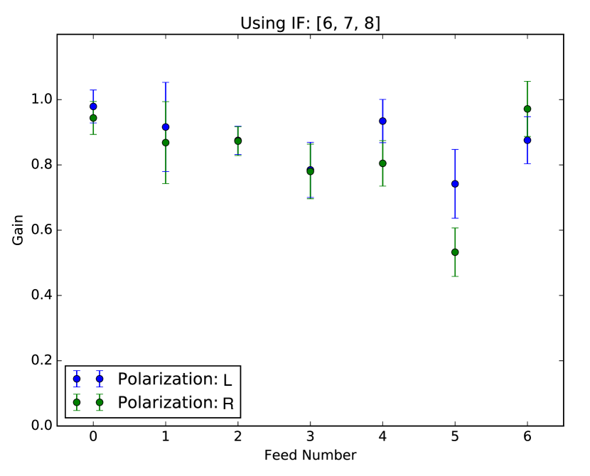
Figure 1: Beam gains for the NH₃ (1,1) spectral windows (IFs 6, 7, and 8) averaged over all Moon observations for each feed and polarization.

The GBT’s VEGAS backend was configured with eight spectral windows, each 23.44 MHz wide. All five NH₃ transitions (1,1) up to (5,5), along with HC₇N $(9-8)$ and CH₃OH ($10_{1}-9_{2}$) $A^{-}$, were observed in seven of the windows across all seven of the KFPA beams. The eighth VEGAS window covered H₂O ($6_{16}-5_{23}$), HC₅N ($8-7$), HC₇N ($19-18$), HNCO ($1_{0,1}-0_{0,0}$), CH₃OH ($12_{2}-11_{1}$) $A^{-}$, and CCS ($2_{0}-1_{0}$) in only the central KFPA beam. The GBT beam has a FWHM of 32$\arcsec$ at the NH₃ (1,1) rest frequency. This VEGAS configuration is the same as that used by the RAMPS survey (Hogge et al., 2018).

In this paper, we present the NH₃ (1,1) and (2,2) emission. Other lines will be presented in future KEYSTONE papers. We also identify H₂O ($6_{16}-5_{23}$) maser emission by eye to include in figures presented in Section 4, but leave the full presentation of those data and a more thorough maser identification technique to White et al. (in prep.). The NH₃ data were reduced using gbtpipe, a Python-packaged version of the standard GBT reduction pipeline. The data were calibrated and output as 3D FITS spectral cubes, with R.A., Dec., and spectral frequency comprising each axis. The on-the-fly observations were mapped to a grid of square pixels with width of 8.8$\arcsec$, which corresponds to $\sim 3.5$ pixels per FWHM beam of the NH₃ (1,1) line. The spectrum corresponding to each spatial pixel was determined using a weighted average of on-the-fly integrations from all seven beams of the K-band Focal Plane array, including those samples with separations less than one FWHM beam size away from a given map pixel. The weighting scheme is a Gaussian-tapered Bessel function, as described in Friesen et al. (2017) following Mangum et al. (2007). This procedure results in data cubes with a resolution of $32^{\prime\prime}$ and the dense sampling from the mapping strategy and multiple receiver feeds produces high-quality maps without discernible scanning patterns in the image or Fourier domain.

The pipeline also subtracts a first-order polynomial fit to the channels on the edges of each scan prior to gridding to remove any shape in the spectral baselines introduced by, e.g., instrumental effects. The pixel size of the final data cubes is 8.8$\arcsec$, with a spectral resolution of 5.7 kHz, or 0.07 km s^-1.

To remove any remaining shape in the spectral baselines, we perform an additional round of per-pixel baseline fitting similar to the method described in Hogge et al. (2018). Namely, a sliding window with a width of 31 channels is used to calculate a “local” standard deviation for every channel in a spectrum. For the 15 channels at each end of the spectrum, the first and last 31 channels are used as the “local” windows, while all other channels are at the center of their “local” window. From the standard deviation distribution of all “local” windows, the central channels belonging to the lowest two quintiles are used for the baseline fit. Thus, channels that belong to an emission line or noise spike are excluded from the baseline fit due to their high “local” standard deviation relative to the non-emission-line channels in the spectrum. Next, polynomials up to a third order are fit to the selected channels. A reduced chi-squared value is then calculated for each of the best-fit polynomials against the full spectrum. Finally, the polynomial with the lowest reduced chi-squared value is subtracted from the original spectrum. This baseline subtraction technique is publicly available, along with the full KEYSTONE data reduction code base. The final baseline-subtracted NH₃ (1,1) and (2,2) data cubes are publicly available.

The system temperatures for the observations were typically $40-50$ K, with a median of $\sim$ 43 K. Figure 2 shows histograms of the RMS noise for the NH₃ (1,1) and (2,2) maps of each cloud. We calculate the RMS using the channels in the best-fit model from our line-fitting procedure (see Section 3.1) with brightness lower than 0.0125 K. While the medians of the RMS distributions range from 0.13 K to 0.2 K, most of the distributions have a peak below 0.15 K. M17 and M16 have slightly higher noise than the other regions since they are the lowest declination sources observed ($\sim-16\degree$ and $-13\degree$, respectively).

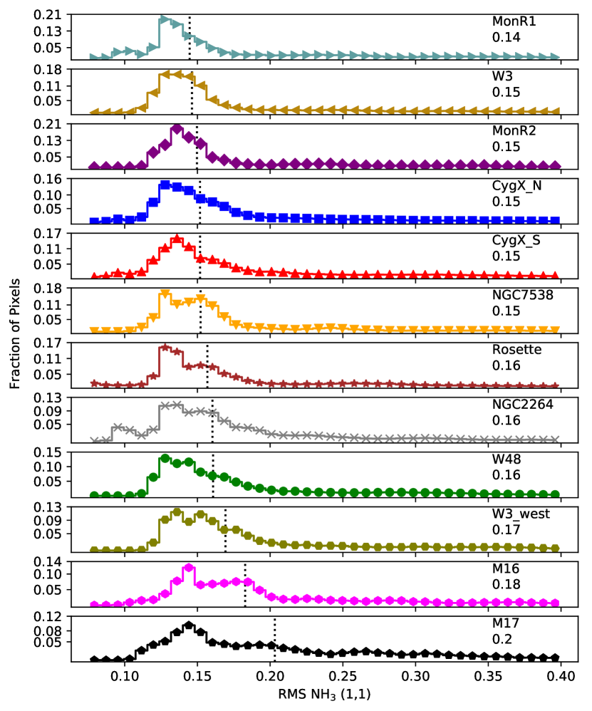
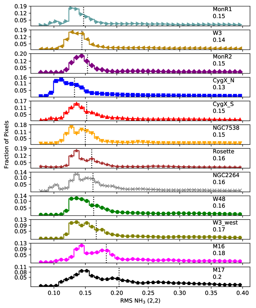
Figure 2: Histograms of the RMS noise for the NH₃ (1,1) (left) and NH₃ (2,2) (right) maps of each cloud. The median of the distribution is displayed as a vertical dotted line, with the corresponding value shown in the upper right corner of each panel. The clouds are ordered from top to bottom by increasing median NH₃ (1,1) RMS noise.

Table 2: KEYSTONE Observed Transitions

Molecule	Transition	Rest Frequency	Number of Beams
		(MHz)
HC5N	($8-7$)	21301.26	1
HC7N	($19-18$)	21431.93	1
CH3OH	($12_{2}-11_{1}$) $A^{-}$	21550.34	1
HNCO	($1_{0,1}-0_{0,0}$)	21981.4706(1)	1
H2O	($6_{16}-5_{23}$)	22235.08	1
CCS	($2_{0}-1_{0}$)	22344.030	1
CH3OH	($10_{1}-9_{2}$) $A^{-}$	23444.78	7
NH3	(1,1)	23694.4955	7
NH3	(2,2)	23722.6336	7
NH3	(3,3)	23870.1296	7
HC5N	($9-8$)	23963.9010	7
NH3	(4,4)	24139.35	7
NH3	(5,5)	24532.92	7

Table 3: Beam Gains

Beam	Polarization L	Polarization R
0	0.979 (0.050)	0.944 (0.051)
1	0.916 (0.137)	0.868 (0.126)
2	0.875 (0.043)	0.873 (0.044)
3	0.785 (0.084)	0.780 (0.084)
4	0.934 (0.066)	0.805 (0.070)
5	0.742 (0.105)	0.533 (0.074)
6	0.876 (0.072)	0.972 (0.085)

Note. — Average beam gains with one-$\sigma$ variations shown in parentheses.

2.3 Herschel Dust Continuum Data

Herschel Space Observatory Level 2.5 data products at 70 $\mu$m, 160 $\mu$m, 250 $\mu$m, 350 $\mu$m, and 500 $\mu$m for each KEYSTONE region were downloaded from the European Space Agency Herschel Science Archive. These maps were originally observed by the Herschel OB Young Stars Survey (Motte et al., 2010) and have spatial resolutions of 8.4$\arcsec$, 13.5$\arcsec$, 18.2$\arcsec$, 24.9$\arcsec$, and 36.3$\arcsec$, respectively. Although the HOBYS team has released dense core and protostar catalogs for MonR2 (Rayner et al., 2017), W3 (Rivera-Ingraham et al., submitted), Cygnus X North (Bontemps et al., in preparation), NGC 6334 (Tigé et al., 2017), and NGC 6537 (Russeil et al. 2019, in press), no catalogs have been yet released for many of the clouds targeted by KEYSTONE. In this paper, we use the Herschel $160-500~{}\mu$m maps to estimate the H₂ column densities and masses of structures identified in the KEYSTONE observations (see Section 3.4). Additionally, we use the 70 $\mu$m maps to identify embedded protostars in each cloud (see Section 3.6).

To estimate H₂ column densities for each region, spectral energy distributions (SEDs) were created by combining the $160-500~{}\mu$m maps for each observed pixel. Full details of the SED-fitting method are described in Singh et al. (2019, in preparation), but are similar to the method applied in all HOBYS papers (see, e.g., Ladjelate et al. in preparation). Here, we provide a brief summary of the process: first, a zero-level offset was added to the 160 $\mu$m map based on Planck observations to account for background continuum emission not included in the Herschel data. The Herschel Level 2.5 products for $250-500~{}\mu$m already have this offset applied, so no additional offsets were added to those maps. Next, all maps were convolved to a resolution of 36.3$\arcsec$ and aligned to the same pixel grid as the 500 $\mu$m map. SEDs were then assembled on a pixel-by-pixel basis and a modified blackbody model of the form $I_{\lambda}=B_{\lambda}(T_{D})\kappa_{\lambda}\Sigma$ was fit to the data, where $I_{\lambda}$ is the surface brightness of the emission, $B_{\lambda}(T_{D})$ is the Planck blackbody function at dust temperature $T_{D}$, and $\kappa_{\lambda}$ is the dust opacity defined as $\kappa_{\lambda}$ = 0.1($\lambda/300\mu$m)^-β cm²/g following Hildebrand (1983) and assuming a gas-to-dust ratio of 100. The dust emissivity, $\beta$, varies between 1.2 and 2.0 for each pixel and is based on Planck-derived dust models (Planck Collaboration et al., 2014) that were resampled to the same pixel grid as the Herschel maps. A stacked histogram showing the $\beta$ distribution across all pixels used for SED fitting in each region is displayed in Figure 3. The $\beta$ distributions vary from cloud to cloud, with the highest values observed in clouds close to the Galactic plane such as W48, M17, and M16. We used Planck-derived values of $\beta$ because the Herschel data include only the portion of the dust SED close to the intensity peak. The position of the intensity peak is a function of both $T_{D}$ and $\beta$ (e.g., $\lambda_{peak}=1.493/T_{D}(3+\beta)$ for a modified blackbody, Elia & Pezzuto, 2016) and it is not possible to remove the degeneracy between these two parameters unless data at longer wavelengths, where $I_{\nu}\propto\lambda^{-\beta}$, are used. Since the Planck data include observations down to 850 $\mu$m, they are more capable of constraining $\beta$ than the Herschel data.

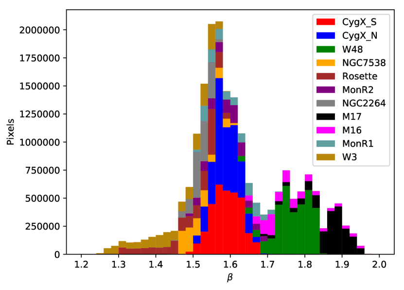
Figure 3: Stacked histogram of the dust emissivity, $\beta$, used for SED fitting of each pixel in the Herschel dust continuum maps for all clouds observed by KEYSTONE. The $\beta$ values are from Planck-derived dust models (Planck Collaboration et al., 2014) that have been resampled to the same pixel grid as the Herschel data.

The gas surface mass density, $\Sigma$, and dust temperature were left as free parameters during the fitting procedure. The resulting best-fit model’s $\Sigma$ was converted to H₂ column density, $N(H_{2})$, using $\Sigma=\mu_{H}m_{H}N(H_{2})$, where $\mu_{H}$=2.8 is the mean molecular weight per hydrogen molecule, which assumes the relative mass ratios of hydrogen, helium, and metals are 0.71, 0.27, and 0.02, respectively (see, e.g., Appendix A in Kauffmann et al., 2008), and $m_{H}$ is the mass of a hydrogen atom. The SED fitting procedure failed to converge for a small fraction of pixels where the dust continuum emission was saturated. The percentage of affected pixels for the KEYSTONE clouds affected are: M17 ($0.09\%$), W48 ($0.008\%$ of pixels), Cygnus X North ($0.006\%$ of pixels), NGC7538 ($0.01\%$ of pixels), W3 ($0.01\%$ of pixels), and MonR2 ($0.001\%$ of pixels). For the affected pixels, we replace their values with the median column density of the ten closest pixels with reliable SED fits. As such, this is likely a lower limit to the true column density for those pixels. Any dendrogram-identified leaf (see Section 3.3) that overlaps with one of these affected pixels is also flagged in all catalogs and analyses. The number of leaves in each cloud that include affected pixels are: M17 (1 of 38 leaves), W48 (1 of 100 leaves), Cygnus X North (2 of 200 leaves), NGC7538 (1 of 73 leaves), and W3 (2 of 84 leaves).

The main difference between the column densities derived in this paper and those of the HOBYS collaboration (Ladjelate et al. in preparation) involve the assumptions on $\beta$. Specifically, the HOBYS column density maps assume $\beta=2$ for all pixels while we use $1.2\leq\beta\leq 2.0$ based on Planck dust models that constrain $\beta$ on large spatial scales (Planck Collaboration et al., 2014). Our lower values of $\beta$ result in comparatively lower column densities in our maps. For instance, the HOBYS team has released the H₂ column density maps and core/protostar catalog for MonR2 (Rayner et al., 2017). We find that the Rayner et al. (2017) column densities are on average a factor of $\sim 2.5$ higher than those derived in this paper. Although the higher column densities in the HOBYS maps would lead to larger structure masses in our analysis, we discuss in Section 3.4 that the method used to convert the column densities into structure masses is likely a larger source of uncertainty than the $\beta$ assumption. Moreover, we also recovered 22 of the 28 ($\sim 79\%$) protostars identified by Rayner et al. (2017), with the six discrepant sources located in the central MonR2 hub that is bright at 70 $\mu$m. This suggests that our protostar extraction is likely confusion limited in bright hubs, but can efficiently recover sources that are more isolated.

2.4 JCMT C¹⁸O Data

C¹⁸O $(3-2)$ data cubes observed by the HARP-ACSIS spectrometer on the James Clerk Maxwell Telescope (JCMT) were obtained from the JCMT Science Archive, which is hosted by the Canadian Astronomy Data Centre. Of the eleven clouds observed by KEYSTONE, six were found to have publicly available C¹⁸O $(3-2)$ data cubes in the JCMT Science Archive: Cygnus X North, Cygnus X South, M16, M17, NGC7538, and W3. The native spectral resolution of the C¹⁸O $(3-2)$ cubes is $\sim$ 0.056 km s^-1 and the spatial resolution is 15.3$\arcsec$. To match better the spatial and spectral resolution of our NH₃ observations and improve sensitivity, we smoothed the C¹⁸O $(3-2)$ maps to a spatial resolution of 32$\arcsec$ and spectral resolution of 0.11 km s^-1. In Section 4.3, we describe how Gaussian line fitting of these data cubes is used to estimate the external, turbulent pressure on the ammonia structures observed by KEYSTONE.

3 Analysis and Results

3.1 NH₃ Line Fitting

The NH₃ (1,1) and (2,2) lines were used to estimate the excitation temperature ($T_{ex}$), kinetic gas temperature ($T_{K}$), centroid velocity ($V_{LSR}$), velocity dispersion ($\sigma$), and para-NH₃ column density ($N_{para-NH_{3}}$) for each pixel. We adopted the line fitting method of the Green Bank Ammonia Survey (GAS) described in Friesen et al. (2017), which uses the coldammonia model in the pyspeckit Python package (Ginsburg & Mirocha, 2011) to generate model ammonia spectra under the assumptions of LTE and a single velocity component along the line of sight. While most of the KEYSTONE spectra are well characterized by a single velocity component, we do see signs of multiple velocity components that are closely separated along the spectral axis in regions of W48 and M17. For those spectra, our single velocity component fitting will produce a best-fit model that has a broadened line width to account for the larger width of the emission line features in the spectrum. In a future KEYSTONE paper, we plan to implement a multiple velocity component fitting method that will robustly identify spectra with more than one velocity component and estimate better the line widths for those spectra (Keown et al., in preparation).

The GAS line-fitting pipeline was applied to all pixels with NH₃ (1,1) signal-to-noise ratio (SNR) $>$ 3, where SNR is measured from the ratio of peak emission-line intensity to the rms of the off-line channels in the spectrum. In addition to the minimum SNR threshold, pixels were excluded from our final parameter maps if they did not meet the following constraints on the best-fit model parameters and uncertainties:

1. 5 K $<T_{K}<$ 40 K (outside this range, the NH₃ (1,1) and (2,2) lines cannot constrain $T_{K}$);

2. 0.05 km s^-1 $<\sigma<$ 2.0 km s^-1 (below 0.05 km s^-1 is unrealistic since our channel width is only $\sim$ 0.07 km s^-1; above 2.0 km s^-1 is uncharacteristic of NH₃ (1,1) emission in the observed star-forming environments (e.g., Pillai et al., 2011; Olmi et al., 2010) and likely indicates the presence of strong outflows or multiple velocity components along the line of sight);

3. $N_{para-NH_{3}}<10^{16}$ cm^-2 (above $10^{16}$ cm^-2 is uncharacteristic of NH₃ emission in the observed star-forming environments (e.g., Olmi et al., 2010));

4. $T_{K,err}<$ 5 K;

5. $\sigma_{err}<$ 2.0 km s^-1;

6. $V_{LSR,err}<$ 1 km s^-1;

7. $(\log{N_{para-NH_{3}}})_{err}<2$ ;

where $4-7$ are included to cull fits that were unable to converge.

The final parameter maps for each region are shown in Figures 4-15. To compare each region’s ammonia emission to its dust continuum emission, we also plot Herschel H₂ column density contours overtop the ammonia parameter maps presented in Figures 4-15. The ammonia emission tends to occur where total extinction in the V band ($A_{V}$) is larger than $\sim 6-8$ mag.

A comparison of the $T_{K}$ and $\sigma$ histograms for each region is presented in Figure 16. Although the $T_{K}$ distributions are consistent for most of the regions, there are significant temperature differences between the regions with the lowest temperatures (MonR1 and W3-west) compared to the highest temperature regions (M17 and MonR2). Similarly, the $\sigma$ distributions are fairly consistent across regions, with peak values of $0.3-0.7$ km s^-1. There are several regions (NGC7538, W48, M17), however, that have a tail of pixels with large line widths $>$ 1 km s^-1. These large line width tails are likely due to a higher fraction of pixels with strong outflows or multiple velocity components along the line of sight.

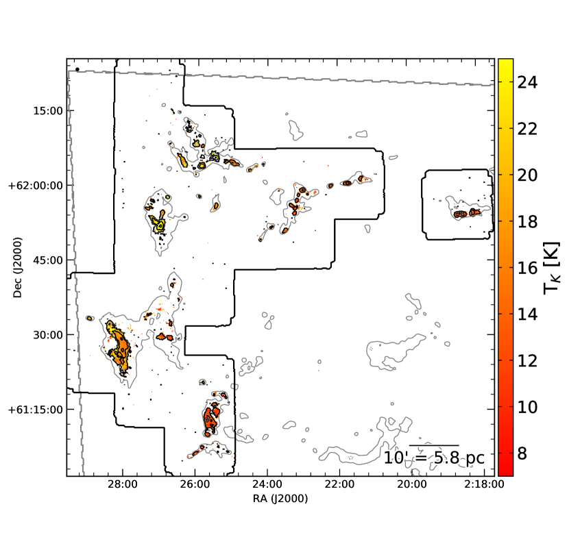
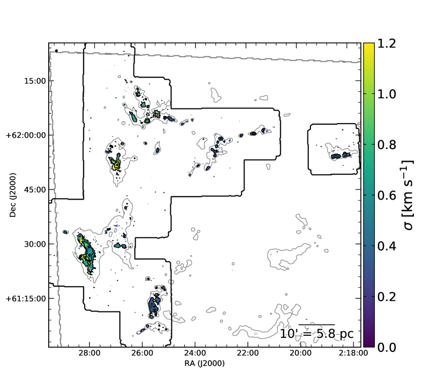
Figure 4: Kinetic temperature (top) and NH₃ (1,1) velocity dispersion (bottom) derived from NH₃ (1,1) and (2,2) line fitting of the W3 observations. The black contours show the NH₃ (1,1) integrated intensity at 1.0, 3.5, and 10 K km s^-1. The solid and dotted grey contours outline H₂ column densities of $2.8\times 10^{21}$ cm^-2 and $9.4\times 10^{21}$ cm^-2, respectively, which are equivalent to a total extinction in the V band of A${}_{V}=3$ mag and 10 mag. The 32$\arcsec$ beam size is shown as a black dot in the upper left corner of each plot. The thick black and gray lines outline the KEYSTONE and Herschel mapping boundaries, respectively.

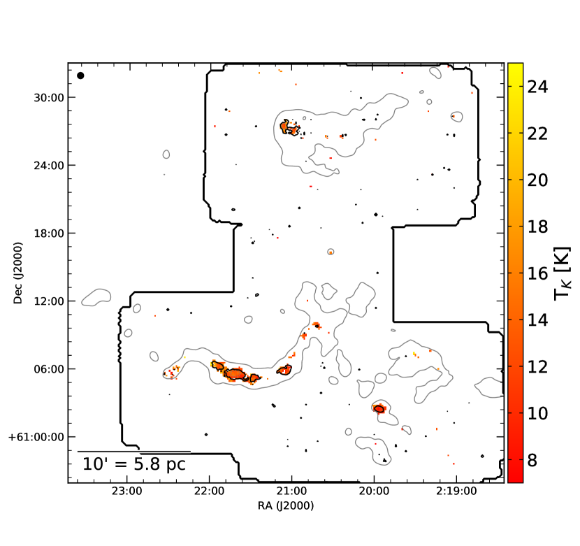
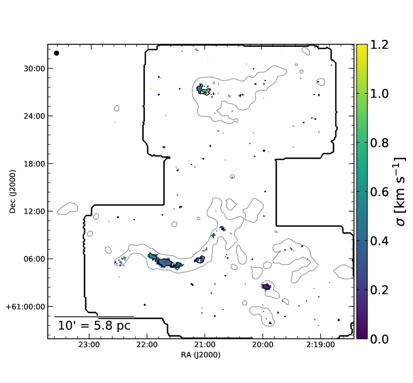
Figure 5: Same as Figure 4 for W3-west.

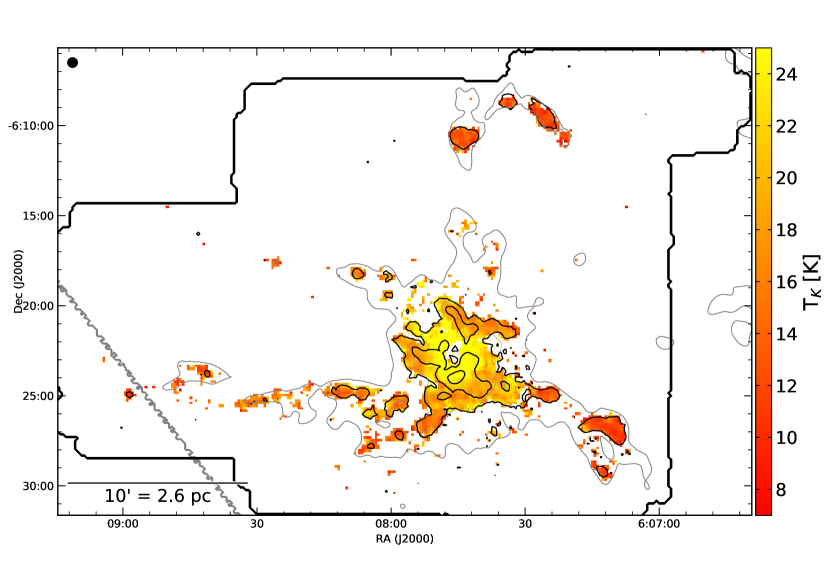
Figure 6: Same as Figure 4 for MonR2.

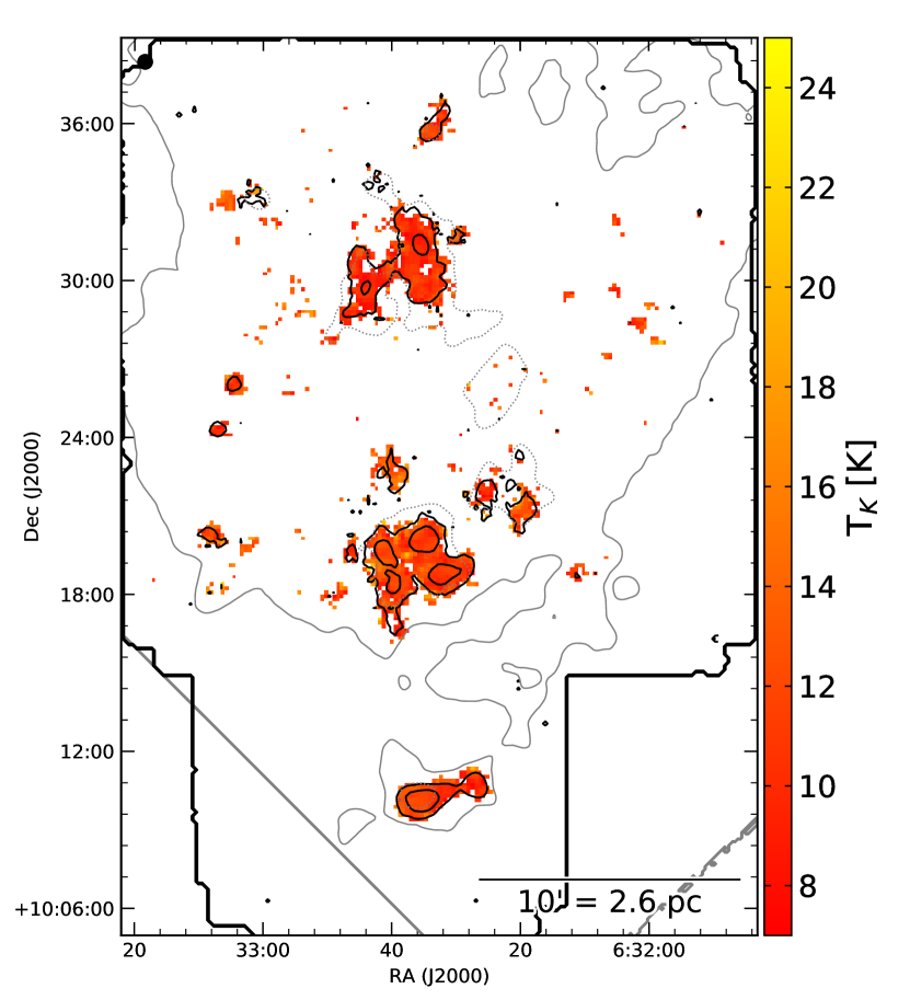
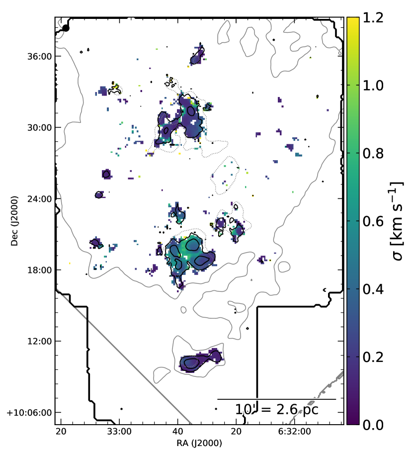
Figure 7: Same as Figure 4 for MonR1.

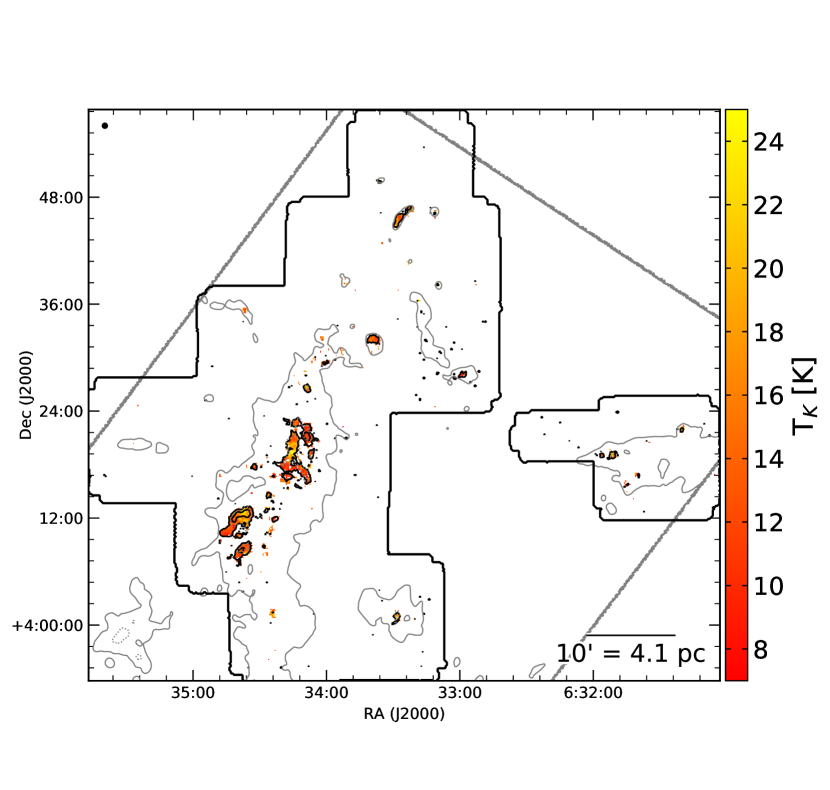
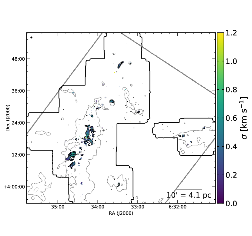
Figure 8: Same as Figure 4 for Rosette.

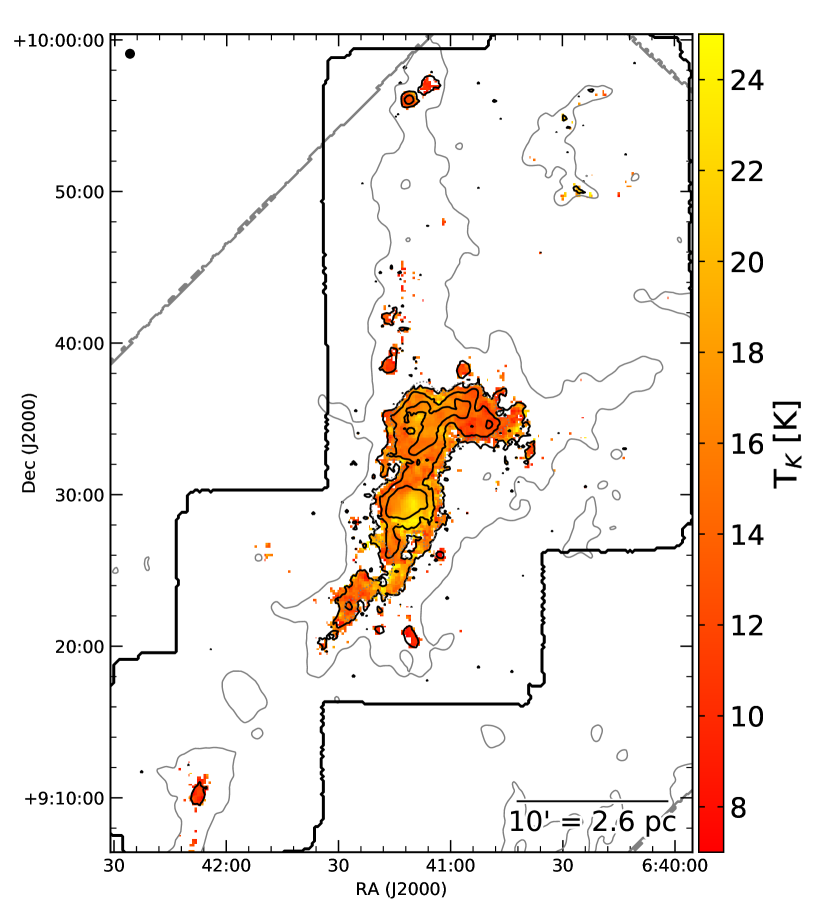
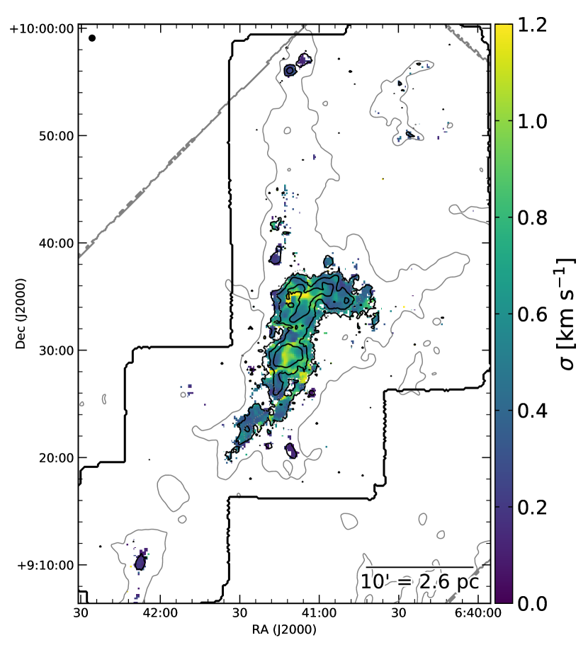
Figure 9: Same as Figure 4 for NGC2264.

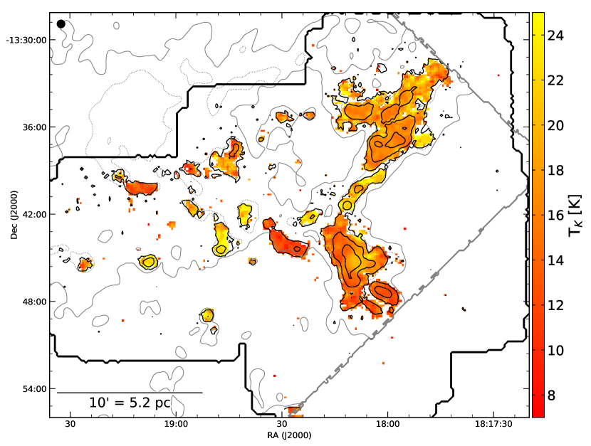
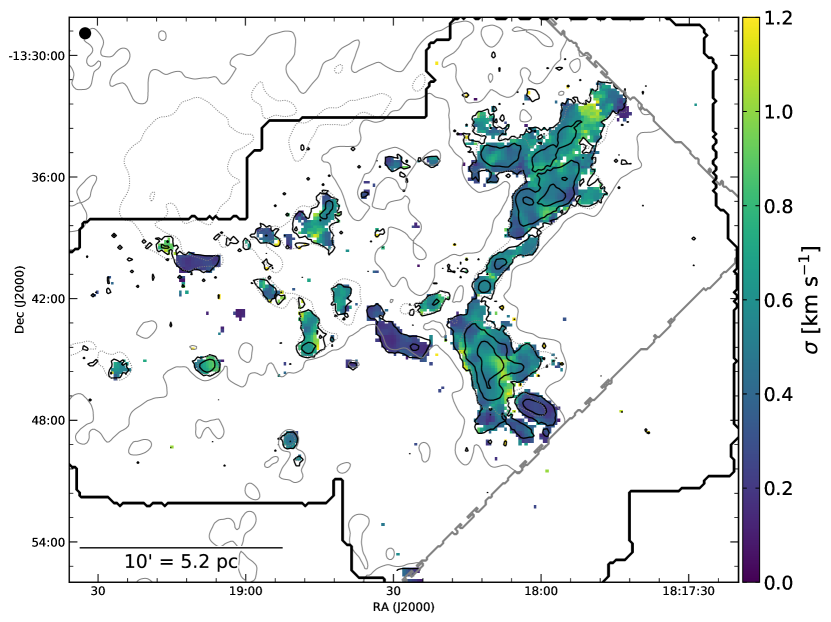
Figure 10: Same as Figure 4 for M16. The solid and dotted grey contours outline H₂ column densities of $5.6\times 10^{21}$ cm^-2 and $9.4\times 10^{21}$ cm^-2, respectively, which are equivalent to a total extinction in the V band of A${}_{V}=6$ mag and 10 mag.

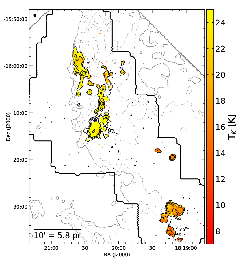
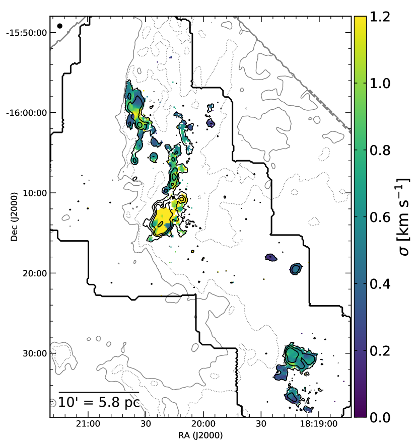
Figure 11: Same as Figure 4 for M17. The solid and dotted grey contours outline H₂ column densities of $7.5\times 10^{21}$ cm^-2 and $9.4\times 10^{21}$ cm^-2, respectively, which are equivalent to a total extinction in the V band of A${}_{V}=8$ mag and 10 mag.

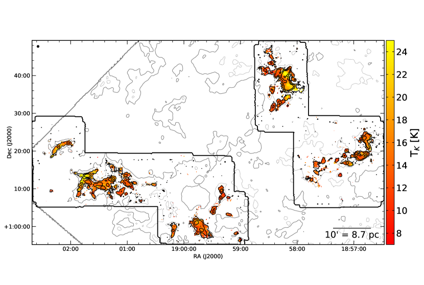
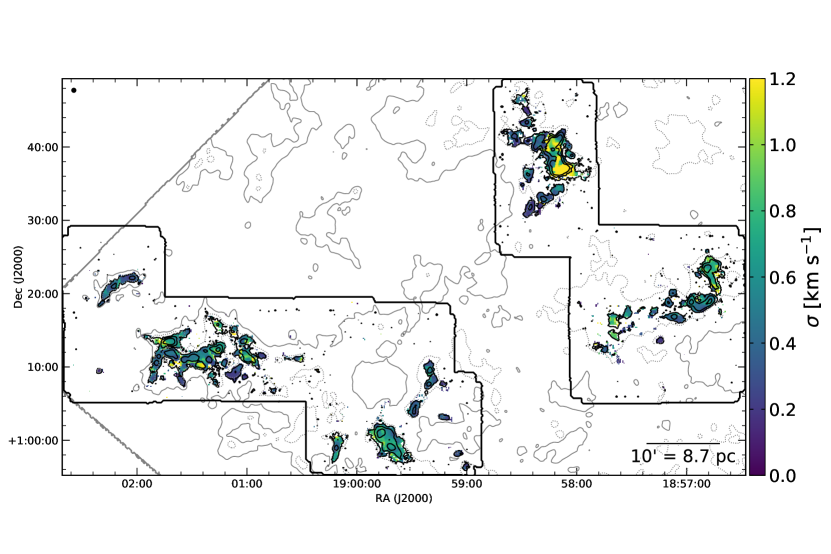
Figure 12: Same as Figure 10 for W48.

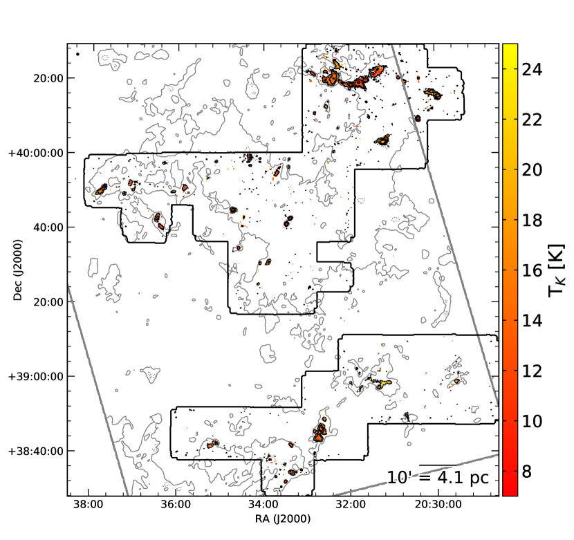
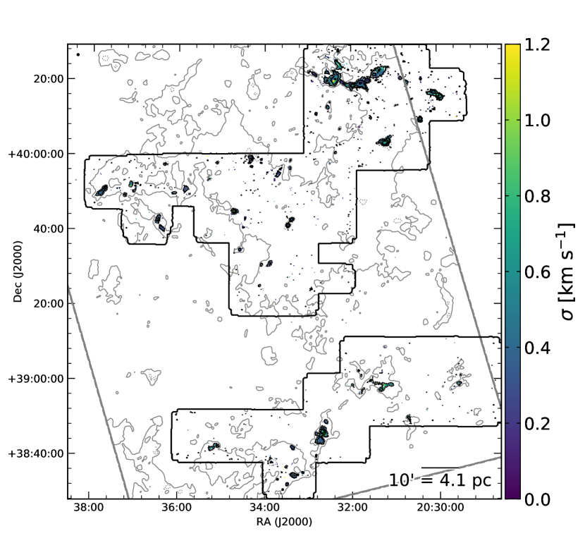
Figure 13: Same as Figure 4 for Cygnus X South. The solid and dotted grey contours outline H₂ column densities of $4.7\times 10^{21}$ cm^-2 and $9.4\times 10^{21}$ cm^-2, respectively, which are equivalent to a total extinction in the V band of A${}_{V}=5$ mag and 10 mag.

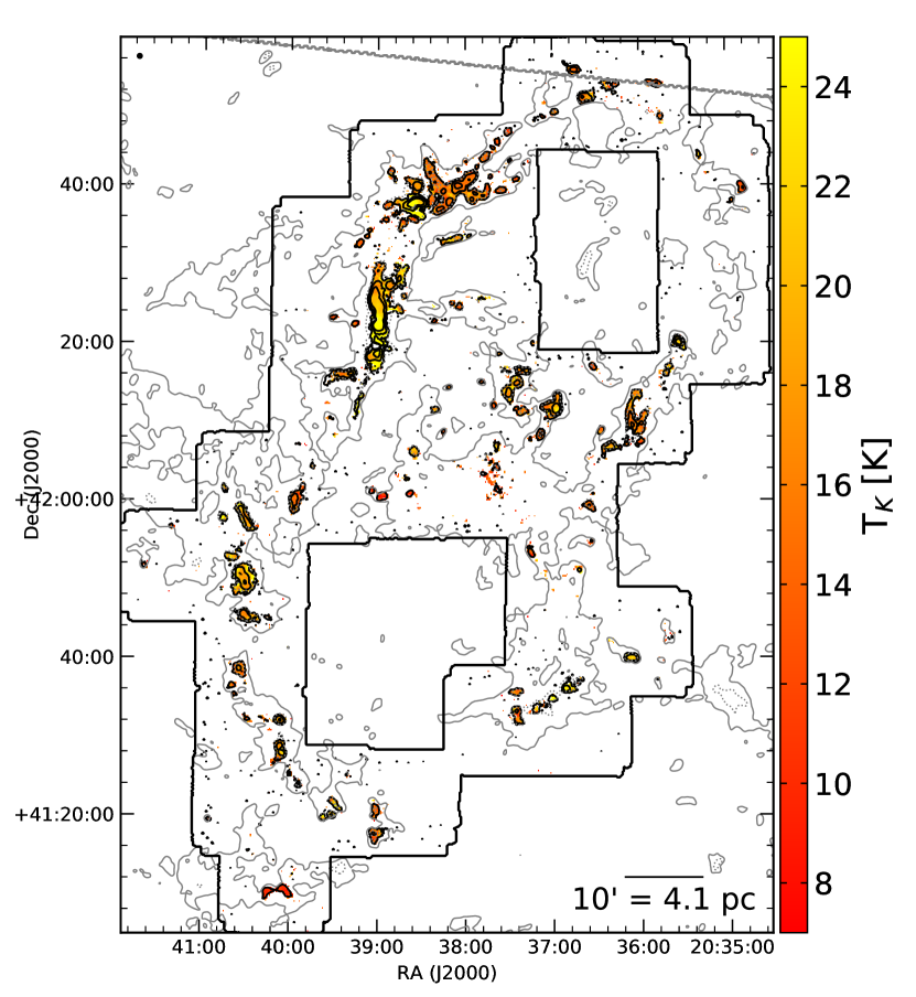
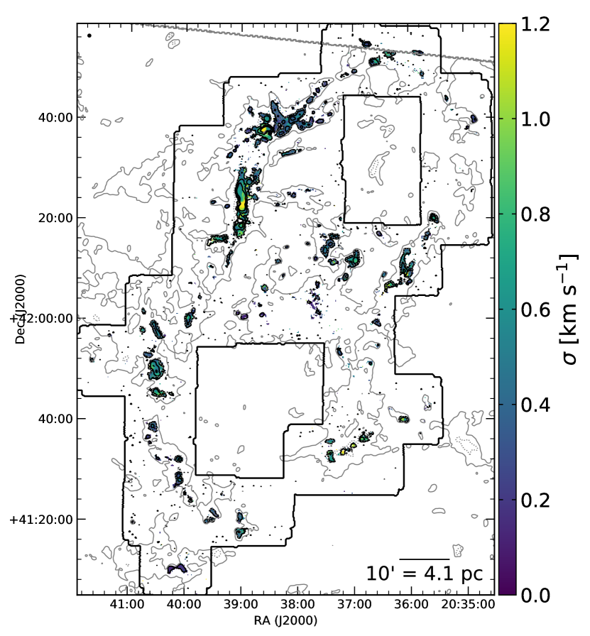
Figure 14: Same as Figure 13 for Cygnus X North.

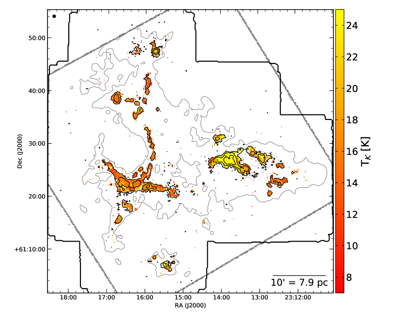
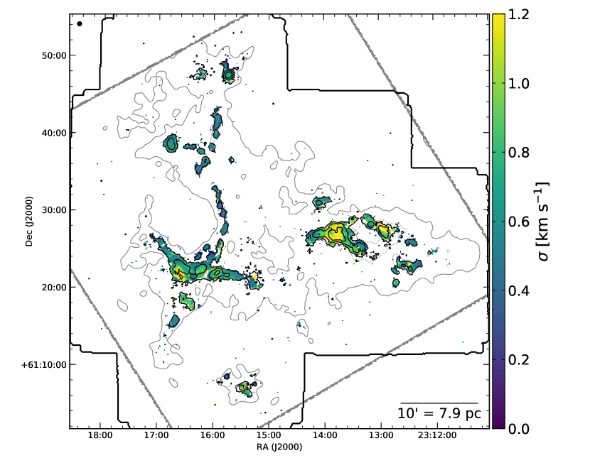
Figure 15: Same as Figure 4 for NGC7538.

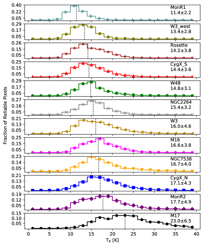
Figure 16: Histograms of kinetic temperature (left) and NH₃ (1,1) velocity dispersion (right) for the reliably fit pixels in each region. The median and median absolute deviation of each distribution is printed in the top right corner of each panel. The clouds are ordered from top to bottom by increasing median kinetic temperature.

3.2 NH₃ (1,1) Integrated Intensity Maps

The best-fit models from the NH₃ (1,1) line fitting described in Section 3.1 were used to identify the channels to integrate for producing NH₃ (1,1) integrated intensity maps. Namely, the spectral channels in the best-fit models that were brighter than 0.0125 K were included in the integration. This threshold was selected to include only the channels that are part of an emission line in the best-fit models. Since the off-line channels in a pyspeckit model are slightly above zero due to machine precision, the threshold of 0.0125 K provides a conservative distinction between emission-line and off-line channels in the models. For pixels that did not have any channels above that brightness criterion, we use the set of spectral channels centered on the mean cloud centroid velocity with a range defined by the mean cloud line width. In addition, we blank all pixels within three pixels from the map edges since they have lower coverage by the KFPA and typically have higher noise. Figures 17-28 show the final NH₃ (1,1) integrated intensity maps for each region.

3.3 Identifying NH₃ Structures with Dendrograms

The hierarchical nature of molecular clouds (e.g., Falgarone & Puget, 1986; Lada, 1992; Bonnell et al., 2003) warrants a structure-identification method that handles features with different sizes, shapes, and spatial scales. Dendrograms are a proven identification method that excel at identifying such hierarchical features in both continuum (e.g., Kirk et al., 2013b; Könyves et al., 2015) and molecular line emission observations (e.g., Rosolowsky et al., 2008; Goodman et al., 2009; Lee et al., 2014; Seo et al., 2015; Friesen et al., 2017; Keown et al., 2017) and simulations (Boyden et al., 2016; Koch et al., 2017; Boyden et al., 2018). This ability arises from the tree-diagram architecture of dendrogram algorithms, which first identifies the pixels in a map that represent local maxima. Next, structures are assembled around the local maxima by joining nearby fainter pixels. These top-level leaves are grown until they either merge with another nearby leaf, at which point they are connected by a branch, or reach a pre-defined noise threshold below which no more pixels are added to the structure. The lowest-level structures above this noise threshold that are connected to branches are known as trunks.

Due to the hyperfine structure of NH₃ (1,1) emission, each hyperfine group would be detected as a distinct structure in a 3D dendrogram extraction of the KEYSTONE spectral cubes. To “remove” the hyperfine structures of NH₃ (1,1), some authors have created a single-Gaussian cube from the line width, peak brightness temperature, and centroid velocity measured from the NH₃ (1,1) emission (e.g., Friesen et al., 2017; Keown et al., 2017). Such a single-Gaussian cube attempts to represent how the ammonia emission would appear without hyperfine splitting. Unless the ammonia emission is fit using a model with multiple velocity components along the line of sight, however, the output single-Gaussian cube does not account for emission with multiple velocity components. Instead, a robust multiple velocity component line-fitting method would first need to be applied to the data to take full advantage of a 3D dendrogram extraction of NH₃ (1,1) cubes. The multiple velocity component models would then allow for the creation of a “multi-Gaussian” cube that removes the hyperfine structures of NH₃ (1,1) while preserving the presence of multiple velocity components along the line of sight. Although a multiple velocity component NH₃ (1,1) line-fitting method has been developed in another KEYSTONE paper (Keown et al. 2019, submitted), the analysis presented here neglects multiple velocity components along the line of sight.

Here, we instead perform a dendrogram analysis of the NH₃ (1,1) integrated intensity maps described in Section 3.2. When the observed emission has only a single velocity component along the line of sight, a 2D dendrogram extraction of the integrated intensity maps will produce similar results as a 3D extraction of the full emission cube. Since the majority of the KEYSTONE observations appear to lack multiple velocity components, a 2D analysis is warranted. We defer a 3D dendrogram analysis of the ammonia data to a future KEYSTONE paper.

The astrodendro Python package was applied to the integrated intensity map for each region. For consistency with the ammonia dendrogram analyses by Friesen et al. (2016) and Keown et al. (2017), we chose the following values for the dendrogram algorithm input parameters:

• min_value = 5 $\times$ RMS, where RMS is the rms noise measured in a region of the integrated intensity map where no emission was detected. For clouds with highly variable noise in the integrated intensity map, the RMS was calculated using an emission-free region representative of the highest noise portion of the map. While this conservative approach may leave some low brightness sources undetected, it reduces the amount of spurious noise sources detected by the dendrogram. min_value is the lowest intensity a pixel can have to be joined to a neighboring structure.

• min_delta = 2 $\times$ RMS, where RMS is the same as described for min_value. min_delta is the minimum difference in brightness between two structures before they are merged into a single structure.

• min_npix = 10 pixels. min_npix is the minimum number of pixels a structure must contain to remain independent. This parameter prevents noise spikes from being identified as sources.

After running the dendrogram algorithm on the maps, we cull leaf sources from our final catalog that do not meet the following criteria:

• The total area of the leaf, in terms of all the pixels associated with it, must be larger than the total area of the GBT beam. This criterion ensures further that small noise spikes are excluded from our final catalog and analyses.

• The leaf contains at least one pixel that was reliably fit by the NH₃ line fitting method described in Section 3.1. Here, a reliably fit pixel is one that passes the seven constraints listed in Section 3.1.

Figure 29 shows an example tree diagram for the dendrogram extraction of the MonR2 region. Leaves that do not pass our selection criteria are shown as black vertical lines, while robust leaves are shown in blue and parent structures are shown in red. The tree diagram shows that our selection criteria preferentially cull isolated leaves that are not associated with larger-scale parent structures and are likely noise spikes in the map. Table 4 provides a sample catalog of the leaves that pass our selection criteria in W3-west. Similar catalogs for all eleven KEYSTONE regions are available online. Of the 970 total leaves identified by the dendrograms in each region, the final catalog includes a total of 856 leaves ($\sim 88\%$) that passed all of the culling criteria. Figures 17-28 show the final catalog leaf masks overlaid atop the NH₃ (1,1) integrated intensity map for each region. These masks show the full extent of all pixels associated with each leaf. For the remainder of the paper, we refer to leaves and clumps synonymously since the ammonia-identified leaves represent the dense gas structures from which new stars may form.

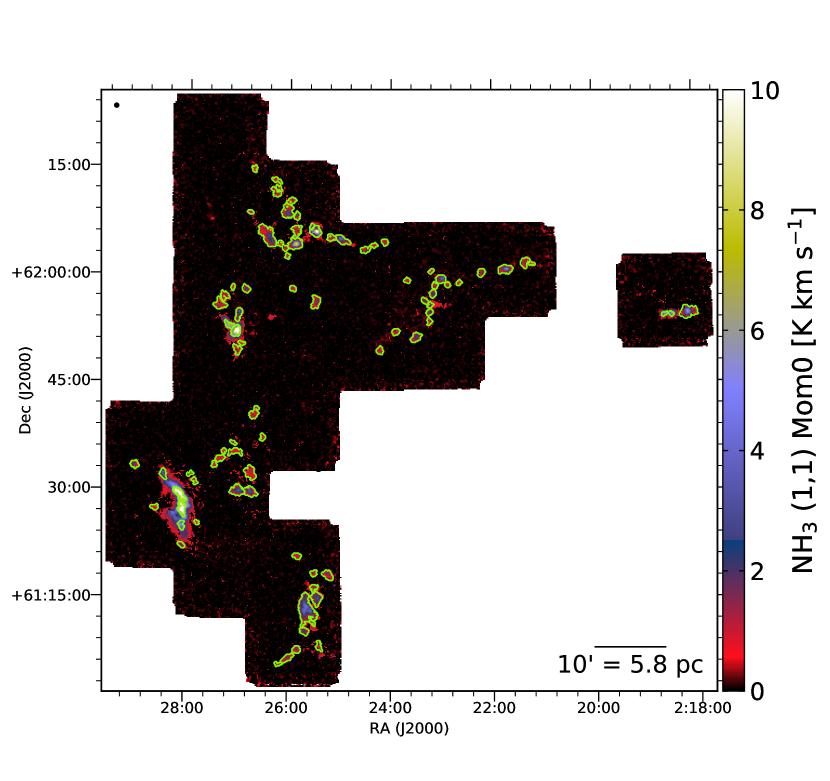
Figure 17: NH₃ (1,1) integrated intensity map for W3. Green contours outline leaves identified by a dendrogram analysis of the map that passed the culling criteria listed in Section 3.3.

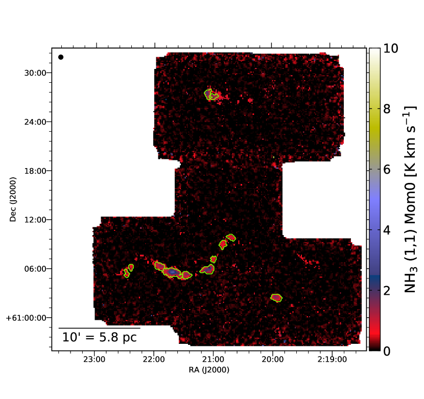
Figure 18: Same as Figure 17 for W3-west.

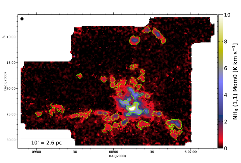
Figure 19: Same as Figure 17 for MonR2.

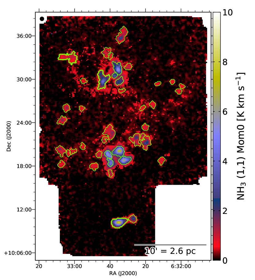
Figure 20: Same as Figure 17 for MonR1.

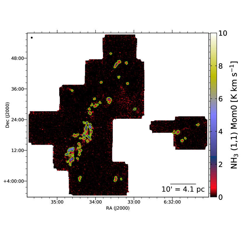
Figure 21: Same as Figure 17 for Rosette.

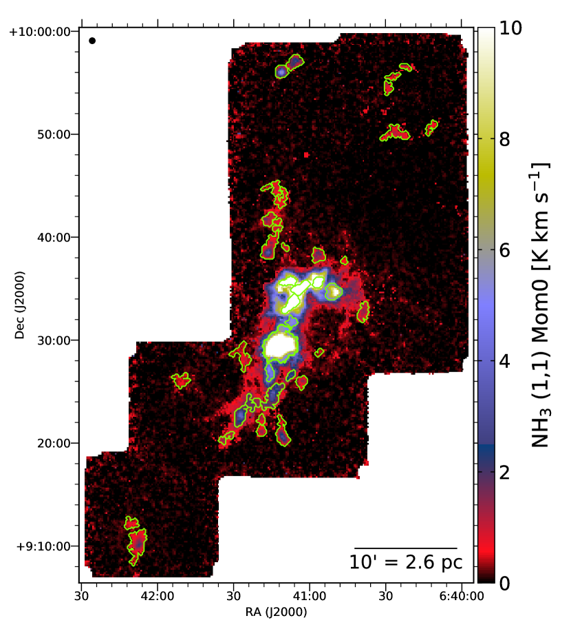
Figure 22: Same as Figure 17 for NGC2264.

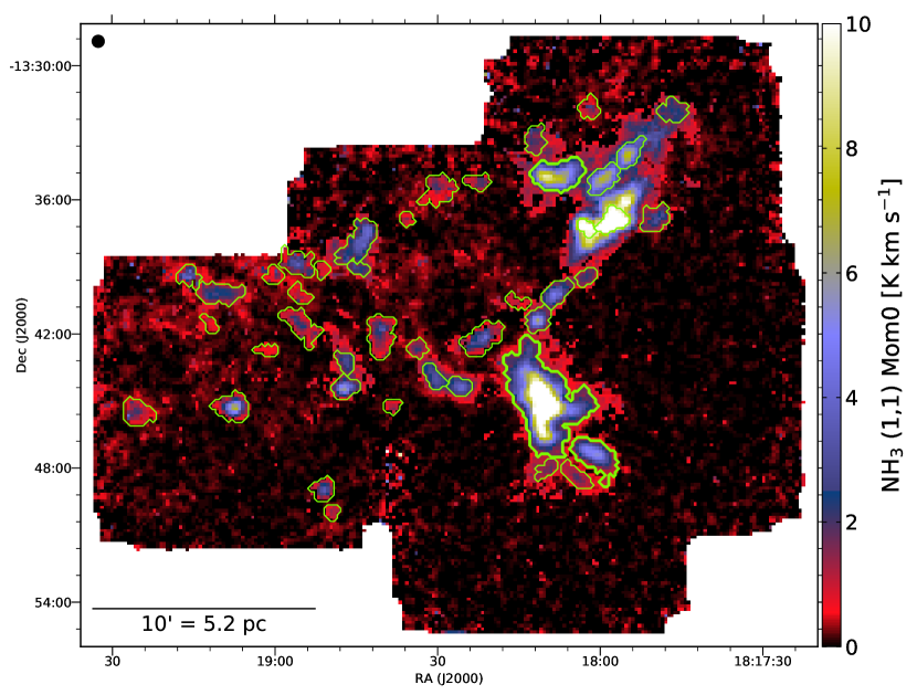
Figure 23: Same as Figure 17 for M16.

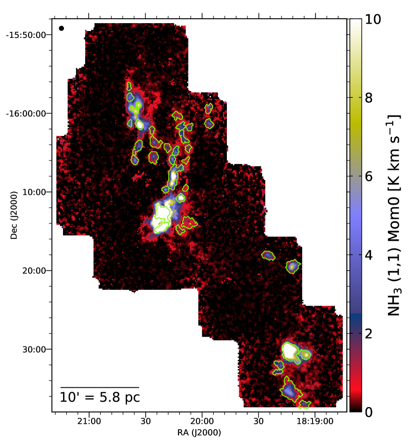
Figure 24: Same as Figure 17 for M17.

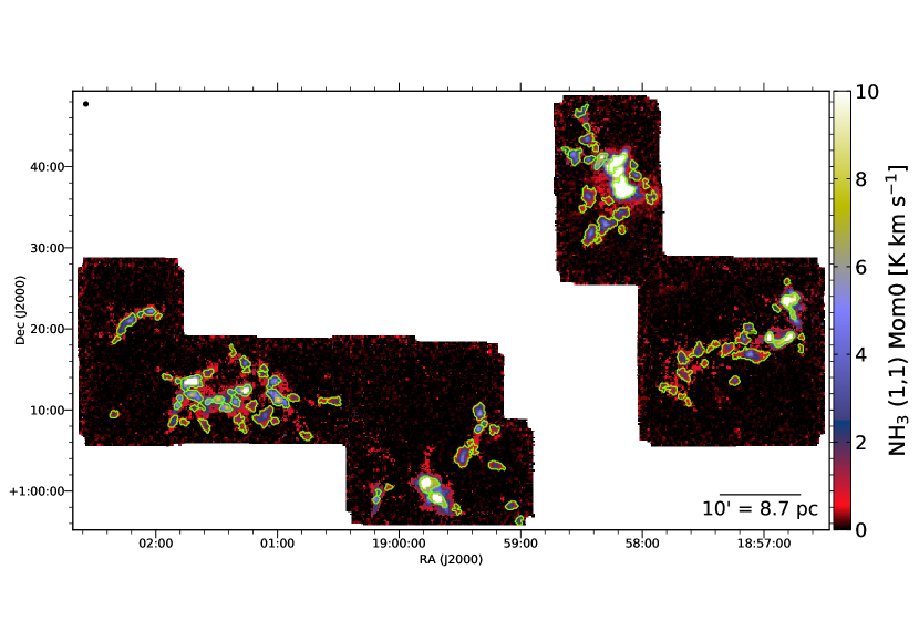
Figure 25: Same as Figure 17 for W48.

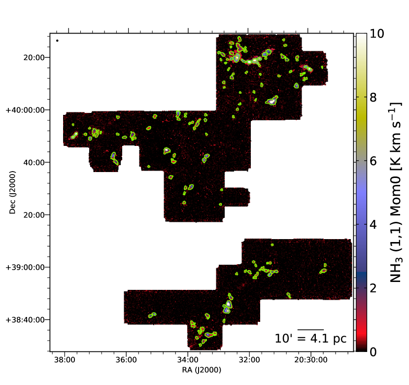
Figure 26: Same as Figure 17 for Cygnus X South.

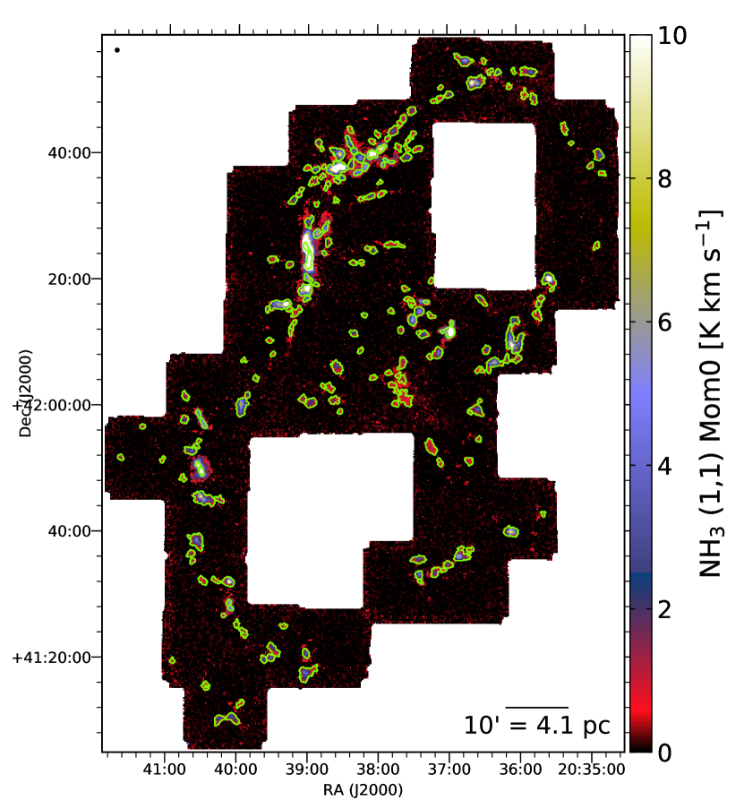
Figure 27: Same as Figure 17 for Cygnus X North.

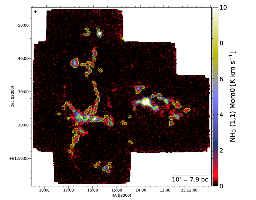
Figure 28: Same as Figure 17 for NGC7538.

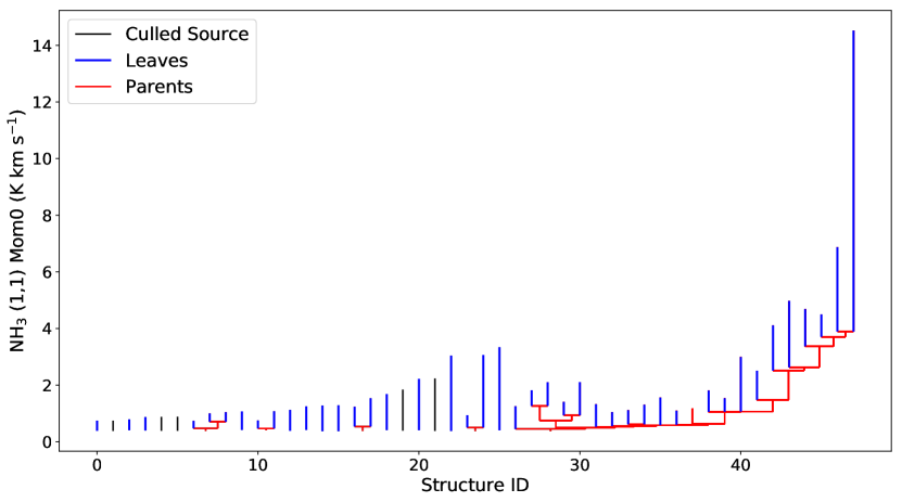
Figure 29: Dendrogram tree diagram for MonR2 showing the peak intensity for each structure identified. Leaves are shown in blue and branches are shown in red. Leaves that were culled based on the selection criteria described in Section 3.3 are shown in black. Leaves that are red denote culled leaves that are part of a branch with an accepted leaf.

3.4 Determining Leaf Radii and Masses

The effective radii of the ammonia-identified leaves were estimated using the area of the leaf masks identified by the dendrogram analysis. Following Kauffmann et al. (2013), we adopt $R_{eff}=(A/\pi)^{1/2}$ as the effective radius, where $A$ is the area of all pixels in the leaf’s mask on the position-position plane. Rosolowsky & Leroy (2006) showed that this area-based radius formulation becomes inaccurate for structures with low SNR and sizes much larger or smaller than the beam size. Although we do enforce that leaves are comprised of pixels with at least 5$\sigma$ detections (see Section 3.3) and limit structures to being larger than the beam size, $R_{eff}$ may still be susceptible to such biases. To estimate the uncertainties on our measured radii, we use the method described by Chen et al. (2019a), which uses the radii of the largest circle that fits inside the leaf boundary as the leaf’s radii lower limit and the radii of the smallest circle that encompasses the leaf as its radii upper limit. The corresponding uncertainties on $R_{eff}$ based on these upper and lower limits are listed in Table 4. The uncertainties range from $0.1\%$ to $153\%$ of $R_{eff}$, with a median of $35\%$.

Masses for the ammonia-identified leaves were estimated by summing all the H₂ column density for the pixels inside each leaf’s mask. The integrated column densities are then converted to mass assuming the distances to each region listed in Table 1 and a mean molecular weight per hydrogen molecule $\mu_{H}$ = 2.8. In Cygnus X and MonR2, a small number of leaves (six in Cygnus X North, 14 in Cygnus X South, and one in MonR2) fall outside the boundaries of our H₂ column density maps. Those sources are, therefore, excluded from our analyses that require a mass determination.

Summing all the column density within the leaf boundaries is likely an upper limit on the mass of the structure. Conversely, a lower limit on the structure’s mass can be obtained by using the “clipping” technique described in Rosolowsky et al. (2008) and Chen et al. (2019a). Namely, before summing the column density pixels within the leaf boundary, the lowest column density pixel’s value is subtracted from all other pixels. This method aims to remove contributions to the structure’s observed column density from background sources, but is likely over-estimating the true background contribution in most cases. As such, we adopt the regular integrated column density masses throughout this paper, but show the range the mass could be assuming the “clipped” mass is a lower limit. The clipped masses are also displayed in Table 4 alongside the integrated column density masses. The clipped masses are typically a factor of $\sim 5$ (median) lower than the integrated column density masses.

The left panel of Figure 30 shows the effective radii versus mass for all leaves in our final catalog. A power-law fit to the radius versus mass distribution reveals a best-fit slope of 2.43 $\pm$ 0.45, which is consistent with the value of 2 expected for clumps of constant surface density and the value of 3 expected for clumps of constant volume density. The data were fit using a Markov Chain Monte Carlo (MCMC) sampler. The MCMC sampling used an orthogonal least-squares likelihood function and uniform priors on the power-law slope and intercept. The best-fit model parameters were taken to be the medians of the accepted parameters in the MCMC chain, while the uncertainty on the best-fit parameters was taken to be the standard deviations of the accepted parameter distributions.

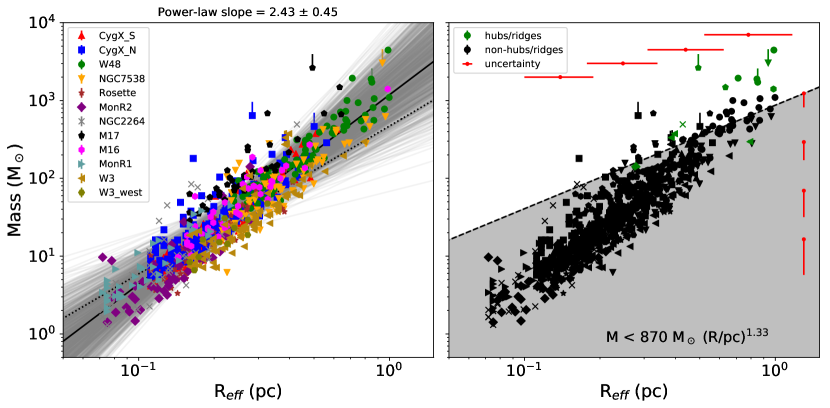
Figure 30: Left: effective radius versus mass for the leaves identified in each region. The solid black line shows the best power-law fit to the data using an MCMC sampler. The grey lines show 1000 random selections from the full MCMC chain. The dotted line shows a power-law slope of 1.9 (Larson, 1981) for comparison. Right: effective radius versus mass for hubs (green) and non-hubs (black) identified in each region (see Section 4.1 for discussion of hubs). The dashed black line denotes the empirically-derived threshold for massive star formation determined by Kauffmann & Pillai (2010). The red dots with errorbars show the median mass and radius uncertainties in different bins along each axis. All other errorbars show leaves that have mass lower limits due to saturated pixels in the H₂ column density map (see Section 2.3).

3.5 Virial Analysis

To estimate the virial stability of the ammonia-identified leaves, we adopt the virial analysis method described in Keown et al. (2017), which uses the ammonia-derived line widths to derive a virial mass ($M_{vir}$) for each structure given by:

$$M_{vir}=\frac{5\sigma^{2}R}{aG}$$ (1)

where $\sigma$ is the velocity dispersion of the core (including both the thermal and nonthermal components), R is the core radius, G is the gravitational constant, and

$$a=\frac{1-k/3}{1-2k/5}$$ (2)

is a term which accounts for the radial power-law density profile of a core, where $\rho(r)\propto r^{-k}$ (Bertoldi & McKee, 1992). $M_{vir}$ represents the mass that a structure with a given radius and internal kinetic energy would have if it were in virial equilibrium when considering only its gravitational potential and kinetic energies. We also assume that the structure is in a steady state, spherical, isothermal, and has a radial power-law density profile of the form: $\rho(r)\propto r^{-1.5}$. Our density profile assumption is motivated by recent observations that found $\rho(r)\propto r^{-1.5\pm 0.3}$ for the inner regions of dense cores (e.g., Kurono et al., 2013; Pirogov, 2009) and is likely a more accurate choice than the Gaussian density profile chosen in previous virial analyses (e.g., Pattle et al., 2017; Kirk et al., 2017; Keown et al., 2017). See Keown et al. (2017) for a discussion of the implications of assuming a power-law density profile for sources in a virial analysis. We also set $R$ in Equation 1 to be $R_{eff}$ and calculate the thermal plus nonthermal velocity dispersion as:

$$\sigma^{2}=\sigma_{v}^{2}-\frac{k_{B}T}{m_{NH_{3}}}+\frac{k_{B}T}{\mu_{p}m_{H}}$$ (3)

where $k_{B}$ is Boltzmann’s constant, $m_{NH_{3}}$ is the molecular mass of NH₃, $m_{H}$ is the atomic mass of hydrogen, and $\mu_{p}$ is the mean molecular mass of interstellar gas. We use $\mu_{p}$ rather than $\mu_{H}$ for this analysis since $\mu_{p}$ considers the additional contributions of helium, assuming a hydrogen-to-helium abundance ratio of 10 and a negligible admixture of metals, that are required to calculate the thermal gas pressure accurately (2.33; see, e.g., Appendix A in Kauffmann et al., 2008). $\sigma_{v}$ and $T$ are the average velocity dispersion and kinetic temperature, respectively, within the core boundaries measured from the NH₃ line-fitting parameter maps. Both the $\sigma_{v}$ and $T$ averages are weighted by the NH₃ (1,1) integrated intensity map such that $\sigma_{v,avg}=w_{1}\sigma_{1}+w_{2}\sigma_{2}\cdots w_{n}\sigma_{n}$, where $w_{n}$ and $\sigma_{n}$ are the fraction of the source’s integrated intensity and value of the velocity dispersion, respectively, for pixel $n$.

The ratio of $M_{vir}$ to the actual observed mass of the structure ($M_{obs}$) is known as the virial parameter ($\alpha_{vir}=M_{vir}/M_{obs}$). This virial parameter can also be written as $\alpha_{vir}=a2\Omega_{K}/|\Omega_{G}|$, where $\Omega_{K}$, $\Omega_{G}$, and $a$ represent the structure’s total kinetic energy, gravitational potential energy, and density profile (Equation 2), respectively (Bertoldi & McKee, 1992). Thus, the virial parameter neglects the surface term for the kinetic energy that considers the ambient gas pressure exerted on the structure by the cloud. When $\alpha_{vir}\geq 2$, the structure’s internal kinetic energy is large enough to prevent it from being gravitationally bound. Conversely, when $\alpha_{vir}<2$, the structure is deemed gravitationally bound since its gravitational potential energy is large enough relative to its internal kinetic energy (neglecting the effects of magnetic fields and external pressure). Figure 31 shows observed mass versus virial parameter for all leaves in our final catalog. Of the 835 leaves, 523 ($\sim 63\%$) fall below the $\alpha_{vir}=2$ threshold to be considered gravitationally bound. When looking at each cloud individually, the bound leaf fraction varies from $\sim$0.3 in MonR2 to $\sim$0.9 in M17 and W48. Table 5 lists the virial parameters for the leaves identified in W3-west (similar tables for the other regions are provided online). Table 6 shows the bound leaf fractions for each individual cloud, while Table 7 lists the bound fraction and other population statistics for the full leaf sample.

We note that the variations in distance to each KEYSTONE target provide a variety of linear scales resolved by our observations. These linear resolution effects are not accounted for with the analysis presented here. In Appendix A, however, we show the impact on the virial parameters of NGC 2264, MonR1, and MonR2 ($d=0.9$ kpc) if those maps were convolved and downsampled to the linear resolution of the W48 ($d=3.0$ kpc) observations. We show that there is indeed a tendency for the identified structures in the distance-adjusted analysis to be bound, which might be affecting the higher fraction of bound structures observed in W48 and M17 ($d=2.0$ kpc).

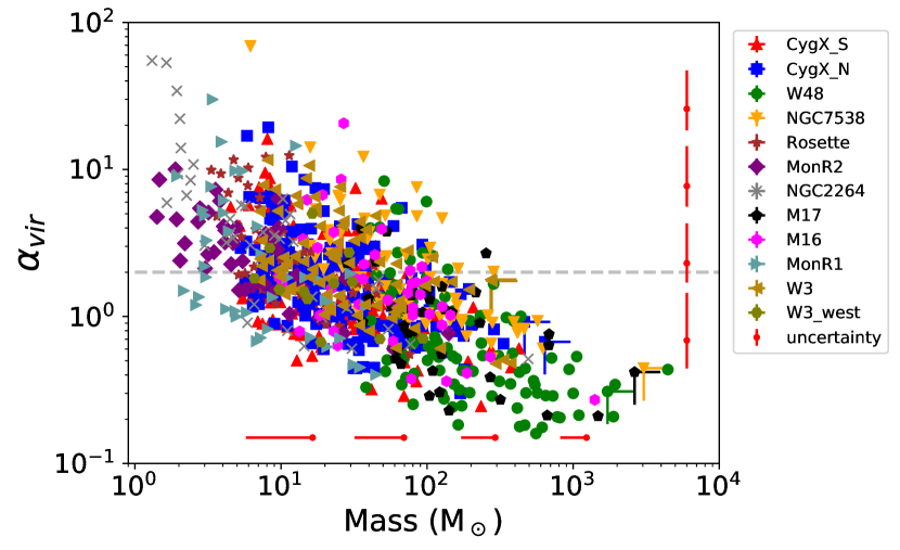
Figure 31: Virial parameter ($\alpha_{vir}$) versus mass for the leaves identified in each region. The dashed line denotes $\alpha_{vir}$ = 2 when assuming a power-law density profile for the structures. Above this line, structures are deemed to be gravitationally unbound in the absence of magnetic fields or external pressure. The red dots with errorbars show the median mass and radius uncertainties in different bins along each axis. All other errorbars show leaves that have mass lower limits due to saturated pixels in the H₂ column density map (see Section 2.3).

Table 4: W3-west NH₃ (1,1) Leaves Catalog 1

ID	RA	decl.	PA	$\sigma_{major}$	$\sigma_{minor}$	$R_{eff}$	$M_{obs}$	$M_{clip}$	$T_{K}$	$\sigma_{NH_{3}}$	$V_{LSR,NH_{3}}$	log($N_{para-NH_{3}}$)	log($N_{H_{2}}$)
	(deg)	(deg)	(deg)	($\arcsec$)	($\arcsec$)	(pc)	(M⊙)	(M⊙)	(K)	(km s-1)	(km s-1)	(cm-2)	(cm-2)
0	34.9844	61.0428	166	16.6	9.9	0.27 ${}^{+0.07}_{-0.06}$	18.7	3.8	10.9 $\pm$ 2.4	0.13 $\pm$ 0.02	-15.2	13.7	21.4
1	35.4211	61.0938	167	30.7	12.8	0.41 ${}^{+0.27}_{-0.15}$	93.7	37.2	13.1 $\pm$ 1.7	0.36 $\pm$ 0.04	-49.9	13.9	21.5
2	35.3625	61.0890	180	14.6	10.8	0.24 ${}^{+0.08}_{-0.13}$	23.0	4.2	13.0 $\pm$ 2.4	0.36 $\pm$ 0.05	-49.7	14.1	21.5
3	35.6144	61.0918	101	14.5	7.0	0.17 ${}^{+0.09}_{-0.12}$	6.6	1.5	10.2 $\pm$ 3.6	0.21 $\pm$ 0.04	-49.4	13.6	21.3
4	35.2711	61.1001	196	22.1	12.1	0.33 ${}^{+0.22}_{-0.19}$	47.5	14.3	12.2 $\pm$ 2.5	0.27 $\pm$ 0.04	-49.7	14.0	21.5
5	35.5964	61.1042	90	10.8	6.2	0.16 ${}^{+0.05}_{-0.01}$	8.4	1.3	16.5 $\pm$ 3.0	0.34 $\pm$ 0.06	-50.1	13.4	21.3
6	35.4752	61.1064	152	17.8	10.6	0.27 ${}^{+0.07}_{-0.07}$	29.2	7.2	15.4 $\pm$ 2.6	0.52 $\pm$ 0.07	-50.0	13.8	21.5
7	35.2490	61.1213	63	10.2	8.1	0.17 ${}^{+0.02}_{-0.03}$	9.7	1.6	13.0 $\pm$ 3.9	0.23 $\pm$ 0.06	-49.6	13.9	21.5
8	35.2099	61.1515	68	13.8	9.7	0.23 ${}^{+0.08}_{-0.03}$	14.4	2.3	12.3 $\pm$ 3.2	0.25 $\pm$ 0.05	-48.8	13.1	21.5
9	35.1733	61.1655	155	14.4	8.2	0.21 ${}^{+0.1}_{-0.03}$	15.2	4.8	12.8 $\pm$ 2.8	0.25 $\pm$ 0.05	-48.7	13.8	21.5
10	35.2731	61.4578	86	16.1	9.5	0.22 ${}^{+0.13}_{-0.04}$	30.8	7.6	14.8 $\pm$ 2.5	0.46 $\pm$ 0.06	-51.0	13.8	21.5
11	35.2470	61.4522	191	13.4	9.0	0.18 ${}^{+0.08}_{-0.08}$	16.4	1.2	12.6 $\pm$ 3.5	0.67 $\pm$ 0.11	-51.4	14.0	21.5

Columns show the following values for each leaf: (1) Leaf ID, (2-3) Mean Right Ascension and Declination in J2000 coordinates, (4) Position angle of the major axis, measured in degrees counterclockwise from the west on sky, (5-6) Major and minor axis measured by astrodendro based on the intensity weighted second moment in the direction of greatest elongation, (7) Effective radius defined as $R_{eff}=(A/\pi)^{1/2}$, where $A$ is the area of all pixels in the leaf’s mask on the position-position plane, (8) Observed mass of leaf from the sum of its H₂ column density, (9) lower limit mass of leaf calculated using the “clipping” technique (see text), (10-13) Average kinetic gas temperature, velocity dispersion, NH₃ (1,1) centroid velocity, and para-NH₃ column density for leaf, all weighted by the NH₃ (1,1) integrated intensity map, along with their 1-sigma uncertainties, (14) Median H₂ column density for leaf measured from the spatially-filtered column density map and used as $N$ in Equation 7. Both column densities are shown in logarithmic scale. Similar tables for all other KEYSTONE regions are available online. Although the intensity-weighted major and minor axes of some sources are less than the $32\arcsec$ beam size of the observations, our culling criteria ensure that their total areas when considering all their associated pixels are larger than $32\arcsec$.

Table 5: W3-west NH₃ (1,1) Leaves Catalog 2

ID	$\alpha_{vir}$	$M_{vir}$	$\sigma_{nt}$	log$|\Omega_{G}|$	log$\Omega_{K}$	log$|\Omega_{Pw}|$	log$|\Omega_{Pt}|$	on-filament	hub	$N_{proto}$	Bad N(H2) Pixels
		(M⊙)	(km s-1)	(erg)	(erg)	(erg)	(erg)
0	0.67	12.6	0.10	43.8	43.4	44.2	NaN	True	False	0	0
1	0.71	66.3	0.36	45.0	44.7	44.8	NaN	True	False	4	0
2	1.68	38.6	0.36	44.1	44.1	44.1	NaN	True	False	1	0
3	1.82	12.0	0.20	43.1	43.2	43.5	NaN	True	False	0	0
4	0.70	33.3	0.26	44.5	44.2	44.5	NaN	True	False	2	0
5	2.92	24.5	0.33	43.4	43.6	43.5	NaN	True	False	1	0
6	2.72	79.6	0.51	44.2	44.4	44.3	NaN	True	False	0	0
7	1.53	14.9	0.21	43.4	43.4	43.7	NaN	True	False	1	0
8	1.47	21.2	0.24	43.7	43.6	44.0	NaN	True	False	0	0
9	1.32	20.0	0.24	43.8	43.7	43.9	NaN	True	False	1	0
10	1.72	52.9	0.45	44.3	44.4	44.0	NaN	True	False	1	0
11	5.01	82.0	0.67	43.9	44.4	43.8	NaN	True	False	0	0

Columns show the following values for each leaf: (1) Leaf ID, (2) virial parameter defined as M_vir/M_obs, (3) virial mass calculated using Equation 1, (4) non-thermal component of the velocity dispersion, (5) gravitational energy density calculated using Equation 5, (6) kinetic energy density calculated using Equation 6, (7) cloud weight pressure energy density calculated using Equation 4, (8) turbulent pressure energy density calculated using Equation 4, with NaN representing a lack of C¹⁸O data for that leaf, (9-10) whether or not the leaf is on-filament or a hub, (11) number of 70 $\mu$m point sources within the leaf’s boundary, (12) fraction of pixels in the leaf that were saturated in the H₂ column density map. Similar tables for all other KEYSTONE regions are available online.

3.6 Identifying filaments and candidate YSOs

Although dendrograms are able to identify the hierarchical parent structures in which leaves are embedded, they are not optimized for isolating the elongated, filamentary structures that are commonly observed in molecular clouds. To understand how the ammonia-identified leaves in this paper relate to surrounding filamentary structures, we employ a dedicated filament extraction algorithm called getfilaments (Men’shchikov, 2013) to identify filaments in each region’s H₂ column density map. The getfilaments algorithm is a multi-scale extraction approach designed to identify filamentary background structures in Herschel maps (e.g., Könyves et al., 2015; Rivera-Ingraham et al., 2016; Marsh et al., 2016; Bresnahan et al., 2018). As such, it performs far better than dendrograms at identifying filaments. getfilaments was run on all the Herschel H₂ column density maps using the standard extraction parameters for the algorithm (see Men’shchikov (2013) for the extensive list of getfilaments parameters). The top left panels in Figures 32-43 display the final filament masks, reconstructed up to spatial scales of 145$\arcsec$.

A leaf that has at least one of its pixels corresponding to at least one pixel in a filament mask is designated “on-filament” and all other leaves are termed “off-filament.” The “on-filament fraction,” i.e., the fraction of leaves in a cloud that are on-filament, is listed in Table 6 and ranges from 0.35 in Cygnus X South to 1.0 in W3-west. For the full sample of 835 leaves with Herschel observations, 454 are on-filament (on-filament fraction of $\sim 54~{}\%$).

To compare the number of star-forming leaves in each KEYSTONE region, we identify young, embedded protostars using the Herschel $70~{}\mu$m maps observed for each cloud. getsources (Men’shchikov et al., 2012), a multi-scale source extraction algorithm designed to identify dense cores and protostars in Herschel observations, was employed to extract point sources at 70 $\mu$m only. We adopt the Herschel Gould Belt Survey selection criteria for candidate young stellar objects (YSOs) described in Section 4.5 of Könyves et al. (2015). The final candidate YSOs are shown as red circles in Figures 32-43. We note that at the distances of the KEYSTONE clouds (0.9 kpc $<d<$ 3.0 kpc), there may be significant incompleteness plus insufficient resolution to separate close sources in the Herschel 70 $\mu$m maps. For some regions, there may also be contamination by photodissociation regions that can appear as 70 $\mu$m point sources. Since we are only using these 70 $\mu$m point sources to indicate which leaves are currently star-forming, rather than using them as a complete catalog of YSOs, the extraction is sufficient for our goals.

We perform a cross-match between the candidate YSO catalogs and leaf catalogs to determine which leaves are protostellar. Leaves with at least one candidate YSO falling within their dendrogram-identified boundary are designated “protostellar.” Conversely, leaves without a candidate YSO are termed “starless.” The protostellar leaf fraction is listed in Table 6 and ranges from 0.17 in MonR1 to 0.58 in W3-west. For the 835 leaves with Herschel observations, 288 are protostellar ($\sim 34~{}\%$).

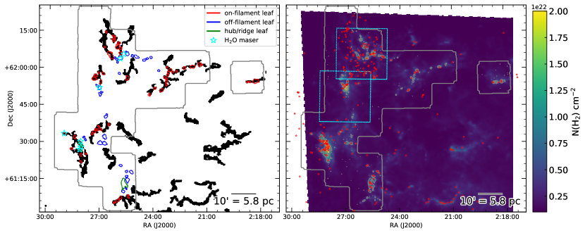
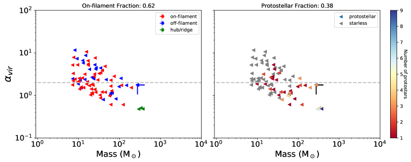
Figure 32: Top Right: Herschel H₂ column density map of W3 with positions of candidate YSOs identified by getsources at 70 $\mu$m overlaid as red dots. The outer grey outline denotes the area mapped by KEYSTONE. The grey contours show NH₃ (1,1) integrated intensity at 1.0 K km s^-1, 3.5 K km s^-1, and 10 K km s^-1. The cyan dotted line outlines the area observed in C¹⁸O $(3-2)$ by the JCMT, which we fit to derive external pressure terms for the subset of leaves falling within those observations (see Section 4.5). Top Left: masks of filaments identified in the Herschel H₂ column density map by getfilaments, reconstructed up to scales of 145$\arcsec$. The positions of our ammonia-identified leaves are overlaid, with red denoting an “on-filament” leaf, blue representing an “off-filament” leaf, and green showing “hubs/ridges” that have uncharacteristically larger masses than the majority of leaves in their respective cloud and tend to be located at filament intersections (see Section 4.1). Cyan stars show the positions of H₂O maser emission. Bottom row: virial parameters versus mass for the protostellar and starless leaves (right) as well as the on-filament, off-filament, and hub sources shown in the top left panel (left). The data point shape in these plots is the same as in Figure 2. Errorbars show leaves that have mass lower limits due to saturated pixels in the H₂ column density map (see Section 2.3).

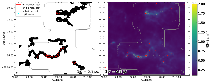
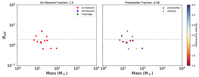
Figure 33: Same as Figure 32 for W3-west.

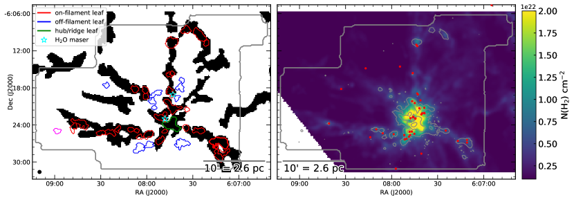
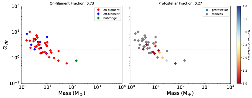
Figure 34: Same as Figure 32 for MonR2. Magenta contours on the left side of the upper left panel denote leaves that were not included in our virial analysis since their masses could not be estimated due to their locations being outside our H₂ column density map boundaries.

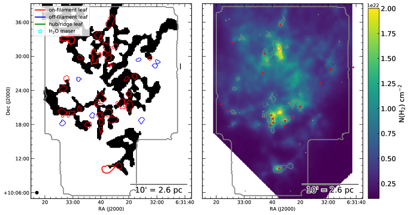
Figure 35: Same as Figure 32 for MonR1.

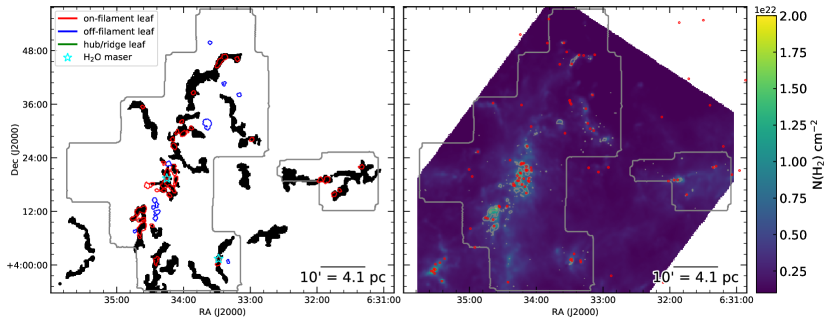
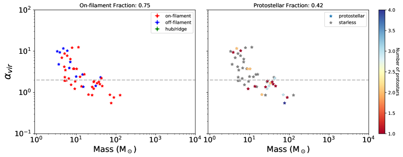
Figure 36: Same as Figure 32 for Rosette.

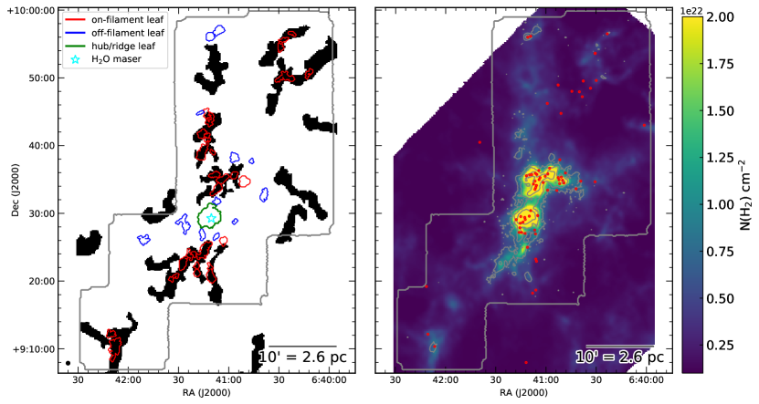
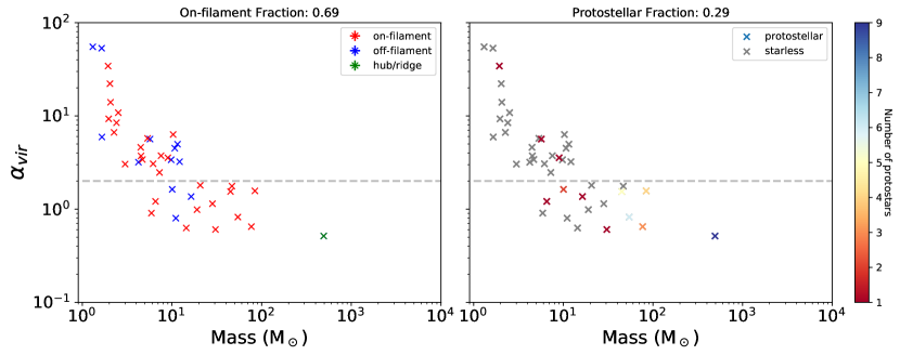
Figure 37: Same as Figure 32 for NGC2264.

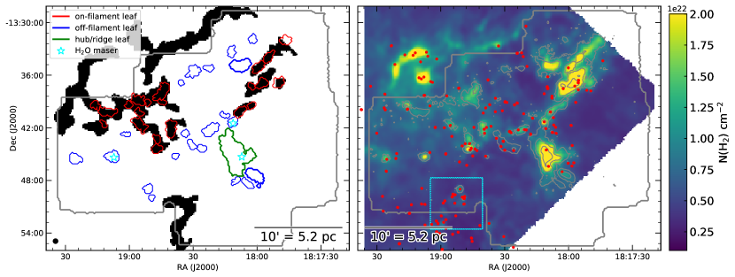
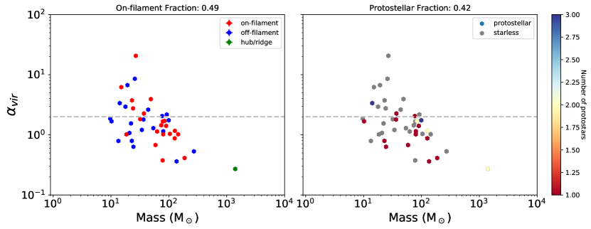
Figure 38: Same as Figure 32 for M16.

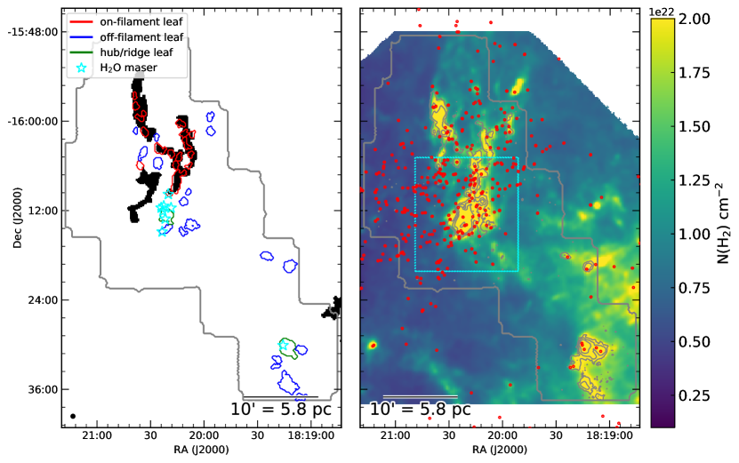
Figure 39: Same as Figure 32 for M17.

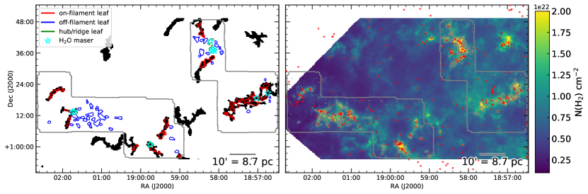
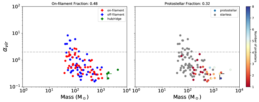
Figure 40: Same as Figure 32 for W48.

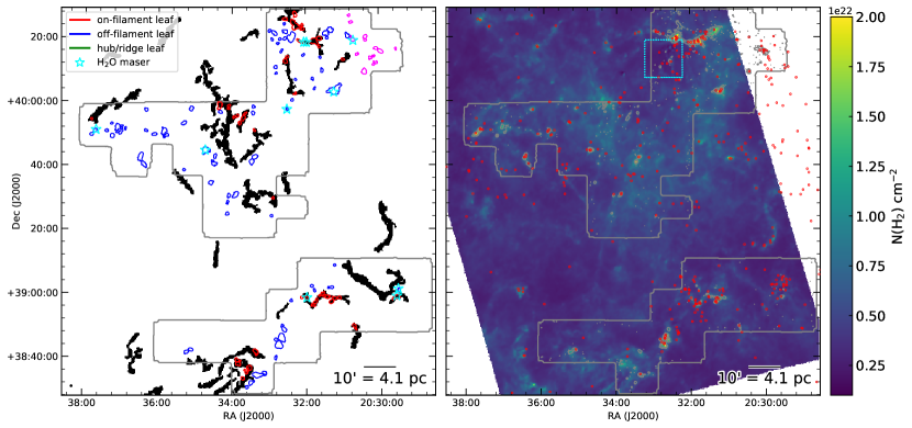
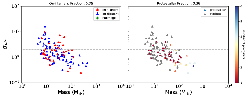
Figure 41: Same as Figure 34 for Cygnus X South.

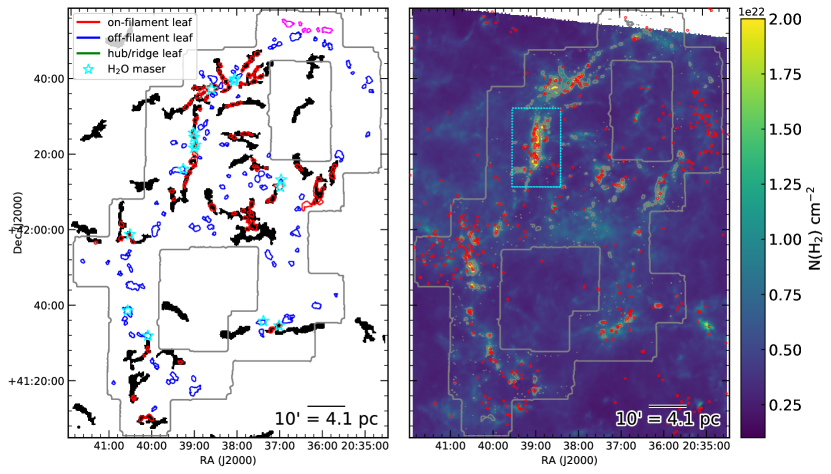
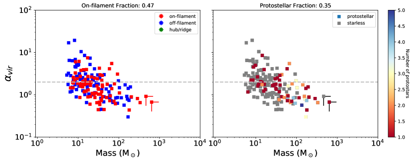
Figure 42: Same as Figure 34 for Cygnus X North.

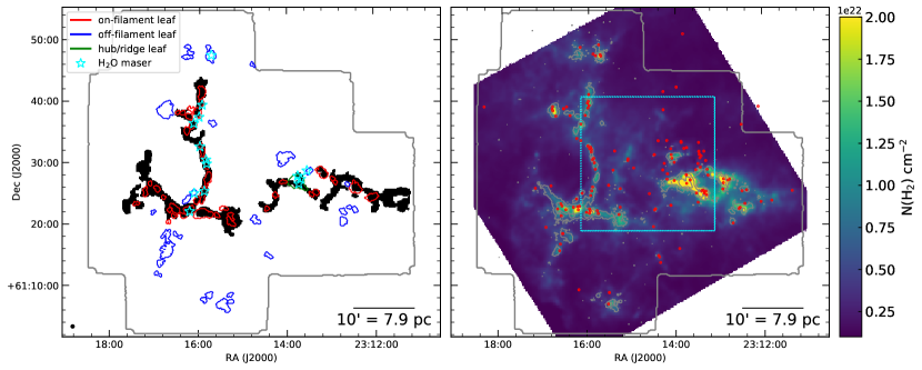
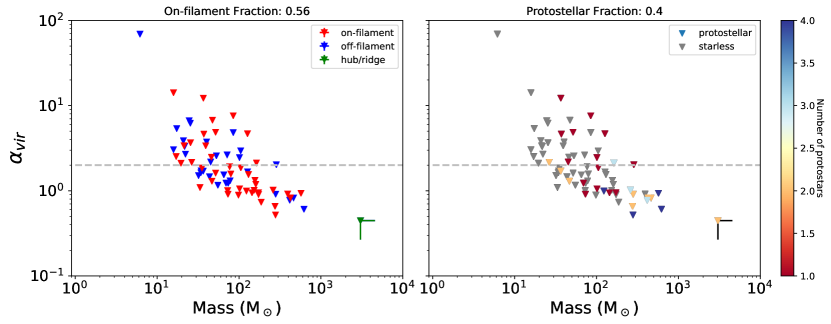
Figure 43: Same as Figure 32 for NGC7538.

3.7 Cloud Population Statistics

To understand the impact environment has upon the star formation in the KEYSTONE clouds, we search for relationships between ten variables of interest: leaf on-filament fraction, “bound” leaf fraction (i.e., the fraction of leaves with $\alpha_{vir}<2$), protostellar leaf fraction, total dense gas mass, total protostar count, total leaf count, dense gas surface mass density, surface protostar density, median cloud kinetic temperature, and cloud distance. The dense gas mass, total protostar count, dense gas surface mass density, and surface protostar density are calculated over the KEYSTONE-mapped boundaries of the cloud where the NH₃ (1,1) integrated intensity is greater than 1.0 K km s^-1. The dense gas mass is defined as the integrated H₂ column density within the NH₃ (1,1) 1.0 K km s^-1 integrated intensity contour, while the total protostar count is defined as the number of candidate YSOs identified by getsources within that same contour. The threshold of NH₃ (1,1) integrated intensity above 1.0 K km s^-1 was chosen since it typically highlights the extent of pixels that were robustly fit during our line-fitting procedure (see, e.g., the lowest NH₃ (1,1) integrated intensity contours in Figures 4-15). Median values of H₂ column density within the NH₃ (1,1) 1.0 K km s^-1 integrated intensity contours are typically around $1\times 10^{22}$ cm^-2, with a minimum of $4.2\times 10^{21}$ cm^-2 measured in W3-west and a maximum of $2.3\times 10^{22}$ cm^-2 measured in M17.

Figure 44 shows the Pearson correlation coefficients for the matrix of ten variables. The Pearson correlation coefficient can range from $-1$ to 1, where $-1$ and 1 signify the data fall on a straight line with a negative or positive correlation, respectively. A Pearson correlation coefficient of zero indicates there is no correlation between the variables. For 12 data points and using the Student’s $t$-distribution to test for statistical significance, the null hypothesis that the data have no relationship is rejected at the $99.5\%$ confidence level when the Pearson correlation coefficient is greater than $\sim|0.71|$. As such, correlations that meet this threshold are outlined by black in Figure 44 and the corresponding scatter plots are shown in Figure 45.

Eight statistically significant correlations were found in the data: 1) decreasing leaf on-filament fraction with increasing dense gas mass, 2) decreasing leaf on-filament fraction with increasing number of protostars, 3) decreasing leaf on-filament fraction with increasing number of leaves, 4) decreasing bound leaf fraction with increasing protostellar surface density, 5) increasing dense gas mass with increasing number of protostars, 6) increasing number of protostars with increasing number of leaves, 7) increasing surface mass density with increasing temperature, and 8) decreasing protostellar surface density with increasing cloud distance.

Since the Pearson correlation coefficient does not take into consideration the uncertainties on each data point, we visualize the scatter of each parameter in Figure 45 by adding errorbars as follows: The lower and upper leaf on-filament fraction errorbars represent the on-filament fractions obtained when using the getfilaments filament masks reconstructed up to spatial scales of $72\arcsec$ and $290\arcsec$, respectively, rather than the $145\arcsec$ scale map. Errorbars for the bound leaf fraction reflect the fractions obtained when assuming the virial parameters for each leaf are at the extremes of their individual uncertainty range. Errorbars for the total protostars, protostellar surface density, and NH₃-leaves represent the $\sqrt{N}$ counting uncertainty. Errorbars for the median kinetic temperature represent the median absolute deviation of each cloud’s $T_{K}$ distribution.

Many of these correlations can be explained with our current understanding of the star formation process. For instance, the positive correlation between dense gas mass and protostars (Panel 5 in Figure 45) is related to the relationship between star formation rate (SFR) and dense gas mass that is well-established (e.g., Gao & Solomon, 2004; Wu et al., 2005, 2010; Lada et al., 2012; Stephens et al., 2016; Burkhart, 2018). Similarly, the correlation we observe between protostars and total ammonia-identified leaves (Panel 6 in Figure 45) is also related to the SFR-Mass relation since the leaves are tracing the dense gas mass in each cloud. Moreover, the negative relationship observed between leaf on-filament fraction and dense gas mass (Panel 1 in Figure 45) may also be loosely related to the SFR-Mass relation. Since the lower mass clouds in our sample tend to have higher leaf on-filament fractions, this trend may suggest that the star formation in those environments is more heavily dependent on filaments creating the high densities required to form ammonia leaves. Clouds with higher dense gas mass, however, can form clumps and stars even when filaments are not present due to their more widespread dense gas. The same argument can be applied to the anti-correlations observed between leaf on-filament fraction versus protostars and ammonia-identified leaves (Panels 2 and 3 in Figure 45). The SFR-Mass relation could also explain the positive relationship between temperature and surface mass density displayed in Panel 7 of Figure 45 since a higher SFR could lead to higher gas temperatures. Panel 7 has the lowest Pearson coefficient absolute value (0.71) of all the relationships shown in Figure 45 and is dominated by two data points, however, which suggests it is not as robust as the other relationships presented.

In addition, the negative trend observed between bound leaf fraction and protostellar surface density (Panel 4 in Figure 45) may be related to the heating and turbulence injected into the cloud by protostars (e.g., Krumholz & McKee, 2008; Hansen et al., 2012; Offner & Chaban, 2017; Offner & Liu, 2018; Cunningham et al., 2018). As the protostellar density increases, the virial parameters of the leaves may increase due to the higher velocity dispersions and temperatures caused by nearby protostellar (or cluster) feedback (e.g., radiation and outflows). Such a scenario is also suggested by the magneto-hydrodynamic simulations of Offner & Chaban (2017), which showed that cores become unbound soon after ($<0.1$ Myr) the onset of protostar formation due to outflow-induced turbulence. Lastly, the negative correlation between protostar surface density and cloud distance shown in Panel 8 is likely related to the larger areas observed for the more distant clouds, which would lower their protostar surface densities. Since protostellar surface density is the only parameter significantly correlated with distance, the distance dependency of the other parameters shown in Figure 44 is likely minimal.

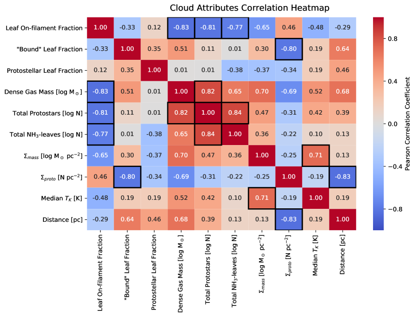
Figure 44: Heatmap of Pearson correlation coefficients for the ten variables of interest examined: leaf on-filament fraction, “bound” leaf fraction (i.e., the fraction of leaves with $\alpha_{vir}<2$), protostellar leaf fraction, total dense gas mass, total protostar count, total leaf count, dense gas surface mass density, surface protostar density, median cloud kinetic temperature, and cloud distance. The colorbar ranges from $-1$ (perfect anti-correlation) to 1 (perfect positive correlation). Panels with a black outline denote statistically significant correlations that are displayed in Figure 45.

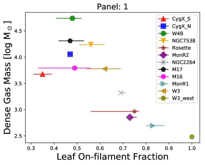
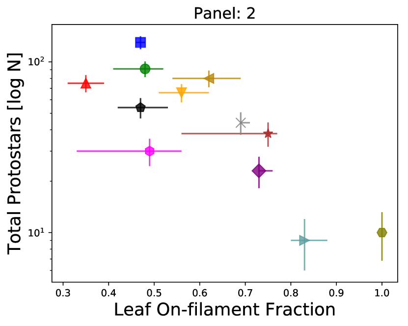
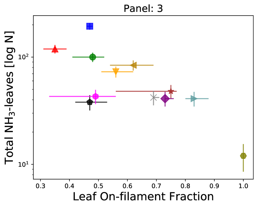
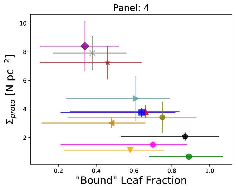
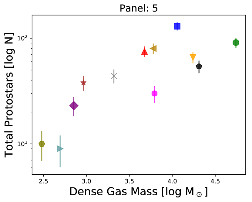
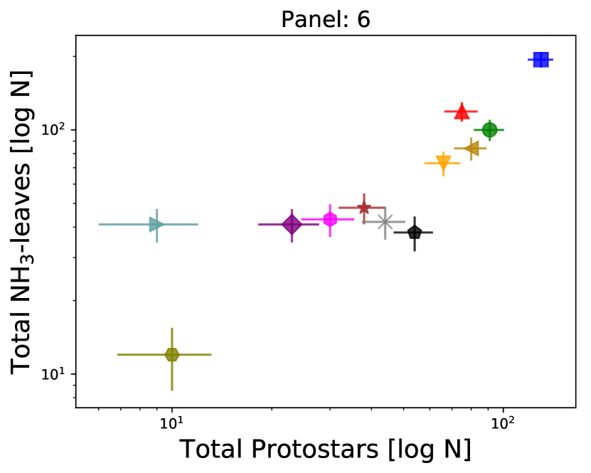
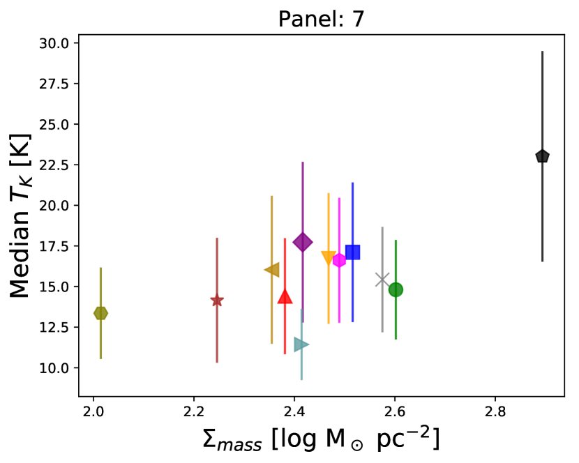
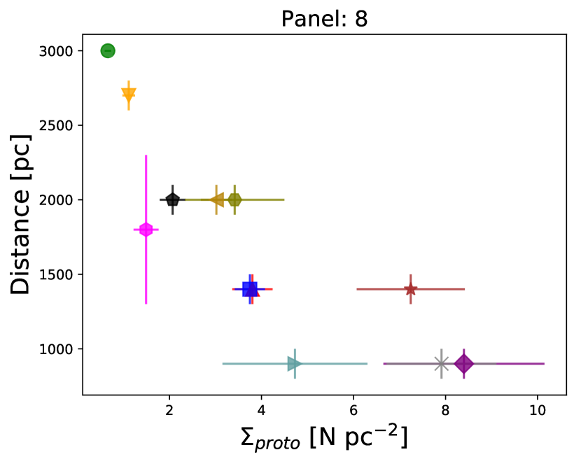
Figure 45: Statistically significant correlations found from Figure 44 when neglecting data errorbars. The dense gas mass, number of protostars, and surface protostar density are calculated within the boundaries of the KEYSTONE-mapped regions in each cloud where NH₃ (1,1) integrated intensity was greater than 1.0 K km s^-1. The errorbars on each data point are calculated as described in Section 3.7.

4 Discussion

4.1 Leaf/Filament Relationship

A relationship between dense cores and filamentary structures in dust continuum observations has been noted in several nearby star-forming environments. Polychroni et al. (2013) show that $67\%$ of the dense cores they identified with CuTEx, a Gaussian fitting and background subtraction source extraction algorithm developed by Molinari et al. (2011), were coincident with filamentary structures in L1641 of Orion A. Using the same filament identification algorithm adopted in this paper, Könyves et al. (2015), Marsh et al. (2016), and Di Francesco et al. (2019, in prep) also found that $75\%$, $40\%$, and $40-80\%$ of starless dense cores in Aquila, Taurus-L1495, and five regions of the Cepheus Flare, respectively, are coincident with filamentary structures. In addition, hydrodynamical simulations of molecular clouds (e.g., Offner et al., 2013) also show a strong correspondence between cores and filamentary structures (Mairs et al., 2014). Although the KEYSTONE clouds analyzed in this paper are located at much farther distances ($0.9-3.0$ kpc) than L1641 (400 pc), Aquila ($250-450$ pc), Taurus-L1641 (140 pc), and Cepheus ($\sim 300$ pc), we find consistent values for the on-filament fraction ($\sim 0.4-1.0$ for KEYSTONE clouds).

Despite the apparent relationship observed between leaves and filaments, we find no significant variations between the virial parameters of the on- and off-filament leaf populations in any of the clouds. For the 454 on-filament leaves, 294 ($\sim 65~{}\%$) have $\alpha_{vir}<2$, which is consistent with the bound fraction for the entire leaf population ($\sim 63~{}\%$). Furthermore, Figure 46 shows that the mass, effective radius, average kinetic temperature, and average velocity dispersion for the on-filament and off-filament leaves are essentially identical. Although the more distant clouds (e.g., W48 and NGC7538) tend to have larger masses and radii than the nearest clouds in our sample (e.g., MonR1, MonR2, and NGC2264; see Appendix A for a discussion of the distance dependency of our results), the similarities between the on-filament and off-filament leaf parameter distributions appear to hold for the individual clouds as well. These similarities indicate that star formation away from filaments might be equally as likely as star formation on filaments in high-mass GMCs since dense gas may be more widespread in those environments. Such a scenario is also suggested by the anti-correlation found between leaf on-filament fraction and dense gas mass discussed in Section 3.7. As dense gas becomes more widespread in high-mass GMCs, the fraction of star formation taking place on filaments may decrease since dense gas is equally as likely to be found away from filaments as it is to be found within filaments.

We also note the existence of a group of ammonia-identified leaves with uncharacteristically larger masses ($10^{2}-10^{3}$ M_⊙) than the majority of leaves in their respective clouds. Deemed “hubs” or “ridges” based on the nomenclature suggested in Myers (2009), these high-mass leaves are shown by the color green in Figures 32-43. The hubs are located at the intersection of multiple filaments (e.g., MonR2, NGC2264, eastern and northern regions in W48) and the ridges are massive filaments (e.g., NGC7538, M16, southern region of W48). Due to their high masses, these structures all have low virial parameters ($\alpha_{vir}=0.2-0.5$) and are likely gravitationally bound or collapsing. As such, the hubs and ridges may be a result of mass build-up at the locations where filaments are transporting mass from other parts of the cloud.

In addition to the hubs and ridges being coincident with filaments, their mass and size indicate they are likely the precursors of massive young stellar objects and stellar clusters. For example, the right panel of Figure 30 shows the Mass-Radius plot for the hub/ridge and non-hub/ridge leaves in relation to the Kauffmann & Pillai (2010) empirically-derived threshold for massive star formation: m(r) $>$ 870 M_⊙ (r/pc)^1.33. The hubs and ridges tend to be above this threshold, indicating that they will likely form high-mass stars. As shown in Figure 46, the hubs and ridges tend to have higher masses (median log($M_{obs}$) = $3.2\pm 0.5$), larger radii (median $R_{eff}$ = $0.7\pm 0.3$), warmer temperatures (median $T_{K,avg}$ = $19.5\pm 5.1$), and larger velocity dispersions (median $\sigma=0.7\pm 0.1$) than the starless leaf population. Instead, the hub and ridge masses, radii, and virial parameters are more similar to the massive star-forming clumps identified by Urquhart et al. (2015), highlighting further their propensity to form massive stars. Furthermore, the hubs and ridges tend to align with the positions of H₂O maser emission (identified by eye and shown as cyan stars in Figures 32-43) also detected by KEYSTONE (White et al., in prep.), which is frequently associated with massive young stellar objects. If dense gas hubs and ridges are indeed the current, or future, sites of massive young stellar object and stellar cluster formation, it would explain the high correspondence observed between those objects and filament intersections (e.g., Myers, 2009; Schneider et al., 2012; Hennemann et al., 2012; Li et al., 2016; Motte et al., 2018a).

4.2 Leaf/Protostar Relationship

Figures 32-43 also show the virial parameters of the leaves identified as protostellar and starless in each of the clouds observed by KEYSTONE. In many regions (e.g., MonR1, Rosette, Cygnus X North, MonR2, W48), the protostellar core population clearly has larger masses and lower virial parameters than the starless core population. For the 288 protostellar leaves identified, 229 ($\sim 80~{}\%$) have $\alpha_{vir}<2$. In comparison, 294 of the 547 starless leaves identified ($\sim 54~{}\%$) have $\alpha_{vir}<2$. As shown in Figure 46, the protostellar population’s mass distribution peaks at higher values (Median log(Mass) = 1.8 $\pm$ 0.6 M_⊙) than that of the starless population (Median log(Mass) = 1.3 $\pm$ 0.5 M_⊙), which could explain the lower protostellar virial parameters. In addition, the hubs and ridges identified in the previous section tend to host multiple protostars (see, e.g., NGC7538, NGC2264, W48, W3, M16). In several regions, the hubs and ridges host over six protostars. Since the 70 $\mu$m maps are typically confusion-limited in the hubs and ridges, their protostar counts are likely under-estimated. This attribute highlights the exceptional environment hubs and ridges provide for cluster formation.

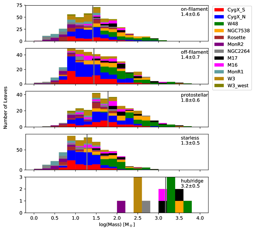
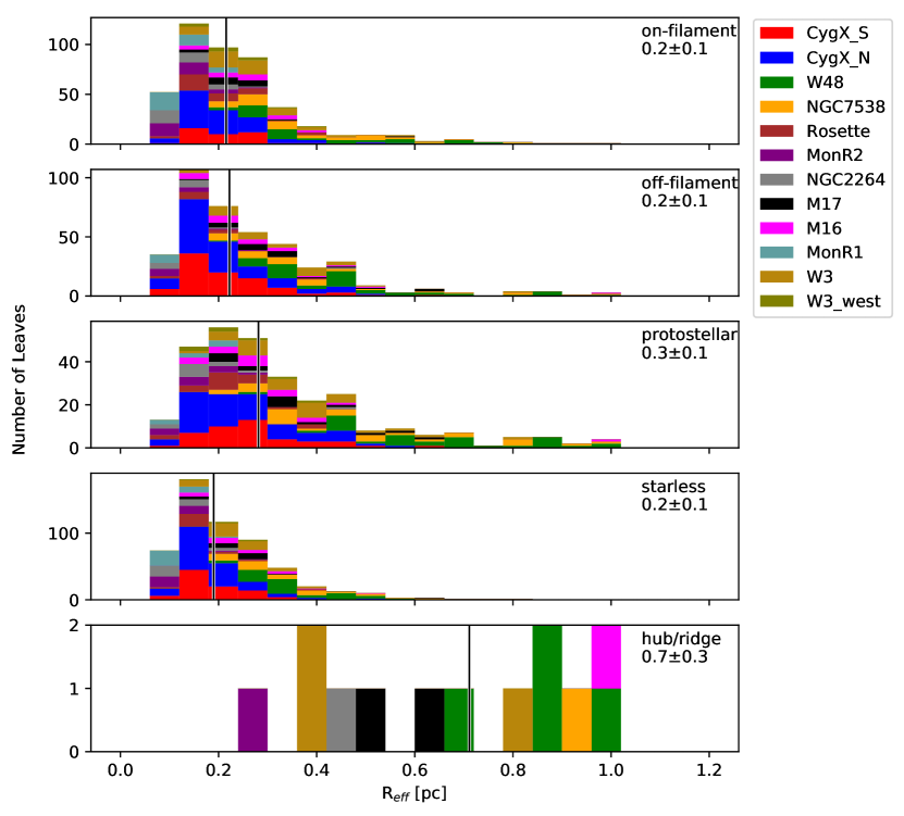
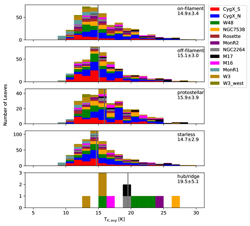
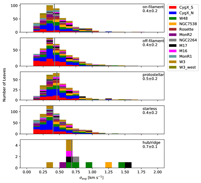
Figure 46: Stacked histograms of mass (upper left), effective radius (upper right), average kinetic temperature (lower left), and average velocity dispersion (lower right) for the leaves identified as on-filament, off-filament, protostellar, starless, and hub/ridge. The median and median absolute deviation of the distributions are shown in the upper right corner of each panel. The black vertical lines show the distribution median.

Table 6: Cloud Statistics

Cloud	Tmed	$\sigma_{med}$	Protostars	Area	Mass	Total Leaves	Filament Leaves	Proto Leaves	Bound Leaves
	K	km s-1		pc2	M⊙		fraction	fraction	fraction
W3	16.0 $\pm$ 4.6	0.5 $\pm$ 0.3	80	26.5	5999	84	0.62	0.38	0.48
W3-west	13.4 $\pm$ 2.8	0.3 $\pm$ 0.1	10	2.9	303	12	1.00	0.58	0.75
MonR2	17.7 $\pm$ 4.9	0.3 $\pm$ 0.2	23	2.7	715	41	0.73	0.27	0.34
MonR1	11.4 $\pm$ 2.2	0.2 $\pm$ 0.2	9	1.9	494	41	0.83	0.17	0.61
Rosette	14.2 $\pm$ 3.8	0.4 $\pm$ 0.1	38	5.2	924	48	0.75	0.42	0.46
NGC2264	15.4 $\pm$ 3.2	0.5 $\pm$ 0.2	44	5.6	2091	42	0.69	0.29	0.38
M16	16.6 $\pm$ 3.8	0.5 $\pm$ 0.2	30	20.1	6207	43	0.49	0.42	0.70
M17	23.0 $\pm$ 6.5	0.7 $\pm$ 0.3	54	26.1	20439	38	0.47	0.42	0.87
W48	14.8 $\pm$ 3.1	0.5 $\pm$ 0.3	91	137.6	55013	100	0.48	0.32	0.89
Cygnus X South	14.4 $\pm$ 3.6	0.4 $\pm$ 0.2	75	19.7	4744	119	0.35	0.36	0.66
Cygnus X North	17.1 $\pm$ 4.3	0.4 $\pm$ 0.2	130	34.7	11383	194	0.47	0.35	0.64
NGC7538	16.7 $\pm$ 4.0	0.6 $\pm$ 0.3	66	59.2	17393	73	0.56	0.40	0.58

Note. — Columns show the following: (1) cloud name, (2-3) median kinetic gas temperature and velocity dispersion for all reliably fit ammonia pixels, (4) number of protostars identified where NH₃ (1,1) integrated intensity is greater than 1 K km s^-1, (5) area of map where NH₃ (1,1) integrated intensity is greater than 1 K km s^-1, (6) total mass where NH₃ (1,1) integrated intensity is greater than 1 K km s^-1, (7) total number of ammonia leaves identified in cloud, (8) fraction of total leaves that are on-filament, (9) fraction of total leaves that are protostellar, (10) fraction of total leaves that are bound ($\alpha_{vir}<2$).

Table 7: Leaf Population Statistics

Leaf Statistic	Fraction
Bound	523 of 835 ($\sim 63\%$)
Starless	547 of 835 ($\sim 66\%$)
Protostellar	288 of 835 ($\sim 34\%$)
On-filament	454 of 835 ($\sim 54\%$)
Bound Starless	294 of 547 ($\sim 54\%$)
Bound Protostellar	229 of 288 ($\sim 80\%$)
Bound On-filament	294 of 454 ($\sim 65\%$)
Sub-virial (cloud weight pressure)	573 of 835 ($\sim 69\%$)

Note. —  Leaf population statistics quoted throughout the paper. All fractions are in relation to the sample of leaves with mass estimates.

4.3 Virial Stability in Low- and High-Mass Star-Forming Regions

Our final sample of 835 ammonia-identified leaves, for which virial parameters have been measured in a consistent manner, forms one of the largest current samples of dense gas structure virial parameters in high-mass star-forming regions. While many studies have derived virial parameters for single molecular clouds or sub-samples of clumps/cores (e.g., Dunham et al., 2010; Schneider et al., 2010a; Urquhart et al., 2011; Tan et al., 2013; Li et al., 2013; Urquhart et al., 2015; Friesen et al., 2016; Kirk et al., 2017; Billington et al., 2019), few have viewed virial stability across many clouds. Wienen et al. (2012) observed ammonia emission from a sample of 862 clumps in the inner Galactic disk, but only $\sim 300$ of those had known distance measurements required to estimate masses and virial parameters. Similarly, Kauffmann et al. (2013) compiled a catalog of 1325 virial parameter estimates from previously published catalogs of sources in both high- and low-mass star-forming regions. The Kauffmann et al. (2013) catalog, however, featured virial parameters that had been measured using a variety of molecular tracers (¹³CO, NH₃, N₂D⁺), mass estimation methods (dust continuum and NIR extinction), and probed varying scales (clouds, clumps, and cores). Nevertheless, we can usefully compare the Kauffmann et al. (2013) catalog to our data since it deals primarily with high-mass star-forming regions, uses the same formulation for source effective radius, and uses dust continuum emission to derive the masses for most sources.

Overall, our virial parameters are consistent with those found for the high-mass cores, clumps, and clouds included in the Kauffmann et al. (2013) compilation, which included the clumps observed by Wienen et al. (2012). $\alpha_{vir}$ ranges from $\sim 10^{-1}$ to $10^{2}$ and roughly half of the sources fall below the $\alpha_{vir}$=2 threshold for both the Kauffmann et al. (2013) sources and those presented in this paper. This result is in contrast to the virial analyses of Friesen et al. (2016) in Serpens South and Keown et al. (2017) in Cepheus-L1251, which found that nearly all their ammonia-identified leaves had $\alpha_{vir}<2$. Serpens South and Cepheus-L1251 are closer ($d\sim 250-450$ pc and 300 pc, respectively) than the clouds observed by KEYSTONE and are thus probing smaller scale structures, which may explain the higher rate of gravitationally bound leaves in those papers. These results are supported by those of Ohashi et al. (2016) and Chen et al. (2019b), which used ALMA observations of infrared dark clouds to show that $\alpha_{vir}$ decreases with decreasing spatial scales from filaments to clumps to cores, and may be showing that gravity is more important in the stability of structures at small scales. Alternatively, the KEYSTONE observations may indicate that ammonia is more widespread throughout GMCs than it is in low-mass clouds, producing detectable ammonia emission in both bound and unbound sources. Such a scenario is supported by the observations of Henshaw et al. (2013), which found N₂H⁺ ($1-0$) to be more extended in the infrared dark cloud G035.39-00.33 than in low-mass star-forming environments.

Observations of more distant cloud clumps ($\sim 2-11$ kpc) by the Bolocam Galactic Plane Survey (BGPS; Rosolowsky et al., 2010; Ginsburg et al., 2013), which mapped 1.1 mm dust continuum emission across the Galactic plane, have also indicated low virial parameters ($\alpha_{vir}<2$) for clumps. For instance, Svoboda et al. (2016) combined NH₃ observations with BGPS clump detections to calculate virial parameters for 1640 clumps and found that $76\%$ of starless candidates and $86\%$ of protostellar candidates had $\alpha_{vir}<2$. Similarly, Dunham et al. (2011) found that a separate sample of 456 BGPS clumps had a median $\alpha_{vir}=0.74$. We note, however, that the NH₃ observations used for those analyses were targeted follow-ups to previously identified clumps in the BGPS data. Thus, they may not be tracing the faint NH₃ emission probed by KEYSTONE and included in our leaf catalog. These low brightness NH₃ sources comprise the lower mass leaves in our sample that have $\alpha_{vir}>2$ and may be the reason we detect unbound sources that are lacking in the BGPS data.

A similar selection bias for high brightness sources is likely also impacting clump virial analyses using Herschel Hi-GAL (Molinari et al., 2010) and APEX Telescope ATLASGAL (Schuller et al., 2009) observations. For example, Merello et al. (2019) combined Hi-GAL clump detections with NH₃ catalogs to derive virial parameters for 1068 clumps at distances typically between $\sim 2$ kpc and $\sim 15$ kpc. $72\%$ of the 1068 clumps had $0.1<\alpha_{vir}<1$, with a median $\alpha_{vir}$ of 0.3. A similar virial analysis of 213 Hi-GAL clumps by Traficante et al. (2018) found that $76\%$ have $\alpha_{vir}<1$. Using a sample of 1244 ATLASGAL clump detections with masses much larger (typically $>10^{3}M_{\odot}$) than the leaves presented in this paper, Contreras et al. (2017) found a median $\alpha_{vir}$ of 1.1. Since these analyses rely on clump catalogs identified by dust continuum observations, however, they likely exclude the faint NH₃ sources detected by KEYSTONE.

4.4 Cloud Weight Pressure

Although the virial analysis presented in Section 3.5 compares the gravitational energy of the ammonia-identified leaves with their kinetic energy, it excludes the possible influence of external pressure applied by the leaves’ surroundings (Field et al., 2011). For instance, the weight of the molecular cloud in which the leaves are embedded can contribute to their confinement (e.g., Pattle et al., 2015, 2017; Kirk et al., 2017). Here, we add the cloud weight pressure energy density ($\Omega_{Pw}$) to the virial equation using the technique described in Keown et al. (2017) and Kirk et al. (2017). The three energy densities in the virial equation considered in our analysis are given by the following expressions:

$$\Omega_{Pw}=-4\pi P_{w}R^{3}$$ (4)

$$\Omega_{G}=\frac{-1}{2\sqrt{\pi}}\frac{GM^{2}}{R}$$ (5)

$$\Omega_{K}=\frac{3}{2}M\sigma^{2}$$ (6)

where $M$ is the observed structure mass, $R$ is the effective radius, $G$ is the gravitational constant, $\sigma^{2}$ is the same as Equation 3, and $P_{w}$ is cloud weight pressure:

$$P_{w}=\pi G\bar{N}N(\mu_{H}m_{H})^{2}$$ (7)

where $\bar{N}$ is the mean cloud column density and $N$ is the column density at the structure (e.g., McKee, 1989; Kirk et al., 2006, 2017). Both $\bar{N}$ and $N$ are measured from a spatially filtered column density map to determine the cloud’s mass contribution from large-scale structures. Following other recent virial analyses incorporating turbulent pressure (Kirk et al., 2017; Keown et al., 2017; Kerr et al., 2019), the a trous transform is used to filter spatially each column density map to spatial scales larger than 2ⁿ pixels, where we have chosen $n$=4 or 16 pixels for all regions. Figure 47 shows an example spatially filtered column density map for NGC 7538, where 16 pixels is equivalent to $\sim 96\arcsec$ or $\sim 1.3$ pc. $\bar{N}$ is calculated as the mean of the spatially filtered column density map, while $N$ represents the mean spatially filtered column density within each leaf’s dendrogram-identified boundary.

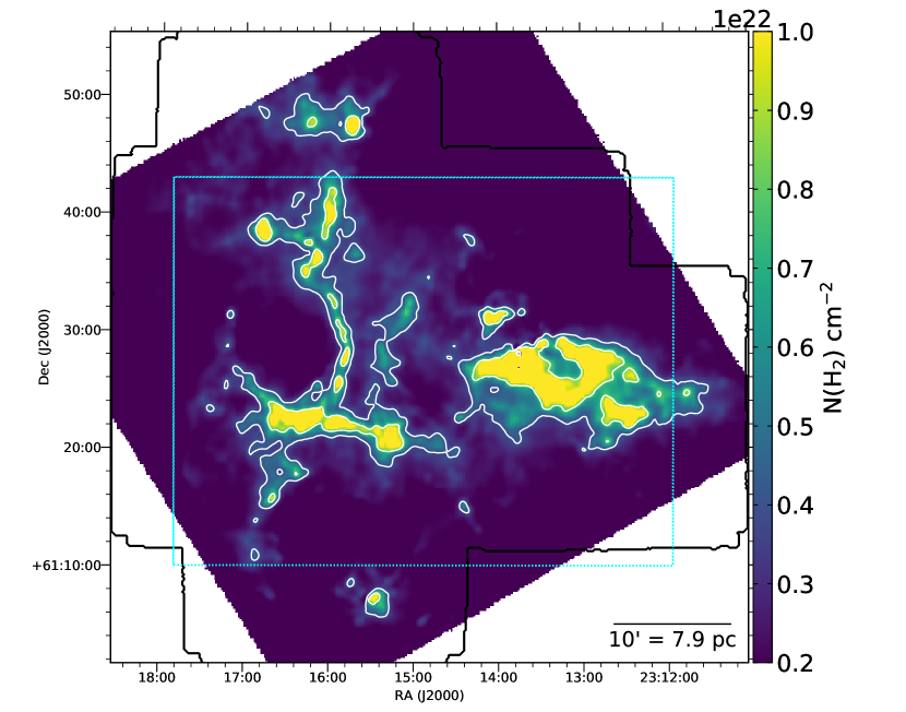
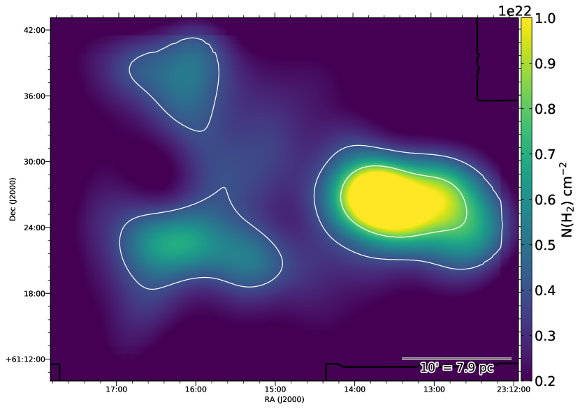
Figure 47: Left: H₂ column density map of NGC7538 with white contours at $4\times 10^{21}$ cm^-2 and $8\times 10^{21}$ cm^-2. Black outlines the extent of the KEYSTONE mapping of the region. Right: Spatially filtered H₂ column density map over the cyan dotted area overlaid in the left panel. The map includes spatial scales larger than 16 pixels, which is equivalent to $\sim 96\arcsec$ or $\sim 1.3$ pc at the distance of NGC7538.

Although we have chosen a single scale for the spatial filtering, a recent virial analysis by Kerr et al. (2019) investigated the impact that varying this scale has upon the cloud weight pressure term. In their analysis of L1688, B18, and NGC1333, Kerr et al. find that increasing or decreasing the spatial filtering scale by a factor of two results in less than a factor of two difference in the average $P_{w}$ values for those clouds. As shown below, such a factor is not enough to change our overall conclusions about the virial stability of the observed structures.

The left panel of Figure 48 shows the balance between cloud weight pressure ($\Omega_{Pw}$), kinetic energy ($\Omega_{K}$), and gravitational potential energy ($\Omega_{G}$) for the 835 leaves with mass estimates. Leaves to the right of the vertical dotted line are deemed “sub-virial” since their gravitational potential and external pressure are enough to overcome their internal kinetic energy in the absence of magnetic fields. Leaves to the left of the vertical line are “super-virial” since they are not bound by their gravitational and external pressure energy densities. Below the horizontal dotted line are “pressure-dominated” sources that have a higher external pressure energy density than their gravitational energy density. Conversely, “gravity-dominated” sources lie above the horizontal line.

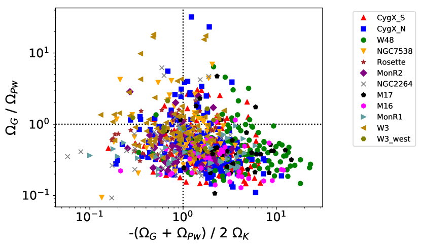
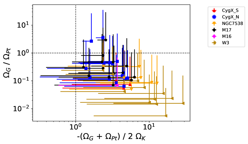
Figure 48: Left: Virial plane for all ammonia-identified leaves displayed in Figure 31 showing the balance between three energy densities in the virial equation: Gravitational ($\Omega_{G}$), Cloud Weight Pressure ($\Omega_{Pw}$), and Kinetic ($\Omega_{K}$). Sources to the right of the vertical line are sub-virial, while sources to the left are super-virial. Sources above the horizontal line are gravitationally-dominated, while sources below the line are pressure-dominated. Right: Virial plane using instead the Turbulent Pressure energy density ($\Omega_{Pt}$) for all ammonia-identified leaves with reliable C¹⁸O $(3-2)$ velocity dispersion measurements. The data points are calculated using the critical density ($3\times 10^{4}$ cm^-3) of C¹⁸O ($3-2$) as the volume density traced by its emission. The errorbars show where the source would fall on the plot if the density traced by the C¹⁸O were a factor of ten lower ($3\times 10^{3}$ cm^-3).

As previous virial analyses in nearby low-mass star-forming regions have shown (Pattle et al., 2015, 2017; Kirk et al., 2017; Keown et al., 2017; Chen et al., 2019a; Kerr et al., 2019), most of the leaves are sub-virial and pressure-dominated. In particular, Kerr et al. (2019) showed that 79 of 134 ($\sim 59\%$) of the cores in their combined sample from the NGC1333, L1688, and B18 clouds were sub-virial when considering both cloud weight pressure and turbulent pressure. Similarly, we find that $\sim 69\%$ of the leaves presented in this paper are deemed sub-virial when considering only the cloud weight pressure in the pressure energy density. This implies that the larger H₂ column densities and total cloud masses observed for GMCs are sufficient to create virially bound structures without the necessity of large levels of turbulent pressure that appear to be required in low-mass star-forming environments (see Section 4.5 below for a discussion of turbulent pressure).

Although many of the structures are pressure-dominated, the large surrounding reservoirs of dense gas in GMCs may facilitate their evolution into the gravitationally-dominated regime. For instance, some recent simulations have shown that even though dense cores may appear as pressure-confined and stable structures at various stages in their evolution, they are still likely to be gaining mass by accreting material from their surroundings and will eventually undergo gravitational collapse (e.g., “global hierarchical collapse,” Naranjo-Romero et al., 2015; Vázquez-Semadeni et al., 2017; Ballesteros-Paredes et al., 2018; Vázquez-Semadeni et al., 2019). As such, the observed pressure-dominated state of our ammonia-identified leaves may be a common stage in their evolution from dense gas structures to protostars and clusters. Furthermore, the dearth of structures in the sub-virial and gravitationally-dominated regime may indicate that clumps spend the majority of their time being pressure-dominated, with a quick transition to being gravitationally-dominated and subsequently collapsing to form protostars.

4.5 Turbulent Pressure

In addition to cloud weight, pressure due to cloud-scale turbulence may have a significant impact on the virial stability of dense cores (e.g., Kerr et al., 2019; Pattle et al., 2015, 2017; Kirk et al., 2017; Keown et al., 2017; Chen et al., 2019a). Here, we calculate the turbulent pressure energy density ($\Omega_{Pt}$) for a subset of our ammonia-identified leaves following the method described by Keown et al. (2017) (see also Pattle et al. (2017) and Kirk et al. (2017) for detailed discussions of turbulent pressure). $\Omega_{Pt}$ is calculated from Equation 4, with P_w being replaced with P_t given by:

$$P_{T}=\mu_{H}m_{H}\times\rho_{C^{18}O}\times\sigma^{2}_{C^{18}O}~{},$$ (8)

where $\sigma_{C^{18}O}$ is the velocity dispersion measured from C¹⁸O $(3-2)$, a moderate density tracer, and $\rho_{C^{18}O}$ is the volume density at which the C¹⁸O $(3-2)$ emission originates. Here, we assume the C¹⁸O $(3-2)$ emission is tracing a volume density of $3\times 10^{4}$ cm^-3, which is the critical density ($n_{cr}(u-l)=A_{ul}/\gamma_{ul}$, where $A_{ul}$ is the Einstein A coefficient and $\gamma_{ul}$ is the collisional rate coefficient for collisions with H₂) of C¹⁸O $(3-2)$ at 20 K (calculated using collisional rate coefficients accessed from the Leiden Atomic and Molecular Database, Schöier et al., 2005).

Six of the eleven KEYSTONE regions were found to have partial JCMT observations of C¹⁸O $(3-2)$ (see Section 2.4 for a discussion of these data and our reduction techniques). A Gaussian model with three free parameters (peak brightness temperature, centroid velocity, and velocity dispersion) was fit to all pixels in the C¹⁸O $(3-2)$ data cubes with SNR $>$ 6 using the non-linear least squares curve-fitting method in the scipy.optimize.curvefit Python package. SNR is measured from the ratio of the peak brightness temperature in each spectra to the standard deviation of the off-line spectral channels. The conservative cutoff of SNR $>$ 6 was chosen to remove low SNR spectra from consideration since they often have higher uncertainties in the fitted parameters. The initial parameter guesses of each fit are based on the brightness and velocity of the peak brightness channel, with a set guess of 1.5 km s^-1 for the velocity dispersion. After the line fitting, pixels must meet the following criteria to be included in our final parameter maps:

1. $\sigma>$ 0.05 km s^-1 (below 0.05 km s^-1 is unrealistic since our channel width is only $\sim$ 0.11 km s^-1;

2. $T_{peak,err}<$ 1 K;

3. $\sigma_{err}<$ 0.5 km s^-1;

4. $V_{LSR,err}<$ 0.75 km s^-1.

The final parameter maps for the velocity dispersion, $\sigma_{C18O}$, are shown in Figures 49-50. The 52 leaves with at least one reliably fit C¹⁸O $(3-2)$ pixel are shown by red contours in Figures 49-50. The median value of $\sigma_{C18O}$ is calculated within the boundaries of each leaf and converted into a turbulent pressure using Equations 5 and 9. Although most of the C¹⁸O $(3-2)$ spectra are well-characterized by a single Gaussian, some do show wings that may be due to outflows or multiple velocity components along the line of sight. These areas can be seen in the velocity dispersion maps as sharp increases in $\sigma_{C18O}$. Since most of the leaves do not overlap with these sharp transitions, our single Gaussian fit is likely sufficient for our velocity dispersion estimates.

The right panel of Figure 48 shows the virial plane for structures with C¹⁸O $(3-2)$ measurements when using $\Omega_{Pt}$ as the pressure term in the virial equation. All of these structures fall within the pressure-dominated, sub-virial quadrant. The ratio of $\Omega_{Pt}$/$\Omega_{Pw}$ for these structures ranges from $\sim 1$ to $\sim 200$, with a median of $\sim 7$. This would suggest that cloud-scale turbulence or global collapse, rather than cloud weight, is the dominant contributor to the pressure term in the virial equation for these ammonia-identified leaves.

Since the turbulent pressure calculation is sensitive to the assumed value of $\rho_{C^{18}O}$, we also calculate $P_{T}$ using a factor of ten lower value ($3\times 10^{3}$ cm^-3) for $\rho_{C^{18}O}$ and show the difference as errorbars in Figure 48. This lower density is more characteristic of the effective excitation density of C¹⁸O $(3-2)$, which is often 1-2 orders of magnitude lower than critical densities (Shirley, 2015). Under this assumption, the ratio of $\Omega_{Pt}$/$\Omega_{Pw}$ correspondingly drops by a factor of ten, with a range from $\sim 0.1$ to $\sim 20$ and a median of $\sim 0.7$. In contrast to the scenario using the higher $\rho_{C^{18}O}$ assumption, this new estimation would suggest that cloud weight is dominant over turbulent pressure.

Several recent virial analyses of nearby star-forming regions such as Ophiuchus, B18, and NGC1333 have shown that turbulent pressure tends to be larger than cloud weight pressure (e.g., Kerr et al., 2019; Pattle et al., 2015). Conversely, cloud weight pressure appears to be larger than turbulent pressure in Orion A (Kirk et al., 2017). We note, however, that these analyses included turbulent pressure measurements across entire clouds. This approach is in contrast to the analysis we present here, which has turbulent pressure measurements for only a small subset of leaves that are generally concentrated on the most active star formation sites in each cloud observed (e.g., DR21 in Cygnus X, W3(OH) and W3 Main in W3, and M17SW in M17) and tend to qualify as hubs or ridges. As such, this biased sample cannot be used to draw generalizations for the full ammonia-identified leaf catalog presented in this paper. Instead, widespread C¹⁸O mapping across the KEYSTONE clouds is required to investigate further the role of turbulent pressure on cloud structure and core dynamics.

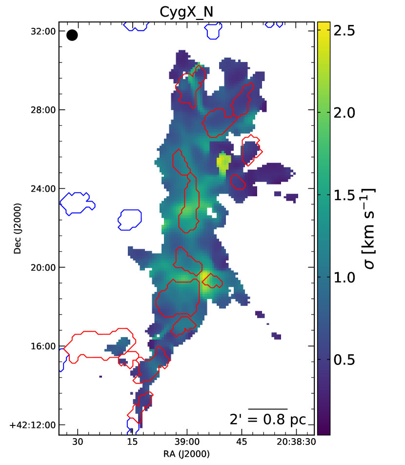
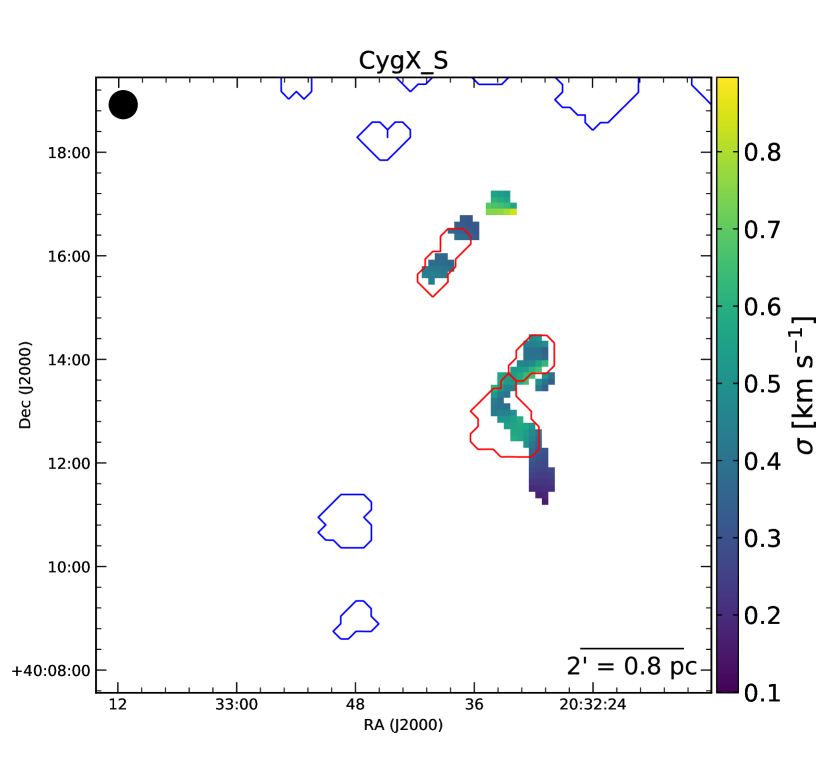
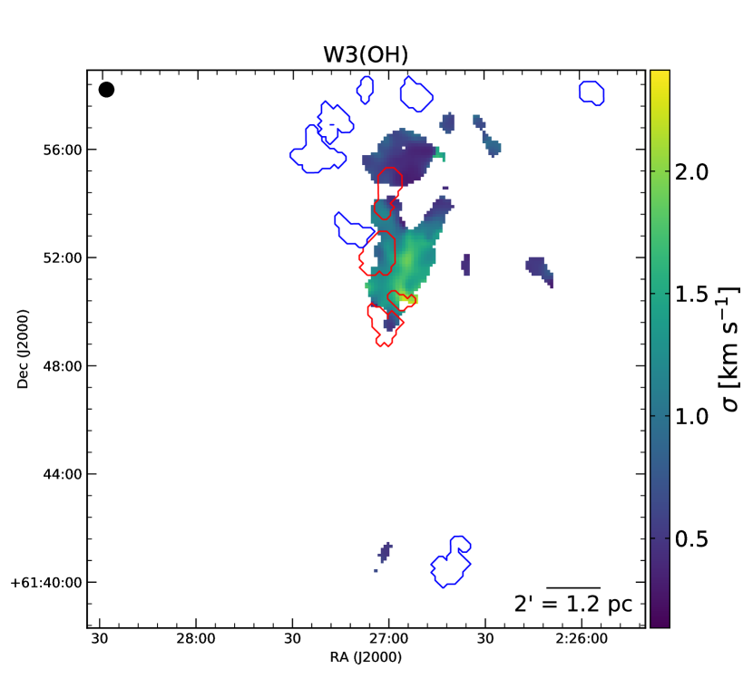
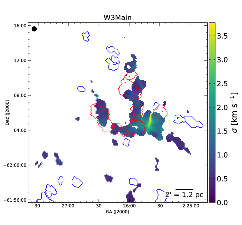
Figure 49: C¹⁸O $(3-2)$ velocity dispersion measured from Gaussian fits to JCMT observations of DR21 in Cygnus X North (top left), G79.34 in Cygnus X South (top right), W3(OH) (bottom left), and W3-Main (bottom right). Red contours denote ammonia-identified leaves that have at least one reliably fit C¹⁸O $(3-2)$ pixel and were included in our turbulent pressure virial analysis. Blue contours show all other ammonia-identified leaves in the field of view.

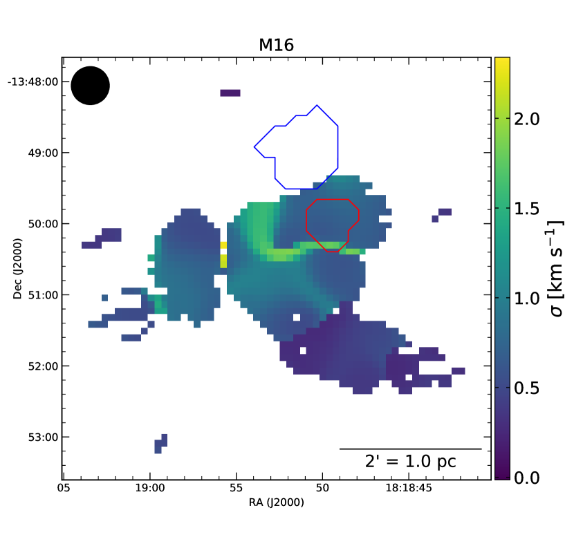
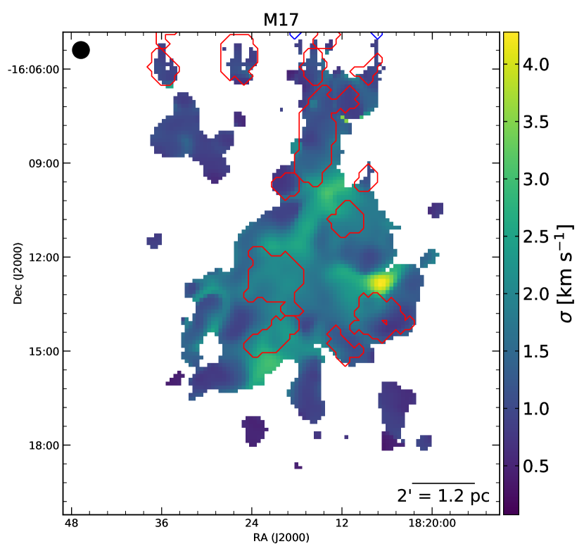
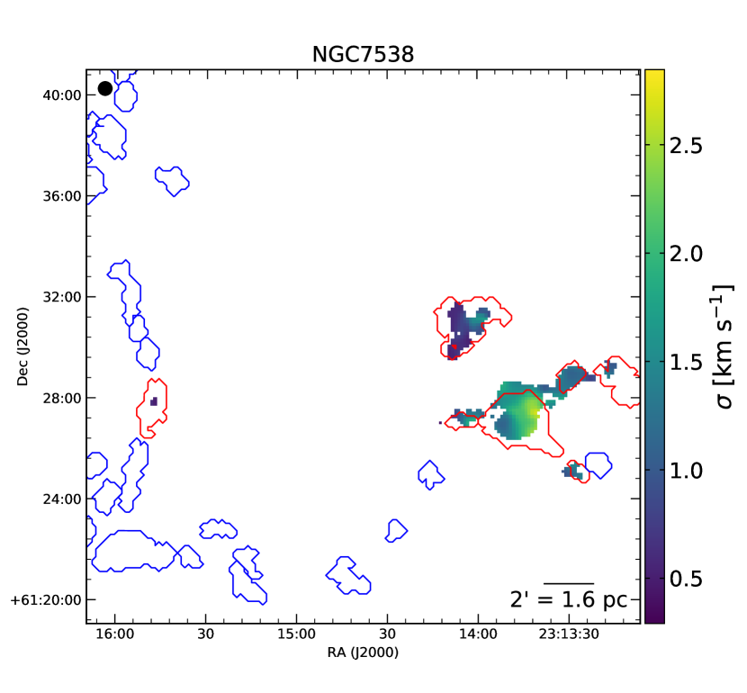
Figure 50: Same as Figure 49 for M16 (top left), M17 (top right), and NGC7538 (bottom).

In addition to external pressure, the magnetic field may also play an important role in the virial stability of the ammonia-identified leaves. For instance, both observations (e.g., Tan et al., 2013; Pillai et al., 2015) and simulations (e.g. Peters et al., 2011) suggest that magnetic fields are equally as important as turbulence and gravity for high-mass star formation. Although we currently lack large-scale magnetic field measurements for the KEYSTONE clouds, Auddy et al. (2019) have recently developed a “core field structure” model that predicts the magnetic field strength and fluctuation profile using dense gas kinematics. We reserve a detailed analysis of the clump magnetic fields, however, to a future KEYSTONE paper.

5 Summary

We have presented initial observations and results from KFPA Examinations of Young STellar Object Natal Environments (KEYSTONE), a survey of filamentary dense gas structure in eleven GMCs (Cygnus X North, Cygnus X South, M16, M17, MonR1, MonR2, NGC2264, NGC7538, Rosette, W3, and W48) at distances of $0.9-3.0$ kpc. We identified 856 dense gas clumps, traced by NH₃ (1,1) emission, across all the observed clouds using a dendrogram analysis. Simultaneous line fitting of the NH₃ (1,1) and (2,2) emission provided estimates of kinetic gas temperature, centroid velocity, velocity dispersion, and para-NH₃ column density for the dense gas. These parameter maps and the NH₃ (1,1) and (2,2) data cubes are publicly available.

The ammonia parameter maps were used to derive virial stability parameters for each dense gas structure identified, providing insight into whether or not the gravitational potential energy of the structures is enough to overcome their internal kinetic energies in the absence of magnetic fields or external pressure. HOBYS Herschel Space Observatory observations of dust continuum emission were utilized to create H₂ column density maps, identify young protostellar candidates, and identify filamentary structures in each region. James Clerk Maxwell Telescope observations of C¹⁸O $(3-2)$ emission were accessed to determine the turbulent pressure applied by the ambient molecular cloud upon a subset of the dendrogram-identified dense gas structures. Our main results are listed below:

1. Significant variations in kinetic gas temperature are observed between clouds, with median $T_{K}=11.4\pm 2.2$ K in the coldest region (MonR1) and $T_{K}=23.0\pm 6.5$ K in the warmest (M17). The velocity dispersion distributions are more similar between clouds, with characteristic median values of $0.3-0.7$ km s^-1.

2. Of the 835 ammonia-identified clumps with mass estimates, 523 ($\sim 63~{}\%$) have virial parameters less than two, suggesting the mass of those structures is gravitationally bound and more susceptible to gravitational collapse when neglecting the effects of magnetic fields or external pressure. Similar analyses in nearby, low-mass star-forming clouds have found much higher rates of gravitationally bound ammonia-identified cores, which may suggest ammonia is more widespread in GMCs than in nearby clouds or that gravity is more important to structure stability at small scales.

3. The fraction of ammonia-identified clumps that are spatially coincident with filaments identified in the H₂ column density maps ranges from 0.35 in Cygnus X South to 1.0 in W3-west. These values are consistent with core on-filament fractions found from dust continuum observations of nearby star-forming regions, which tend to be from $\sim 0.4-0.8$ depending on the cloud and core class considered.

4. On- and off-filament clumps show no substantial differences in their virial parameter, mass, radius, temperature, and velocity dispersion distributions. We do find, however, a tendency for clouds with low dense gas mass to have a higher fraction of on-filament clumps. These findings may indicate that filaments play a lesser role in the star formation process of high-mass GMCs. In those environments, dense gas may be more widespread allowing for clump formation to be equally as likely on and off filaments. In lower mass environments where dense gas is less widespread, however, clump formation may be limited to the filaments that harbor the main supply of dense gas.

5. In several regions there are “hubs” or “ridges” of dense gas that have much higher masses and lower virial parameters than the other clumps in their respective cloud. These hubs and ridges tend to be located at the intersections of multiple filaments or located near/within a single filament, are often associated with H₂O maser emission, and typically host multiple protostars. Based on these characteristics, hubs may be the sites of future cluster formation.

6. When considering the external pressure exerted on the clumps, most are considered sub-virial and pressure-dominated structures. This characteristic state may indicate that high-mass clumps spend the majority of their lifetime confined by external pressure. Over time, as the clumps accrete mass from their surroundings, they may gain enough mass to be gravitationally dominated and undergo gravitational collapse or fragmentation.

6 Future Work

Although it was not the focus of this paper, a key use-case of the KEYSTONE data is the analysis of filament kinematics in GMCs. For instance, in regards to the observed spatial relationship between massive young stellar objects and stellar clusters with filament intersections, the KEYSTONE data could be used to determine: 1) whether or not the observed clumps and filaments are truly velocity coherent structures (Pineda et al., 2010; Chen et al., 2019a), and 2) if the mass flow rates along them are large enough to produce MYSOs. Several independent studies have already measured gas motions in individual filaments such as Serpens South (Kirk et al., 2013a; Friesen et al., 2013), G035.39-00.33 (Henshaw et al., 2013), DR21 (Schneider et al., 2010a), W43-MM1 (Nguyen-Lu’o’ng et al., 2013), M17SW (Chen et al., 2019b), and eight other high-mass filaments (Lu et al., 2018), noting that the observed mass flow rates could supply the mass required to assemble the stellar clusters at their centres. Similarly, observations of the Large Magellanic Cloud by Fukui et al. (2015) showed two separate instances of MYSOs forming at the centers of adjoining filaments that have gas flowing into the central junction. Svoboda et al. (2016) and Motte et al. (2018a) also contend that such mass flow onto sites of cluster formation is prominent throughout Galactic high-mass star-forming regions, providing the mass build-up and compression necessary to form stellar clusters. These studies, however, have focused primarily on regions that have already formed clusters/MYSOs and do not address the conditions of the parental clumps, i.e., the dense gas out of which stellar clusters form, prior to the onset of star formation. As such, the gas velocity patterns of those regions are susceptible to distortions due to stellar feedback, which raises questions about the applicability of their kinematic measurements. Furthermore, observations after the onset of star formation cannot be used to decipher whether clumps form before or after filaments collide to form intersections. Using the clump catalog presented in this paper, in conjunction with an analysis of the adjacent filament kinematics, it is now possible to investigate these questions across multiple high-mass star-forming environments.

In addition to dense gas kinematics, the KEYSTONE data can provide insight into temperature and chemistry variations as a function of environment within GMCs. For example, the KEYSTONE observations of the NH₃ (1,1), (2,2), (3,3), (4,4), and (5,5) transitions probe a range of gas temperatures up to $\sim$ 200 K. Since dust temperatures derived from Herschel data become increasingly uncertain above 20 K as the spectral energy distribution peak moves toward wavelengths shorter than 160 $\mu$m (Chen et al., 2016), ammonia-derived gas temperatures will be important for understanding how the OB associations are impacting the star formation in the KEYSTONE target clouds. Furthermore, the KEYSTONE observations will constrain the abundances of NH₃ in GMCs. These abundances, in combination with the gas temperatures, will provide a way to understand how temperature impacts the formation/destruction of ammonia in GMCs.

Appendix

Appendix A Distance Dependence of Virial Parameters

The virial analysis presented in this paper used the native KEYSTONE resolution for all clouds analyzed, despite the cloud distances ranging from 0.9 kpc to 3 kpc. Such distance variations provide a factor of $\sim 3$ range of linear spatial resolutions, which may lead to different types of structures (in terms of size and mass) being identified in each cloud. To test whether or not the distance dependence has any influence on the main results of this paper, we convolved the NH₃ (1,1) and (2,2) cubes for NGC 2264, MonR1, and MonR2 ($d=0.9$ kpc, $\theta\sim 0.13$ pc), the closest clouds in KEYSTONE, to the linear resolution of W48 ($d=3.0$ kpc, $\theta\sim 0.45$ pc), the most distant cloud observed. This process degrades the resolution of the observations by a factor of $3.0/0.9\sim 3.3$ to a final resolution of $\sim 103\arcsec$. Following a similar distance bias analysis by Baldeschi et al. (2017) on Herschel maps, we also downsampled the cubes by the same factor along each spatial axis. Finally, Gaussian noise with a mean of zero and standard deviation of $s_{N}\sqrt{1-d_{0}/d_{1}}$ is added to the cubes, where $s_{N}$ is the median of the original cube’s RMS map, $d_{0}$ is 0.9 pc and $d_{1}$ is 3.0 kpc. This noise addition attempts to return the native RMS level to the convolved and resampled cubes, which have lower noise levels due to the spatial averaging.

These processes allow us to simulate what might be observed if NGC 2264, MonR1, and MonR2 were at a distance of 3 kpc. The convolved, downsampled, noise-injected cubes were then run through the line-fitting pipeline to produce a new set of ammonia parameter maps and integrated intensity maps. Finally, we repeat the virial analysis presented in Section 3.5 using the new set of maps and assuming their distance is 3.0 kpc.

In Figures 51-53, we compare the results of the original virial analyses in NGC 2264, MonR1, and MonR2 to their distance-adjusted virial analysis. Leaves from the original analysis that fall within a leaf identified in the distance-adjusted analysis are tagged with a specific color in each plot of Figures 51-53. As expected, much fewer structures are identified by the dendrogram in the distance-adjusted analysis. Many of the small structures in the original analysis are lumped together into a single large structure in the distance-adjusted analysis due to the lower resolution. In terms of virial parameters, the structures in the distance-adjusted analysis are all gravitationally bound. This distance bias is likely why more bound structures are observed in W48 than these closer clouds. At 900 pc, NGC2264, MonR1, and MonR2 represent the extreme examples of the distance bias in our sample. The impact will undoubtedly be less for the moderate distance clouds in our sample (e.g., Cygnus X, W3, NGC7538, etc.), for which the distance difference is lower. This statement is echoed by the fact that many of the cloud attributes analyzed in this paper (e.g., dense gas mass, leaf on-filament fraction, number of leaves, etc.) do not depend strongly on cloud distance (see Section 3.7 and Figure 44). Nevertheless, we are indeed tracing different scales in the star formation hierarchy by including a range of cloud distances in our analysis. Future high-resolution observations of the more distant KEYSTONE targets with the Karl G. Jansky Very Large Array (VLA) or Next Generation VLA (ngVLA) could provide the means to compare cloud structures between clouds on more similar spatial scales.

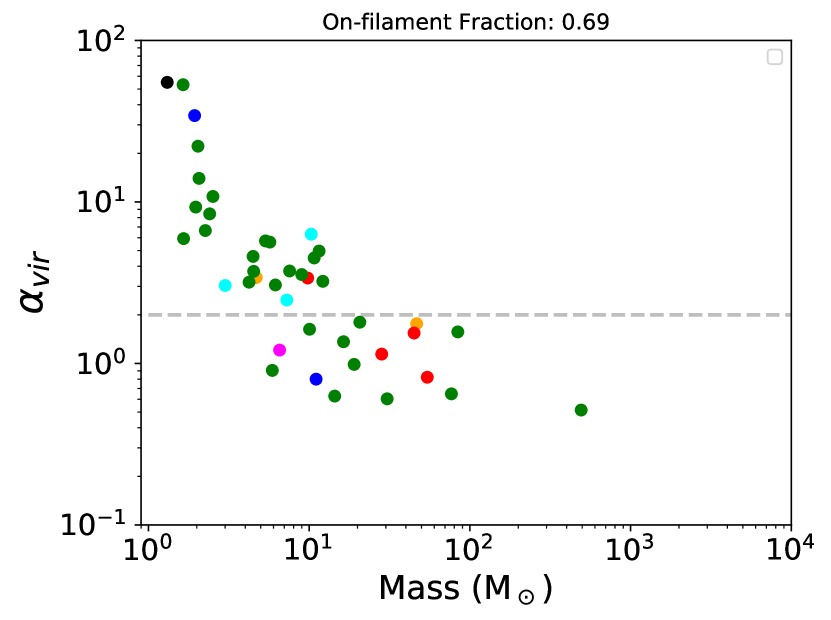
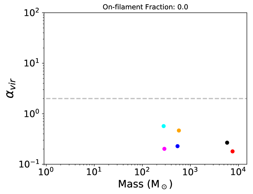
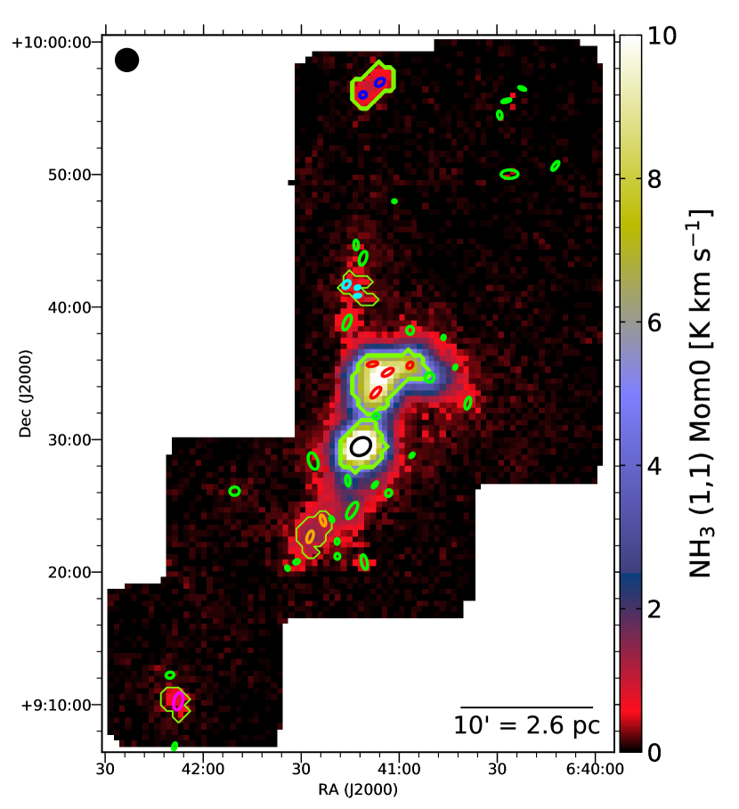
Figure 51: Top row: Leaf virial parameters in NGC2264 using native KEYSTONE resolution (left) and after convolving the NH₃ (1,1) and (2,2) cubes to the linear resolution of W48 ($\theta\sim 0.45$ pc), downsampling the number of pixels, adding white noise, and re-running the full analysis. Bottom: Integrated intensity map obtained using the convolved NH₃ (1,1) cube. Ellipses represent the peaks of leaves identified when using the native resolution data. The green dendrogram masks show the extent of the leaves identified using the convolved data. Ellipses falling within a dendrogram mask were tagged as a colored pair in the top row plots.

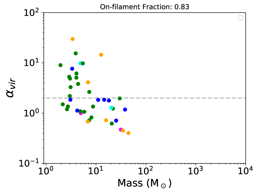
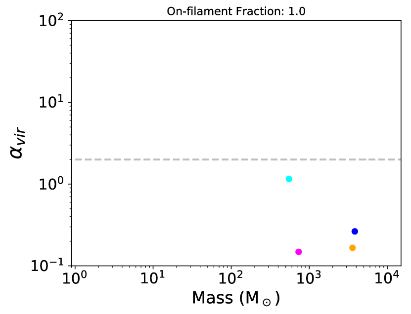
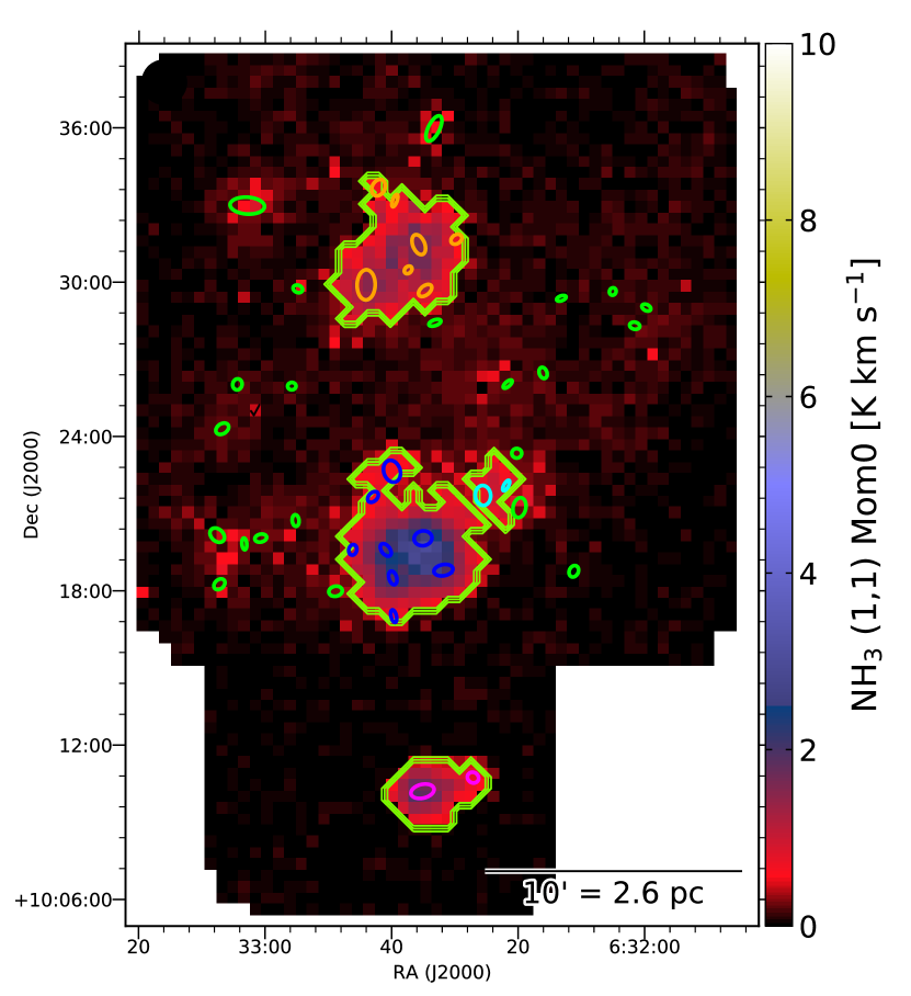
Figure 52: Same as Figure 51 for MonR1.

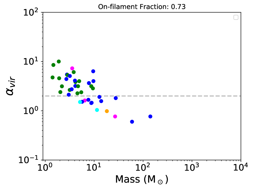
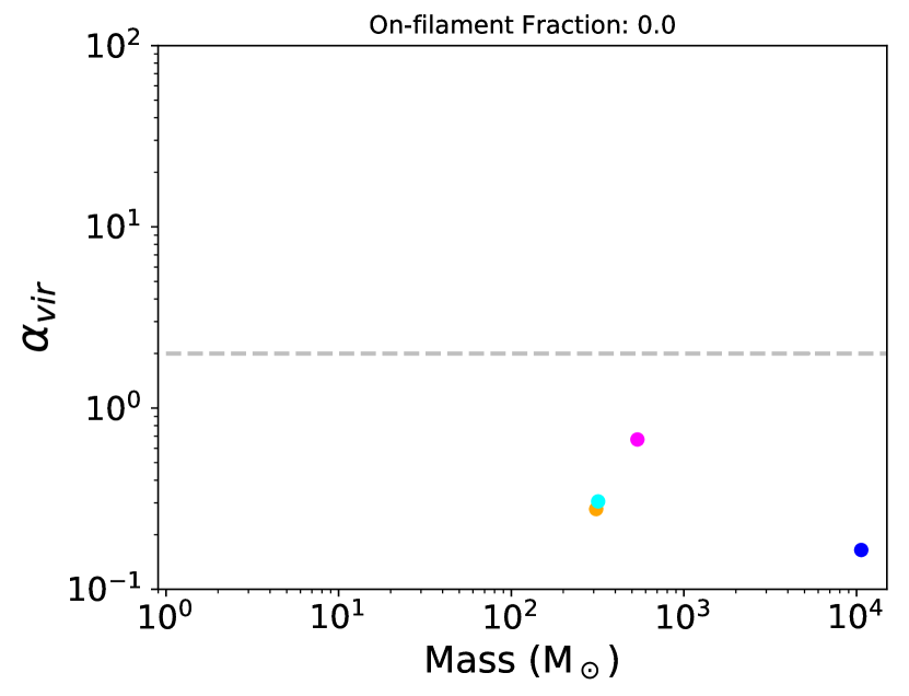
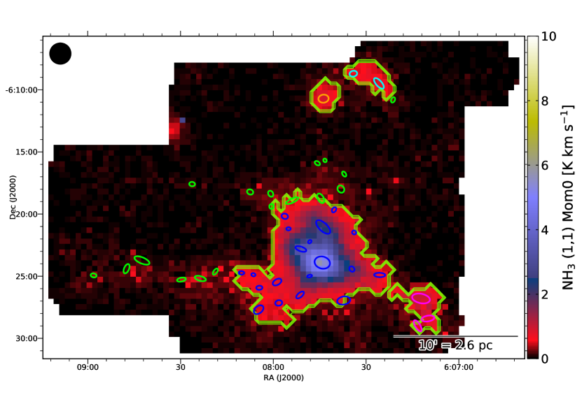
Figure 53: Same as Figure 51 for MonR2.

References

- Adams et al. (1979) Adams, M. T., Strom, K. M., & Strom, S. E. 1979, ApJ, 230, L183
- André et al. (2010) André, P., Men’shchikov, A., Bontemps, S., et al. 2010, A&A, 518, L102
- Astropy Collaboration et al. (2013) Astropy Collaboration, Robitaille, T. P., Tollerud, E. J., et al. 2013, A&A, 558, A33
- Auddy et al. (2019) Auddy, S., Myers, P. C., Basu, S., et al. 2019, ApJ, 872, 207
- Baldeschi et al. (2017) Baldeschi, A., Elia, D., Molinari, S., et al. 2017, MNRAS, 466, 3682
- Ballesteros-Paredes et al. (2018) Ballesteros-Paredes, J., Vázquez-Semadeni, E., Palau, A., & Klessen, R. S. 2018, MNRAS, 479, 2112
- Baxter et al. (2009) Baxter, E. J., Covey, K. R., Muench, A. A., et al. 2009, AJ, 138, 963
- Bertoldi & McKee (1992) Bertoldi, F., & McKee, C. F. 1992, ApJ, 395, 140
- Billington et al. (2019) Billington, S. J., Urquhart, J. S., Figura, C., Eden, D. J., & Moore, T. J. T. 2019, MNRAS, 483, 3146
- Blitz & Stark (1986) Blitz, L., & Stark, A. A. 1986, ApJ, 300, L89
- Blitz & Thaddeus (1980) Blitz, L., & Thaddeus, P. 1980, ApJ, 241, 676
- Bohlin et al. (1978) Bohlin, R. C., Savage, B. D., & Drake, J. F. 1978, ApJ, 224, 132
- Bonatto et al. (2006) Bonatto, C., Santos, Jr., J. F. C., & Bica, E. 2006, A&A, 445, 567
- Bonnell et al. (2003) Bonnell, I. A., Bate, M. R., & Vine, S. G. 2003, MNRAS, 343, 413
- Bontemps et al. (2010) Bontemps, S., Motte, F., Csengeri, T., & Schneider, N. 2010, A&A, 524, A18
- Boyden et al. (2016) Boyden, R. D., Koch, E. W., Rosolowsky, E. W., & Offner, S. S. R. 2016, ApJ, 833, 233
- Boyden et al. (2018) Boyden, R. D., Offner, S. S. R., Koch, E. W., & Rosolowsky, E. W. 2018, ApJ, 860, 157
- Bresnahan et al. (2018) Bresnahan, D., Ward-Thompson, D., Kirk, J. M., et al. 2018, A&A, 615, A125
- Burkhart (2018) Burkhart, B. 2018, ApJ, 863, 118
- Campbell (1984) Campbell, B. 1984, ApJ, 282, L27
- Carpenter et al. (1997) Carpenter, J. M., Meyer, M. R., Dougados, C., Strom, S. E., & Hillenbrand, L. A. 1997, AJ, 114, 198
- Castelaz et al. (1985) Castelaz, M. W., Grasdalen, G. L., Hackwell, J. A., Capps, R. W., & Thompson, D. 1985, AJ, 90, 1113
- Chen et al. (2019a) Chen, H. H.-H., Pineda, J. E., Goodman, A. A., et al. 2019a, ApJ, 877, 93
- Chen et al. (2019b) Chen, H.-R. V., Zhang, Q., Wright, M. C. H., et al. 2019b, ApJ, 875, 24
- Chen et al. (2016) Chen, M. C.-Y., Di Francesco, J., Johnstone, D., et al. 2016, ApJ, 826, 95
- Ching et al. (2017) Ching, T.-C., Lai, S.-P., Zhang, Q., et al. 2017, ApJ, 838, 121
- Colley (1980) Colley, D. 1980, MNRAS, 193, 495
- Comerón et al. (2019) Comerón, F., Djupvik, A. A., Torra, J., Schneider, N., & Pasquali, A. 2019, A&A, 622, A134
- Comerón & Pasquali (2012) Comerón, F., & Pasquali, A. 2012, A&A, 543, A101
- Contreras et al. (2017) Contreras, Y., Rathborne, J. M., Guzman, A., et al. 2017, MNRAS, 466, 340
- Csengeri et al. (2011a) Csengeri, T., Bontemps, S., Schneider, N., Motte, F., & Dib, S. 2011a, A&A, 527, A135
- Csengeri et al. (2011b) Csengeri, T., Bontemps, S., Schneider, N., et al. 2011b, ApJ, 740, L5
- Cunningham et al. (2018) Cunningham, A. J., Krumholz, M. R., McKee, C. F., & Klein, R. I. 2018, MNRAS, 476, 771
- Dahm (2008) Dahm, S. E. 2008, The Young Cluster and Star Forming Region NGC 2264 (ASP), 966
- Di Francesco et al. (2007) Di Francesco, J., Evans, II, N. J., Caselli, P., et al. 2007, Protostars and Planets V, 17
- Di Francesco et al. (2019, in prep) Di Francesco, J., Keown, J., Ladjelate, B., et al. 2019, in prep, ApJ
- Di Francesco et al. (2010) Di Francesco, J., Sadavoy, S., Motte, F., et al. 2010, A&A, 518, L91
- Didelon et al. (2015) Didelon, P., Motte, F., Tremblin, P., et al. 2015, A&A, 584, A4
- Dobashi et al. (2014) Dobashi, K., Matsumoto, T., Shimoikura, T., et al. 2014, ApJ, 797, 58
- Duarte-Cabral et al. (2014) Duarte-Cabral, A., Bontemps, S., Motte, F., et al. 2014, A&A, 570, A1
- Duarte-Cabral et al. (2013) —. 2013, A&A, 558, A125
- Dunham et al. (2011) Dunham, M. K., Rosolowsky, E., Evans, II, N. J., Cyganowski, C., & Urquhart, J. S. 2011, ApJ, 741, 110
- Dunham et al. (2010) Dunham, M. K., Rosolowsky, E., Evans, II, N. J., et al. 2010, ApJ, 717, 1157
- Elia & Pezzuto (2016) Elia, D., & Pezzuto, S. 2016, MNRAS, 461, 1328
- Elmegreen et al. (1979) Elmegreen, B. G., Lada, C. J., & Dickinson, D. F. 1979, ApJ, 230, 415
- Evans et al. (2005) Evans, C. J., Smartt, S. J., Lee, J.-K., et al. 2005, A&A, 437, 467
- Falgarone & Puget (1986) Falgarone, E., & Puget, J. L. 1986, A&A, 162, 235
- Fallscheer et al. (2013) Fallscheer, C., Reid, M. A., Di Francesco, J., et al. 2013, ApJ, 773, 102
- Federrath (2016) Federrath, C. 2016, MNRAS, 457, 375
- Field et al. (2011) Field, G. B., Blackman, E. G., & Keto, E. R. 2011, MNRAS, 416, 710
- Friesen et al. (2016) Friesen, R. K., Bourke, T. L., Di Francesco, J., Gutermuth, R., & Myers, P. C. 2016, ApJ, 833, 204
- Friesen et al. (2013) Friesen, R. K., Medeiros, L., Schnee, S., et al. 2013, MNRAS, 436, 1513
- Friesen et al. (2017) Friesen, R. K., Pineda, J. E., co-PIs, et al. 2017, ApJ, 843, 63
- Fukui et al. (2015) Fukui, Y., et al. 2015, ApJ, 807, L4
- Gao & Solomon (2004) Gao, Y., & Solomon, P. M. 2004, ApJ, 606, 271
- Gatley et al. (1979) Gatley, I., Becklin, E. E., Sellgren, K., & Werner, M. W. 1979, ApJ, 233, 575
- Ginsburg & Mirocha (2011) Ginsburg, A., & Mirocha, J. 2011, PySpecKit: Python Spectroscopic Toolkit, Astrophysics Source Code Library, ascl:1109.001
- Ginsburg et al. (2013) Ginsburg, A., Glenn, J., Rosolowsky, E., et al. 2013, ApJS, 208, 14
- Goodman et al. (2009) Goodman, A. A., Rosolowsky, E. W., Borkin, M. A., et al. 2009, Nature, 457, 63
- Gritschneder et al. (2010) Gritschneder, M., Burkert, A., Naab, T., & Walch, S. 2010, ApJ, 723, 971
- Guesten & Fiebig (1988) Guesten, R., & Fiebig, D. 1988, A&A, 204, 253
- Guilloteau et al. (1983) Guilloteau, S., Wilson, T. L., Martin, R. N., Batria, W., & Pauls, T. A. 1983, A&A, 124, 322
- Hachisuka et al. (2006) Hachisuka, K., Brunthaler, A., Menten, K. M., et al. 2006, ApJ, 645, 337
- Hansen et al. (2012) Hansen, C. E., Klein, R. I., McKee, C. F., & Fisher, R. T. 2012, ApJ, 747, 22
- Hanson (2003) Hanson, M. M. 2003, ApJ, 597, 957
- Hennebelle (2013) Hennebelle, P. 2013, A&A, 556, A153
- Hennemann et al. (2012) Hennemann, M., et al. 2012, A&A, 543, L3
- Henshaw et al. (2013) Henshaw, J. D., et al. 2013, MNRAS, 428, 3425
- Hester et al. (1996) Hester, J. J., Scowen, P. A., Sankrit, R., et al. 1996, AJ, 111, 2349
- Heyer et al. (2006) Heyer, M. H., Williams, J. P., & Brunt, C. M. 2006, ApJ, 643, 956
- Hildebrand (1983) Hildebrand, R. H. 1983, QJRAS, 24, 267
- Hill et al. (2012a) Hill, T., André, P., Arzoumanian, D., et al. 2012a, A&A, 548, L6
- Hill et al. (2012b) Hill, T., Motte, F., Didelon, P., et al. 2012b, A&A, 542, A114
- Ho et al. (1979) Ho, P. T. P., Barrett, A. H., Myers, P. C., et al. 1979, ApJ, 234, 912
- Ho & Townes (1983) Ho, P. T. P., & Townes, C. H. 1983, ARA&A, 21, 239
- Hoffman (2012) Hoffman, I. M. 2012, ApJ, 759, 76
- Hoffman & Seojin Kim (2011) Hoffman, I. M., & Seojin Kim, S. 2011, ApJ, 739, L15
- Hoffmeister et al. (2008) Hoffmeister, V. H., Chini, R., Scheyda, C. M., et al. 2008, ApJ, 686, 310
- Hogge et al. (2018) Hogge, T., Jackson, J., Stephens, I., et al. 2018, ApJS, 237, 27
- Johnston et al. (1989) Johnston, K. J., Stolovy, S. R., Wilson, T. L., Henkel, C., & Mauersberger, R. 1989, ApJ, 343, L41
- Kallas & Reich (1980) Kallas, E., & Reich, W. 1980, A&AS, 42, 227
- Kauffmann et al. (2008) Kauffmann, J., Bertoldi, F., Bourke, T. L., Evans, II, N. J., & Lee, C. W. 2008, A&A, 487, 993
- Kauffmann & Pillai (2010) Kauffmann, J., & Pillai, T. 2010, ApJ, 723, L7
- Kauffmann et al. (2013) Kauffmann, J., Pillai, T., & Goldsmith, P. F. 2013, ApJ, 779, 185
- Keown et al. (2017) Keown, J., Di Francesco, J., Kirk, H., et al. 2017, ApJ, 850, 3
- Kerr et al. (2019) Kerr, R., Kirk, H., Di Francesco, J., et al. 2019, ApJ, 874, 147
- Kirk et al. (2006) Kirk, H., Johnstone, D., & Di Francesco, J. 2006, ApJ, 646, 1009
- Kirk et al. (2013a) Kirk, H., Myers, P. C., Bourke, T. L., et al. 2013a, ApJ, 766, 115
- Kirk et al. (2017) Kirk, H., Friesen, R. K., Pineda, J. E., et al. 2017, ApJ, 846, 144
- Kirk et al. (2013b) Kirk, J. M., Ward-Thompson, D., Palmeirim, P., et al. 2013b, MNRAS, 432, 1424
- Knödlseder (2000) Knödlseder, J. 2000, A&A, 360, 539
- Koch et al. (2017) Koch, E. W., Ward, C. G., Offner, S., Loeppky, J. L., & Rosolowsky, E. W. 2017, MNRAS, 471, 1506
- Könyves et al. (2010) Könyves, V., André, P., Men’shchikov, A., et al. 2010, A&A, 518, L106
- Könyves et al. (2015) —. 2015, A&A, 584, A91
- Krumholz & McKee (2008) Krumholz, M. R., & McKee, C. F. 2008, Nature, 451, 1082
- Kryukova et al. (2014) Kryukova, E., Megeath, S. T., Hora, J. L., et al. 2014, AJ, 148, 11
- Kun et al. (2008) Kun, M., Kiss, Z. T., & Balog, Z. 2008, Star Forming Regions in Cepheus (ASP), 136
- Kurono et al. (2013) Kurono, Y., Saito, M., Kamazaki, T., Morita, K.-I., & Kawabe, R. 2013, ApJ, 765, 85
- Kutner et al. (1979) Kutner, M. L., Dickman, R. L., Tucker, K. D., & Machnik, D. E. 1979, ApJ, 232, 724
- Lada (1976) Lada, C. J. 1976, ApJS, 32, 603
- Lada et al. (2012) Lada, C. J., Forbrich, J., Lombardi, M., & Alves, J. F. 2012, ApJ, 745, 190
- Lada (1992) Lada, E. A. 1992, ApJ, 393, L25
- Lang & Willson (1980) Lang, K. R., & Willson, R. F. 1980, ApJ, 238, 867
- Larson (1981) Larson, R. B. 1981, MNRAS, 194, 809
- Lee et al. (2014) Lee, K. I., Fernández-López, M., Storm, S., et al. 2014, ApJ, 797, 76
- Li et al. (2013) Li, D., Kauffmann, J., Zhang, Q., & Chen, W. 2013, ApJ, 768, L5
- Li et al. (2016) Li, G.-X., Urquhart, J. S., Leurini, S., et al. 2016, A&A, 591, A5
- Liu et al. (2018) Liu, T., Li, P. S., Juvela, M., et al. 2018, ApJ, 859, 151
- Lombardi et al. (2011) Lombardi, M., Alves, J., & Lada, C. J. 2011, A&A, 535, A16
- Lovas (2004) Lovas, F. J. 2004, Journal of Physical and Chemical Reference Data, 33, 177
- Lu et al. (2018) Lu, X., Zhang, Q., Liu, H. B., et al. 2018, ApJ, 855, 9
- Mairs et al. (2014) Mairs, S., Johnstone, D., Offner, S. S. R., & Schnee, S. 2014, ApJ, 783, 60
- Mallick et al. (2014) Mallick, K. K., Ojha, D. K., Tamura, M., et al. 2014, MNRAS, 443, 3218
- Mangum et al. (2007) Mangum, J. G., Emerson, D. T., & Greisen, E. W. 2007, A&A, 474, 679
- Mangum et al. (1991) Mangum, J. G., Wootten, A., & Mundy, L. G. 1991, ApJ, 378, 576
- Margulis & Lada (1986) Margulis, M., & Lada, C. J. 1986, ApJ, 309, L87
- Marsh et al. (2016) Marsh, K. A., Kirk, J. M., André, P., et al. 2016, MNRAS, 459, 342
- McKee (1989) McKee, C. F. 1989, ApJ, 345, 782
- Megeath et al. (1996) Megeath, S. T., Herter, T., Beichman, C., et al. 1996, A&A, 307, 775
- Megeath et al. (2008) Megeath, S. T., Townsley, L. K., Oey, M. S., & Tieftrunk, A. R. 2008, Low and High Mass Star Formation in the W3, W4, and W5 Regions (ASP), 264
- Men’shchikov (2013) Men’shchikov, A. 2013, A&A, 560, A63
- Men’shchikov et al. (2012) Men’shchikov, A., André, P., Didelon, P., et al. 2012, A&A, 542, A81
- Men’shchikov et al. (2010) —. 2010, A&A, 518, L103
- Merello et al. (2019) Merello, M., Molinari, S., Rygl, K. L. J., et al. 2019, MNRAS, 483, 5355
- Minier et al. (2000) Minier, V., Booth, R. S., & Conway, J. E. 2000, A&A, 362, 1093
- Minier et al. (2013) Minier, V., Tremblin, P., Hill, T., et al. 2013, A&A, 550, A50
- Miville-Deschênes et al. (2010) Miville-Deschênes, M.-A., Martin, P. G., Abergel, A., et al. 2010, A&A, 518, L104
- Molinari et al. (2011) Molinari, S., Schisano, E., Faustini, F., et al. 2011, A&A, 530, A133
- Molinari et al. (2010) Molinari, S., Swinyard, B., Bally, J., et al. 2010, PASP, 122, 314
- Montalban et al. (1990) Montalban, J., Bachiller, R., Martin-Pintado, J., Tafalla, M., & Gomez-Gonzalez, J. 1990, A&A, 233, 527
- Moscadelli et al. (2009) Moscadelli, L., Reid, M. J., Menten, K. M., et al. 2009, ApJ, 693, 406
- Motte et al. (2018a) Motte, F., Bontemps, S., & Louvet, F. 2018a, ARA&A, 56, 41
- Motte et al. (2007) Motte, F., Bontemps, S., Schilke, P., et al. 2007, A&A, 476, 1243
- Motte et al. (2010) Motte, F., Zavagno, A., Bontemps, S., et al. 2010, A&A, 518, L77
- Motte et al. (2018b) Motte, F., Nony, T., Louvet, F., et al. 2018b, Nature Astronomy, 2, 478
- Myers (2009) Myers, P. C. 2009, ApJ, 700, 1609
- Nakano et al. (2017) Nakano, M., Soejima, T., Chibueze, J. O., et al. 2017, PASJ, 69, 16
- Naranjo-Romero et al. (2015) Naranjo-Romero, R., Vázquez-Semadeni, E., & Loughnane, R. M. 2015, ApJ, 814, 48
- Nguyen Luong et al. (2011) Nguyen Luong, Q., Motte, F., Hennemann, M., et al. 2011, A&A, 535, A76
- Nguyen-Lu’o’ng et al. (2013) Nguyen-Lu’o’ng, Q., Motte, F., Carlhoff, P., et al. 2013, ApJ, 775, 88
- Nishimura et al. (2017) Nishimura, A., Costes, J., Inaba, T., et al. 2017, arXiv e-prints - Submitted to PASJ, arXiv:1706.06002
- Nishimura et al. (2018) Nishimura, A., Minamidani, T., Umemoto, T., et al. 2018, PASJ, 70, S42
- Oey et al. (2005) Oey, M. S., Watson, A. M., Kern, K., & Walth, G. L. 2005, AJ, 129, 393
- Offner et al. (2013) Offner, S. S. R., Bisbas, T. G., Viti, S., & Bell, T. A. 2013, ApJ, 770, 49
- Offner & Chaban (2017) Offner, S. S. R., & Chaban, J. 2017, ApJ, 847, 104
- Offner & Liu (2018) Offner, S. S. R., & Liu, Y. 2018, Nature Astronomy, 2, 896
- Ogura (1984) Ogura, K. 1984, PASJ, 36, 139
- Ohashi et al. (2016) Ohashi, S., Sanhueza, P., Chen, H.-R. V., et al. 2016, ApJ, 833, 209
- Ojha et al. (2004) Ojha, D. K., Tamura, M., Nakajima, Y., et al. 2004, ApJ, 608, 797
- Oliveira (2008) Oliveira, J. M. 2008, Star Formation in the Eagle Nebula (ASP), 599
- Oliver et al. (1996) Oliver, R. J., Masheder, M. R. W., & Thaddeus, P. 1996, A&A, 315, 578
- Olmi et al. (2010) Olmi, L., Araya, E. D., Chapin, E. L., et al. 2010, ApJ, 715, 1132
- Pagani & Nguyen-Q-Rieu (1987) Pagani, L. P., & Nguyen-Q-Rieu. 1987, A&A, 181, 112
- Palmeirim et al. (2013) Palmeirim, P., André, P., Kirk, J., et al. 2013, A&A, 550, A38
- Pattle et al. (2015) Pattle, K., Ward-Thompson, D., Kirk, J. M., et al. 2015, MNRAS, 450, 1094
- Pattle et al. (2017) —. 2017, MNRAS, 464, 4255
- Peretto et al. (2006) Peretto, N., André, P., & Belloche, A. 2006, A&A, 445, 979
- Pérez-Beaupuits et al. (2015) Pérez-Beaupuits, J. P., Stutzki, J., Ossenkopf, V., et al. 2015, A&A, 575, A9
- Peters et al. (2011) Peters, T., Banerjee, R., Klessen, R. S., & Mac Low, M.-M. 2011, ApJ, 729, 72
- Pillai et al. (2012) Pillai, T., Caselli, P., Kauffmann, J., et al. 2012, ApJ, 751, 135
- Pillai et al. (2015) Pillai, T., Kauffmann, J., Tan, J. C., et al. 2015, ApJ, 799, 74
- Pillai et al. (2011) Pillai, T., Kauffmann, J., Wyrowski, F., et al. 2011, A&A, 530, A118
- Pineda et al. (2010) Pineda, J. E., Goodman, A. A., Arce, H. G., et al. 2010, ApJ, 712, L116
- Pirogov (2009) Pirogov, L. E. 2009, Astronomy Reports, 53, 1127
- Planck Collaboration et al. (2014) Planck Collaboration, Abergel, A., Ade, P. A. R., et al. 2014, A&A, 571, A11
- Pokhrel et al. (2016) Pokhrel, R., Gutermuth, R., Ali, B., et al. 2016, MNRAS, 461, 22
- Polychroni et al. (2013) Polychroni, D., Schisano, E., Elia, D., et al. 2013, ApJ, 777, L33
- Povich et al. (2009) Povich, M. S., Churchwell, E., Bieging, J. H., et al. 2009, ApJ, 696, 1278
- Purcell et al. (2012) Purcell, C. R., Longmore, S. N., Walsh, A. J., et al. 2012, MNRAS, 426, 1972
- Qiu et al. (2011) Qiu, K., Zhang, Q., & Menten, K. M. 2011, ApJ, 728, 6
- Rapson et al. (2014) Rapson, V. A., Pipher, J. L., Gutermuth, R. A., et al. 2014, ApJ, 794, 124
- Rayner et al. (2017) Rayner, T. S. M., Griffin, M. J., Schneider, N., et al. 2017, A&A, 607, A22
- Redaelli et al. (2017) Redaelli, E., Alves, F. O., Caselli, P., et al. 2017, ApJ, 850, 202
- Reid & Wilson (2005) Reid, M. A., & Wilson, C. D. 2005, ApJ, 625, 891
- Rivera-Gálvez et al. (2015) Rivera-Gálvez, S., Román-Zúñiga, C. G., Jiménez-Bailón, E., et al. 2015, AJ, 150, 191
- Rivera-Ingraham et al. (2011) Rivera-Ingraham, A., Martin, P. G., Polychroni, D., & Moore, T. J. T. 2011, ApJ, 743, 39
- Rivera-Ingraham et al. (2013) Rivera-Ingraham, A., Martin, P. G., Polychroni, D., et al. 2013, ApJ, 766, 85
- Rivera-Ingraham et al. (2015) —. 2015, ApJ, 809, 81
- Rivera-Ingraham et al. (2016) Rivera-Ingraham, A., Ristorcelli, I., Juvela, M., et al. 2016, A&A, 591, A90
- Román-Zúñiga & Lada (2008) Román-Zúñiga, C. G., & Lada, E. A. 2008, Star Formation in the Rosette Complex (ASP), 928
- Rosolowsky & Leroy (2006) Rosolowsky, E., & Leroy, A. 2006, PASP, 118, 590
- Rosolowsky et al. (2010) Rosolowsky, E., Dunham, M. K., Ginsburg, A., et al. 2010, ApJS, 188, 123
- Rosolowsky et al. (2008) Rosolowsky, E. W., Pineda, J. E., Kauffmann, J., & Goodman, A. A. 2008, ApJ, 679, 1338
- Rygl et al. (2010) Rygl, K. L. J., Wyrowski, F., Schuller, F., & Menten, K. M. 2010, A&A, 515, A42
- Rygl et al. (2012) Rygl, K. L. J., Brunthaler, A., Sanna, A., et al. 2012, A&A, 539, A79
- Rygl et al. (2014) Rygl, K. L. J., Goedhart, S., Polychroni, D., et al. 2014, MNRAS, 440, 427
- Sandell et al. (2005) Sandell, G., Goss, W. M., & Wright, M. 2005, ApJ, 621, 839
- Sandell et al. (2003) Sandell, G., Wright, M., & Forster, J. R. 2003, ApJ, 590, L45
- Schilke et al. (1990) Schilke, P., Mauersberger, R., Walmsley, C. M., & Wilson, T. L. 1990, A&A, 227, 220
- Schlafly et al. (2014) Schlafly, E. F., Green, G., Finkbeiner, D. P., et al. 2014, ApJ, 786, 29
- Schneider et al. (2006) Schneider, N., Bontemps, S., Simon, R., et al. 2006, A&A, 458, 855
- Schneider et al. (2010a) Schneider, N., Csengeri, T., Bontemps, S., et al. 2010a, A&A, 520, A49
- Schneider et al. (1998) Schneider, N., Stutzki, J., Winnewisser, G., & Block, D. 1998, A&A, 335, 1049
- Schneider et al. (2010b) Schneider, N., Motte, F., Bontemps, S., et al. 2010b, A&A, 518, L83
- Schneider et al. (2011) Schneider, N., Bontemps, S., Simon, R., et al. 2011, A&A, 529, A1
- Schneider et al. (2012) Schneider, N., et al. 2012, A&A, 540, L11
- Schneider et al. (2015) Schneider, N., Bontemps, S., Girichidis, P., et al. 2015, MNRAS, 453, L41
- Schneider et al. (2016) Schneider, N., Bontemps, S., Motte, F., et al. 2016, A&A, 591, A40
- Schöier et al. (2005) Schöier, F. L., van der Tak, F. F. S., van Dishoeck, E. F., & Black, J. H. 2005, A&A, 432, 369
- Schuller et al. (2009) Schuller, F., Menten, K. M., Contreras, Y., et al. 2009, A&A, 504, 415
- Scoville et al. (1986) Scoville, N. Z., Sargent, A. I., Sanders, D. B., et al. 1986, ApJ, 303, 416
- Seifried & Walch (2015) Seifried, D., & Walch, S. 2015, MNRAS, 452, 2410
- Seo et al. (2015) Seo, Y. M., Shirley, Y. L., Goldsmith, P., et al. 2015, ApJ, 805, 185
- Shirley (2015) Shirley, Y. L. 2015, PASP, 127, 299
- Slysh et al. (1995) Slysh, V. I., Kalenskii, S. V., & Val’tts, I. E. 1995, ApJ, 442, 668
- Smith et al. (2014a) Smith, R. J., Glover, S. C. O., Clark, P. C., Klessen, R. S., & Springel, V. 2014a, MNRAS, 441, 1628
- Smith et al. (2014b) Smith, R. J., Glover, S. C. O., & Klessen, R. S. 2014b, MNRAS, 445, 2900
- Stephens et al. (2016) Stephens, I. W., Jackson, J. M., Whitaker, J. S., et al. 2016, ApJ, 824, 29
- Stutzki & Guesten (1990) Stutzki, J., & Guesten, R. 1990, ApJ, 356, 513
- Stutzki et al. (1988) Stutzki, J., Stacey, G. J., Genzel, R., et al. 1988, ApJ, 332, 379
- Sugiyama et al. (2008) Sugiyama, K., Fujisawa, K., Doi, A., et al. 2008, PASJ, 60, 23
- Surcis et al. (2012) Surcis, G., Vlemmings, W. H. T., van Langevelde, H. J., & Hutawarakorn Kramer, B. 2012, A&A, 541, A47
- Svoboda et al. (2016) Svoboda, B. E., et al. 2016, ApJ, 822, 59
- Tan et al. (2013) Tan, J. C., Kong, S., Butler, M. J., Caselli, P., & Fontani, F. 2013, ApJ, 779, 96
- Teixeira et al. (2012) Teixeira, P. S., Lada, C. J., Marengo, M., & Lada, E. A. 2012, A&A, 540, A83
- Thronson & Lada (1983) Thronson, Jr., H. A., & Lada, C. J. 1983, ApJ, 269, 175
- Tieftrunk et al. (1997) Tieftrunk, A. R., Gaume, R. A., Claussen, M. J., Wilson, T. L., & Johnston, K. J. 1997, A&A, 318, 931
- Tieftrunk et al. (1998) Tieftrunk, A. R., Megeath, S. T., Wilson, T. L., & Rayner, J. T. 1998, A&A, 336, 991
- Tigé et al. (2017) Tigé, J., Motte, F., Russeil, D., et al. 2017, A&A, 602, A77
- Traficante et al. (2018) Traficante, A., Duarte-Cabral, A., Elia, D., et al. 2018, MNRAS, 477, 2220
- Tremblin et al. (2013) Tremblin, P., Minier, V., Schneider, N., et al. 2013, A&A, 560, A19
- Tremblin et al. (2014) Tremblin, P., Schneider, N., Minier, V., et al. 2014, A&A, 564, A106
- Urquhart et al. (2011) Urquhart, J. S., Morgan, L. K., Figura, C. C., et al. 2011, MNRAS, 418, 1689
- Urquhart et al. (2015) Urquhart, J. S., Figura, C. C., Moore, T. J. T., et al. 2015, MNRAS, 452, 4029
- Uyanıker et al. (2001) Uyanıker, B., Fürst, E., Reich, W., Aschenbach, B., & Wielebinski, R. 2001, A&A, 371, 675
- Vázquez-Semadeni et al. (2017) Vázquez-Semadeni, E., González-Samaniego, A., & Colín, P. 2017, MNRAS, 467, 1313
- Vázquez-Semadeni et al. (2019) Vázquez-Semadeni, E., Palau, A., Ballesteros-Paredes, J., Gómez, G. C., & Zamora-Avilés, M. 2019, arXiv e-prints - Submitted to MNRAS, arXiv:1903.11247
- Vázquez-Semadeni et al. (2006) Vázquez-Semadeni, E., Ryu, D., Passot, T., González, R. F., & Gazol, A. 2006, ApJ, 643, 245
- Walsh et al. (1992) Walsh, J. R., Ogura, K., & Reipurth, B. 1992, MNRAS, 257, 110
- Wang et al. (2003) Wang, H., Yang, J., Wang, M., & Yan, J. 2003, AJ, 125, 842
- Wang et al. (2008) Wang, J., Townsley, L. K., Feigelson, E. D., et al. 2008, ApJ, 675, 464
- Ward-Thompson et al. (2010) Ward-Thompson, D., Kirk, J. M., André, P., et al. 2010, A&A, 518, L92
- Werner et al. (1979) Werner, M. W., Becklin, E. E., Gatley, I., et al. 1979, MNRAS, 188, 463
- White et al. (1999) White, G. J., Nelson, R. P., Holland, W. S., et al. 1999, A&A, 342, 233
- Wienen et al. (2012) Wienen, M., Wyrowski, F., Schuller, F., et al. 2012, A&A, 544, A146
- Williams et al. (2001) Williams, R. J. R., Ward-Thompson, D., & Whitworth, A. P. 2001, MNRAS, 327, 788
- Willson & Folch-Pi (1981) Willson, R. F., & Folch-Pi, F. J. 1981, AJ, 86, 1084
- Wilson et al. (2005) Wilson, B. A., Dame, T. M., Masheder, M. R. W., & Thaddeus, P. 2005, A&A, 430, 523
- Wilson & Mauersberger (1990) Wilson, T. L., & Mauersberger, R. 1990, A&A, 239, 305
- Wolf-Chase et al. (1995) Wolf-Chase, G. A., Walker, C. K., & Lada, C. J. 1995, ApJ, 442, 197
- Wright et al. (2014) Wright, N. J., Parker, R. J., Goodwin, S. P., & Drake, J. J. 2014, MNRAS, 438, 639
- Wu et al. (2005) Wu, J., Evans, II, N. J., Gao, Y., et al. 2005, ApJ, 635, L173
- Wu et al. (2010) Wu, J., Evans, II, N. J., Shirley, Y. L., & Knez, C. 2010, ApJS, 188, 313
- Xu et al. (2011) Xu, Y., Moscadelli, L., Reid, M. J., et al. 2011, ApJ, 733