Unit Level Modeling of Survey Data for Small Area Estimation Under Informative Sampling: A Comprehensive Overview with Extensions

Abstract

Model-based small area estimation is frequently used in conjunction with survey data in order to establish estimates for under-sampled or unsampled geographies. These models can be specified at either the area-level, or the unit-level, but unit-level models often offer potential advantages such as more precise estimates and easy spatial aggregation. Nevertheless, relative to area-level models, literature on unit-level models is less prevalent. In modeling small areas at the unit level, challenges often arise as a consequence of the informative sampling mechanism used to collect the survey data. This paper provides a comprehensive methodological review for unit-level models under informative sampling, with an emphasis on Bayesian approaches. To provide insight into the differences between methods, we conduct a simulation study that compares several of the described approaches. In addition, the methods used for simulation are further illustrated through an application to the American Community Survey. Finally, we present several extensions and areas for future research.

Keywords: Bayesian analysis, Informative sampling, Pseudo-likelihood, Small area estimation, Survey sampling.

1 Introduction

Government agencies have seen an increase in demand for data products in recent years. One trend that has accompanied this demand is the need for granular estimates of parameters of interest at small spatial scales or subdomains of the finite population. Typically, sample surveys are designed to provide reliable estimates of the parameters of interest for large domains. However, for some subpopulations, the area-specific sample size may be too small to produce estimates with adequate precision. The term small area is used to refer to any domain of interest, such as a geographic area or demographic cross classification, for which the domain-specific sample size is not large enough for reliable direct estimation. To improve precision, model-based methods can be used to ‘borrow strength,’ by relating the different areas of interest through use of linking models, and by introducing area-specific random effects and covariates. The Small Area Income and Poverty Estimates (SAIPE) program, and the Small Area Health Insurance Estimates (SAHIE) program within the U. S. Census Bureau are two examples of government programs which produce county and sub-county level estimates for different demographic cross classifications across the entire United States using small area estimation (SAE) methods (Luery,, 2011; Bauder et al.,, 2018). It can be difficult to generate small area estimates such as these for a number of reasons, including the fact that many geographic areas may have very limited sample sizes, if they have been sampled at all.

Models for SAE may be specified either at the area level or the unit level (see Rao and Molina,, 2015, for an overview of small area estimation methodology). Area-level models treat the direct estimate (for example, the survey-weighted estimate of a mean) as the response, and typically induce some type of smoothing across areas. In this way, the areas with limited sample sizes may “borrow strength” from areas with larger samples. While area-level models are popular, they are limited, in that it is difficult to make estimates and predictions at a geographic or demographic level that is finer than the level of the aggregated direct estimate.

In contrast, unit-level models use individual survey units as the response data, rather than the direct estimates. Use of unit-level models can overcome some of the limitations of area-level models, as they constitute a bottom-up approach (i.e., they utilize the finest scale of resolution of the data). Since model inputs are at the unit-level (person-level, household-level, or establishment-level), predictions and estimates can be made at the same unit-level, or aggregated up to any desired level. Unit-level modeling also has the added benefit of ensuring logical consistency of estimates at different geographic levels. For example, model-based county estimates are forced to aggregate to the corresponding state-level estimates, eliminating the need for ad hoc benchmarking. In addition, because the full unit-level data set is used in the modeling, rather than the summary statistics used with area-level models, there is potential for improved precision of estimated quantities.

Although unit-level models may lead to more precise estimates, that aggregate naturally across different spatial resolutions, they also introduce new challenges. Perhaps the biggest challenge is how to account for the survey design in the model. With area-level models, the survey design is incorporated into the model through specification of a sampling distribution (typically taken to be Gaussian) and inclusion of direct variance estimates. With unit-level models, accounting for the survey design is not as simple. One challenge is that the sample unit response may be dependent on the probability of selection, even after conditioning on the design variables. When the response variables are correlated with the sample selection variables, the sampling scheme is said to be informative, and in these scenarios, in order to avoid bias, it is critical to capture the sample design in the model by including the survey weights or the design variables used to construct the survey weights.

The aim of this paper is to present a comprehensive literature review of unit-level small area modeling strategies, with an emphasis on Bayesian approaches, and to evaluate a selection of these strategies by fitting different unit-level models on both simulated data, and on real American Community Survey (ACS) micro-data, thereby comparing model-based predictions and uncertainty estimates. In this paper we focus mainly on model specification and methods which incorporate informative sampling designs into the small area model. Some important, related issues, that will be outside the scope of this paper include issues related to measurement error and adjustments for nonresponse. Generally, we assume that observed survey weights have been modified to take into account nonresponse. We also avoid discussion on the relative merits of frequentist versus Bayesian methods for inference. In the simulation studies and data examples given in Sections 7 and 8, we fit three unit-level small area Bayesian models, with vague, proper priors on all unknown model parameters. Inference on the finite population parameters of interest is done using the posterior mean as a point estimate, and the posterior variance as a measure of uncertainty.

Some related work includes Hidiroglou and You, (2016), who present a simulation study to compare area-level and unit-level models, both fit in a frequentist setting. They fit their models under both informative and noninformative sampling, and found that overall the unit-level models lead to better interval coverage and more precise estimates. Gelman, (2007) discusses poststratification using survey data, and compares the implied weights of various models including hierarchical regression. Lumley et al., (2017) discuss general techniques for modeling survey data with included weights. They focus on frequentist pseudo-likelihood estimation as well as hypothesis testing. Chapter 7 of Rao and Molina, (2015) provides an overview of some commonly used unit-level small area models. The current paper adds to this literature by providing a comprehensive review of unit-level small area modeling techniques, with a focus on methods which account for informative sampling designs. We mainly use Bayesian methods for inference, but note that many model-based methods are general enough to be implemented in either setting, and we highlight some scenarios where Bayesian methodology may be used.

The remainder of this paper is organized as follows. Section 2 introduces the sampling framework and notation to be used throughout the paper. We aim to keep the notation internally consistent. This may lead to differences compared to the original authors’ notation styles, but should lead to easier comparison across methodologies. In Section 3 we cover modeling techniques that assume a noninformative survey design. The basic unit-level model is introduced, as well as extensions of this model which incorporate the design variables and survey weights. Methods which allow for an informative design are then discussed, beginning in Section 4. Here, we discuss analytic inference of population parameters under an informative design using pseudo-likelihood methods. Extensions of the pseudo-likelihood to hierarchical, multilevel mixed models are discussed, as well as application to small area estimation problems. In Section 5 we focus on models that use a sample distribution that differs from the population distribution. We conclude the review component of this paper in Section 6, where we will review models that are specific to a Binomial likelihood, as many variables collected from survey data are binary in nature . In Section 7 we compare three selected models to a direct estimator under a simulation study designed around American Community Survey (ACS) data. Specifically, this simulation examines three Bayesian methods that span different general modeling approaches (pseudo-likelihood, nonparametric regression on the weights, and differing sample/population likelihoods) with the goal of examining the utility of each approach. The Stan code used to fit these models is available at https://github.com/paparker/Unit_Level_Models. Similarly, Section 8 uses the same models for a poverty estimates application similar to the Small Area Income and Poverty Estimates program (SAIPE). Finally, we provide concluding remarks in Section 9.

2 Background and notation

Consider a finite population $\mathcal{U}$ of size $N$, which is subset into $m$ nonoverlapping domains, $\mathcal{U}_{i}=\left\{1,\dots,N_{i}\right\},i=1,\dots,m$, where $\sum^{m}_{i=1}N_{i}=N$. These subgroups will typically be small areas of interest, or socio-demographic cross-classifications, such as age by race by gender within the different counties. We use $y_{ij}$ to represent a particular response characteristic associated with unit $j\in\mathcal{U}_{i}$, and $\bm{x}_{ij}$ a vector of predictors for the response variables $y_{ij}$.

Let $\bm{Z}$ be a vector of design variables which characterize the sampling process. For example, $\bm{Z}$ may contain geographic variables used for stratifying the population, or size variables used in a probability proportional to size sampling scheme. A sample $\mathcal{S}\subset\mathcal{U}=\bigcup\mathcal{U}_{i}$ is selected according to a known sampling design with inclusion probabilities dependent on the design variables, $\bm{Z}$. Let $\mathcal{S}_{i}$ denote the sampled units in small area $i$, and let $\pi_{ij}=P(j\in\mathcal{S}_{i}\mid\bm{Z})$. The inverse probability sampling weights are denoted with $w_{ij}=1/\pi_{ij}$. We note that as analysts, we may not have access to the functional form of $P\left(j\in\mathcal{S}_{i}\mid\bm{Z}\right)$, and may not even have access to the design variables $\bm{Z}$, so that the only information available to us about the survey design is through the observed values of $\pi_{ij}$ or $w_{ij}$, for the sampled units in the population. Finally, we let $D_{S}=\left\{\left\{y_{ij},\bm{x}_{ij},w_{ij}\right\}:j\in\mathcal{S}_{i},i=1,\dots,m\right\}$ represent the observed data. This simply consists of the responses, predictors, and sampling weights for all units included in the sample. In this context, $y_{ij}$ is random, $x_{ij}$ is typically considered fixed and known, and $w_{ij}$ can either be fixed or random depending on the specific modeling assumptions.

The usual inferential goal, and the main focus of this paper, is on estimation of the small area means, $\bar{y}_{i}=\sum_{j\in\mathcal{U}_{i}}y_{ij}/N_{i}$, or totals, $y_{i}=\sum_{j\in\mathcal{U}_{i}}y_{ij}$. In some situations, interest could be on estimation of descriptive population parameters, such as regression coefficients in a linear model, or on estimation of a distribution function. The best predictor, $\hat{\bar{y}}_{i}$ of $\bar{y}_{i}$, under squared error loss, given the observed data $D_{S}$, is

$$\hat{\bar{y}}_{i}=E\left(\bar{y}_{i}\mid D_{S}\right)=\frac{1}{N_{i}}\sum_{j\in\mathcal{U}_{i}}E\left(y_{ij}\mid D_{S}\right)=\frac{1}{N_{i}}\sum_{j\in\mathcal{S}_{i}}y_{ij}+\frac{1}{N_{i}}\sum_{j\in\mathcal{S}^{c}_{i}}E\left(y_{ij}\mid D_{S}\right).$$ (1)

The first term on the right hand side of (1) is known from the observed sample. However, computation of the conditional expectation in the second term requires specification of a model, and potentially, depending on the model specified, auxiliary information, such as knowledege of the covariates $\bm{x}_{ij}$ or sampling weights $w_{ij}$ for the nonsampled units. For the case where the predictors $\bm{x}_{ij}$ are categorical, the assumption of known covariates for the nonsampled units is not necessarily restrictive, if the totals, $N_{i,g}$, for each cross-classification $g$ in each of the small areas $i$ are known. In this case, the last term in (1) reduces to $N^{-1}_{i}\sum_{g}(N_{i,g}-n_{i,g})E\left(y_{ij}\mid D_{S}\right)$, and only predictions for each cross-classification need to be made.

The predictor given in (1) is general, and the different unit-level modeling methods discussed in this paper are essentially different methods for predicting the nonsampled units under different sets of assumptions on the finite population and the sampling scheme. An entire finite population can then be generated, consisting of the observed, sampled values, along with model-based predictions for the nonsampled individuals. The small area mean can then be estimated by simply averaging appropriately over this population. If the sampling fraction $n_{i}/N_{i}$ in each small area is small, inference using predicted values for the entire population will be nearly the same as inference using a finite population consisting of the observed values and predicted values for the nonsampled units. In this situation, it may be more convenient to use a completely model-based approach for prediction of the small area means (Battese et al.,, 1988).

3 Unweighted analysis

3.1 Ignorable design

First, assume the survey design is ignorable or noninformative. Ignorable designs, such as simple random sampling with replacement, arise when the sample inclusion variable $I$ is independent of the response variable $y$. In this situation, the distribution of the sampled responses will be identical to the distribution of nonsampled responses. That is, if a model $f(\cdot\mid\bm{\theta})$ is assumed to hold for all nonsampled units in the population, then it will also hold for the sampled units, since the sample distribution of $y$, $f(y\mid I=1,\bm{\theta})=f(y\mid\bm{\theta})$ is identical to the population distribution of $y$. In this case, a model can be fit to the sampled data, and the fitted model can then be used directly to predict the nonsampled units, without needing any adjustments due to the survey design.

The nested error regression model or, using the terminology of Rao and Molina, (2015), the basic unit-level model, was introduced by Battese et al., (1988) for estimation of small area means using data obtained from a survey with an ignorable design. Consider the linear mixed effects model

$$y_{ij}=\bm{x}_{ij}\bm{\beta}+v_{i}+e_{ij},$$ (2)

where $i=1,\dots,m$ indexes the different small areas of interest, and $j\in\mathcal{S}_{i}$ indexes the sampled units in small area $i$. Here, the model errors, $v_{i}$, are i.i.d. $N\left(0,\sigma^{2}_{v}\right)$ random variables, and the sampling errors, $e_{ij}$, are i.i.d. $N\left(0,\sigma^{2}_{e}\right)$ random variables, independent of the model errors.

Let $\bm{V}_{i}$ be the covariance matrix consisting of diagonal elements $\sigma^{2}_{v}+\sigma^{2}_{e}/n_{i}$, and off-diagonal elements $\sigma^{2}_{v}$. Assuming (2) holds for the sampled units, and the variance parameters $\sigma^{2}_{v}$ and $\sigma^{2}_{e}$ are known, the best linear unbiased predictor (BLUP) of $\bar{y}_{i}=\sum_{j\in\mathcal{U}_{i}}y_{ij}/N_{i}$ is

$$\hat{\bar{y}}_{i}=\frac{1}{N_{i}}\sum_{j\in\mathcal{S}_{i}}y_{ij}+\frac{1}{N_{i}}\sum_{j\in\mathcal{S}^{c}_{i}}\left(\bm{x}^{T}_{ij}\tilde{\bm{\beta}}+\tilde{v}_{i}\right),$$ (3)

where

$$\tilde{\bm{\beta}}=\left(\sum^{m}_{i=1}\bm{X}^{T}_{i}\bm{V}^{-1}_{i}\bm{X}_{i}\right)^{-1}\left(\sum^{m}_{i=1}\bm{X}^{T}_{i}\bm{V}^{-1}_{i}\bm{y}_{i}\right),$$

$\bm{X}_{i}$ is the $n_{i}\times p$ matrix with rows $\bm{x}^{T}_{ij}$, and $\tilde{v}_{i}=(\sigma^{2}_{v}/(n_{i}\sigma^{2}_{v}+\sigma^{2}_{e}))\sum_{j\in\mathcal{S}_{i}}(y_{ij}-\bm{x}^{T}_{ij}\tilde{\bm{\beta}})$. In (3), as in the general expression in (1), the unobserved $y_{ij}$ are replaced by model predictions. Note that evaluation of (3) requires knowledge of the population mean, $\bar{\bm{X}}_{ip}=\sum_{j\in\mathcal{U}_{i}}\bm{X}_{ij}/N_{i}$, of the covariates.

In practice, the variance components $\sigma^{2}_{v}$ and $\sigma^{2}_{e}$ are unknown and need to be estimated. The empirical best linear unbiased predictor (EBLUP) is obtained by substituting estimates, $\hat{\sigma}^{2}_{e}$ and $\hat{\sigma}^{2}_{v}$, (typically MLE, REML, or moment estimates) of the variance components in the above expressions (Prasad and Rao,, 1990). In addition, this model could easily be fit using Bayesian hierarchical modeling rather than using the EBLUP, which would incorporate the uncertainty from the variance parameters. Molina et al., (2014) developed a Bayesian version of the nested error regression model (2), using noninformative priors on the variance components.

The survey weights do not enter into either the nested error regression model (2) or the EBLUPs of the small area means (3). Because of this, the EBLUP is not design-consistent, unless the sampling design is self-weighting within each small area (Rao and Molina,, 2015).

3.2 Including design variables in the model

Suppose now that the survey design is informative, so that the way in which individuals are selected in the sample depends in an important way on the value of the response variable $y_{ij}$. It is well established that when the survey design is informative, that ignoring the survey design and performing unweighted analyses without adjustment can result in substantial biases (Nathan and Holt,, 1980; Pfeffermann and Sverchkov,, 2007).

One method to eliminate the effects of an informative design is to condition on all design variables (Gelman et al.,, 1995, Chap. 7). To see this, decompose the response variables as $\bm{y}=(\bm{y}_{s},\bm{y}_{ns})$, where $\bm{y}_{s}$ are the observed responses for the sampled units in the population, and $\bm{y}_{ns}$ represents the unobserved variables corresponding to nonsampled individuals. Let $\bm{I}$ be the matrix of sample inclusion variables, so that $I_{ij}=1$ if $y_{ij}$ is observed and $I_{ij}=0$ otherwise. The observed data likelihood, conditional on covariate information $\bm{X}$, and model parameters $\bm{\theta}$ and $\bm{\phi}$, is then

$$f(\bm{y}_{s},\bm{I}\mid\bm{X},\bm{\theta},\bm{\phi})=\int f(\bm{y}_{s},\bm{y}_{ns},\bm{I}\mid\bm{X},\bm{\theta},\bm{\phi})d\bm{y}_{ns}\\ =\int f(\bm{I}\mid\bm{y},\bm{X},\bm{\phi})f(\bm{y}\mid\bm{X},\bm{\theta})d\bm{y}_{ns}.$$

If $f(\bm{I}\mid\bm{y},\bm{X},\bm{\phi})=f(\bm{I}\mid\bm{X},\bm{\phi})$, the inclusion variables $\bm{I}$ are independent of $\bm{y}$, conditional on $\bm{X}$, and the survey design can be ignored. For example, if the design variables $\bm{Z}$ are included in $\bm{X}$, the ignorability condition may hold, and inference can be based on $f(\bm{y}_{s}\mid\bm{X},\bm{\theta})$.

Little, (2012) advocates for a general framework using unit-level Bayesian modeling that incorporates the design variables. For example, if cluster sampling is used, one could incorporate a cluster level random effect into the model, or if a stratified design is used, one might incorporate fixed effects for the strata. The idea is that when all design variables are accounted for in the model, the conditional distribution of the response given the covariates for the sampled units is independent of the inclusion probabilities. Because the model is unit-level and Bayesian, the unsampled population can be generated via the posterior predictive distribution. Doing so provides a distribution for any finite population quantity and incorporates the uncertainty in the parameters. For example, if the population response is generated at draw $k$ of a Markov chain Monte Carlo algorithm, $\bm{y}^{{(k)}}$, then one has implicitly generated a draw from the posterior distribution of the population mean for a given area $i$:

$$\bar{y}^{{(k)}}_{i}=\frac{\sum_{j=1}^{N}y_{j}^{{(k)}}I\left(j\in\mathcal{U}_{i}\right)}{\sum_{j=1}^{N}I\left(j\in\mathcal{U}_{i}\right)}.$$

If there are $K$ total posterior draws, one could then estimate the mean and standard error of $\bar{y}_{i}$ with

$$\hat{\bar{y}}_{i}=\frac{1}{K}\sum_{j=1}^{K}\bar{y}^{{(k)}}_{i}$$

and

$$\widehat{SE(\hat{\bar{y}}_{i})}=\sqrt{Var(\hat{\bar{y}}_{i})}.$$

The problem with attempting to eliminate the effect of the design by conditioning on design variables is often more of a practical one, because neither the full set of design variables, nor the functional relationship between the design and the response variables will be fully known. Furthermore, expanding the model by including sufficient design information so as to ignore the design may make the likelihood extremely complicated or even intractable.

3.3 Poststratification

Little, (1993) gives an overview of poststratification. To perform poststratification, the population is assumed to contain $m$ categories, or poststratification cells, such that within each category units are independent and identically distributed. Usually these categories are cross-classifications of categorical predictor variables such as county, race, and education level. When a regression model is fit relating the response to the predictors, predictions can be generated for each unit within a cell, and thus for the entire population. Importantly, any desired aggregate estimates can easily be generated from the unit level population predictions.

Gelman and Little, (1997) and Park et al., (2006) develop a framework for poststratification via hierarchical modeling. By using a hierarchical model with partial pooling, parameter estimates can be made for poststratification cells without any sampled units, and variance is reduced for cells having few sampled units. Gelman and Little, (1997) and Park et al., (2006) provide an example for binary data that uses the following model

$$\begin{split}y_{ij}|p_{ij}&\sim Bernoulli(p_{ij})\\ \mbox{logit}(p_{ij})&=\bm{x}_{ij}^{\prime}\bm{\beta}\\ \bm{\beta}&=(\bm{\gamma}_{1},\ldots,\bm{\gamma}_{K})\\ \bm{\gamma}_{k}&\stackrel{{\scriptstyle ind}}{{\sim}}N_{c_{k}}(0,\sigma^{2}_{k}\bm{I}_{c_{k}}),k=1,\ldots,K,\end{split}$$ (4)

where $\bm{x}_{ij}$ is a vector of dummy variables for $K$ categorical predictor variables with $c_{k}$ classes in variable $k$.

Bayesian inference can be performed on this model, leading to a probability, $p_{ij}=p_{i},\forall j$, that is constant within each cell $i=1,\ldots,m$. The number of positive responses within cell $i$ can be estimated with $N_{i}p_{i}$, and any higher level aggregate estimates can be made by aggregating the corresponding cells. In some scenarios, the number of units within each cell may not be known, in which case further modeling would be necessary.

4 Models with survey weight adjustments

Although many of the the models in Section 3 can be used to handle informative sampling, they do not rely on the survey weights. In this section, we explore techniques that rely on the weights to adjust the sample likelihood.

There have been several methods proposed in the literature which make use of the nested error regression model (2), but which incorporate the survey weights, either as regression variables, or as adjustments to the predicted values, so as to protect against a possible informative survey design.

4.1 Survey weight adjustments to the basic unit-level model

Verret et al., (2015) augmented the nested error regression model (2), by including functions of the inclusion probabilities, $g\left(\pi_{ij}\right)$, as predictors. Care must be taken in the choice of the function $g$, as knowledge of the population means $\bar{G}_{i}=\sum_{i\in\mathcal{U}_{j}}g\left(\pi_{ij}\right)/N_{i}$ need to be known to obtain the EBLUPs from (3). Some suggestions for the choice of $g$ were $g\left(\pi_{ij}\right)=\pi_{ij}$, which gives $\bar{G}_{i}=1/N_{i}$, and $g\left(\pi_{ij}\right)=n_{i}/\pi_{ij}$, which gives $\bar{G}_{i}=n_{i}\sum_{j\in\mathcal{U}_{i}}w_{ij}/N_{i}$, which may be known in practice. Verret et al., (2015) reported strong performance of the EBLUP using the augmented nested error regression model, in a probability proportional to size simulation study, in terms of bias and mean squared error, for properly chosen augmenting variable $g$. However, some choices of $g$, such as $g\left(\pi_{ij}\right)=w_{ij}$, could lead to poor performance, except under non-informative sampling. Verret et al., (2015) suggested using scatter plots of residuals from the nested error regression model against different choices of augmenting variables to choose an appropriate model. An alternative to exploring a collection of augmenting variables is to estimate the functional form of $g$. Zheng and Little, (2003) investigated nonparametric estimation of $g$ using penalized splines, and found that predictions of small area means using this modeling framework resulted in large gains in mean squared error over the design-based estimates in their simulation studies.

You and Rao, (2002) proposed a pseudo-EBLUP of the small area means $\theta_{i}=\bar{\bm{X}}^{T}_{i}\bm{\beta}+\nu_{i}$ based on the nested error regression model (2), which incorporates the survey weights. In their approach, the regression parameters $\bm{\beta}$ in (2) are estimated by solving a system of survey-weighted estimating equations

$$\sum^{m}_{i=1}\sum_{j\in\mathcal{S}_{i}}w_{ij}\bm{x}_{ij}\{y_{ij}-\bm{x}^{T}_{ij}\bm{\beta}-\gamma_{iw}(\bar{y}_{iw}-\bar{\bm{x}}^{T}_{iw}\bm{\beta})\}=0,$$ (5)

where $\gamma_{iw}=\sigma^{2}_{\nu}/\left(\sigma^{2}_{\nu}+\sigma^{2}_{\epsilon}\delta^{2}_{i}\right)$, $\delta^{2}_{i}=\sum_{j\in\mathcal{S}_{i}}w^{2}_{ij}$, $\bar{y}_{iw}=\sum_{j\in\mathcal{S}_{i}}w_{ij}y_{ij}/\sum_{j\in\mathcal{S}_{i}}w_{ij}$, and $\bar{\bm{x}}_{ij}=\sum_{j\in\mathcal{S}_{i}}w_{ij}\bm{x}_{ij}/\sum_{j\in\mathcal{S}_{i}}w_{ij}$. This is an example of the pseudo-likelihood approach to incorporating survey weights, which is later discussed in more detail.

The pseudo-BLUP $\tilde{\bm{\beta}}_{w}=\tilde{\bm{\beta}}_{w}(\sigma^{2}_{e},\sigma^{2}_{v})$ is the solution to (5) when the variance components $\sigma^{2}_{e}$ and $\sigma^{2}_{v}$ are known, and the pseudo-EBLUP, $\hat{\bm{\beta}}_{w}=\tilde{\bm{\beta}}(\hat{\sigma}^{2}_{e},\hat{\sigma}^{2}_{v})$, is the solution to (5) using plug-in estimates $\hat{\sigma}^{2}_{e}$ and $\hat{\sigma}^{2}_{v}$ of the variance components. The pseudo-EBLUP, $\hat{\theta}_{i}$ of the small area mean $\theta_{i}$ is then

$$\hat{\theta}_{iw}=\hat{\gamma}_{iw}\bar{y}_{iw}+\left(\bar{X}_{i}-\hat{\gamma}_{iw}\bar{x}_{iw}\right)^{T}\hat{\bm{\beta}}_{w}.$$

Similar to Battese et al., (1988), You and Rao, (2002) assumed an ignorable survey design, so that the model (2) holds for both the sampled and nonsampled units. However, You and Rao, (2002) showed that inclusion of the survey weights in the pseudo-EBLUP results in a design-consistent estimator. In addition, when the survey weights are calibrated to the population total, so that $\sum_{j\in\mathcal{S}_{i}}w_{ij}=N_{i}$, the pseudo-EBLUP has a natural benchmarking property, without any additional adjustment, in the sense that

$$\sum^{m}_{i=1}N_{i}\hat{\theta}_{iw}=\hat{Y}_{w}+\left(\bm{X}-\hat{\bm{X}}_{w}\right)^{T}\hat{\bm{\beta}}_{w},$$

where $\hat{Y}_{w}=\sum^{m}_{i=1}\sum_{j\in\mathcal{S}_{i}}w_{ij}y_{ij}$ and $\hat{\bm{X}}_{w}=\sum^{m}_{i=1}\sum_{j\in\mathcal{S}_{i}}w_{ij}\bm{x}_{ij}$. That is, the weighted sum of area-level pseudo-EBLUPs is equal to a GREG estimator of the population total.

An alternative pseudo-EBLUP, which is applicable to estimation of general small area parameters beyond the small area means, was proposed in Guadarrama et al., (2018) (see also Jiang and Lahiri,, 2006). Rather than use the genuine best predictor in (1), which conditions on all observed data, Guadarrama et al., (2018) suggested a pseudo-best predictor, which conditions only on the survey-weighted Horvitz-Thompson estimator, $\bar{y}_{iw}=\sum_{j\in\mathcal{S}_{i}}w_{ij}y_{ij}/\sum_{j\in\mathcal{S}_{i}}w_{ij}$, of the small area means. Assuming that the nested error regression model (2) holds for all units in the population, there is a simple, closed-form expression for the predictions of out-of-sample variables, $y_{ij}$, given by

$$E\left(y_{ij}\mid\bar{y}_{iw}\right)=\bm{x}^{T}_{ij}\bm{\beta}+\gamma_{iw}\left(\bar{y}_{iw}-\bar{\bm{x}}^{T}_{iw}\bm{\beta}\right),$$

using the same notation as in (5). This idea can easily be extended for prediction of general additive parameters, $H_{i}=\sum_{j\in\mathcal{U}_{i}}h(y_{ij})/N_{i}$, by using the conditional expectation $E\left(h(y_{ij})\mid\bar{y}_{iw}\right)$ in place of the out-of-sample variables.

4.2 Pseudo-likelihood approaches

Suppose the finite population values $y_{i}$, are independent, identically distributed realizations from a known superpopulation distribution, $f_{p}(y\mid\bm{\theta})$. Here, for notational convenience, we use a single subscript $i$ to index the finite population. Standard likelihood analysis for inference on $\bm{\theta}$, using only the observed sampled values, could produce asymptotically biased estimates when the sampling design is informative (Pfeffermann et al.,, 1998b). Pseudo-likelihood analysis, introduced by Binder, (1983) and Skinner, (1989), incorporates the survey weights into the likelihood for design-consistent estimation of $\bm{\theta}$.

The pseudo-log-likelihood is defined as

$$\sum_{i\in\mathcal{S}}w_{i}\hbox{log}f_{p}(y_{i}\mid\bm{\theta});$$ (6)

this is simply the Horvitz-Thompson estimator of the population-level log likelihood. Inference on $\bm{\theta}$ can be based on the maximizer, $\hat{\bm{\theta}}_{PS}$ (designating the maximum of the pseudo-likelihood rather than the likelihood), of (6), or equivalently, by solving the system

$$\sum_{i\in\mathcal{S}}w_{i}\frac{\partial}{\partial\bm{\theta}}\hbox{log}f_{p}(y_{i}\mid\bm{\theta})=\bm{0}.$$ (7)

The system (7) is an example of the use of survey-weighted estimating functions for inference on a superpopulation parameter (Binder,, 1983; Binder and Patak,, 1994). More generally, let $\bm{\theta}_{N}=\bm{\theta}_{N}\left(\left\{y_{i}\right\}\right)$ be a superpopulation parameter of interest, which is a function of the finite population values $y_{i},i=1,\dots,N$, that can be obtained as a solution to a “census” estimating equation

$$\bm{\Phi}\left(\mathbf{y};\bm{\theta}\right)=\sum^{N}_{i=1}\bm{\phi}_{i}(y_{i};\bm{\theta})=\bm{0},$$ (8)

where the $\bm{\phi}_{i}$ are known functions of the data and the parameter, with mean zero under the superpopulation model. The term “census” is used to describe the estimating function (8), because (8) can only be calculated if all finite population values are observed, or if a census of the population is conducted.

The target parameter $\bm{\theta}_{N}$ is defined implicitly as a solution to the census estimating equation (8). A point estimate, $\hat{\bm{\theta}}_{N}$, of $\bm{\theta}_{N}$ can be obtained by finding a root of a design-unbiased estimate, $\hat{\bm{\Phi}}\left(\bm{y}_{s};\bm{\theta}\right)$, of $\bm{\Phi}$, such as the Horvitz-Thompson estimator

$$\hat{\bm{\Phi}}\left(\bm{y}_{s},\bm{\theta}\right)=\sum_{i\in\mathcal{S}}w_{i}\bm{\phi}_{i}\left(y_{i};\bm{\theta}\right)=\bm{0}.$$ (9)

The use of an estimating function, rather than the score function, can be advantageous, as it reduces the number of assumptions about the superpopulation that need to be made. Full distributional specification is not required, and instead only assumptions about the moment structure are needed. The choice of the specific estimating function may be motivated by a conceptual superpopulation model, or a finite population parameter of interest. Regardless of whether a superpopulation model is assumed, most finite population parameters of interest can be formulated as a solution to a census estimating equation, and well-known ‘model assisted’ estimators of the finite population parameters can be derived as solutions of survey-weighted estimating equations. For example, the estimating function $\phi(y_{i};\theta)=(y_{i}-\theta)$ leads to the population total, $\sum_{i\in\mathcal{U}}y_{i}$, and its estimator $\sum_{i\in\mathcal{S}}w_{i}y_{i}/\sum_{i\in\mathcal{S}}w_{i}$. If $t_{x}=\sum_{i\in\mathcal{U}}x_{i}$ is known, the pair of estimating functions $\phi_{1}(y_{i};x_{i},\theta_{1})=(y_{i}-x_{i}\theta_{1})$ and $\phi_{2}(y_{i},\theta_{2})=(y_{i}-t_{x}\theta_{2})$, give the population total $t_{y}=\sum_{i\in\mathcal{U}}y_{i}$ and its ratio estimator $t_{x}\sum_{i\in\mathcal{S}}w_{i}y_{i}/\sum_{i\in\mathcal{S}}w_{i}x_{i}$. If the covariate vector $\bm{x}_{i}$ contains an intercept, the pair of estimating functions $\phi_{1}(y_{i};\theta_{1},\bm{\theta}_{2})=(\theta_{1}-t_{x}\bm{\theta}_{2})$ and $\bm{\phi}_{2}=(y_{i}-\bm{x}^{T}_{i}\bm{\theta}_{2})\bm{x}_{i}$ leads to the finite population total and its GREG estimator $\sum_{i\in\mathcal{U}}\bm{x}^{T}_{i}\bm{\theta}_{2}$, where $\bm{\theta}_{2}=(\sum_{i\in\mathcal{S}}w_{i}\bm{x}_{i}\bm{x}^{T}_{i})^{-1}\sum_{i\in\mathcal{S}}w_{i}y_{i}\bm{x}_{i}$.

An important aspect of small area modeling is the introduction of area specific random effects to link the different small areas and to “borrow strength,” by relating the different areas through the linking model, and introducing auxiliary covariate information, such as administrative records. The presence of random effects and the multilevel structure of small area models means that neither the pseudo-likelihood method nor the related estimating function approach can be directly applied to small area estimation problems. However, Grilli and Pratesi, (2004), Asparouhov, (2006), Rabe-Hesketh and Skrondal, (2006) extended the pseudo-likelihood approach to accommodate models with hierarchical structure.

Let $v_{i}\overset{i.i.d.}{\sim}\varphi(v)$ denote the area specific random effects with common density $\varphi$. The usual choice for $\varphi$ is the mean zero normal distribution with unknown variance $\sigma^{2}$. Suppose now that the finite population $y_{i1},\dots,y_{iN_{i}}$ in small areas $i=1,\dots,m$ are i.i.d. realizations from the superpopulation $f_{i}(y\mid\bm{\theta},v_{i})$, and let $\mathcal{S}_{i}$ be the sampled units in area $i$. The census marginal log-likelihood is obtained by integrating out the random effects from the likelihood:

$$\begin{split}\hbox{log}L(\bm{\theta})&=\sum^{m}_{i=1}\hbox{log}\int\prod_{j\in\mathcal{U}_{i}}f_{i}(y_{ij}\mid\bm{\theta},v)\varphi(v)dv\\ \hskip 56.9055pt&=\sum^{m}_{i=1}\hbox{log}\int\exp\left\{\sum_{j\in\mathcal{U}_{i}}\hbox{log}f_{i}(y_{ij}\mid\bm{\theta},v)\right\}\varphi(v)dv.\end{split}$$ (10)

Suppose the survey weights are decomposed into two components, $w_{j\mid i}$, and $w_{i}$, where $w_{j\mid i}$ is the weight for unit $j$ in area $i$, given that area $i$ has been sampled, and $w_{i}$ is the weight associated to small area $i$. The pseudo-log-likelihood for the multilevel model can be defined by replacing $\sum_{j\in\mathcal{U}_{i}}\hbox{log}f_{i}(y_{ij}\mid\bm{\theta},v_{i})$ in (10) by the design-unbiased estimate, $\sum_{j\in\mathcal{S}_{i}}w_{j\mid i}\hbox{log}f_{i}(y_{ij}\mid\bm{\theta},v_{i})$, to get

$$\hbox{log}\hat{L}(\bm{\theta})=\sum^{m}_{i=1}w_{i}\hbox{log}\int\exp\left\{\sum_{j\in\mathcal{S}_{i}}w_{j\mid i}\hbox{log}f(y_{ij}\mid\bm{\theta},v)\right\}\varphi(v)dv.$$ (11)

Analytical expressions for the maximizer of (11) generally do not exist, so the maximum pseudo-likelihood estimator, $\hat{\bm{\theta}}_{ps}$, must be found by numerical maximization of (11). Grilli and Pratesi, (2004) used the NLMIXED procedure within SAS, using appropriately adjusted weights in the replicate statement and a bootstrap for mean squared error estimation. Rabe-Hesketh and Skrondal, (2006) used an adaptive quadrature routine using the gllamm program within Stata, and derived a sandwich estimator of the standard errors, finding good coverage in their simulation studies with this estimate. Kim et al., (2017) proposed an EM algorithm for parameter estimation. Their method involves two steps, where first the random effects are treated as fixed, and a profile likelihood maximum likelihood estimator of the random effects are computed. The second step uses the EM algorithm to estimate the remaining model parameters. Their method relies on a normal approximation to the predictive distribution of the random effects, but was found to give good results with moderate cluster sizes in numerical studies. Kim et al., (2017) also gave a method for predicting random effects, using the EM algorithm and an approximating predictive distribution that was shown to be valid for sufficiently large cluster sizes, which is needed for prediction of unobserved variables.

Rao et al., (2013) noted that both design consistency and design-model consistency of $\hat{\bm{\theta}}_{ps}$ as an estimator of the finite population parameter $\bm{\theta}_{N}$, or the model parameter $\bm{\theta}$, respectively, requires that both the number of areas (or clusters), $m$, and the number of elements within each cluster, $n_{i}$, tend to infinity, and that the relative bias of the estimators can be large when the $n_{i}$ are small. Rao et al., (2013) showed that consistency can be achieved with only $m$ tending to infinity (allowing the $n_{i}$ to be small) if the joint inclusion probabilities, $\pi_{jk\mid i}$, are available. Their method is to use the marginal joint densities $f(y_{ij},y_{ik}\mid\bm{\theta})$, of elements in a cluster, integrating out the random effects, in the pseudo-log likelihood, and to estimate $\bm{\theta}$ by maximizing the design-weighted pseudo log likelihood

$$l_{wC}(\bm{\theta})=\sum_{i\in\mathcal{S}}w_{i}\sum_{j<k\in\mathcal{S}_{i}}w_{jk\mid i}\hbox{log}f(y_{ij},y_{ik}\mid\bm{\theta}).$$ (12)

It was shown in Yi et al., (2016) that the maximizer of (12), $\bm{\theta}_{wC}$, is consistent for the second-level parameters $\bm{\theta}$, with respect to the joint superpopulation model and the sampling design.

There are two important considerations when using the pseudo-likelihood in multilevel models. The first is that two sets of survey weights, $w_{i}$ and $w_{j\mid i}$ (and in the case of the method of Rao et al., (2013), higher-order inclusion probabilities, $\pi_{jk\mid i}$) are required, which is not typically the case; access to only the joint survey weights $w_{ij}$ is not sufficient to use the multilevel models, unless all clusters $i=1,\dots,m$ sampled with certainty. The second consideration is that use of unadjusted, second level weights $w_{j\mid i}$ can cause significant bias in estimates of variance components. For single level models, scaling the weights by any constant factor does not change inference, as the solution to (7) is clearly invariant to any scaling of the weights. However, for multilevel models, the maximum pseudo-likelihood estimator and the associated mean squared prediction error may change depending on how the weights $w_{j\mid i}$ are scaled. Some suggestions include using scaled weights $\tilde{w}_{j\mid i}$ such that: 1) $\sum^{n_{i}}_{j=1}\tilde{w}_{j\mid i}=n_{i}$ (Asparouhov,, 2006; Grilli and Pratesi,, 2004; Pfeffermann et al.,, 1998b), 2) constant scaling across clusters, so that $\sum^{n_{i}}_{j=1}\tilde{w}_{j\mid i}=\sum^{n_{i}}_{j=1}w_{j\mid i}$ (Asparouhov,, 2006), 3) $\sum^{n_{i}}_{j=1}\tilde{w}_{i\mid j}=n^{*}_{i}$, where $n^{*}_{i}=(\sum_{j}w_{i\mid j})^{2}/\sum_{j}w^{2}_{ij}$ is the effective sample size in cluster $i$ (Potthoff et al.,, 1992; Pfeffermann et al.,, 1998b; Asparouhov,, 2006), and 4) unscaled (Pfeffermann et al.,, 1998b; Grilli and Pratesi,, 2004; Asparouhov,, 2006). However, Korn and Graubard, (2003) showed that any scaling method can produce seriously biased variance estimates under informative sampling schemes, even with large sample sizes in each cluster. There does not seem to be a single ‘best’ scaling method that can be used without consideration of the sampling scheme, or the working likelihood.

The pseudo-log-likelihoods (6) and (11) suggest pseudo-likelihoods

$$\prod^{m}_{i}\prod_{j\in\mathcal{S}_{i}}f(y_{ij}\mid\bm{\theta})^{w_{ij}}$$ (13)

for single level models, and

$$\prod^{m}_{i=1}\left\{\int\prod_{j\in\mathcal{S}_{i}}f(y_{ij}\mid\bm{x}_{ij},\bm{\theta},v_{j})^{w_{j\mid i}}\phi(v_{j})dv_{j}\right\}^{w_{i}}$$ (14)

for multilevel models (Asparouhov,, 2006). The pseudo-likelihood (13) is sometimes called the composite likelihood in general statistical problems, when the weights $w_{ij}$ (not necessarily survey weights) are known positive constants, and its use is popular in problems where the exact likelihood is intractable or computationally prohibitive (Varin et al.,, 2011).

The pseudo-likelihood (13) is not a genuine likelihood, as it does not incorporate the dependence structure in the sampled data nor the relationship between the responses and the design variables beyond inclusion of the survey weights. However, the pseudo-likelihood has been shown to be a useful tool for likelihood analysis for finite population inference in both the frequentist and Bayesian framework.

By treating the pseudo-likelihood as a genuine likelihood, and specifying a prior distribution $\pi(\bm{\theta})$ on the model parameters $\bm{\theta}$, Bayesian inference can be performed on $\bm{\theta}$. For general models, Savitsky and Toth, (2016) showed for certain sampling schemes, and for a class of population distributions, that the pseudo-posterior distribution using the survey weighted pseudo-likelihood, with survey weights scaled to sum to the sample size, (13) converges in $L^{1}$ to the population posterior distribution. This result justifies use of (13) in place of the likelihood in Bayesian analysis of population parameters, conditional on the observed sampled units, even when the sample design is informative. Predictions of area-level random effects as well of predictions of nonsampled units can then be made as well.

The authors focus on parameter inference and do not give any advice for making area-level estimates. However, it is straightforward to implement a model with a Bayesian pseudo-likelihood and then apply poststratification after the fact by generating the population, and thus any desired area-level estimates using (1). This type of pseudo-likelihood with poststratification for SAE was demonstrated in the frequentist setting by Zhang et al., (2014).

Ribatet et al., (2012) provides a discussion on the validity of Bayesian inference using the composite likelihood (13) in place of the exact likelihood in Bayes’ formula. An example of this method used in the sample survey context can be found in Dong et al., (2014), which used a weighted pseudo-likelihood with a multinomial distribution as a model for binned response variables. They assumed an improper Dirichlet distribution on the cell probabilities, and used the associated posterior and posterior predictive distributions for prediction of the nonsampled population units.

In a similar spirit, (Rao and Wu,, 2010) use a Bayesian pseudo-empirical likelihood to create estimates for a population mean. They form the pseudo-empirical likelihood function as

$$L_{PEL}(p_{1},\ldots,p_{n})=\prod_{i\in\mathcal{S}}p_{i}^{\tilde{w_{i}}}$$

where the weights are scaled to sum to the sample size. They accompany this with a Dirichlet prior distribution over $(p_{1},\ldots,p_{n})$, and thus conjugacy yields a Dirichlet posterior distribution

$$\pi(p_{1},\ldots,p_{n}|D_{S})=c(\tilde{w_{1}}+\alpha_{1},\ldots,\tilde{w_{n}}+\alpha_{n})\prod_{i\in\mathcal{S}}p_{i}^{\tilde{w_{i}}+\alpha_{i}-1},$$

where $c$ represents the normalizing constant. The posterior distribution of the population mean, $\theta$, corresponds to the posterior distribution of $\sum_{i\in\mathcal{S}}p_{i}y_{i}$. It is straightforward to use Monte Carlo techniques to sample from this posterior. The authors also note that the design weights can be replaced with calibration weights in order to include auxiliary variables.

4.3 Regressing on the Survey Weights

Prediction of small area quantities using (1) requires estimation of $E(y_{ij}\mid D_{s})$ for all nonsampled units in the population. One of the main difficulties in using unit-level model-based methods is the lack of knowledge of the covariates, sampling weights, or population sizes associated with the nonsampled units and small areas, that are needed to make these model-based predictions. To overcome this difficulty, Si et al., (2015) modeled the observed poststratification cells $n_{i}$, conditional on $n=\sum^{m}_{i=1}n_{i}$, using the multinomial distribution

$$(n_{1},\ldots,n_{m})\sim\hbox{Multinomial}\left(n;\frac{N_{1}/w_{1}}{\sum_{i=1}^{m}N_{i}/w_{i}},\ldots,\frac{N_{m}/w_{m}}{\sum_{i=1}^{m}N_{i}/w_{i}}\right)$$ (15)

for poststratification cells $i=1,\ldots,m$.

This model assumes that the unique values of the sample weights determine the poststratification cells, and that the sampling weight and response are the only values known for sampled units. The authors state that, in general, this assumption is untrue, because there will be cells with low probability of selection that do not show up in the sample, but the assumption is necessary in order to proceed with the model. This model yields a posterior distribution over the cell population sizes which can be used for poststratification with their response model, which uses a nonparametric Gaussian process regression on the survey weights,

$$\begin{split}y_{ij}|\mu(w_{i}),\sigma^{2}&\sim\hbox{N}(\mu(w_{i}),\sigma^{2})\\ \mu(w_{i})|\beta,C(w_{i},w_{i^{\prime}}|\bm{\theta})&\sim\hbox{GP}(w_{i}\beta,C(w_{i},w_{i^{\prime}}|\bm{\theta}))\\ &\pi(\sigma^{2},\beta,\bm{\theta}),\end{split}$$ (16)

for observation $j$ in poststratification cell $i$. Here, $C(\cdot,\cdot|\bm{\theta})$ represents a valid covariance function that depends on parameters $\bm{\theta}$. The authors use a squared exponential function, but other covariance functions could be used in its place. The normal distribution placed over $y_{ij}$ could be replaced with another distribution in the case of non-Gaussian data. Specifically, the authors explore the Bernoulli response case. This model implicitly assumes that units with similar weights will tend to have similar response values, which is likely not true in general. However, in the absence of any other information about the sampled units, this may be the most practical assumption. Because Si et al., (2015) assume that only the survey weights and response values are known, this methodology cannot be used for small area estimation as presented. However, the model can be extended to include other variables such as county, which would allow for area level estimation.

Vandendijck et al., (2016) extend the work of Si et al., (2015) to be applied to small area estimation. They assume that the poststratification cells are designated by the unique weights within each area. Rather than using the raw weights, they use the weights scaled to sum to the sample size within each area. They then use a similar multinomial model to Si et al., (2015) in order to perform poststratification using the posterior distribution of the poststratification cell population sizes. Assuming a Bernoulli response, they use the data model

$$\begin{split}y_{ij}|\eta_{ij}&\sim\hbox{Bernoulli}(\eta_{ij})\\ \hbox{logit}(\eta_{ij})&=\beta_{0}+\mu(\stackrel{{\scriptstyle\sim}}{{w}}_{ij})+u_{i}+v_{i}\end{split}$$ (17)

for unit $j$ in small area $i$, with $\stackrel{{\scriptstyle\sim}}{{w}}_{ij}$ designating the scaled weights. Independent area level random effects are denoted by $u_{i}$, whereas $v_{i}$ denotes spatially dependent area level random effects, for which the authors use an intrinsic conditional autoregressive (ICAR) prior. They explore the use of a Gaussian process prior over the function $\mu(\cdot)$ as well as a penalized spline approach. For their Gaussian process prior, they assume a random walk of order one. The multinomial model

$$(n_{1i},\ldots,n_{L_{i}i})\sim\hbox{Multinomial}\left(n_{i};\frac{N_{1i}/w_{(1)i}}{\sum_{l=1}^{L_{i}}N_{li}/w_{(l)i}},\ldots,\frac{N_{L_{i}i}/w_{(L_{i})i}}{\sum_{l=1}^{L_{i}}N_{li}/w_{(l)i}}\right)$$ (18)

is used for poststratification, where $n_{li}$ and $N_{li}$ represent the known sample size and unknown population size respectively for poststrata cell $l$ in area $i$. The cells are determined by the unique weights in area $i$, with the value of the weight represented by $w_{(l)i}$. Although Vandendijck et al., (2016) implement their model with a Bernoulli data example, this is a type of a Generalized Additive Model, and thus other response types in the exponential family may be used as well.

5 Likelihood-based inference using the sample distribution

The pseudo-likelihood methods discussed in Section 4 require specification of a superpopulation model, which is a distribution which holds for all units in the finite population. However, validating the superpopulation model based on the observed sampled values is generally not possible, unless the sampling design is not informative, in which case, the distribution for the sampled units is the same as for the nonsampled units. Under an informative sampling design, the model for the population data does not hold for the sampling data. This can be seen by application of Bayes’ Theorem. Suppose the finite population values $y_{ij}$ are independent realizations from a population with density $f_{p}(\cdot\mid\bm{x}_{ij},\bm{\theta})$, conditional on a vector of covariates $\bm{x}_{ij}$, and model parameters $\bm{\theta}$. Given knowledge of this superpopulation model, as well as the distribution of the inclusion variables, the distribution of the sampled values can be derived. Define the sample density, $f_{s}$, (Pfeffermann et al.,, 1998a) as the density function of $y_{ij}$, given that $y_{ij}$ has been sampled, that is,

$$f_{s}(y_{ij}\mid\bm{x}_{ij},\bm{\theta})=f_{p}(y_{ij}\mid\bm{x}_{ij},\bm{\theta},I_{ij}=1)=\frac{P(I_{ij}=1\mid y_{ij},\bm{x}_{ij},\bm{\theta})f_{p}(y_{ij}\mid\bm{x}_{ij},\bm{\theta})}{P(I_{ij}=1\mid\bm{x}_{ij},\bm{\theta})}.$$ (19)

From (19), the sample distribution differs from the population distribution, unless $P(I_{ij}=1\mid y_{ij},\bm{x}_{ij})=P(I_{ij}=1\mid\bm{x}_{ij})$, which occurs in ignorable sampling designs. Note that the inclusion probabilities, $\pi_{ij}$, may differ from the probabilities $P(I_{ij}=1\mid\bm{x}_{ij},y_{ij},\bm{\theta})$ in (19), because the latter are not conditional on the design variables $\bm{Z}$.

Equation (19) can be used for likelihood-based inference if the simplifying assumption that the sampled values are independent is made. While this is not true in general, asymptotic results given in Pfeffermann et al., (1998a) justify an assumption of independence of the data for certain sampling schemes when the overall sample size is large. However, direct use of (19) for finite population inference requires additional model specifications for the sample inclusion variables $P(I_{ij}=1\mid\bm{x}_{ij},y_{ij})$ as well as $P(I_{ij}=1\mid\bm{x}_{ij})$. It was shown in Pfeffermann et al., (1998a) that $P(I_{ij}=1\mid\bm{x}_{ij},y_{ij})=E_{P}(\pi_{ij}\mid\bm{x}_{ij},y_{ij})$, and that $P(I_{ij}=1\mid\bm{x}_{ij})=E_{p}(\pi_{ij}\mid\bm{x}_{ij})$, so that a superpopulation model still needs to be specified for likelihood-based inference.

Ideally, one would like to specify a model for the sampled data, and to use this model fit to the sampled data to infer the nonsampled values, without specifying a superpopulation model. Pfeffermann and Sverchkov, (1999) derived an important identity linking the moments of the sample and population-based moments, which allows for likelihood inference using the observed data, without explicit specification of a population model. They showed that

$$P(I_{ij}=1\mid y_{ij},\bm{x}_{ij})=E_{p}(\pi_{ij}\mid y_{ij},\bm{x}_{ij})=1/E_{s}(w_{ij}\mid y_{ij},\bm{x}_{ij}).$$

Similarly, it was shown that

$$P(I_{ij}=1\mid\bm{x}_{ij})=E_{p}(\pi_{ij}\mid\bm{x}_{ij})=1/E_{s}(w_{ij}\mid\bm{x}_{ij}).$$

Combining these results with an application of Bayes’ Theorem, as was done to arrive at equation (19), gives the distribution for the nonsampled units in the finite population

$$f_{c}(y_{ij}\mid\bm{x}_{ij})\equiv f_{p}(y_{ij}\mid\bm{x}_{ij},I_{ij}=0)=\frac{E_{s}(w_{ij}-1\mid y_{ij},\bm{x}_{ij})f_{s}(y_{ij}\mid\bm{x}_{ij})}{E_{s}(w_{ij}-1\mid\bm{x}_{ij})},$$ (20)

where $f_{c}$ represents the density function of $y_{ij}$, given that $y_{ij}$ has not been sampled. This result allows one to specify only a distribution for the sampled responses and a distribution for the sampled survey weights for inference on the nonsampled units, without any hypothetical distribution for the finite population. Importantly, this allows for identification of the finite population generating distribution $f_{p}$ through the sample-based likelihood. It also establishes the relationship between the moments of the sample distribution and the population distribution, allowing for prediction of nonsampled units.

In the small area estimation context, the goal is prediction of the small area means, $\bar{y}_{i}$, which requires estimation of $E_{p}(y_{ij}\mid D_{S})$ in (1) for the nonsampled units in each area $i$. Suppose there is an area-specific random effect, $v_{i}\overset{i.i.d.}{\sim}\phi(v)$, common to all units in the population in small area $i$, so that the population distribution can be written $f_{p}(y_{ij}\mid\bm{x}_{ij},v_{i},\bm{\theta})$. Pfeffermann and Sverchkov, (2007) used the result in (20), to show how small area means can be predicted using the observed unit level data under an informative survey design. Under the assumption that $E_{c}(y_{ij}\mid D_{s},v_{i})=E_{c}(y_{ij}\mid\bm{x}_{ij},v_{i})$,

$$E_{p}(y_{ij}\mid D_{s},I_{ij}=0)=E_{c}(y_{ij}\mid D_{s})=E_{c}(E_{c}(y_{ij}\mid\bm{x}_{ij},v_{i})\mid D_{s}).$$

Combining this with (20) allows for prediction of the small area means after specification of a model for the sampled responses, $f_{s}(y_{ij}\mid\bm{x}_{ij},v_{i})$, and a model for the sampled weights, $f_{s}(w_{ij}\mid y_{ij},\bm{x}_{ij},v_{i})$.

The model for the survey weights can be specified conditionally on the response variables to account for the informativeness of the survey design. Possible models for the sample weights considered in the literature include the linear model (Beaumont,, 2008)

$$w_{ij}=a_{0}+a_{1}y_{ij}+a_{2}y^{2}_{ij}+\bm{x}^{T}_{ij}\bm{\alpha}+\epsilon_{ij},$$

and the exponential model for the mean (Pfeffermann et al.,, 1998a; Kim,, 2002; Beaumont,, 2008)

$$E_{s}(w_{ij}\mid\bm{x}_{ij},y_{ij})=k_{i}\exp\left(ay_{ij}+\bm{x}^{T}_{ij}\bm{\beta}\right).$$ (21)

Pfeffermann and Sverchkov, (2007) considered the case of continuous response variables, $y_{ij}$, and modeled the sampled response data using the nested error regression model (2). The exponential model for the survey weights in (21) was used to model the informative survey design. Under this modeling framework, they showed that the best predictor of $\bar{Y}_{i}$ is approximately

$$E_{p}(\bar{Y}_{i}\mid D_{s})=N^{-1}_{i}\left[(N_{i}-n_{i})\hat{\theta}_{i}+n_{i}\left\{\bar{y}_{i}+\left(\bar{\bm{X}}_{i}-\bar{\bm{x}}_{i}\right)^{T}\bm{\beta}\right\}+(N_{i}-n_{i})b\sigma^{2}_{e}\right],$$ (22)

where $\hat{\theta}=\hat{u}_{i}+\bar{\bm{X}}^{T}_{i}\bm{\beta}$. The term $(N_{i}-n_{i})b\sigma^{2}_{e}$ in (22) is an additional term from the usual best predictor in the nested error regression model (2), which gives a bias correction proportional to the sampling error variance $\sigma^{2}_{e}$.

Novelo and Savitsky, (2017) take a fully Bayesian approach by specifying a population level model for the response, $f_{p}(y_{ij}|\bm{x}_{ij},\bm{\theta})$, as well as a population level model for the inclusion probabilities, $f_{p}(\pi_{ij}|y_{ij},\bm{x}_{ij},\bm{\theta})$. Through a Bayes rule argument similar to (19), they show that the implied joint distribution for the sampled units is

$$\begin{split}f_{s}(y_{ij},\pi_{ij}|\bm{x}_{ij},\bm{\theta})&=f_{p}(y_{ij},\pi_{ij}|\bm{x}_{ij},\bm{\theta},I_{ij}=1)\\ &=\frac{\pi_{ij}f_{p}(\pi_{ij}|y_{ij},\bm{x}_{ij},\bm{\theta})}{E_{y_{ij}|\bm{x}_{ij},\bm{\theta}}\{E(\pi_{ij}|y_{ij},\bm{x}_{ij},\bm{\theta})\}}\times f_{p}(y_{ij}|\bm{x}_{ij},\bm{\theta}).\end{split}$$ (23)

This joint likelihood for the sample can then be used in a Bayesian model by placing a prior distribution on $\bm{\theta}$. Note that $\bm{x}_{ij}$ can be split into two vectors corresponding to $f_{p}(y_{ij}|\bm{x}_{ij},\bm{\theta})$ and $f_{p}(\pi_{ij}|y_{ij},\bm{x}_{ij},\bm{\theta})$ if desired. Consequently, the covariates for the response model and the inclusion probability model need not be the same.

Two computational concerns arise when using the likelihood as in (23). The first issue is that in general, the structure will not lead to conjugate full conditional distributions. To this effect, the authors recommend using the probabilistic programming language Stan (Carpenter et al., (2017)), which implements HMC for efficient mixing. The second concern is that the integral involved in the expectation term of (23) needs to be solved for every sampled observation at every iteration of the sampler. If the integral is intractable, it will need to be evaluated numerically, greatly increasing the necessary computation time. They show that if the lognormal distribution is used for the population inclusion probability model, then a closed form can be found for the expectation. Specifically, let $f_{p}(\pi_{ij}|y_{ij},\bm{x}_{ij},\bm{\theta})=f(\hbox{log}\,\pi_{ij}|\mu=y_{ij}\kappa+t(\bm{x}_{ij},\bm{\theta}),\sigma^{2}=\sigma^{2}_{\pi})$, where $f(\cdot|\mu,\sigma^{2})$ represents a normal distribution with mean $\mu$ and variance $\sigma^{2}$, $\kappa$ is a regression coefficient, and $t(\cdot)$ some function. Then

$$f_{s}(y_{ij},\pi_{ij}|\bm{x}_{ij},\bm{\theta})=\frac{f(\hbox{log}\,\pi_{ij}|\mu=y_{ij}\kappa+t(\bm{x}_{ij},\bm{\theta}),\sigma^{2}=\sigma^{2}_{\pi})}{\exp\{t(\bm{x}_{ij},\bm{\theta})+\sigma^{2}_{\pi}/2\}E_{y_{ij}|\bm{x}_{ij},\bm{\theta}}\ \{\exp(y_{ij}\kappa)\}}\times f_{p}(y_{ij}|\bm{x}_{ij},\bm{\theta}).$$ (24)

In other words, the moment generating function of the population response model can be used to find the analytical form of the expression, as long as the moment generating function is defined on the real line. This includes important cases such as the Gaussian, Bernoulli, and Poisson distributions, which are commonly used in the context of survey data.

6 Binomial likelihood special cases

The special case of binary responses is of particular interest to survey statisticians, as many surveys focus on the collection of data corresponding to characteristics of sampled individuals, with a goal of estimating the population proportion or count in a small area for a particular characteristic. In this section, some techniques for modifying a working Bernoulli or binomial likelihood using unit-level weights to account for an informative sampling design are discussed.

Suppose the responses $y_{ij}$ are binary, and the goal is estimation of finite population proportions in each of the small areas $i=1,\dots,m$,

$$p_{i}=\frac{1}{N_{i}}\sum_{j\in\mathcal{U}_{i}}y_{ij}.$$

The pseudo-likelihood methods discussed in Section 4 can be directly applied to construct a working likelihood of independent Bernoulli distributions for the sampled survey responses as in Equation (13). Zhang et al., (2014) used these ideas to fit a survey-weighted logistic regression model, with random effects included at both the county level and the state level, using the GLIMMIX procedure within SAS, to estimate chronic obstructive pulmonary disease by age race and sex categories within United States counties. Another example can be found in Congdon and Lloyd, (2010), who used a Bernoulli pseudo-likelihood to estimate diabetes prevalence within U. S. states by demographic groups. Their model formulation was similar to that used by Zhang et al., (2014), but they included an additional random effect to account for spatial correlation.

Malec et al., (1999) proposed a method which is similar in spirit to the pseudo-likelihood method, which uses the survey weights to modify the shape of the binomial likelihood function. Suppose there are $D$ demographic groups of interest and let $\mathcal{S}_{d}$ be the sampled individuals belonging to demographic group $d=1,\dots,D$. Instead of the usual independent binomial likelihood $\prod_{id}p^{m_{id}}_{id}(1-p_{id})^{n_{id}-m_{id}}$, Malec et al., (1999) proposed a sample-adjusted likelihood

$$\prod_{id}\frac{p^{m_{id}}_{id}(1-p_{id})^{n_{id}-m_{id}}}{(p_{id}/\bar{w}_{1d}+(1-p_{id})/\bar{w}_{0d})^{n_{id}}},$$ (25)

where

$$\bar{w}_{1d}=\sum_{(i,j)\in\mathcal{S}_{d}}w_{ijd}y_{ijd}/\sum_{(i,j)\in\mathcal{S}_{d}}y_{ijd}$$

and

$$\bar{w}_{0d}=\sum_{(i,j)\in\mathcal{S}_{d}}w_{ijd}(1-y_{ijd})/\sum_{(i,j)\in\mathcal{S}_{d}}(1-y_{ijd}).$$

The quantities $\bar{w}_{1d}$ and $\bar{w}_{0d}$ are used to represent sampling weights for a demographic group $d$ averaged over all individuals with and without a characteristic of interest, respectively. The justification of the denominator of (25) as an adjustment to the likelihood to account for informative sampling is presented in Malec et al., (1999) through use of Bayes’ rule and by considering the empirical distribution of the inclusion probabilities.

An alternative approach to the pseudo-likelihood method is to attempt to construct a new, approximate likelihood with independent components, which matches the information contained in the survey sample. Let

$$\hat{p}_{i}=\frac{\sum_{j\in\mathcal{S}_{i}}w_{ij}y_{ij}}{\sum_{j\in\mathcal{S}_{i}}w_{ij}},$$

be the direct estimate of $p_{i}$ and let $\hat{V}_{i}$ be the estimated variances of $\hat{p}_{i}$. Under a simple random sampling design, the variance of the direct estimate $\hat{p}_{i}$ is $V_{SRS}(\hat{p}_{i})=p_{i}(1-p_{i})/n_{i}$, which can be estimated by $\hat{V}_{SRS}(\hat{p}_{i})=\hat{p}_{i}(1-\hat{p}_{i})/n_{i}$. In complex sampling designs, elements that belong to a common cluster or area may be correlated. Because of this, the information in the sample from a complex survey is not equivalent to the information in a simple random sample of the same size. The design effect for $\hat{p}_{i}$ is the ratio

$$d_{i}=d_{i}(\hat{p}_{i})=\frac{\hat{V}_{D}(\hat{p}_{i})}{\hat{V}_{SRS}(\hat{p}_{i})}=\frac{n_{i}\hat{V}_{D}(\hat{p}_{i})}{\hat{p}_{i}(1-\hat{p}_{i})},$$

and is a measure of the extent to which the variability under the survey design differs from the variability that would be expected under simple random sampling.

The effective sample size, $n^{\prime}_{i}$, is defined as the ratio of the sample size to the design effect

$$n^{\prime}_{i}=\frac{n_{i}}{d_{i}}=\frac{p_{i}(1-p_{i})}{V_{SRS}(\hat{p}_{i})}.$$

The effective sample size is an estimate of the sample size required under a noninformative simple random sampling scheme to achieve the same precision to that observed under the complex sampling design. Typically, the effective sample size $n^{\prime}_{i}$ will be less than $n_{i}$ for complex sample designs.

Often the design effect is not available, either due to lack of available information with which to compute it, or due to computational complexity. In such cases, design weights can be used for estimation of the effective sample size. A simple estimate of the effective sample size, which uses only the design weights was derived by Kish, (1965), and is given by

$$n^{\prime}_{i}=\frac{(\sum_{j\in\mathcal{S}_{i}}w_{ij})^{2}}{\sum_{j\in\mathcal{S}_{i}}w^{2}_{ij}}.$$

Other estimates of the design effect which use the survey weights, sample sizes, and population totals, and are appropriate for stratified sampling designs, can be found in Kish, (1992).

Chen et al., (2014) and Franco and Bell, (2014) used the design effect and effective sample size to define the ‘effective number of cases,’ $y^{*}_{i}=n^{\prime}_{i}\hat{p}_{i}$. The effective number of cases, $y^{*}_{i}$, were then modeled using a binomial, logit-normal hierarchical structure. The sample model for the effective number of cases is then

$$y^{*}_{i}\mid p_{i}\sim Binomial(n^{\prime}_{i},p_{i}),i=1,\dots,m,$$

with a linking model of

$$\mbox{logit}(p_{i})=\hbox{log}\left(\frac{p_{i}}{1-p_{i}}\right)=\bm{x}^{T}_{i}\bm{\beta}+v_{i},$$

where the $v_{i}$ are area-specific random effects. Using the effective number of cases and the effective sample size in a binomial model is an attempt to construct a likelihood which is valid under a simple random sampling design, and will produce approximately equivalent inferences as when using the exact, but possibly unknown or computationally intractable likelihood.

Different distributional assumptions on the random effects can be made to accommodate aspects of the data or different correlation structures particular to sampled geographies. Noting that it might be expected that areas which are close to each other might share similarities, Chen et al., (2014) decomposed the random effects $v_{i}$ into spatial and a non-spatial components, so that $v_{i}=u_{i}+\varepsilon_{i}$, where $\varepsilon_{i}\overset{i.i.d.}{\sim}N(0,\sigma^{2}_{\varepsilon})$, and

$$u_{i}\mid u_{j},j\in ne(i)\sim N(\bar{u}_{i},\sigma^{2}_{u}/n_{i}).$$ (26)

Here, $ne(i)$ is the set of neighbors of area i and $\bar{u}_{i}$ is the mean of the neighboring spatial effects. The spatial model in (26) is known as the intrinsic conditional autoregressive (ICAR) model (Besag,, 1974).

Franco and Bell, (2014) introduced a time dependence structure into the random effect $v_{i}$ for situations in which there are data from multiple time periods available, and applied their model to estimation of poverty rates using multiple years of American Community Survey data. In their formulation, the random effects have an AR(1) correlation structure, so that the model becomes

$$\begin{split}y^{*}_{i,t}\mid p_{i,t}&\sim Binomial(n^{\prime}_{i,t},p_{i,t}),\ i=1,\dots,m,\ t=1,\dots,T\\ \text{logit}(p_{i,t})&=\bm{x}^{T}_{i,t}\bm{\beta}_{t}+\sigma^{2}_{t}v_{i,t}\\ v_{i,t}&=\phi v_{i,t-1}+\varepsilon_{i,t}\end{split}$$

where $|\phi|<1$, and the $\varepsilon_{i,t}$ are assumed to be i.i.d. $N(0,1-\phi^{2})$ random variables. The unknown parameters $\bm{\beta}_{t}$ and $\sigma^{2}_{t}$ are allowed to vary over time. Franco and Bell, (2014) showed that the reductions in prediction uncertainty can be meaningful when the autoregressive parameter $\phi$ is large, but that the reduction in prediction uncertainty is more modest when $|\phi|<0.4$. As noted by Chen et al., (2014), the inclusion of spatial or spatio-temporal random effects has the added benefit that the dependent random effects can serve as a surrogates for the variables responsible for dependency in the data.

The above methods use the survey weights either to modify the shape of an independent likelihood (Malec et al.,, 1997; Zheng and Little,, 2003) to account for the informative design, or to estimate a design effect in an attempt to match the information contained in the survey sample to the information implied by an independent likelihood by adjusting the sample size (Chen et al.,, 2014; Franco and Bell,, 2014). Alternatively, one could specify a working independence model for the sampled units and incorporate the survey design by using the survey weights as predictors (Zheng and Little,, 2003), and to induce dependence through a latent process model.

7 Simulation study

Unit-level models offer several potential benefits (e.g., no need for benchmarking and increased precision), however, accounting for the informative design is critical at the unit-level. There are a variety of ways to approach this; however, the utility of each approach is not apparent. We choose three methods that span different general modeling approaches (pseudo-likelihood, nonparametric regression on the weights, and differing sample/population likelihoods), in order to address this question. We choose to sample a population based on existing survey data from a complicated design, and make estimates for poverty (similar to SAIPE).

To construct a simulation study, we require a population for which the response is known for every individual, in order to compare any estimates to the truth. It is also desirable to have an informative sample. We treat the 2014 ACS sample from Minnesota as our population (around 120,000 observations and 87 counties), and further sample 10,000 observations in order to generate our estimates from the selected models. Ideally, we would mimic the survey design used by ACS, however the design is highly complex which makes replication difficult. Instead, we subsample the ACS sample with probability proportional to the reported sampling weights, $w_{ij}^{(o)}$, using the Midzuno method (Midzuno,, 1951) from the sampling package in R (Tillé and Matei,, 2016). This results in a new set of survey weights $w_{ij}^{(n)}$, which are inversely proportional to the original weights given in the ACS sample. Sampling in this manner results in a sample for which the selection probabilities are proportional to the original sampling weights. By comparing weighted and unweighted direct estimates, we show that sampling in this way yields an informative sample. We fit three models to the newly sampled dataset, and create county level estimates of the proportion of the original ACS sample below the poverty level.

Model 1

$$\begin{split}y_{ij}|\mathbf{\bm{\beta,\mu}}&\propto\hbox{Bernoulli}(p_{ij})^{\stackrel{{\scriptstyle\sim}}{{w}}_{ij}}\\ \hbox{logit}(p_{ij})&=\bm{x}_{ij}^{\prime}\bm{\beta}+u_{i}\\ u_{i}&\stackrel{{\scriptstyle ind}}{{\sim}}\hbox{N}(0,\sigma^{2}_{u})\\ \bm{\beta}\sim\hbox{N}_{p}(\bm{0}_{p},\bm{I}_{p\times p}\sigma^{2}_{\beta})&,\quad\sigma_{u}\sim\hbox{Cauchy}^{+}(0,\kappa_{u}),\end{split}$$ (27)

where the weights $\stackrel{{\scriptstyle\sim}}{{w}}_{ij}$ are scaled to sum to the total sample size, as recommended by Savitsky and Toth, (2016). We incorporate a vague prior distribution by setting $\sigma^{2}_{\beta}=10$ and $\kappa_{u}=5$. This approach is based on the Bayesian pseudo-likelihood given in Savitsky and Toth, (2016). The model structure is similar to that of Zhang et al., (2014), although we use the psuedo-likelihood in a Bayesian context rather than a frequentist one. Our design matrix $\bm{X}$ includes terms for age category, race category, and sex. We use poststratification by generating the nonsampled population at every iteration of our MCMC, which we use to produce our estimates based on (1). The poststratification cells consist of the unique combinations of county, age category, race category, and sex, for which the population sizes are known to us.

Model 2

$$\begin{split}y_{ij}|\beta_{0},f(w_{ij}),\bm{u,v}&\sim\hbox{Bernoulli}(p_{ij})\\ \hbox{logit}(p_{ij})&=\beta_{0}+f(w_{ij})+u_{i}+v_{i}\\ f(w_{ij})|\gamma,\rho&\sim\hbox{GP}(0,\hbox{Cov}(f(w_{ij}),f(w_{i^{\prime}j^{\prime}})))\\ \hbox{Cov}(f(w_{ij}),f(w_{i^{\prime}j^{\prime}}))&=\gamma^{2}\hbox{exp}\left(-\frac{(w_{ij}-w_{i^{\prime}j^{\prime}})^{2}}{2\rho^{2}}\right)\\ \bm{u}|\tau,\alpha&\sim\hbox{N}(0,\tau\bm{D}(\bm{I}-\alpha\bm{W})^{-1})\\ v_{i}|\sigma^{2}_{v}&\sim\hbox{N}(0,\sigma^{2}_{v}),\quad i=1,\ldots,m\\ \beta_{0}\sim\hbox{N}(0,\sigma^{2}_{\beta}),\quad\gamma&\sim\hbox{Cauchy}^{+}(0,\kappa_{\gamma}),\quad\rho\sim\hbox{Cauchy}^{+}(0,\kappa_{\rho})\\ \tau\sim\hbox{Cauchy}^{+}(0,\kappa_{\tau}),\quad\alpha&\sim\hbox{Unif}(-1,1),\quad\sigma_{v}\sim\hbox{Cauchy}^{+}(0,\kappa_{v}),\end{split}$$ (28)

where $\bm{D}$ is a diagonal matrix containing the number of neighbors for each area $i=1,\ldots,m$ and $\bm{W}$ is an area adjacency matrix. Again, we use a vague prior distribution by setting $\sigma^{2}_{\beta}=10$ and $\kappa_{\gamma}=\kappa_{\rho}=\kappa_{\tau}=\kappa_{v}=5$. This is similar to the work of Vandendijck et al., (2016), but using the squared exponential covariance kernel as in Si et al., (2015), rather than a random walk prior on $f(\cdot)$. Additionally, we choose to use the conditional autoregressive structure (CAR) rather than ICAR structure on our random effects $\bm{u}$. Note that although Vandendijck et al., (2016) use the weights scaled to sum to county sample sizes as inputs into the nonparametric function $f(\cdot)$, we attained better results by using the unscaled weights. We use the multinomial model

$$(n_{1k},\ldots,n_{L_{k}k})\sim\hbox{Multinomial}\left(n_{k};\frac{N_{1k}/w_{(1)k}}{\sum_{l=1}^{L_{k}}N_{lk}/w_{(l)k}},\ldots,\frac{N_{L_{k}k}/w_{(L_{k})k}}{\sum_{l=1}^{L_{k}}N_{lk}/w_{(l)k}}\right)$$ (29)

to model the population weight values, in order to perform poststratification. In this model, $n_{lk}$ represents the sample size in poststrata cell $l$ in area $k$, while $N_{lk}$ represents the population size in the same cell. Poststratification cells are determined by unique weight values within each county, denoted $w_{(l)k}$. Because all units in the same cell will share the same weight, by determining the population size of each cell, the weights are implicitly determined, and thus the population may be generated using the model specified in (28).

Model 3

$$\begin{split}y_{ij}\mid p_{ij}&\sim\hbox{Bernoulli}(p_{ij})\\ \text{logit}(p_{ij})&=\bm{x}^{T}_{ij}\bm{\beta}+u_{i}\\ \hbox{log}(w_{ij})\mid y_{ij}&\sim\bm{x}^{T}_{ij}\bm{\alpha}+y_{ij}*a+\epsilon_{ij}\\ u_{i}&\overset{i.i.d.}{\sim}\hbox{N}\left(0,\sigma^{2}_{u}\right)\\ \epsilon_{ij}&\overset{i.i.d.}{\sim}\hbox{N}\left(0,\sigma^{2}_{\epsilon}\right),\\ \end{split}$$ (30)

with vague $\hbox{N}(0,10)$ priors on the regression coefficients $\bm{\beta},\bm{\alpha}$, and $a$, and vague $\hbox{Cauchy}^{+}(0,5)$ priors on the variance components $\sigma_{u}$ and $\sigma_{\epsilon}$. This model acts as a Bayesian extension of Pfeffermann and Sverchkov, (2007).

All 3 models were fit via HMC using Stan (Carpenter et al.,, 2017). We ran each model using two chains, each of length 2,000, and discarding the first 1,000 iterations as burn-in, thus using a total of 2,000 MCMC samples. Convergence was assessed visually via traceplots of the sample chains, with no lack of convergence detected. We repeated the simulation 50 times, with a sample size of 10,000 each time. That is, we create 50 distinct subsamples from the ACS sample, and fit the three models to each subsample. We compare the mean squared error (MSE), absolute bias, 95% credible interval coverage rate for county level estimates, and computation time in seconds for each model in Table 1. We also compare to a Horvitz-Thompson (HT) direct estimator as well as an unweighted mean (UW) direct estimator.

Each of the three model based estimators provides a substantial reduction in MSE compared to the direct estimator, with Model 3 being the best in this regard. Additionally, Model 1 gives a low bias, quite comparable to the direct estimate. Finally, we see that Model 1 requires substantially less computation time compared to the other model-based estimators, especially when comparing to Model 2. This suggests that if one wanted to scale the model to include more data, such as estimates at a national level, Model 1 may be easier to work with. Computation times will vary depending on the specific resources used, however the main focus here is the relative time between models. Additionally, this simulation illustrates that it is feasible to fit Bayesian unit-level models in practice under reasonable computation times.

In Figure 1 we show the average reduction in RMSE, for each county, that was attained by the three model based estimators when compared to the HT direct estimator, averaged over the 50 simulations. Counties that did not see a reduction are plotted in gray. There are some important differences between the model results here. Specifically, Model 1 achieves a reduction in nearly every county unlike the other two models, but Model 3 tends to achieve a greater reduction in RMSE in general when compared to Model 1.

Estimator	MSE	Abs Bias	CI Cov. Rate	Time
HT Direct	0.0044	0.0063	0.77	NA
Model 1	0.0017	0.0089	0.86	107
Model 2	0.0017	0.0256	0.89	6627
Model 3	0.0009	0.0172	0.94	407
UW Direct	0.0050	0.0322	0.41	NA

Table 1: Simulation results: MSE, absolute bias, 95% credible interval coverage rate, and computation time in seconds were averaged over 50 simulations in order to compare the direct estimator to three model based estimators and and unweighted direct estimate.

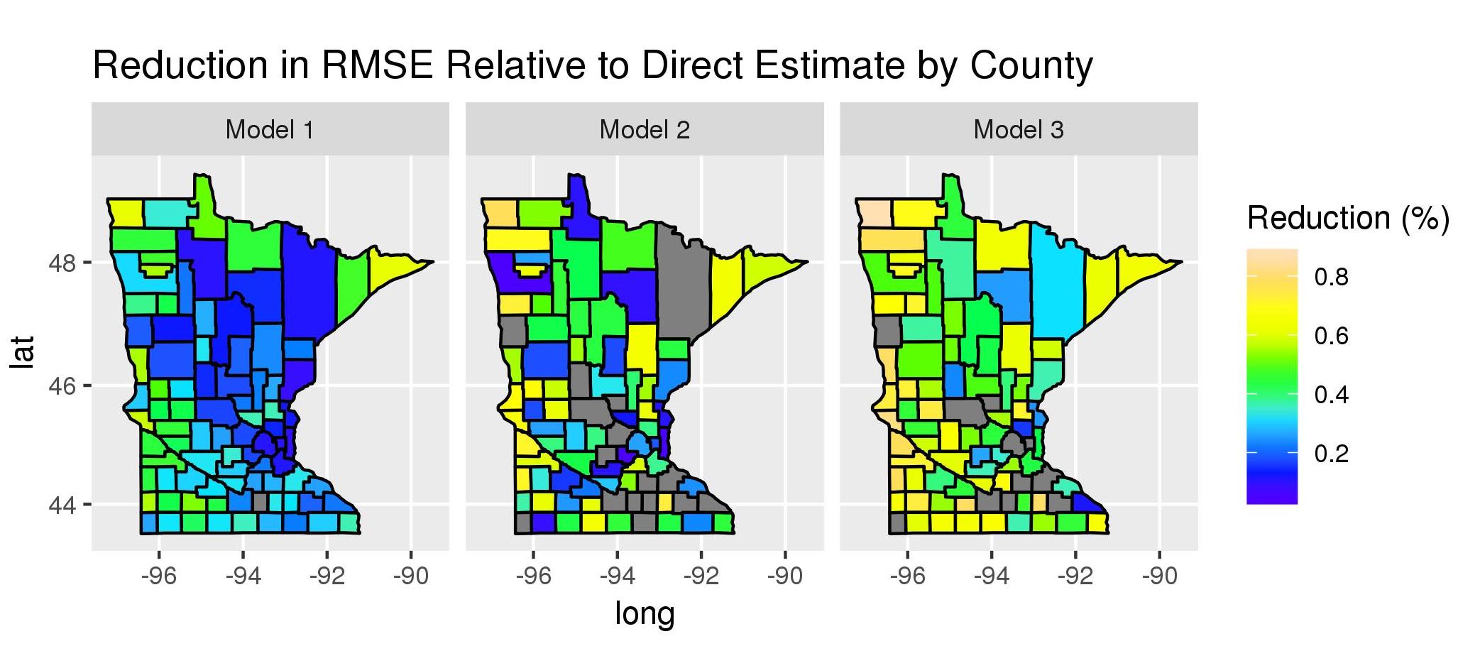
Figure 1: Model reduction in RMSE compared to the Direct estimates, averaged over 50 simulations. Counties that did not see a reduction are not plotted (shown in gray).

8 Poverty Estimate Data Analysis

The Small Area Income and Poverty Estimates program (SAIPE) is a U.S. Census Bureau program that produces estimates of median income and the number of people below the poverty threshold for states, counties, and school districts, as well as for various subgroups of the population. The SAIPE estimates are critical in order for the Department of Education to allocate Title I funds.

The current model used to generate SAIPE poverty estimates is an area-level Fay-Herriot model (Fay III and Herriot,, 1979) on the log scale. The response variable is the log transformed HT direct estimates from the single year ACS of the number of individuals in poverty at the county level. The model includes a number of powerful county level covariates such as the number of claimed exemptions from federal tax return data, the number of people participating in the Supplemental Nutrition Assistance Program (SNAP), and the number of Supplemental Security Income (SSI) recipients. Luery, (2011) provides a comprehensive overview of the SAIPE program, including the methodology used to produce various area-level estimates and the covariates used in the model.

We use a single year of ACS data (2014 again) from Minnesota to fit the three models described in Section 7. The model based estimators we present are not meant to replace the current SAIPE methodology, but rather to illustrate how unit-level models can be used in an informative sampling application such as this one. The model-based predictions of the proportion of people below the poverty threshold by county under each method are presented and compared with a direct estimator.

In Figure 2 we show the estimate of the proportion of people below the poverty level by county for each of the model-based estimators as well as the HT direct estimator. Note that a small amount of noise has been added to the HT direct estimates as a disclosure avoidance practice. All of the estimates here seem to capture the same general spatial trend. The model based estimates resemble smoothed versions of the direct estimates, especially in the more rural areas of the state. Small sample sizes can lead to direct estimates with high variance, but the model based approaches can “share information” across areas, which leads to more precise estimates. We also compare the reduction in model based standard errors when compared to the HT direct estimate in Figure 3. This illustrates the precision that is gained by using a model-based estimator rather than a direct estimator in a SAE setting. Model 3 in particular appears to have the lowest standard errors in more rural areas and Model 1 seems to have lower standard errors in more populated areas. For this particular application, all three of the models we explored would be valid choices, with substantial reductions in RMSE as shown in Section  7.

In this case, the population cell sizes were known, however in many applications they may not be, in which case Model 2 would likely be the best option. In other cases where incorporating covariate information is desired, Model 2 is not well equipped to make estimates. This application was conducted for a single state, however if one wanted to scale the analysis, for example making estimates for every county in the United States, Model 1 appears to be the most computationally efficient. An approach similar to Model 2, albeit using a different nonlinear regression approach from the Gaussian Process regression considered here, may also be computationally efficient. Vandendijck et al., (2016) reported strong results using splines for this setup. Overall we found that each of these unit-level methods can offer precise area-level estimates, however, the properties of the particular dataset under consideration as well as the goals of the user should drive which model is selected.

Modeling poverty counts at the unit level has a number of benefits when compared to area-level models. Specifically, the current SAIPE model is on the log scale, and thus cannot naturally accommodate estimates for areas with a corresponding direct estimate of zero, whereas unit-level modeling need not be on the log scale, and thus does not suffer from this problem. Additionally, making predictions at multiple spatial resolutions is straightforward in the unit-level setting, as predictions can be generated for all units in the population and then aggregated as necessary, i.e., the so-called bottom-up approach. Under a unit-level approach, one could generate poverty estimates at both a county level and school district level under the same model. In addition to these structural benefits, Table 1 illustrates that unit-level models have the capacity to provide substantial reductions in MSE and variance when compared to direct estimators.

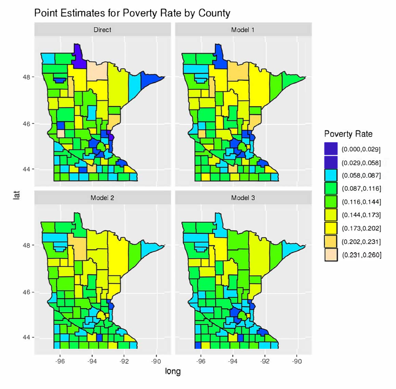
Figure 2: Noise infused HT direct and model based point estimates of poverty rate by county for Minnesota in 2014.

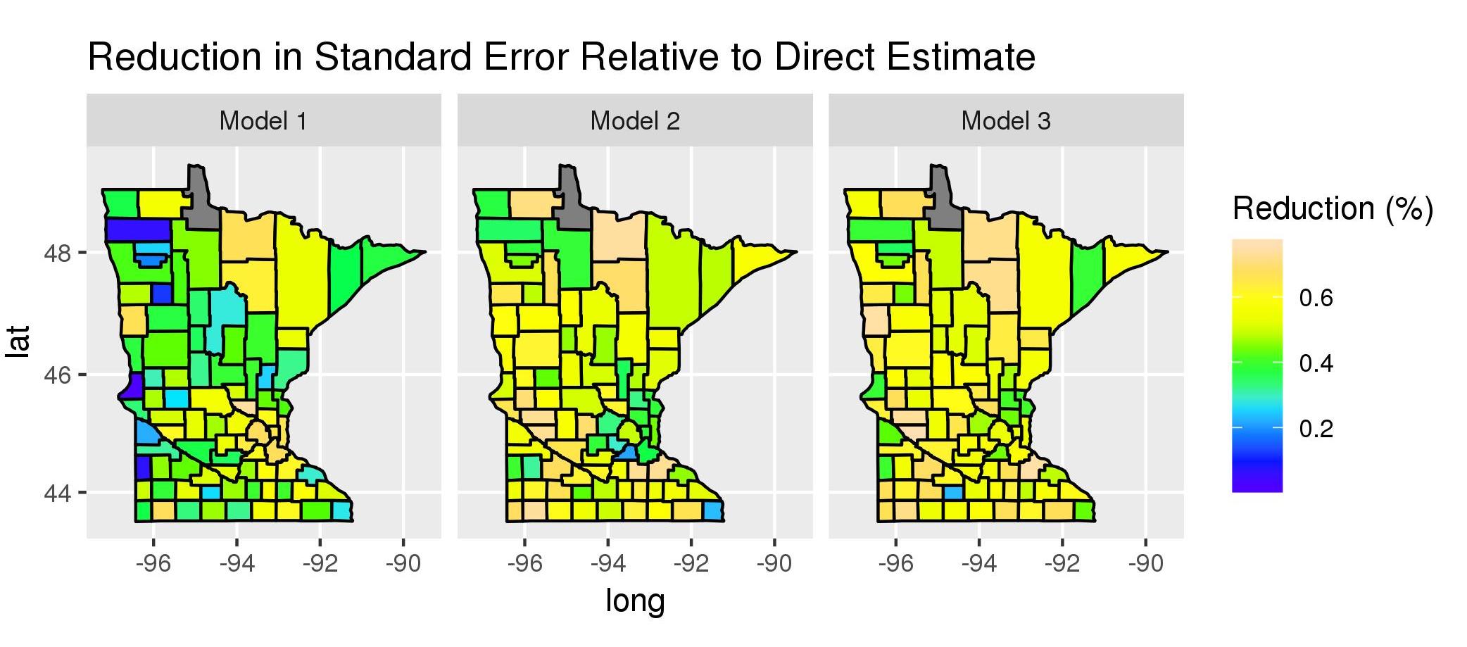
Figure 3: Model based reduction in standard errors for poverty rate by county. Counties that did not see a reduction are not plotted (shown in gray).

9 Conclusion

Through a comprehensive methodological review we have demonstrated that unit-level models pose many advantages relative to area-level models. These advantages include increased precision and straightforward spatial aggregation (the so-called benchmarking problem), among others. Estimation of unit-level models requires attention to the specific sampling design. That is, the unit response may be dependent on the probability of selection, even after conditioning on the design variables. In this sense, the sampling design is said to be informative and care must be taken in order to avoid bias.

In the context of small area estimation, we have described several strategies for unit-level modeling under informative sampling designs and illustrated their effectiveness relative to design-based estimators (direct estimates). Specifically, our simulation study (Section 7) illustrated three model-based estimators that exhibited superior performance relative to the direct estimator in terms of MSE, with Model 3 performing best in this regard. Among the three models compared in this simulation, Model 1 displayed the lowest computation time relative to the other model-based estimators and, therefore, may be advantageous in higher-dimensional settings.

The models in Section 7 (and Section 8) constitute modest extensions to models currently in the literature. Specifically, Model 2 provides an extension to Vandendijck et al., (2016), whereas Model 3 can be seen as a Bayesian version of the model proposed by Pfeffermann and Sverchkov, (2007). With these tools at hand, there are many opportunities for future research. For example, including administrative records into the previous model formulations constitutes one area of active research as care needs to be taken to probabilistically account for the record linkage. Methods for disclosure avoidance in unit-level models also provides another avenue for future research. In short, there are substantial opportunities for improving the models presented herein. In doing so, the aim is to provide computationally efficient estimates with improved precision. Ultimately, this will provide additional tools for official statistical agencies, survey methodologists, and subject-matter scientists.

References

- Asparouhov, (2006) Asparouhov, T. (2006). “General multi-level modeling with sampling weights.” Communications in Statistics—Theory and Methods, 35, 3, 439–460.
- Battese et al., (1988) Battese, G. E., Harter, R. M., and Fuller, W. A. (1988). “An error-components model for prediction of county crop areas using survey and satellite data.” Journal of the American Statistical Association, 83, 401, 28–36.
- Bauder et al., (2018) Bauder, M., Luery, D., and Szelepka, S. (2018). “Small area estimation of health insurance coverage in 2010 – 2016.” Tech. rep., Small Area Methods Branch, Social, Economic, and Housing Statistics Division, U. S. Census Bureau.
- Beaumont, (2008) Beaumont, J.-F. (2008). “A new approach to weighting and inference in sample surveys.” Biometrika, 95, 3, 539–553.
- Besag, (1974) Besag, J. (1974). “Spatial interaction and the statistical analysis of lattice systems (with discussion).” Journal of the Royal Statistical Society. Series B, 36, 192 – 236.
- Binder, (1983) Binder, D. A. (1983). “On the variances of asymptotically normal estimators from complex surveys.” International Statistical Review, 51, 3, 279–292.
- Binder and Patak, (1994) Binder, D. A. and Patak, Z. (1994). “Use of estimating functions for estimation from complex surveys.” Journal of the American Statistical Association, 89, 427, 1035–1043.
- Carpenter et al., (2017) Carpenter, B., Gelman, A., Hoffman, M. D., Lee, D., Goodrich, B., Betancourt, M., Brubaker, M., Guo, J., Li, P., and Riddell, A. (2017). “Stan: A probabilistic programming language.” Journal of Statistical Software, 76, 1.
- Chen et al., (2014) Chen, C., Wakefield, J., and Lumely, T. (2014). “The use of sampling weights in Bayesian hierarchical models for small area estimation.” Spatial and Spatio-temporal Epidemiology, 11, 33–43.
- Congdon and Lloyd, (2010) Congdon, P. and Lloyd, P. (2010). “Estimating small area diabetes prevalence in the US using the behavioral risk factor surveillance system.” Journal of Data Science, 8, 2, 235–252.
- Dong et al., (2014) Dong, Q., Elliott, M. R., and Raghunathan, T. E. (2014). “A nonparametric method to generate synthetic populations to adjust for complex sampling design features.” Survey Methodology, 40, 1, 29–46.
- Fay III and Herriot, (1979) Fay III, R. E. and Herriot, R. A. (1979). “Estimates of income for small places: an application of James-Stein procedures to census data.” Journal of the American Statistical Association, 74, 366a, 269–277.
- Franco and Bell, (2014) Franco, C. and Bell, W. R. (2014). “Borrowing information overtime in binomial/logit normal models for small area estimation.” Statistics in Transition, 16, 563 – 584.
- Gelman, (2007) Gelman, A. (2007). “Struggles with survey weighting and regression modeling.” Statistical Science, 22, 2, 153–164.
- Gelman et al., (1995) Gelman, A., Carlin, J. B., Stern, H. S., and Rubin, D. B. (1995). Bayesian Data Analysis. London: Chapman and Hall.
- Gelman and Little, (1997) Gelman, A. and Little, T. C. (1997). “Poststratification into many categories using hierarchical logistic regression.”
- Grilli and Pratesi, (2004) Grilli, L. and Pratesi, M. (2004). “Weighted estimation in multilevel ordinal and binary models in the presence of informative sampling designs.” Survey Methodology, 30, 1, 93–103.
- Guadarrama et al., (2018) Guadarrama, M., Molina, I., and Rao, J. N. K. (2018). “Small area estimation of general parameters under complex sampling designs.” Computational Statistics and Data Analysis, 121, 20 – 40.
- Hidiroglou and You, (2016) Hidiroglou, M. A. and You, Y. (2016). “Comparison of unit level and area level small area estimators.” Survey Methodology, 42, 41–61.
- Jiang and Lahiri, (2006) Jiang, J. and Lahiri, P. (2006). “Estimation of finite population domain means: A model-assisted empirical best prediction approach.” Journal of the American Statistical Association, 101, 473, 301–311.
- Kim, (2002) Kim, D. H. (2002). “Bayesian and empirical Bayesian analysis under informative sampling.” Sankhyā: The Indian Journal of Statistics, Series B, 64, 3, 267–288.
- Kim et al., (2017) Kim, J. K., Park, S., and Lee, Y. (2017). “Statistical inference using generalized linear mixed models under informative cluster sampling.” Canadian Journal of Statistics, 45, 4, 479–497.
- Kish, (1965) Kish, L. (1965). Survey Sampling. New York: Wiley.
- Kish, (1992) — (1992). “Weighting for unequal Pi.” Journal of Official Statistics, 8, 2, 183.
- Korn and Graubard, (2003) Korn, E. L. and Graubard, B. I. (2003). “Estimating variance components by using survey data.” Journal of the Royal Statistical Society: Series B (Statistical Methodology), 65, 1, 175–190.
- Little, (1993) Little, R. J. (1993). “Post-stratification: a modeler’s perspective.” Journal of the American Statistical Association, 88, 423, 1001–1012.
- Little, (2012) — (2012). “Calibrated Bayes, an alternative inferential paradigm for official statistics.” Journal of Official Statistics, 28, 3, 309.
- Luery, (2011) Luery, D. M. (2011). “Small area income and poverty estimates program.” In Proceedings of 27th SCORUS Conference, 93–107.
- Lumley et al., (2017) Lumley, T., Scott, A., et al. (2017). “Fitting regression models to survey data.” Statistical Science, 32, 2, 265–278.
- Malec et al., (1999) Malec, D., Davis, W. W., and Cao, X. (1999). “Model-based small area estimates of overweight prevalence using sample selection adjustment.” Statistics in Medicine, 18, 23, 3189–3200.
- Malec et al., (1997) Malec, D., Sedransk, J., Moriarity, C. L., and LeClere, F. B. (1997). “Small area inference for binary variables in the National Health Interview Survey.” Journal of the American Statistical Association, 92, 439, 815–826.
- Midzuno, (1951) Midzuno, H. (1951). “On the sampling system with probability proportionate to sum of sizes.” Annals of the Institute of Statistical Mathematics, 3, 1, 99–107.
- Molina et al., (2014) Molina, I., Nandram, B., and Rao, J. (2014). “Small area estimation of general parameters with application to poverty indicators: a hierarchical Bayes approach.” The Annals of Applied Statistics, 8, 2, 852–885.
- Nathan and Holt, (1980) Nathan, G. and Holt, D. (1980). “The effect of survey design on regression analysis.” Journal of the Royal Statistical Society: Series B (Statistical Methodology), 42, 3, 377–386.