Solving fermion problems without solving the sign problem: symmetry-breaking wave functions from similarity-transformed propagators for solving 2D quantum dots

Abstract

It is well known that the use of the primitive second-order propagator in Path Integral Monte Carlo calculations of many-fermion systems leads to the sign problem. In this work, we show that by using the similarity-transformed Fokker-Planck propagator, it is possible to solve for the ground state of a large quantum dot, with up to 100 polarized electrons, without solving the sign problem. These similarity-transformed propagators naturally produce rotational symmetry-breaking ground state wave functions previously used in the study of quantum dots and quantum Hall effects. However, instead of localizing the electrons at positions which minimize the potential energy, this derivation shows that they should be located at positions which maximize the bosonic ground state wave function. Further improvements in the energy can be obtained by using these as initial wave functions in a Ground State Path-Integral Monte Carlo calculation with second and fourth-order propagators.

I Introduction

Two dimensional, circular parabolically confined quantum dots, are not only physical systems of great experimental interestsrei02 , but are also mathematical models par excellence for the numerical study of the many-fermion problem. In constrast to real atoms, where the hydrogen atom’s partition function is divergentbli95 , these “Hooke’s atoms”nei62 only have bound states, with convergent partition functions. This lack of additional complications allows us to focus attention solely on the effect of interaction and Fermi statistics. In this work we compute the ground state energy of up to $N=100$ spin-polarized electrons, applicable to the study of quantum dots under strong magentic fields.

Quantum dots have been extensively studied by traditional methods of quantum many-body theory, such as Hartree-Fock (HF)yan99 , Density Functional Theory (DFT)fer94 ; hir99 , Configuration Interaction (CI)ron06 , Coupled-Cluster (CC)ped ; wal , Variational Monte Carlo (VMC)har02 ; kai02 , Diffusion Monte Carlo (DMC)ped ; ped03 ; gho07 and Path Integral Monte Carlo (PIMC)mak98 ; egg99 ; egg00 ; reu03 ; chin15 ; ilk17 , with varying degrees of accuracy. However, with increasing number of electrons (say $N\!>$10), basis-function based methods, such as CI and CC, simply cannot keep up with the exponential growth of needed basis functions. For $N>20$, even VMC and DMC have difficulties in constructing a good trial wave function involving many excited states. In principle, since PIMC does not require an initial trial wave function, it can be used to treat large quantum dots. However, PIMC can only extract the ground state at large imaginary time, and if many short-time anti-symmtric propagators are used, then the resulting sign-problem will overwhelm the ground state signal. One can side-step the sign problem in DMC and PIMC by invoking the fixed-node or the restricted-path approximationilk17 ; cep95 . These approximations have worked surprising well and currently the ground state energy of the largest spin-balanced quantum dot with $N=60$ has been obtained using PIMCilk17 . Here, we proposes a new way of solving the fermion problem in large quantum dots without invoking any prior assumptions.

In Ref.chin15 , it was suggested that fourth-order propagators can be used in PIMC to reduce the number of anti-symmtric propagators used and thereby reduce the serverity of the sign problem. This is indeed a workable scheme for up to $N\approx$ 30. However, beyond that, the sign problem remains severe at large imaginary time.

In this work, we overcome this fundamental problem by reducing the length of the imaginary time needed by doing PIMC on symmetry-breaking wave functions that are already very close to the ground state, that is, we apply a Fermion Ground State Path Integral Monte Carlo (FGSPIMC) method to quantum dots. While the bosonic GSPIMC method is well knowncep95 ; sar00 , the fermionic version has only been tried previously in the context of shadow wave functioncal14 .

To derive such a symmetry-breaking wave function, we first derive, from a new perspective, some basic results on similarity transformed propagators in Section II. In Section III, we show that the harmonic oscillator has the remarkable property that if its propagator is similarity-transformed by its ground state wave function, the resulting Fokker-Planck propagator, even if only approximated to first order, yields the exact partition function of the harmonic oscillator. We show in Section IV that, when these Fokker-Planck propagators are anti-symmetrized in the many-fermion case, they yielded the exact ground state energies of non-interacting fermions in a harmonic oscillator. That is, a many-fermion problem has been solved exactly without knowing the exact propagator, the exact wave functions, or having to solve any sign problem. In Section V, we show that in the presence of pair-wise repulsive Coulomb interactions, the resulting Fokker-Planck propagator naturally produces spontaneous symmetry-breaking (SSB) wave functions previously used in the studies of quantum dots and quantum Hall effectsyan99 ; mik01 ; yan02 ; yan07 . For quantum dots, we show that a variational version of these SSB wave functions can already yield energies to within 1$\%$ of the best ground state energies. In Section VI, we show that this remaining 1$\%$ can be recovered by doing a FGSPIMC calculation using a fourth-order propagator. In Section VII, we summarize our conclusions and suggest furture applications of this work.

II Similarity transformed propagators

For completeness, we will derive here some basic results in a new way. Let the imaginary-time propagator (or density matrix) of the Hamiltonian operator $H$ be

$$G({\bf x},{\bf x}^{\prime};\tau)=\langle{\bf x}|{\rm e}^{-\tau H}|{\bf x}^{\prime}\rangle,$$ (1)

then corresponding partition function

$$Z(\tau)=\int d{\bf x}\,G({\bf x},{\bf x};\tau)$$ (2)

is invariant under the similarity transformation

$$Z(\tau)=\int d{\bf x}\langle{\bf x}|\phi{\rm e}^{-\tau H}\phi^{-1}|{\bf x}\rangle=\int d{\bf x}\phi({\bf x})G({\bf x},{\bf x};\tau)\phi^{-1}({\bf x})=\int d{\bf x}\,G({\bf x},{\bf x};\tau),$$

provided that $\phi({\bf x})$ is a non-vanishing real function at all ${\bf x}$,

$$\phi({\bf x})\neq 0.$$ (3)

Therefore, $Z(\tau)$ can also be computed from the transformed propagator

$$\tilde{G}({\bf x},{\bf x}^{\prime};\tau)=\langle{\bf x}|{\rm e}^{-\tau\tilde{H}}|{\bf x}^{\prime}\rangle$$

corresponding to the transformed Hamiltonian

$$\tilde{H}=\phi({\bf x})H\phi^{-1}({\bf x}).$$ (4)

Since $\phi({\bf x})$ is non-vanishing everywhere, it can always be written as

$$\phi({\bf x})=e^{-S({\bf x})},$$ (5)

which defines $S({\bf x})$. We will call $S({\bf x})$ the action of the wave function. For a single-particle Hamiltonian in $D$-dimension of the separable form,

$$H=-\frac{1}{2}\nabla^{2}+V({\bf x})=K+V({\bf x}),$$

the transformed Hamiltonian is

$$\tilde{H}={\rm e}^{-S({\bf x})}K{\rm e}^{S({\bf x})}+V({\bf x}).$$

Since $K$ is only a second-order derivative operator, the general operator identity

$${\rm e}^{C}K{\rm e}^{-C}=K+[C,K]+\frac{1}{2!}[C,[C,K]]+\frac{1}{3!}[C,[C,[C,K]]]+\cdots,$$ (6)

with $C=-S(x)$, terminates at the double commutator term:

$${\rm e}^{-S({\bf x})}K{\rm e}^{S({\bf x})}=K-[S,K]+\frac{1}{2}[S,[S,K]].$$

From the definition of $K=-\frac{1}{2}\nabla^{2}$, one has

$$[S,K]=\nabla S\cdot\nabla+\frac{1}{2}\nabla^{2}S,\qquad[S,[S,K]=-(\nabla S)^{2}$$

and therefore the transformed Hamiltonian is

$$\tilde{H}\psi = (K+D+E_{L})\psi$$

where $D$ is the drift operator

$$D\psi=\nabla\cdot\Bigl{(}{\bf v}({\bf x})\psi\Bigr{)}$$

with drift velocity ${\bf v}({\bf x})=-\nabla S({\bf x})$ and

$$E_{L}({\bf x})=\frac{1}{2}\nabla^{2}S-\frac{1}{2}(\nabla S)^{2}+V=\frac{H\phi({\bf x})}{\phi({\bf x})}$$

is the local energy function. The transformed imaginary time propagator is then

$$\tilde{G}({\bf x},{\bf x}^{\prime};\tau)=\langle{\bf x}|{\rm e}^{-\tau(K+D+E_{L})}|{\bf x}^{\prime}\rangle.$$ (7)

The present derivation of this fundamental result on the basis of (6) is new, as far as the author can tell.

If $E_{L}$ is a constant, then because of the non-vanishing condition (3), $\phi({\bf x})$ must be the bosonic ground state $\psi_{0}({\bf x})$ of $H$. In this case, (7) is the Fokker-Planck (FP) propagator whose long time stationary solution is the square of the ground state wave function: $\phi^{2}({\bf x})=\psi_{0}^{2}({\bf x})$.

Even in cases where $E_{L}$ is not a constant, the advantage of using the transformed propagator (7) is that low order approximates of $\tilde{G}({\bf x},{\bf x}^{\prime};\tau)$ can be far more accurate than low order approximates of $G({\bf x},{\bf x}^{\prime};\tau)$. For example, a first-order (in $\tau$) approximation of (7) is

$$\tilde{G}_{1}({\bf x},{\bf x}^{\prime};\tau)=\langle{\bf x}|{\rm e}^{-\tau K}{\rm e}^{-\tau D}|{\bf x}^{\prime}\rangle{\rm e}^{-\tau E_{L}({\bf x})}.$$ (8)

Since as shown in Ref.chin90 ,

$$\langle{\bf x}|{\rm e}^{-\tau K}|{\bf x}_{1}\rangle = (2\pi\tau)^{-D/2}\exp\left[-\frac{1}{2\tau}({\bf x}-{\bf x}_{1})^{2}\right],$$

$$\langle{\bf x}_{1}|{\rm e}^{-\tau D}|{\bf x}_{0}\rangle = \delta[{\bf x}_{1}-{\bf x}(\tau)],$$

where ${\bf x}(\tau)$ is the solution to the drift equation with initial position ${\bf x}_{0}$:

$$\frac{d{\bf x}}{d\tau}={\bf v}({\bf x})=-\nabla S({\bf x}),$$

the resulting first-order propagator is

$$\tilde{G}_{1}({\bf x},{\bf x}_{0};\tau) = \int d{\bf x}_{1}\langle{\bf x}|{\rm e}^{-\tau K}|{\bf x}_{1}\rangle\langle{\bf x}_{1}|{\rm e}^{-\tau D}|{\bf x}_{0}\rangle{\rm e}^{-\tau E_{L}({\bf x}_{0})}$$ (9)

$$= \frac{1}{(2\pi\tau)^{D/2}}\exp\left[-\frac{1}{2\tau}({\bf x}-{\bf x}(\tau))^{2}\right]{\rm e}^{-\tau E_{L}({\bf x}_{0})}.$$

This is to be compared with the first-order approximation of $G({\bf x},{\bf x}_{0};\tau)$:

$$G_{1}({\bf x},{\bf x}_{0};\tau) = \int d{\bf x}_{1}\langle{\bf x}|{\rm e}^{-\tau K}{\rm e}^{-\tau V}|{\bf x}_{0}\rangle$$ (10)

$$= \frac{1}{(2\pi\tau)^{D/2}}\exp\left[-\frac{1}{2\tau}({\bf x}-{\bf x}_{0})^{2}\right]{\rm e}^{-\tau V({\bf x}_{0})}.$$

The transformed propagator (9) resplaces the bare potential $V({\bf x})$, which can be highly singular, by $E_{L}({\bf x})$, which can be a non-singular and less fluctuating. It also replaces the aimless Gaussian random walk in $G_{1}({\bf x},{\bf x}_{0};\tau)$ by Gaussian random walks along trajectories of the velocity field ${\bf v}({\bf x})=-\nabla S({\bf x})$ produced by the trial wave function. This transformed propagator $\tilde{G}_{1}({\bf x},{\bf x}_{0};\tau)$ is the basis for doing DMCmos82 ; rey82 with importance-sampling and is the generalized Feynman-Kac path integralcaf88 when $\phi({\bf x})\neq\psi_{0}({\bf x})$. In the next section, we will show that this FP propagator produces a remarkable result for the harmonic oscillator.

III Transformed harmonic propagators

Consider a $D$-dimensional harmonic Hamiltonian with energy in units of $\hbar\omega$ and length in units of $\sqrt{\hbar/m\omega}$,

$$H=-\frac{1}{2}\nabla^{2}+\frac{1}{2}{\bf x}^{2}.$$

In this case, one can take $\phi({\bf x})=\psi_{0}({\bf x})$, the exact ground state wave function with action

$$S({\bf x})=\frac{1}{2}{\bf x}^{2},$$

and a constant $E_{L}$,

$$E_{L} = \frac{1}{2}\nabla^{2}S-\frac{1}{2}(\nabla S)^{2}+\frac{1}{2}{\bf x}^{2}=\frac{D}{2}\equiv E_{0},$$ (11)

which is the exact ground state energy.

The solution ${\bf x}(\tau)$ to the drift equation with initial position ${\bf x}_{0}$ is then simply

$$\frac{d{\bf x}}{d\tau}={\bf v}({\bf x})=-\nabla S({\bf x})=-{\bf x}\quad\rightarrow\quad{\bf x}(\tau)={\bf x}_{0}{\rm e}^{-\tau},$$

giving the first-order transformed propagator (9):

$$\tilde{G}_{1}({\bf x},{\bf x}_{0};\tau) = \frac{1}{(2\pi\tau)^{D/2}}\exp\left[-\frac{1}{2\tau}({\bf x}-{\bf x}_{0}{\rm e}^{-\tau})^{2}\right]{\rm e}^{-\tau E_{L}}.$$ (12)

This is to be compared to the exact FK propagator, corresponding to the Ornstein-Uhlenbeckuhl process:

$$\tilde{G}({\bf x},{\bf x}_{0};\tau)=\frac{1}{[2\pi T(\tau)]^{D/2}}\exp\left[-\frac{1}{2T(\tau)}({\bf x}-{\bf x}_{0}{\rm e}^{-\tau})^{2}\right]{\rm e}^{-\tau E_{L}}$$ (13)

with

$$T(\tau)=\frac{1}{2}(1-{\rm e}^{-2\tau}).$$ (14)

In the limit of $\tau\rightarrow\infty$, this exact FK propagator correctly gives

$$\tilde{G}({\bf x},{\bf x}_{0};\tau)\rightarrow\frac{1}{\pi^{D/2}}\exp\left[-{\bf x}^{2}\right]{\rm e}^{-\tau E_{0}}=\psi^{2}_{0}({\bf x}){\rm e}^{-\tau E_{0}},$$ (15)

which is proportional to the square of the ground state wave function. By contrast, the first-order transformed propagator $\tilde{G}_{1}({\bf x},{\bf x}_{0};\tau)\rightarrow 0$ as $\tau\rightarrow\infty$ and bears no resemblance to any wave function. This seems to be a very poor approximation to the exact propagator. However, if one computes the partition function from this single transformed propagator,

$$Z = \int d{\bf x}\tilde{G}_{1}({\bf x},{\bf x};\tau)=\frac{1}{(2\pi\tau)^{D/2}}\int d{\bf x}\exp\left[-\frac{1}{2\tau}{\bf x}^{2}(1-{\rm e}^{-\tau})^{2}\right]{\rm e}^{-\tau E_{L}}$$ (16)

$$= \frac{1}{(2\pi\tau)^{D/2}}[2\pi\tau(1-{\rm e}^{-\tau})^{-2}]^{D/2}{\rm e}^{-\tau D/2}=\left(\frac{{\rm e}^{-\frac{1}{2}\tau}}{1-{\rm e}^{-\tau}}\right)^{D}=[2\sinh(\tau/2)]^{-D},$$ (17)

the result is exactly correct. That is, when the exact ground state wave function, which knows nothing about $\tau$, is used to derived the transformed propagator, the resulting single bead calculation produces the correct $Z(\tau)$ at all $\tau$, i.e., at all temperature!

The only difference between the transformed first-order propagator (12) and the exact FK propagator (13) is that the variance of the Gaussian distribution is $\tau$ rather than $T(\tau)$. This single bead calculation of $Z(\tau)$ is exact because the variance of the Gaussian distribution, after doing the integral, is cancelled by the initial normalization constant and the integral is actually independent of the variance. This suggests that the solution to the drift equation, which is purely classical, is of unexpected importance for understanding quantum statistical dynamics, at least for the harmonic oscillator. In the next Section, we will see how the drift term exactly solves the problem of many non-interacting fermions in a harmonic oscillator, without knowing the exact harmonic oscillator propagator.

IV Non-interacting fermions in a harmonic oscillator

In (15), one sees that the exact FP propagator yields the square of the ground state wave function in the limite of $\tau\rightarrow\infty$ with

$${\bf x}(\tau)\rightarrow 0\quad{\rm and}\quad T(\tau)\rightarrow\frac{1}{2}.$$

In the first-order transformed propagator (12), one also has ${\bf x}(\tau)\rightarrow 0$ as $\tau\rightarrow\infty$. What is left is then a Gaussian distribution with variance $\tau$. If one now regards this variance $\tau$ as just a variational parameter, and dissociate it from being the imaginary time needed to be set to infinity, then the choice of $\tau=1$ would give the correct ground state wave function (but not its square). This seems to be a rather contrived way of obtaining the ground state wave function from the transformed propagator, but its utility is the following.

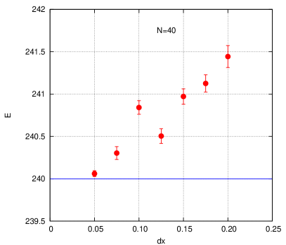
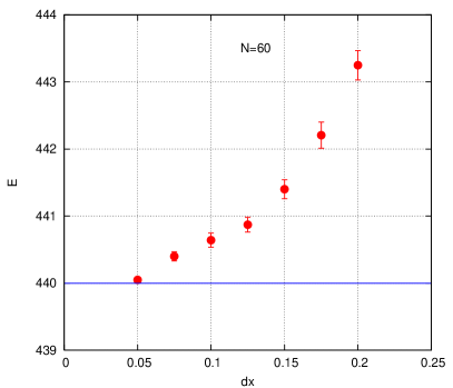
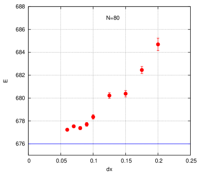
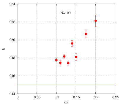
Figure 1: (color online) The energy of $N$ non-interacting, spin-polarized fermions in a 2D harmonic oscillator. For $N=40,60,80,100$, the exact energies, indicated by the horizontal blue line, are 240, 440, 676 and 945 (in unit of $\hbar\omega$) respectively. The calculated lowest energies, at or near the smallest value of $\Delta x$, are 240.06(4), 440.05(3), 677.2(1) and 947.4(2) respectively.

Consider $N$ non-interacting particles in a $D$-dimensional harmonics oscillator. According to the above discussion, each particle’s ground state wave function would be (unnormalized)

$$\psi_{0}({\bf x}_{i})=\exp[-\frac{1}{2\tau}({\bf x}_{i}-{\bf s}_{i})^{2}]$$

with $\tau=1$ and where ${\bf s}_{i}={\bf x}(\tau\rightarrow\infty)\rightarrow 0$. However, for our purpose of anti-symmetrization, we will only let each ${\bf s}_{i}$ approaches close to zero, but not exactly zero. For $N$ spin-polarized fermions, as long as all ${\bf s}_{i}$ are distinct, one can construction the anti-symmetric determinant wave function

$$\Psi({\bf x}_{1},{\bf x}_{2}\dots{\bf x}_{N})=\det\Bigl{|}\exp[-\frac{1}{2}({\bf x}_{i}-{\bf s}_{j})^{2}]\Bigr{|}.$$ (18)

Remarkably, this simple wave function gives the exact energy of $N$ non-interacting fermions in a harmonic oscillator so long as all ${\bf s}_{i}$ are close to zero but remain distinct from one another. For the case of $D=2$, this is shown in Fig.1.

These four calculations were done by generating $N$ positions of ${\bf s}_{i}$ randomly near the origin with approximate separations of $\Delta x$. This is necessary to prevent ${\bf s}_{i}$ from overlapping, causing the determinant to vanish. The square of this wave function (no sign problem) is then sampled using the Metropolis et al.met algorithm. To compute the energy, it is necessary to compute the inverse of the matrix in (18). With decreasing $\Delta x$, particles are closer to each other and closer to the origin. For $N$ up to 60, one sees that the calculation gives the correct energy up to statistical uncertainties. For $N>60$, there is a systematic bias due the limitation of double precision in Fortran. When $N$ is large, the determinant is nearly vanishing and the routine for inverting the matrix is increasingly inaccurate. This prevents the calculation from being done at a $\Delta x$ sufficiently small to give the correct result. This is shown in the case of $N=80$ and $N=100$. The use of multiple-precision arithematics would alleviate this purely numerical problem.

This wave function (18) for computing the non-interacting fermion energy is much simpler than anti-symmetrizing excited states of the harmonic oscillator, or using the exact harmonic oscillator propagatorchin15 . The reason why this wave function (18) is exact can be seen from formulas given in Ref.mik01 ; yan02 . Here, we can give a simple example to illustrate the idea. For $N=2$, the (unnormalize) antisymmetrized wave function is

$$\Psi({\bf x}_{1},{\bf x}_{2}) = {\rm e}^{-\frac{1}{2}[({\bf x}_{1}-{\bf s}_{1})^{2}+({\bf x}_{2}-{\bf s}_{2})^{2}]}-{\rm e}^{-\frac{1}{2}[({\bf x}_{1}-{\bf s}_{2})^{2}+({\bf x}_{2}-{\bf s}_{1})^{2}]}$$ (19)

$$= {\rm e}^{-\frac{1}{2}[({\bf x}_{1}-{\bf s}_{1})^{2}+({\bf x}_{2}-{\bf s}_{2})^{2}]}(1-{\rm e}^{-[({\bf s}_{1}-{\bf s}_{2})\cdot({\bf x}_{1}-{\bf x}_{2})]}).$$

In the limit of ${\bf s}_{i}\rightarrow 0$, the wave function to first-order in ${\bf s}_{1},{\bf s}_{2}$ is just

$$\Psi({\bf x}_{1},{\bf x}_{2})=({\bf s}_{1}-{\bf s}_{2})\cdot({\bf x}_{1}-{\bf x}_{2})e^{-\frac{1}{2\tau}({\bf x}_{1}^{2}+{\bf x}_{2}^{2})},$$ (20)

which is proportional to the correct two fermion wave function in the harmonic oscillator. Note that we must have ${\bf s}_{1}\neq{\bf s}_{2}$, otherwise the wave function vanishes.

V Spontaneous symmetry-breaking wave functions

From this point onward, we will only discuss the case of $D=2$. For $N$ fermions in a harmonic oscillator with Coulomb interactions, the Hamiltonian is given bygho07

$$H=-\frac{1}{2}\sum_{i=1}^{N}\nabla_{i}^{2}+\frac{1}{2}\sum_{i=1}^{N}{\bf x}_{i}^{2}+\sum_{i>j}\frac{{\lambda}}{x_{ij}}.$$ (21)

where $x_{ij}=|{\bf x}_{i}-{\bf x}_{j}|$. The similarily transformed propagator will yield the corresponding anti-symmetric wave function

$$\Psi_{D}({\bf x}_{1},{\bf x}_{2}\dots{\bf x}_{N})=\det\Bigl{|}\exp[-\frac{1}{2\tau}({\bf x}_{i}-{\bf s}_{j})^{2}]\Bigr{|}.$$ (22)

Here, we will let the variance of the Gaussian distribution, $\tau$, usually set to 1, be allowed to vary. As before, each ${\bf s}_{i}={\bf x}_{i}(\tau\rightarrow\infty)$ is a stationary point of the trajectory ${\bf x}_{i}(\tau)$ obeying the drift equation

$$\frac{d{\bf x}_{i}}{d\tau}=-\nabla_{i}S({\bf x}_{1},{\bf x}_{2}\dots,{\bf x}_{N}),$$ (23)

with $S({\bf x}_{1},{\bf x}_{2}\dots,{\bf x}_{N})$ being the action of the many-particle bosonic ground state wave function:

$$\Psi_{B}({\bf x}_{1},{\bf x}_{2}\dots{\bf x}_{N})={\rm e}^{-S({\bf x}_{1},{\bf x}_{2}\dots,{\bf x}_{N})}.$$

Note that the set of stationary points satisfying $d{\bf x}_{i}/d\tau=0$ correspond to $\nabla_{i}S(\{{\bf x}_{i}\})=0$, and are positions which minimize $S(\{{\bf x}_{i}\})$, or maximize the bosonic wave function. (The case of multiple local maxima will be discuss in later Sections.) In the non-interacting case, we have seen in the previous section that anti-symmetrizing the exact bosonic ground state produces the exact fermionic ground state.

With the added Coulomb interaction, the exact bosonic ground state is known only for two particles at coupling ${\lambda}=1$ with

$$S({\bf x}_{1},\dots{\bf x}_{N})=\frac{1}{2}\sum_{i=1}^{2}{\bf x}^{2}_{i}-\ln(1+x_{12}),$$ (24)

and $E_{0}=3$. The drift equations from (23) are then

$$\frac{d{\bf x}_{1}}{d\tau}=-{\bf x}_{1}+\frac{\hat{\bf x}_{12}}{1+x_{12}},\qquad\frac{d{\bf x}_{2}}{d\tau}=-{\bf x}_{2}+\frac{\hat{\bf x}_{21}}{1+x_{12}},$$

$$\rightarrow\quad\frac{d{\bf x}_{cm}}{d\tau}=-{\bf x}_{cm},\quad{\rm and}\quad\frac{d{\bf x}_{12}}{d\tau}=-{\bf x}_{12}+\frac{2\hat{\bf x}_{12}}{1+x_{12}}.$$

Since the drift equations are just first-order differential equations, they can be solved easily by any numerical method to arrive at their statinary points. In the above case, the stationary points can be gotten simply by setting the $\tau$-derivatives to zero:

$${\bf s}_{cm}=0\quad{\rm and}\quad{\bf s}_{12}=\hat{\bf x}_{12}(0)\quad\rightarrow\quad{\bf s}_{1}=\frac{1}{2}\hat{\bf x}_{12}(0),\quad{\bf s}_{2}=-\frac{1}{2}\hat{\bf x}_{12}(0).$$

The two stationary points ${\bf s}_{1}$ and ${\bf s}_{2}$ are antipodal points on a circle of radius $R=1/2$, oriented by the initial vector $\hat{\bf x}_{12}(0)$, which is entirely arbitrary. Thus any two such antipodal points on the circle can be stationary points of the above drift equation. However, when a specific pair of points is inserted into the fermion wave function (22), the resulting wave function no longer respects the rotational symmetry of the original Hamiltonian. Thus the transformed propagator naturally produces a spontaneous symmetry-breaking wave function, which has been extensively discussed in the literatureyan99 ; mik01 ; yan02 , notably by Yannouleas and Landmanyan99 ; yan02 ; yan07 . In these earlier discussions, such a wave function was simply viewed as an ansatz, and it is therefore entirely reasonable to take $\{{\bf s}_{i}\}$ as particle positions which minimize the classical potential energymik01 ; yan02 ; kai02 . In this case, they would be antipodal points on a circle with $R=2^{1/3}/2=0.62996$. Here, our derivation of this wave function from the transformed propagator showed that these stationary points are to be determined by the maximum of the bosonic wave function. In Fig.2 we compare the energies computed from the fermion wave function (22) using these two sets of stationary points with that from a 5-bead fermion PIMC calculation using an optimized fourth-order propagator, as described in Ref.chin15 . The top line gives the energy from using stationary points minimizing the potential energy. The bottom line gives the energy from using stationary points maximizing the bosonic wave function. This comparison clearly shows that one should use stationary points from the latter rather than from the former. Moreover, the fermion wave function (22) is optimal with $R=1/2$; any other radius yields a higher energy.

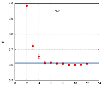
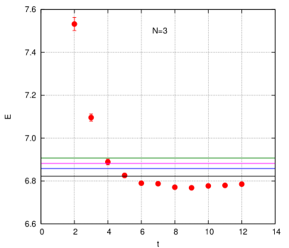
Figure 2: (color online) Left: Two-fermion energies at coupling ${\lambda}=1$. Symbols are results from a 5-bead PIMC calculation using an optimized fourth-order fermion propagatorchin15 yielding a minimum energy of 3.600(4) at imaginary time $t=10$. The top and the bottom line denote energy 3.6171(6) and 3.6085(5) respectively. See text for detail. Right: Three-fermion energies at coupling ${\lambda}=1$. Symbols show the 5-bead PIMC energy of 6.768(4) at $t=9$. From the top down, the four horizontal lines are three-fermion energies of 6.907(1), 6.882(1), 6.858(1), 6.822(1) respectively, computed from various forms of the wave function (22). See text for detail.

The rotational symmetry of this wave function can be restored by integrating over the angle of $\hat{\bf x}_{12}(0)$, bascially summing the wave function over all antipodal points on the circle. Such a symmetry-restored wave functionyan02 ; yan07 should have lower energy and may account for the difference of $0.0085(5)$ between this wave function’s energy and that of PIMC. In this work, we will not pursue this symmetry-restoration energy correction.

For three particles, the exact bosonic ground state is unknown. However, from the above discussion, by symmetry, the three stationary points must form an equilateral triangle with energy minimized by their distance from the origin. To control the overall size of the triangle, we do not need the exact bosonic ground state; it is sufficient to use a trial ground state with action

$$S({\bf x}_{1},{\bf x}_{2}\dots,{\bf x}_{N})=\frac{1}{2}\sum_{i=1}^{N}{\bf x}_{i}^{2}-\sum_{i>j}\frac{{\lambda}x_{ij}}{1+bx_{ij}}.$$ (25)

Here, the pairwise correlation function is well known to satisfy the 2D cusp condition with parameter $b$ varying the strength of the correlation. (The cusp condition here is due to the bosonic ground state only, and has nothing to do with whether the two particles are in a relative a spin-triplet or singlet state.) The resulting drift equation

$$\frac{d{\bf x}_{i}}{d\tau}=-\nabla_{i}S({\bf x}_{1},{\bf x}_{2}\dots,{\bf x}_{N})=-{\bf x}_{i}+\sum_{j\neq i}\frac{{\lambda}\hat{\bf x}_{ij}}{(1+bx_{ij})^{2}},$$ (26)

can be solved numerically for any $N$ to obtain the set of stationary points $\{{\bf s}_{i}\}$. With this correlator, as ${\lambda}\rightarrow 0$, ${\bf s}_{i}\rightarrow 0$, and the wave function (22) reduce to the exact wave function for $N$ non-interacting fermions of the last Section.

At the right of Fig.2, we compare the three-fermion energy at coupling ${\lambda}=1$ using various form of the wave function (22) to that of a 5-bead PIMC calculation. The top most horizontal line is the energy resulting from using stationary points from minimizing the potential energy. The equilateral triangle is at $R=0.83$. The next line down uses the correlation function of the exact two-fermion solution (24) giving $R=0.75$. This shows that the correlation function which is exact for two-body may not be good enough for more than two bodies. The third line gives the energy using (25) at $b\approx 1$, but keeping $\tau=1$, yielding $R\approx 0.50$. Finally, the lowest line corresponds to allowing $\tau$ to vary in additional to $b$. The minimum energy at $b=1.7$, $\tau=1.1$, which shrank $R$ to $\approx 0.38$ but broadened the Gaussian, is substantially better than varying $b$ alone. The resulting energy is above the PIMC result by less than one percent.

As shown in SectionIV, since our determinant wave function is exact in the non-interacting limit, it should be good at weaking couplings. We therefore test the wave function here in the strong coupling limit of ${\lambda}=8$. In Table 1, the resulting energies from this two-parameter wave function for a 2D quantum dots with up $N=100$ spin-polarized electrons are shown under the column SBWF, short for “Symmetry-Breaking Wave Function”. The SBWF energies at this strong coupling are comparable to the 2-bead, fourth-order propagator results B2 from Ref.chin15, . Since B2 is still a PIMC calculation, the energy needs to be extracted at an imaginary time of $\tau\approx 3-4$. At this value of $\tau$, with more particles, the free fermion determinant propagator is increasingly near zero, and its inversion needed for computing the Hamiltonian estimator limits the particle size to $N\approx 40$. Here, SBWF is like that of a free determinant propagator at only $\tau=0.4-0.8$ and therefore can be used for up to $N=100$ fermions, or more. Energies in other columns will be described in the next Section.

Table 1: Comparison of $N$ spin-polarized 2D electron ground state energies $E_{0}/\hbar\omega$ at coupling $\lambda=8$.

$N$	$\tau\$	b	SBWF	B2chin15	GSPI2	GSPI4	PIMCegg99	CIron06	DMCped03 ; gho07
4	0.80	0.60	28.217(3)	28.266(5)	27.927(3)	27.818(5)	27.823(11)	27.828
6	0.80	0.65	61.257(5)	61.403(7)	60.686(4)	60.475(6)	60.42(2)	60.80	60.3924(2)
8	0.70	0.67	104.21(1)	104.45(1)	103.425(8)	103.161(9)	103.26(5)		103.0464(4)
10	0.70	0.68	156.75(1)	156.77(1)	155.57(1)	155.23(1)
20	0.65	0.70	537.56(2)	538.07(3)	534.71(5)	534.1(1)
30	0.60	0.75	1091.60(4)	1091.7(1)	1086.5(1)	1085(1)
40	0.60	0.74	1795.74(9)	1795.9(1)	1787.9(5)
50	0.55	0.76	2636.73(6)		2627.0(3)
60	0.50	0.78	3604.45(7)		3593(1)
80	0.50	0.78	5893.2(3)
100	0.45	0.80	8618.1(3)

With increasing number of fermions, Table 1 shows that $b$ increases, weakening the inter-particle repulsion, and $\tau$ decreases, making each Gaussian smaller. Both act to increase the particle density, but the quantum dot continues to expand in size with increasing number of fermions. This is shown in Fig.3, where the stationary points of wave function (26) is plotted for 10, 30, 60 and 100 particles, with dot radius set equal to $\sqrt{\tau}$. (This gives a crude picture of the one-body density of the Bosonic wave function.) While the stationary points’ concentric ring-like structure is very clear for 10 to 60 particles, and is similar to those determined by the classical potential energybed94 , this ring-like structure is less clear for 100 particles. With increasing number of particles, there are many stationary configurations which are not strictly ring-like and only differ minutely in energy. Our algorithm for solving the drift equation (26) simply evolves a set of random initial positions for a long time, and therefore has no way of picking out only concentric ring-like configurations. It is also possible that at large $N$, rotational symmetry is broken entirely without any trace of discrete circular symmetry.

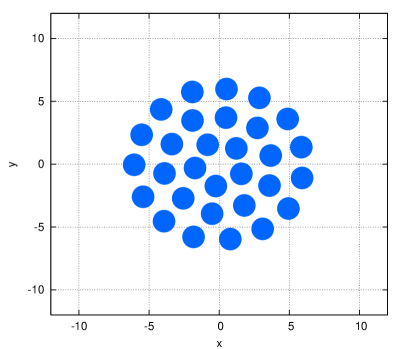
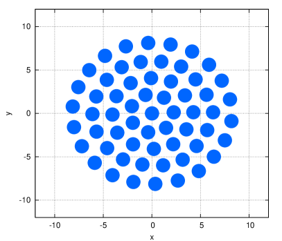
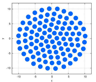
Figure 3: (color online) Stationary points for the 10, 30, 60 and 100-particle wave function at ${\lambda}=8$ with each dot’s radius set equal to $\sqrt{\tau}$.

VI Fermion Ground State PIMC

As we have shown in the last section, the determinant wave function (22) allows one to obtain excellent variational energies for up to 100 fermions (or spin-polarized electrons) in a 2D quantum dot. To lower the energy further, one can do a Fermion Ground State Path Integral Monte Carlo (FGSPIMC) calculation based on that trial function via

$$E_{0}=\lim_{\tau\rightarrow\infty}\frac{\int d{\bf X}^{\prime}d{\bf X}_{1}d{\bf X}\Psi_{D}({\bf X}^{\prime})G({\bf X}^{\prime},{\bf X}_{1};\tau)HG({\bf X}_{1},{\bf X};\tau)\Psi_{D}({\bf X})}{\int d{\bf X}^{\prime}d{\bf X}_{1}d{\bf X}\Psi_{D}({\bf X}^{\prime})G({\bf X}^{\prime},{\bf X}_{1};\tau)G({\bf X}_{1},{\bf X};\tau)\Psi_{D}({\bf X})},$$ (27)

where $G({\bf X}^{\prime},{\bf X};\tau)$ can be either the commonly used second-order primitive propagator

$$G_{2}({\bf X}^{\prime},{\bf X};\tau)={\rm e}^{-\frac{\tau}{2}V({\bf X}^{\prime})}\det\Bigl{|}\exp[-\frac{1}{2\tau}({\bf x}^{\prime}_{i}-{\bf x}_{j})^{2}]\Bigr{|}{\rm e}^{-\frac{\tau}{2}V({\bf X})},$$

or the fourth-order propagator corresponding to B2 of Ref.chin15, . To preserve the upper bound property of the Hamiltonian estimator, it is necessary to evaluate $H$ only at the middle of the integral. With anti-symmetric propagators, evaluating $H$ at any other position destroys this upper bound property. This greatly limited the choice of $G({\bf X}^{\prime},{\bf X};\tau)$. If $G_{2}({\bf X}^{\prime},{\bf X};\tau)$ is used, then (27) is a four-bead calculation, having essentially four anti-symmetric free-propagators. If the fourth-order propagator $G_{4}({\bf X}^{\prime},{\bf X};\tau)$ is used, each requiring two anti-symmetric free-propagators, then (27) is a six-bead calculation. Both will then have sign problems, with the latter more servere. However, this GSPIMC calcuation will still be better than doing a straightforward PIMC calculation. This is because for a PIMC calculation, the ground state energy can only be extract at a relatively large imaginary time, such as $\tau\approx 8$, whereas evolving from $\Psi_{D}({\bf X})$, one only needs $\tau\approx 3$ or less. This then greatly reduces the sign problem for determining the ground state energy of a large quantum dot.

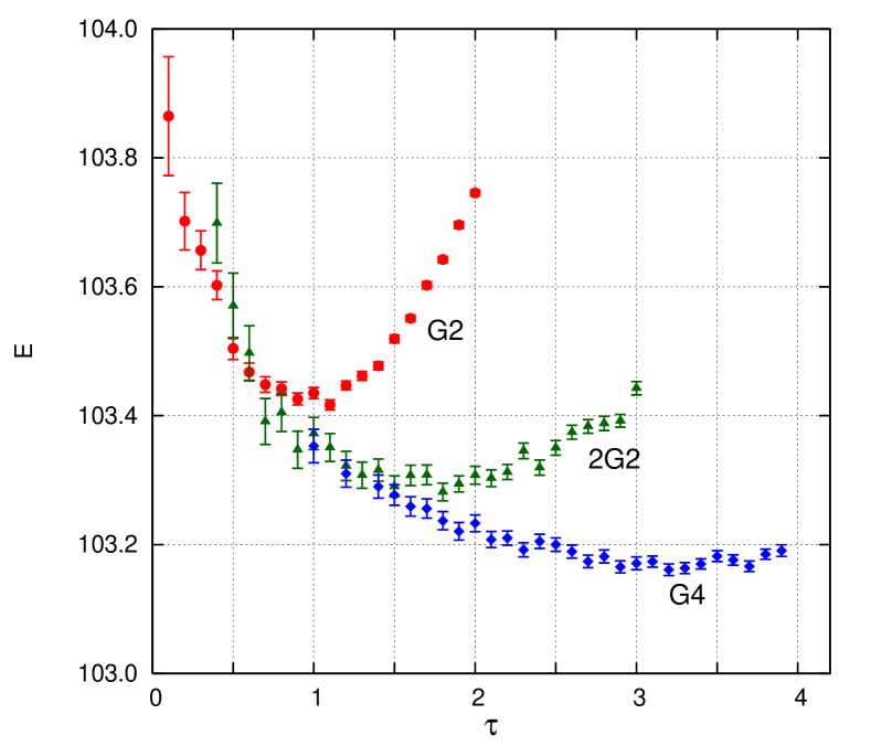
Figure 4: (color online) Ground state PIMC calculations for 8 spin-polarized electrons in a 2D harmonic oscillator at coupling ${\lambda}=8$ via (27). $G_{2}$ and $G_{4}$ are second and fourth-order imaginary time propagators respectively.

In Fig.4, we show various GSPIMC calculations for the ground state energy of 8 spin-polarized electrons at ${\lambda}=8$. Since $G_{4}$ uses two free-fermion propagators, we also computed the case with $2G2(\tau)=G_{2}(\tau/2)G_{2}(\tau/2)$, which is two second-order propagators at half the time step. The dramatic improvement in using $G_{4}$ is clearly visible. The flatness of the energy curve at large $\tau$ argues strongly that its energy is close to being exact. This is indeed the case, as shown in Table 1, where the single $G_{2}$ and $G_{4}$ energies are shown under columns GSPI2 and GSPI4 respectively. While $G_{4}$ clearly refines the energy toward the exact, its improvement over that of $G_{2}$ is a mere $\approx 0.2\%$ in the case of $N$=8. By comparison, $G_{2}$ lowers the SBWF energy by $\approx 0.8\%$. Since $G_{4}$ is a six-bead calculation, due to the sign problem, it can only be used up to $N\approx 30$. $G_{2}$ remains effective for quantum dots twice as large, up to $N\approx 60$.

While the use of GSPIMC for solving bosonic systems is fairly common, its application to fermions, due to the sign problem, has not been as prevalent. Ref.cal14, considered various choices for the free propagator, but if one views (27) as an extension of fermion PIMC, then the natural choice is to use of the anti-symmetric determinant propagator.

VII Conclusions and future directions

In this work, we have shown that 1) similarity-transformed propagators, in the case of quantum dots, can naturally produce spontaneous symmetry-breaking (SSB) wave functions for solving many-fermion problems. This is a theoretical advance in that such a SSB wave function was previously regarded only as an ad hoc ansatz. 2) Our derivation show that the particle positions of such a SSB wave function should be determined by maximizing the many-body bosonic wave function, rather than just minimizing the potential energy. 3) The use of such SSB wave function in solving the many-fermion problem via VMC is far simpler than using a determinant of excited states plus Jastrow correlators. 4) We have further demonstrated the usefulness of using higher order propagators in the context of doing fermion GSPIMC.

A natural generalization of this work is to solve for case of spin-balanced quantum dotsilk17 , with equal number of spin-up and spin-down electrons. However, the resulting SSB wave function now works less well due to spin-frustration. Take the example of $N=6$ with $N_{\uparrow}=3$ and $N_{\downarrow}=3$. In each case of $N_{\uparrow}=3$ or $N_{\downarrow}=3$, the preferred configuration is an equilateral triangle. Therefore, for $N=6$, the minimum energy configuration should be the interlacing of two equilateral triangles, forming a hexagon, with alternating spin at each vertex. However, for $N=6$, the configuration which maximizes the bosonic wave function (or that of minimizing the potential energy) is a pentagon with a single particle at the centerbed94 . Therefore one spin-up (or down) particle must be at the center. Such a wave function then frustrates the desired spin assignment and further breaks the spin-up/spin-down symmetry of the system. Moreover, for $N_{\uparrow}=N_{\downarrow}=N/2$, there are $N!/(2(N/2)!)$ distinct ways of assigning $N/2$ up spins and all are possible SSB wave functions. At this time, there is no known rule for determining which spin state will give the lowest energy. Alternatively, one can try to restore the spin-symmetry by summing over all states of distinct spin configurations. Such a multi-determinant calculation would require an order of magnitude more effort and would be best done in a future publication.

For atomic calculations, since the Hatree-Fock method generally works well and gives no indication of any SSB state, the method proposed here will probably not be applicable. However, for nuclei calculations, since our method is exact for non-interacting fermions in a harmonic oscillator (which is the basis of the shell-model), our method may be useful for calculating alpha-particle clustered nuclei such as $C^{12},O^{16},N\!e^{20},$ etc., since alpha-particle clustering can be viewed as a SSB state.

- (1) S. M. Reimann and M. Manninen, Rev. Mod. Phys. 74, 1283 (2002).
- (2) S. M. Blinder, J. Math. Phys. 36, 1208 (1995)
- (3) N. R. Kestner and O. Sinanoglu, Phys. Rev. 128, 2687 (1962)
- (4) C. Yannouleas and U. Landman Phys. Rev. Lett. 82, 5325 (1999)– Erratum Phys. Rev. Lett. 85, 2220 (2000)
- (5) M. Ferconi and G. Vignale Phys. Rev. B 50, 14722 (1999)
- (6) K. Hirose and N. S. Wingreen Phys. Rev. B 59, 4604 (1999).
- (7) M. Rontani, C. Cavazzoni, D. Bellucci and G. Goldoni J. Chem. Phys. 124, 124102 (2006).
- (8) E. Waltersson, C. J. Wesslen, and E. Lindroth, Phys. Rev. B 87, 035112 (2011).
- (9) M. Pedersen Lohne, G. Hagen, M. Hjorth-Jensen, S. Kvaal, and F. Pederiva, Phys. Rev. B 84, 115302 (2011).
- (10) A. Harju, S. Siljamaki, and R. M. Nieminen Phys. Rev. B 65, 075309 (2002)
- (11) J. Kainz, S. A. Mikhailov, A. Wensauer, and U. Rössler, Phys. Rev. B 65, 115305 (2002).
- (12) F. Pederiva, C.J. Umrigar and E. Lipparini, Phys. Rev. B 62, 8120 (2000), B 68, 089901(E) (2003)
- (13) A. Ghosal, A. D. Güclü, C. J. Umrigar, D. Ullmo and H. U. Baranger Phys. Rev. B 76, 085341 (2007)
- (14) C. H. Mak, R. Egger, and H. Weber-Gottschick, Phys. Rev. Lett. 81, 4533 (1998).
- (15) R. Egger, W. Häusler, C. H. Mak and H. Grabert, Phys. Rev. Lett. 82, 3320 (1999); 83, 462(E) (1999).
- (16) R. Egger, L. Mühlbacher, and C. H. Mak, Phys. Rev. E 61, 5961 (2000).
- (17) B. Reusch and R. Egger, Europhys. Lett. 64, 84 (2003).
- (18) Siu A. Chin, Phys. Rev. E 91, 031301(R) (2015).
- (19) Ilkka Kylanpaa and Esa Rasanen Phys. Rev. B 96, 205445 (2017)
- (20) D. M. Ceperley, Rev. Mod. Phys., 67, 279 (1995).
- (21) A. Sarsa, K. E. Schmidt, and W. R. Magro, J. Chem. Phys. 113, 1366 (2000).
- (22) F. Calcavecchia, F. Pederiva, M. H. Kalos, and Thomas D. Kühne, Phys. Rev. E 90, 053304 (2014)
- (23) S. A. Mikhailov, Physica B 299, 6 (2001).
- (24) C. Yannouleas and U. Landman, Phys. Rev. B 66, 115315 (2002).
- (25) C. Yannouleas and U. Landman, Rep. Prog. Phys. 70 (2007) 2067–2148.
- (26) Siu A. Chin, “Quadratic diffusion Monte Carlo algorithms for solving atomic many-body problems”, Phys. Rev. A 42, 6991 (1990).
- (27) J. W. Moskowitz, K. E. Schmidt, M. E. Lee, and M. H. Kalos, J. Chem. Phys. 77, 349 (1982).
- (28) P. J. Reynolds, D. M. Ceperley, B. J. Adler, and W. A. Lester, J. Chem. Phys. 77, 5593 (1982).
- (29) M. Caffarel and P. Claverie, J. Chem. Phys. 88, 1088 (1988); 88, 1100 (1988).
- (30) G. E. Uhlenbeck and L. S. Ornstein, Phys. Rev. 36, 823–841 (1930)
- (31) N. Metropolis, A. W. Rosenbluth, M. N. Rosenbluth, A. H. Teller and E. Teller, J. Chem. Phys. 21, 1087 (1953)
- (32) V. M. Bedanov and F. M. Peeters Phys. Rev. B 49, 2667–2675 (1994)