A Near-Optimal Change-Detection Based Algorithm for Piecewise-Stationary Combinatorial Semi-Bandits

Abstract

We investigate the piecewise-stationary combinatorial semi-bandit problem. Compared to the original combinatorial semi-bandit problem, our setting assumes the reward distributions of base arms may change in a piecewise-stationary manner at unknown time steps. We propose an algorithm, GLR-CUCB, which incorporates an efficient combinatorial semi-bandit algorithm, CUCB, with an almost parameter-free change-point detector, the Generalized Likelihood Ratio Test (GLRT). Our analysis shows that the regret of GLR-CUCB is upper bounded by $\mathcal{O}(\sqrt{NKT\log{T}})$, where $N$ is the number of piecewise-stationary segments, $K$ is the number of base arms, and $T$ is the number of time steps. As a complement, we also derive a nearly matching regret lower bound on the order of $\Omega(\sqrt{NKT}$), for both piecewise-stationary multi-armed bandits and combinatorial semi-bandits, using information-theoretic techniques and judiciously constructed piecewise-stationary bandit instances. Our lower bound is tighter than the best available regret lower bound, which is $\Omega(\sqrt{T})$. Numerical experiments on both synthetic and real-world datasets demonstrate the superiority of GLR-CUCB compared to other state-of-the-art algorithms.

1 Introduction

The multi-armed bandit (MAB) problem, first proposed by Thompson (1933), has been studied extensively in statistics and machine learning communities, as it models many online decision making problems such as online recommendation (Li et al., 2016), computational advertising (Tang et al., 2013), and crowdsourcing task allocation (Hassan and Curry, 2014). The classical MAB is modeled as an agent repeatedly pulling one of $K$ arms and observing the reward generated, with the goal of minimizing the regret which is the difference between the reward of the optimal arm in hindsight and the reward of the arm chosen by the agent. This classical problem is well understood for both stochastic (Lai and Robbins, 1985) and adversarial settings (Auer et al., 2002b). The stochastic setting is when the reward of each arm is generated from a fixed distribution, and it is well known that the problem-dependent lower bound is of order $\Omega(\log T)$ (Lai and Robbins, 1985), where $T$ is the number of time steps. Several algorithms have been proposed and proven to achieve $\mathcal{O}(\log T)$ regret (Agrawal and Goyal, 2012; Auer et al., 2002a). The adversarial setting is when at each time step the environment generates the reward in an adversarial manner, whose minimax regret lower bound is of order $\Omega(\sqrt{T})$. Several algorithms achieving order-optimal (up to poly-logarithm factors) regret have been proposed in recent years (Hazan and Kale, 2011; Bubeck et al., 2018; Li et al., 2019).

Many real-world applications, however, have a combinatorial nature that cannot be fully characterized by the classical MAB model. For example, online movie sites aim to recommend multiple movies to the users to maximize their utility under some constraints (e.g. recommend at most one movie for each category). This phenomenon motivates the study of combinatorial semi-bandits (CMAB), which aims to identify the best superarm, a set of base arms with highest aggregated reward. Several algorithms for stochastic CMAB with provable guarantees based on optimism principle have been proposed recently (Chen et al., 2013; Kveton et al., 2015; Combes et al., 2015). All of these algorithms use some oracle to overcome the curse of dimension of the action space for solving some combinatorial optimization problem at each iteration. In addition, these algorithms achieve the optimal regret upper bound which is $\mathcal{O}(C\log T)$, where $C$ is an instance-dependent parameter. Adversarial CMAB is also well studied. Several algorithms achieve optimal regret of order $\mathcal{O}(\sqrt{T})$ based on either Follow-the-Regularized-Leader or Follow-the-Perturbed-Leader, both of which are general frameworks for adversarial online learning algorithm design (Hazan, 2016). Moreover, one recent study has developed an algorithm that is order-optimal for both stochastic and adversarial CMAB (Zimmert et al., 2019).

Although both stochastic and adversarial CMAB are well-studied, understanding of the scenario lying in the “middle” of these two settings is still limited. Such a “middle” setting where the reward distributions of base arms slowly change over time may be a more realistic model in many applications. For instance, in online recommendation systems, users’ preference are unlikely to be either time-invariant or to change significantly and frequently over time. Thus in this case it would be too ideal to assume the stochastic CMAB model and too conservative to assume the adversarial CMAB model. Similar situations appear in web search, online advertisement, and crowdsourcing (Yu and Mannor, 2009; Pereira et al., 2018; Vempaty et al., 2014). As such, we investigate a setting lying between these two standard CMAB models, namely piecewise-stationary combinatorial semi-bandit, which we will define formally in Section 2. Piecewise-stationary CMAB is a natural generalization of the piecewise-stationary MAB model (Hartland et al., 2007; Kocsis and Szepesvári, 2006; Garivier and Moulines, 2011), and can be interpreted as an approximation to the slow-varying CMAB problem. Roughly, compared to the stochastic CMAB, we assume reward distributions of base arms remain fixed for certain time periods called piecewise-stationary segments, but can change abruptly at some unknown time steps, called change-points.

Previous works on piecewise-stationary MAB may be divided into two categories: passively adaptive approach (Garivier and Moulines, 2011; Besbes et al., 2014; Wei and Srivatsva, 2018) and actively adaptive approach (Cao et al., 2019; Liu et al., 2018; Besson and Kaufmann, 2019; Auer et al., 2019). Passively adaptive approaches make decisions based on the most recent observations and are unaware of the underlying distribution changes. On the contrary, actively adaptive approaches incorporate a change-point detector subroutine to monitor the reward distributions, and restart the algorithm once a change-point is detected. Numerous empirical experiments have shown that actively adaptive approaches outperform passively adaptive approaches (Mellor and Shapiro, 2013), which motivates us to adopt an actively adaptive approach.

Our main contributions include the following:

• We propose a simple and general algorithm for piecewise-stationary CMAB, named GLR-CUCB, which is based on CUCB (Chen et al., 2013) with a novel change-point detector, the generalized likelihood ratio test (GLRT)  (Besson and Kaufmann, 2019). The advantage of GLRT change-point detection is it is almost parameter-free and thus easy to tune compared to previously proposed change-point detection methods used in nonstationary MAB, such as CUSUM (Liu et al., 2018) and SW (Cao et al., 2019).

• For any combinatorial action set, we derive the problem-dependent regret bound for GLR-CUCB under mild conditions (see Section 4). When the number of change points $N$ is known beforehand, the regret of GLR-CUCB is upper bounded by $\mathcal{O}(C_{1}NK^{2}\log{T}+C_{2}\sqrt{NKT\log{T}})$ (nearly order-optimal within poly-logarithm factor in $T$), where $K$ is number of base arms. When $N$ is unknown, the algorithm achieves $\mathcal{O}(C_{1}NK^{2}\log{T}+C_{2}N\sqrt{KT\log{T}})$. Here, $C_{1}$ and $C_{2}$ are problem-dependent constants which do not depend on $T$, $N$, or $K$.

• We derive a tighter minimax lower bound for both piecewise-stationary MAB and piecewise-stationary CMAB on the order of $\Omega(\sqrt{NKT})$. Since piecewise-stationary MAB is a special instance of piecewise-stationary CMAB in which every superarm is a single arm, thus any minimax lower bound holds for piecewise-stationary MAB also holds for piecewise-stationary CMAB. To the best of our knowledge, this is the best existing minimax lower bound for piecewise-stationary CMAB. Previously, the best available lower bound is $\Omega(\sqrt{T})$ (Garivier and Moulines, 2011), which does not depend on $N$ or $K$.

• We demonstrate that GLR-CUCB performs significantly better than state-of-the-art algorithms through experiments on both synthetic and real-world datasets.

The remainder of this paper is organized as follows: the formal problem formulation and some preliminaries are introduced in Section 2, then the proposed GLR-CUCB algorithm in Section 3. We derive the upper bound on the regret of our algorithm in Section 4, and the minimax regret lower bound in Section 5. Section 6 gives our experiment results. Finally, we conclude the paper. Due to the page limitation, we postpone proofs and additional experimental results to the appendix.

2 Problem Formulation and Background

In this section, we start with the formal definition of piecewise-stationary combinatorial semi-bandit as well as some technical assumptions in Section 2.1. Then, we introduce the GLR change-point detector used in our algorithm design, and its advantage in Section 2.2.

2.1 Piecewise-Stationary Combinatorial Semi-Bandits

A piecewise-stationary combinatorial semi-bandit is characterized by a tuple $(\mathcal{K},\mathcal{F},\mathcal{T},\{f_{k,t}\}_{k\in\mathcal{K},t\in\mathcal{T}},r_{\bm{\mu}_{t}}\left(S_{t}\right))$. Here, $\mathcal{K}=\{1,\ldots,K\}$ is the set of $K$ base arms; $\mathcal{F}\subseteq 2^{\mathcal{K}}$ is the set of all super arms; $\mathcal{T}=\{1,\ldots,T\}$ is a sequence of $T$ time steps; $f_{k,t}$ is the reward distribution of arm $k$ at time $t$ with mean $\mu_{k,t}$ and bounded support within $[0,1]$; $r_{\bm{\mu}_{t}}\left(S_{t}\right):\mathcal{F}\times[0,1]^{K}\mapsto\mathbb{R}$ is the expected reward function defined on the super arm $S_{t}$ and mean vector of all base arms $\bm{\mu}_{t}:=[\mu_{1,t},\mu_{2,t},\ldots,\mu_{K,t}]^{\top}$ at time $t$. Like Chen et al. (2013), we assume the expected reward function $r_{\bm{\mu}}\left(S\right)$ satisfies the following two properties:

Assumption 2.1 (Monotonicity).

Given two arbitrary mean vectors $\bm{\mu}$ and $\bm{\mu}^{\prime}$, if $\mu_{k}\geq\mu^{\prime}_{k},\ \forall k\in\mathcal{K}$, then $r_{\bm{\mu}}\left(S\right)\geq r_{\bm{\mu}^{\prime}}\left(S\right)$.

Assumption 2.2 ($L$-Lipschitz).

Given two arbitrary mean vectors $\bm{\mu}$ and $\bm{\mu}^{\prime}$, there exists an $L<\infty$ such that $\left|r_{\bm{\mu}}\left(S\right)-r_{\bm{\mu}^{\prime}}\left(S\right)\right|\leq L\|\mathcal{P}_{S}(\bm{\mu}-\bm{\mu}^{\prime})\|_{2}$, $\forall S\in\mathcal{F}$, where $\mathcal{P}_{S}(\cdot)$ is the projection operator specified as $\mathcal{P}_{S}(\bm{\mu})=\left[\mu_{1}\mathbb{I}\{1\in S\},\ldots,\mu_{k}\mathbb{I}\{k\in S\},\ldots,\mu_{K}\mathbb{I}\{K\in S\}\right]^{\top}$ in terms of the indicator function $\mathbb{I}\{\cdot\}$.

In the piecewise i.i.d. model, we define $N$, the number of piecewise-stationary segments in the reward process, to be

$$N=1+\sum_{t=1}^{T-1}\mathbb{I}{\{\exists k\in\mathcal{K}~{}\mbox{s.t.}~{}f_{k,t}\neq f_{k,t+1}\}}.$$

We denote these $N-1$ change-points as $\nu_{1},\nu_{2},\ldots,\nu_{N-1}$ respectively, and we let $\nu_{0}=0$ and $\nu_{N}=T$. For each piecewise-stationary segment $t\in[\nu_{i-1}+1,\nu_{i}]$, we use $f_{k}^{i}$ and $\mu_{k}^{i}$ to denote the reward distribution and the expected reward of arm $k$ on the $i$th piecewise-stationary segment, respectively. The vector encoding the expected rewards of all base arms at the $i$th segment is denoted as $\bm{\mu}^{i}=[\mu_{1}^{i},\cdots,\mu_{K}^{i}]^{\top}$, $\forall i=1,\cdots,N$. Note that when a change-point occurs, there must be at least one arm whose reward distribution has changed, however, the rewards distributions of all base arms do not necessarily change.

For a piecewice-stationary combinatorial semi-bandit problem, at each time step $t$, the learning agent chooses a super arm $S_{t}\in\mathcal{F}$ to play based on the rewards observed up to time $t$. When the agent plays a super arm $S_{t}$, the reward $\{X_{I_{t}}\}_{I_{t}\in S_{t}}$ of base arms contained in super arm $S_{t}$ are revealed to the agent and the reward of super arm $R_{t}(S_{t})$ as well. We assume that the agent has access to an $\alpha$-approximation oracle, to carry out combinatorial optimization, defined as follows.

Assumption 2.3 ($\alpha$-approximation oracle).

Given a mean vector $\bm{\mu}$, the $\alpha$-approximation oracle $\mbox{Oracle}_{\alpha}(\bm{\mu})$ outputs an $\alpha$-suboptimal super arm $S$ such that $r_{\bm{\mu}}\left(S\right)\geq\alpha\max_{S\in\mathcal{F}}r_{\bm{\mu}}\left(S\right)$.

Remark 2.1.

The approximation oracle assumption was first proposed in Chen et al. (2013) for the combinatorial semi-bandit setting. This assumption is reasonable since many combinatorial NP-hard problems admit approximation algorithms, which can be solved efficiently in polynomial time (Ausiello et al., 1995). There are also many combinatorial problems which are not NP hard and can be solved efficiently. One example is the top-$m$ arm identification problem in the bandit setting (Cao et al., 2015), where any efficient sorting algorithm suffices.

As only an $\alpha$-approximation oracle is used for optimization, it is reasonable to use expected $\alpha$-approximation cumulative regret to measure the performance of the learning agent, defined as follows.

Definition 2.4 (Expected $\alpha$-approximation cumulative regret).

The agent’s policy is evaluated by its expected $\alpha$-approximation cumulative regret,

$$\mathcal{R}(T)=\mathbb{E}\left[\alpha\sum_{t=1}^{T}\max_{S\in\mathcal{F}}r_{\bm{\mu}_{t}}(S)-\sum_{t=1}^{T}r_{\bm{\mu}_{t}}(S_{t})\right],$$

where the expectation $\mathbb{E}[\cdot]$ is taken with respect to the selection of $\{S_{t}|S_{t}\in\mathcal{F}\}$.

2.2 Generalized Likelihood Ratio Change-Point Detector for Sub-Bernoulli Distribution

Sequential change-point detection is a classical problem in statistical sequential analysis, but most existing works make additional assumptions on the pre-change and post-change distributions which might not hold in the bandit setting (Siegmund, 2013; Basseville and Nikiforov, 1993). In general, designing algorithms with provable guarantees for change detection with little assumption on pre-change and post-change distributions is very challenging. In our algorithm design, we will use the generalized likelihood ratio (GLR) change-point detector (Besson and Kaufmann, 2019), which works for any sub-Bernoulli distribution. Compared to other existing change detection methods used in piecewise-stationary MAB, the GLR detector has less parameters to be tuned and needs less prior knowledge for the bandit instance. Specifically, GLR only needs to tune the threshold $\delta$ for the change-point detection, and does not require the smallest change in expectation among all change-points. On the contrary, CUSUM (Liu et al., 2018) and SW (Cao et al., 2019) both need more parameters to be tuned and need to know the smallest magnitude among all change-points beforehand, which limits their practicality.

To define GLR change-point detector, we need some more definitions for clarity. A distribution $f$ is said to be sub-Bernoulli if $\mathbb{E}_{X\sim f}[e^{\lambda X}]\leq e^{\phi_{\mu}(\lambda)}$, where $\mu=\mathbb{E}_{X\sim f}[X]$; $\phi_{\mu}(\lambda)=\log(1-\mu-\mu e^{\lambda})$ is the log moment generating function of a Bernoulli distribution with mean $\mu$. Notice that the support of reward distribution $f_{k,t}$, $\forall k\in\mathcal{K},\,t\in\mathcal{T}$ is a subset of the interval $[0,1]$, thus all $\{f_{k,t}\}$ are sub-Bernoulli distributions with mean $\{\mu_{k,t}\}$, due to the following lemma.

Lemma 2.5 (Lemma 1 in Cappé et al. (2013)).

Any distribution $f$ with bounded support within the interval $[0,1]$ is a sub-Bernoulli distribution that satisfies:

$$\mathbb{E}_{X\sim f}[e^{\lambda X}]\leq e^{\phi_{\mu}(\lambda)}.$$

Suppose we have either a time sequence $\{X_{t}\}_{t=1}^{n}$ drawn from a sub-Bernoulli distribution for any $t\leq n$ or two sub-Bernoulli distributions with an unknown change-point $s\in[1,n-1]$. This problem can be formulated as a parametric sequential test:

$$\mathcal{H}_{0} :\exists f_{0}:X_{1},\ldots,X_{n}\overset{i.i.d.}{\sim}~{}f_{0},$$

$$\mathcal{H}_{1} :\exists f_{0}\neq f_{1},\,\tau\in[1,n-1]:\,X_{1},\ldots,X_{\tau}\overset{i.i.d.}{\sim}f_{0}~{}\mbox{and}~{}X_{\tau+1},\ldots,X_{n}\overset{i.i.d.}{\sim}f_{1}.$$

The GLR statistic for sub-Bernoulli distributions is:

$$\text{GLR}(n)=\sup_{s\in[1,n-1]}\quad[s\times\text{kl}(\hat{\mu}_{1:s},\hat{\mu}_{1:n})+(n-s)\times\text{kl}\left(\hat{\mu}_{s+1:n},\hat{\mu}_{1:n}\right)],$$ (1)

where $\hat{\mu}_{s:s^{\prime}}$ is the mean of the observations collected between $s$ and $s^{\prime}$, and $\mbox{kl}(x,y)$ is the binary relative entropy between Bernoulli distributions,

$$\mbox{kl}(x,y)=x\log\left(\frac{x}{y}\right)+(1-x)\log\left(\frac{1-x}{1-y}\right).$$

If the GLR in Eq. (1) is large, it indicates that hypothesis $\mathcal{H}_{1}$ is more likely. Now, we are ready to define the sub-Bernoulli GLR change-point detector with confidence level $\delta\in(0,1)$.

Definition 2.6.

The sub-Bernoulli GLR change-point detector with threshold function $\beta(n,\delta)$ is

$$\tau:=\inf\{n\in\mathbb{N}:\sup_{s\in[1,n-1]}\quad[s\times\mbox{kl}(\hat{\mu}_{1:s},\hat{\mu}_{1:n})+(n-s)\times\mbox{kl}(\hat{\mu}_{s+1:n},\hat{\mu}_{1:n})]\geq\beta(n,\delta)\},$$

where $\beta(n,\delta)=2\mathcal{Q}\left(\frac{\log(3n\sqrt{n}/\delta)}{2}\right)+6\log(1+\log(n))$, and $\mathcal{Q}(\cdot)$ is as in Eq. (13) in Kaufmann and Koolen (2018).

The pseudo-code of sub-Bernoulli GLR change-point detector is summarized in Algorithm 1 for completeness.

Algorithm 1 Sub-Bernoulli GLR Change-Point Detector: $\mbox{GLR}(X_{1},\cdots,X_{n};\delta)$

0:  observations $X_{1},\ldots,X_{n}$ and confidence level $\delta$.

1:  if $\sup_{s\in[1,n-1]}\quad[s\times\mbox{kl}(\hat{\mu}_{1:s},\hat{\mu}_{1:n})+(n-s)\times\mbox{kl}(\hat{\mu}_{s+1:n},\hat{\mu}_{1:n})]\geq\beta(n,\delta)$ then

2:     Return True

3:  else

4:     Return False

5:  end if

3 The GLR-CUCB Algorithm

Our proposed algorithm, GLR-CUCB, incorporates an efficient combinatorial semi-bandit problem algorithm CUCB (Chen et al., 2013) with a change-point detector running on each base arm (See Algorithm 2). The GLR-CUCB requires the number of time steps $T$, the number of base arms $K$, uniform exploration probability $p$, and the confidence level $\delta$ as inputs. Let $\tau$ denote the last change-point detection time, and $n_{k}$ denote the number of observations of base arm $k$ after $\tau$, which are initialized as zeros at the beginning of the algorithm.

At each time step, the GLR-CUCB first determines if it will enter forced uniform exploration (to ensure each base arm collects sufficient samples for the change-point detection) according to the condition in line 3. If it is in a forced exploration, a random super arm $S_{t}$ that contains $a$ (line 4) is played, to ensure sufficient number of samples are collected for every base arm. Otherwise, the next super arm $S_{t}$ to be played is determined by the $\alpha$-approximation oracle $\mbox{Oracle}_{\alpha}(\cdot)$ (line 6) given the UCB indices (line 19). Then, the learning agent plays the super arm $S_{t}$, and gets the reward $R_{t}\left(S_{t}\right)$ of the super arm $S_{t}$ and the rewards $\{X_{I_{t}}\}_{I_{t}\in S_{t}}$ of the base arm $I_{t}$’s that are contained in the super arm $S_{t}$ (line 8). In the next step, the algorithm updates the statistics for each base arm (lines 10-11) in order to run the GLR change-point detector (Algorithm 1) with confidence level $\delta$ (line 12). If the GLR change-point detector detects a change in distribution for any of the base arms, the algorithm sets $\tau$ to be the current time step and all $n_{k}$’s to be 0 (line 13-14) before going into time step $t+1$. Lastly, the UCB indices of all base arms are updated (line 19).

Algorithm 2 The GLR-CUCB Algorithm

0:  $T\in\mathbb{N}$, $K\in\mathbb{N}$, exploration probability $p\in(0,1)$, confidence level $\delta\in(0,1)$.

1:  Initialization: $\forall k\in\mathcal{K}$, $n_{k}\leftarrow 0$; $\tau\leftarrow 0$.

2:  for all $t=1,2,\ldots,T$ do

3:     if $p>0$ and $a\leftarrow(t-\tau)\mod\left\lfloor\frac{K}{p}\right\rfloor\in\mathcal{K}$ then

4:        Randomly choose $S_{t}$ with $a\in S_{t}$.

5:     else

6:        $S_{t}=\mbox{Oracle}_{\alpha}\left(\mbox{UCB}\right)$.

7:     end if

8:     Play super arm $S_{t}$ and get the reward $R_{t}(S_{t})$ and $X_{I_{t},t},\,\forall I_{t}\in S_{t}$.

9:     for all $I_{t}\in S_{t}$ do

10:        $Z_{I_{t},n_{I_{t}}}\leftarrow X_{I_{t},t}$.

11:        $n_{I_{t}}\leftarrow n_{I_{t}}+1$.

12:        if $\mbox{GLR}\left(Z_{I_{t},1},\cdots,Z_{I_{t},n_{I_{t}}};\delta\right)=\text{True}$ then

13:           $n_{k}\leftarrow 0,\forall k\in\mathcal{K}$.

14:           $\tau\leftarrow t$.

15:        end if

16:     end for

17:     for all $k=1,\cdots,K$ do

18:        if $n_{k}\neq 0$ then

19:           $\text{UCB}(k)\leftarrow\frac{1}{n_{\ell}}\sum_{n=1}^{n_{k}}Z_{k,n}+\sqrt{\frac{3\log(t-\tau)}{2n_{k}}}$.

20:        end if

21:     end for

22:  end for

Remark 3.1.

The uniform exploration is necessary for this algorithm, and similar strategy has been adopted in Liu et al. (2018); Cao et al. (2019). Intuitively, uniform exploration ensures each base arm gathers sufficient samples to guarantee quick change detection whereas pure UCB exploration is incapable of this. One more rigorous argument is given in Garivier and Moulines (2011), which shows that theoretically pure UCB exploration performs badly on piecewise-stationary MAB.

Remark 3.2.

Thompson sampling (TS) often performs better than UCB policy in empirical simulations, but it has been shown that one cannot incorporate an approximate oracle in TS for even MAB problems (Wang and Chen, 2018). Thus our algorithm adopts UCB policy for the bandit component to ensure compatibility with approximation oracle.

4 Regret Upper Bound

In this section, we analyze the $T$-step regret of our proposed algorithm GLR-CUCB. Recall $T$ is the time horizon, $N$ is the number of piecewise-stationary segments, $\nu_{1},\ldots,\nu_{N-1}$ are the change-points, and for each segment $i\in[N]$, $\bm{\mu}^{i}\in\mathbb{R}^{K}$ is the vector encoding the expected rewards of all base arms. A super arm $S$ is bad with respect to the $i$th piecewise-stationary distributions if $r_{\bm{\mu}^{i}}(S)\leq\alpha\max_{\tilde{S}\in\mathcal{F}}r_{\bm{\mu}^{i}}(\tilde{S})$. We define $\mathcal{S}_{B}^{i}=\{S|r_{\bm{\mu}^{i}}(S)\leq\alpha\max_{\tilde{S}\in\mathcal{F}}r_{\bm{\mu}^{i}}(\tilde{S})\}$ to be the set of bad super arms with respect to the $i$th piecewise-stationary segment. We define the suboptimality gap in the $i$th stationary segment as follows:

$$\Delta^{\text{min},i}_{\textup{opt}} =\alpha\max_{\tilde{S}\in\mathcal{F}}r_{\bm{\mu}^{i}}(\tilde{S})-\max\{r_{\bm{\mu}^{i}}(S)|S\in\mathcal{S}_{B}^{i}\},$$

$$\Delta^{\text{max},i}_{\textup{opt}} =\alpha\max_{\tilde{S}\in\mathcal{F}}r_{\bm{\mu}^{i}}(\tilde{S})-\min\{r_{\bm{\mu}^{i}}(S)|S\in\mathcal{S}_{B}^{i}\}.$$

Furthermore, let $\Delta^{\text{max}}_{\textup{opt}}=\max_{i\in[N]}\Delta^{\text{max},i}_{\textup{opt}}$ and $\Delta^{\text{min}}_{\textup{opt}}=\min_{i\in[N]}\Delta^{\text{min},i}_{\textup{opt}}$ be the maximum and minimum sub-optimal gaps for the whole time horizon, respectively. Lastly, denote the largest gap at change-point $\nu_{i}$ as $\Delta_{\textup{change}}^{i}=\max_{k\in\mathcal{K}}\left|\mu_{k}^{i+1}-\mu_{k}^{i}\right|$, $\forall 1\leq i\leq N-1$, and $\Delta^{0}_{\textup{change}}=\max_{k\in\mathcal{K}}\left|\mu_{k}^{1}\right|$. We need the following assumption for our theoretical analysis.

Assumption 4.1.

Define $d_{i}=d_{i}(p,\delta)=\left\lceil\{4K/p\left(\Delta_{\textup{change}}^{i}\right)^{2}\}\beta(T,\delta)+\frac{K}{p}\right\rceil$ and assume $\nu_{i}-\nu_{i-1}\geq 2\max\{d_{i},d_{i-1}\}$, $\forall i=1,\ldots,N-1$, where $\nu_{N}-\nu_{N-1}\geq 2d_{N-1}$.

Tuning $\delta$ and $p$ properly (See Corollary 4.3), and applying the upper bound on $\mathcal{Q}(x)$ by Kaufmann and Koolen (2018) with $x\geq 5$,

$$\mathcal{Q}(x)\leq x+4\log(1+x+\sqrt{2x}),$$

the length of each piecewise-stationary segment is $\Omega(\sqrt{T\log{T}})$. Roughly, we assume the length of each stationary segment to be sufficiently long, in order to let the GLR change-point detector detect the change in distribution within a reasonable delay with high probability. Similar assumption on the length of stationary segments also appears in other literature on piecewise stationary MAB (Liu et al., 2018; Cao et al., 2019; Besson and Kaufmann, 2019). Note that Assumption 4.1 is only required for the theoretical analysis; Algorithm 2 can be implemented regardless of this assumption. Now we are ready to state the regret upper bound for Algorithm 2.

Theorem 4.2.

Running GLR-CUCB with Assumptions 2.1, 2.2, and 4.1, the expected $\alpha$-approximation cumulative regret of GLR-CUCB with exploration probability $p$ and confidence level $\delta$ satisfies

$$\mathcal{R}(T)\leq\underbrace{\sum_{i=1}^{N}\widetilde{C}_{i}}_{(a)}+\underbrace{\Delta^{\text{max}}_{\textup{opt}}Tp}_{(b)}+\underbrace{\sum_{i=1}^{N-1}\Delta^{\text{max},i+1}_{\textup{opt}}d_{i}}_{(c)}+\underbrace{3NT\Delta^{\text{max}}_{\textup{opt}}K\delta}_{(d)},$$

where $\widetilde{C}_{i}=\left(6L^{2}K^{2}\log{T}/\left(\Delta^{\text{min},i}_{\textup{opt}}\right)^{2}+\pi^{2}/6+K\right)\Delta^{\text{max},i}_{\textup{opt}}$.

Theorem 4.2 indicates that the regret comes from four sources. Terms (a) and (b) correspond to the cost of exploration, while terms (c) and (d) correspond to the cost of change-point detection. More specifically, term (a) is due to UCB exploration, term (b) is due to uniform exploration, term (c) is due to expected delay of GLR change-point detector, and term (d) is due to the false alarm probability of GLR change-point detector. We need to carefully tune the exploration probability $p$ and false alarm probability $\delta$ to balance the trade-off.

The following corollary comes directly from Theorem 4.2 by properly tuning the parameters in the algorithm.

Corollary 4.3.

Let $\Delta^{\text{min}}_{\textup{change}}=\min_{i\in[N-1]}\Delta_{\textup{change}}^{i}$, we have

1. ($N$ is known) Choosing $\delta=\frac{1}{T}$, $p=\sqrt{\frac{NK\log{T}}{T}}$, gives $\mathcal{R}(T)=\mathcal{O}\left(\frac{NK^{2}\log{T}\Delta^{\text{max}}_{\textup{opt}}}{\left(\Delta^{\text{min}}_{\textup{opt}}\right)^{2}}+\frac{\sqrt{NKT\log{T}}\Delta^{\text{max}}_{\textup{opt}}}{\left(\Delta^{\text{min}}_{\textup{change}}\right)^{2}}\right)$;

2. ($N$ is unknown) Choosing $\delta=\frac{1}{T}$, $p=\sqrt{\frac{K\log{T}}{T}}$, gives $\mathcal{R}(T)=\mathcal{O}\left(\frac{NK^{2}\log{T}\Delta^{\text{max}}_{\textup{opt}}}{\left(\Delta^{\text{min}}_{\textup{opt}}\right)^{2}}+\frac{N\sqrt{KT\log{T}}\Delta^{\text{max}}_{\textup{opt}}}{\left(\Delta^{\text{min}}_{\textup{change}}\right)^{2}}\right)$.

Remark 4.1.

The effect of oracle is to reduce the dependency on number of base arms $K$ from $|\mathcal{F}|$ to $K^{2}$ during exploration (first term in the regret appeared in Corollary 4.3). In the worst case, $|\mathcal{F}|$ can be exponential with respect to $K$. Recall that if we use standard MAB algorithms for exploration, the dependency on $K$ is $|\mathcal{F}|$.

Remark 4.2.

As $T$ becomes larger, the regret is dominated by the cost of change-point detection, which has similar order compared to the regret bound of piecewise-stationary MAB algorithms. This is reasonable since our setting assumes that we have access to the reward of the base arms contained in the super arm played by the agent.

Remark 4.3.

When $T$ is large, the order of the regret bound is similar to the regret bound of adversarial bandit. But note that regret definition for adversarial bandit and piecewise-stationary bandit is different. For the first case, the regret is evaluated with respect to one fixed arm which is optimal for the whole horizon. But for the second case, the regret is evaluated with respect to point-wise optimal arm, which is much more challenging.

We can use Corollary 4.3 as a guide for parameter tuning. The above corollary indicates that without knowledge of the number of change-points $N$, we pay a penalty of a factor of $\sqrt{N}$ in the long run.

For the detailed proof of Theorem 4.2, see Appendix A. Here we sketch the proof; to do so we need some additional lemmas. We start by proving the regret of GLR-CUCB under the stationary scenario.

Lemma 4.4.

Under the stationary scenario, i.e. $N=1$, the $\alpha$-approximation cumulative regret of GLR-CUCB is upper bounded as:

$$\mathcal{R}(T)\leq\Delta^{\text{max},1}_{\textup{opt}}T\mathbb{P}(\tau_{1}\leq T)+\Delta^{\text{max},1}_{\textup{opt}}Tp+\widetilde{C}_{1}.$$

The first term is due to the possible false alarm of the change-point detection subroutine, the second term is due to the uniform exploration, and the last term is due to the UCB exploration. We upper bound the false alarm probability in Lemma 4.5, as follows.

Lemma 4.5 (False alarm probability in the stationary scenario).

Consider the stationary scenario, i.e. $N=1$, with confidence level $\delta>0$; we have that

$$\mathbb{P}\left(\tau_{1}\leq T\right)\leq K\delta.$$

Remark 4.4.

By setting $\delta=\frac{1}{T}$, we will have $\mathbb{P}\left(\tau_{1}\leq T\right)\leq\frac{K}{T}$. Asymptotically, the false alarm probability will go to 0.

In the next lemma, we show the GLR change-point detector is able to detect change in distribution reasonably well with high probability, given all previous change-points were detected reasonably well. The formal statement is as follows.

Lemma 4.6.

(Lemma 12 in Besson and Kaufmann (2019)) Define the event $\mathcal{C}^{(i)}$ that all the change-points up to $i$th one have been detected successfully within a small delay:

$$\mathcal{C}^{(i)}=\left\{\forall j\leq i,\tau_{j}\in\left\{\nu_{j}+1,\cdots,\nu_{j}+d_{j}\right\}\right\}.$$ (2)

Then, $\mathbb{P}[\tau_{i}\leq\nu_{i}|\mathcal{C}^{(i-1)}]\leq K\delta$, and $\mathbb{P}[\tau_{i}\geq\nu_{i}+d_{i}|\mathcal{C}^{(i-1)}]\leq\delta$, where $\tau_{i}$ is the detection time of the $i$th change-point.

Lemma 4.6 provides an upper bound for the conditional expected detection delay, given the good events $\{\mathcal{C}^{(i)}\}$.

Corollary 4.7 (Bounded conditional expected delay).

$\mathbb{E}\left[\tau_{i}-\nu_{i}|\mathcal{C}^{(i)}\right]\leq d_{i}$.

Given these lemmas, we can derive the regret upper bound for GLR-CUCB in a recursive manner. Specifically, we prove Theorem 4.2 by recursively decomposing the regret into a collection of good events and bad events. The good events contain all sample paths that GLR-CUCB reinitialize the UCB index of base arms after all change-points correctly within a small delay. On the other hand, the bad events contain all sample paths where either GLR change detector fails to detect the change in distribution or detects the change with a large delay. The cost incurred given the good events can be upper bounded by Lemma 4.4 and Lemma 4.7. By upper bounding the probabilities of bad events via Lemma 4.5 and Lemma 4.6, the cost incurred given the bad events is analyzable. Detailed proofs are presented in Appendix A.

5 Regret Lower Bound

The lower bound for MAB problems has been studied extensively. Previously, the best available minimax lower bound for piecewise-stationary MAB was $\Omega(\sqrt{T})$ by Garivier and Moulines (2011). Note that piecewise-stationary MAB is a special instance for piecewise-stationary CMAB in which every super arm is a base arm, thus this lower bound still holds for piecewise-stationary CMAB. We derive a tighter lower bound by characterizing the dependency on $N$ and $K$.

Theorem 5.1.

If $K\geq 3$ and $T\geq M_{1}N\frac{(K-1)^{2}}{K}$, then the worst-case regret for any policy is lower bounded by

$$\mathcal{R}(T)\geq M_{2}\sqrt{NKT},$$

where $M_{1}=1/\log\tfrac{4}{3}$, $M_{2}=1/24\sqrt{\log\tfrac{4}{3}}$.

Proof.

(Sketch) The high level idea is to construct a randomized ‘hard’ instance which is appropriate to our setting (Bubeck and Cesa-Bianchi, 2012; Besbes et al., 2014; Lattimore and Szepesvári, 2018), then analyze its regret lower bound which holds for any exploration policy. The construction of this ‘hard’ instance is as follows.

We partition the time horizon into $N$ segments with equal length except for the last segment. In each segment, assume the rewards of all arms are Bernoulli distributions and stay unchanged. At each time step there is an optimal arm with expected reward of $\frac{1}{2}+\epsilon$ and the remaining arms have the same expected reward of $\frac{1}{2}$. The optimal arm will change in two consecutive segments by sampling uniformly at random from the remaining $K-1$ arms.

We then use Lemma A.1 in Auer et al. (2002b) to upper bound the expected number of pulls to any arm being optimal under change of distributions, from the sub-optimal reward distribution to the optimal reward distribution (Bern($\frac{1}{2})$ to Bern($\frac{1}{2}+\epsilon$)). Given the upper bound of expected number of pulls to the optimal arm, we can lower bound the regret for any exploration policy. By properly tuning $\epsilon$ and after some additional steps, we can derive the minimax regret lower bound. The condition $K\geq 3$ comes from the fact that the lower bound needs to be non-trivial, and $T\geq M_{1}N\frac{(K-1)^{2}}{K}$ comes from the tuning of $\epsilon$.

For the detailed proof, please refer to Appendix B. ∎

The conditions for this minimax lower bound are mild, since in practice the number of base arms $K$ is usually much larger and we care about the long-term regret, in other words, large $T$ regime.

Our minimax lower bound shows that GLR-CUCB is nearly order-optimal with respect to all parameters. On the other hand, as a byproduct, this bound also indicates that EXP3S (Auer et al., 2002b) and MUCB (Cao et al., 2019) are nearly order-optimal for piecewise-stationary MAB, up to poly-logarithm factors. To be more specific, EXP3S and MUCB achieve regret $\mathcal{O}(\sqrt{NKT\log{KT}})$ and $\mathcal{O}(\sqrt{NKT\log{T}})$ respectively.

6 Experiments

We compare GLR-CUCB with five baselines from the literature, one variant of GLR-CUCB, and one oracle algorithm. Specifically, DUCB (Kocsis and Szepesvári, 2006) and MUCB (Cao et al., 2019) are selected from piecewice-stationary MAB literature; CUCB (Chen et al., 2013), CTS (Wang and Chen, 2018), and Hybrid (Zimmert et al., 2019) are selected from stochastic combinatorial semi-bandit literature. The variant of GLR-CUCB, termed LR-GLR-CUCB, uses different restart strategy. Instead of restarting the estimation of all bases arms once a change-point is detected, LR-GLR-CUCB uses local restart strategy (only restarts the estimation of the base arms that are detected to have changes in reward distributions). For the oracle algorithm, termed Oracle-CUCB, we assume the algorithm knows when the optimal super arm changes and restarts CUCB at these change-points. Note that this is stronger than knowing the change-points, since change in distribution does not imply change in optimal super arm. Experiments are conducted on both synthetic and real-world dataset for the $m$-set bandit problems, which aims to identify the $m$ arms with highest expected reward at each time step. Equivalently, the reward function $r_{\bm{\mu}_{t}}(S_{t})$ is the summation of the expected rewards of $m$ base arms. Since DUCB and MUCB are originally designed for piecewise-stationary MAB, to adapt them to the piecewise-stationary CMAB setting, we treat every super arm as a single arm when we run these two algorithms. Reward distributions of base arms along time are postponed to Appendix C.1. The details about parameter tuning for all of these algorithms for different experiments are included in Appendix C.2.

6.1 Synthetic Dataset

In this case we design a synthetic piecewise-stationary combinatorial semi-bandit instance as follows:

• Each base arm follows Bernoulli distribution.

• Only one base arm changes its distribution between two consecutive piecewise-stationary segments.

• Every piecewise-stationary segment is of equal length.

We let $T=5000$, $K=6$, $m=2$, and $N=5$. The average regret of all algorithms are summarized in Figure 1.

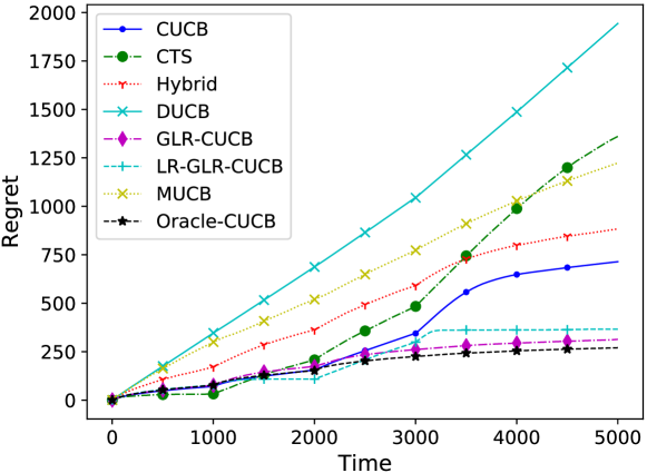
Figure 1: Expected cumulative regret for different algorithms on synthetic dataset.

Note that the optimal super arm does not change for the last three piecewise-stationary segments. Observe that the well-tuned GLR change-point detector is insensitive to change with small magnitude, which implicitly avoids unnecessary and costly global restart, since small change is less likely to affect the optimal super arm. Surprisingly, GLR-CUCB and LR-GLR-CUCB perform nearly as well as Oracle-CUCB and significantly better than other algorithms in regrets. In general, algorithms designed for stochastic CMAB outperform algorithms designed for piecewise-stationary MAB. The reason is when the horizon is small, the dimension of the action space dominates the regret, and this effect becomes more obvious when $m$ is larger. Although order-wise, the cost incurred by the change-point detection is much higher than the cost incurred by exploration.

Note that our experiment on this synthetic dataset does not satisfy Assumption 4.1. For example, the gap between the first segment and second segment is $0.6$, and we choose $\delta=\frac{20}{T}$ and $p=0.05\sqrt{(N-1)\log{T}/T}$ for GLR-CUCB, which means the length of the second segment should be at least 9874. However, the actual length of the second segment is only 1000. Thus our algorithm performs very well compared to other algorithms even if Assumption 4.1 is violated. If Assumption 4.1 is satisfied, GLR-CUCB can only perform better since it is easier to detect the change in distribution.

6.2 Yahoo! Dataset

We adopt the benchmark dataset for the real-world evaluation of bandit algorithms from Yahoo!. This dataset contains user click log for news articles displayed in the Featured Tab of the Today Module (Li et al., 2011). Every base arm corresponds to the click rate of one article. Upon arrival of a user, our goal is to maximize the expected number of clicked articles by presenting $m$ out of $K$ articles to the users.

Yahoo! Experiment 1 ($K=6$, $m=2$, $N=9$).

We pre-process the dataset following Cao et al. (2019). To make the experiment nontrivial, we modify the dataset by: 1) the click rate of each base arm is enlarged by $10$ times; 2) Reducing the time horizon to $T=22500$. Results are in Figure 2.

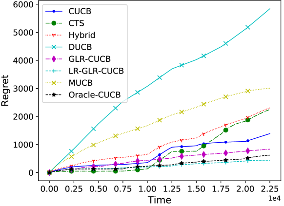
Figure 2: Expected cumulative regret for different algorithms on Yahoo! experiment 1.

Yahoo! experiment 1 is much harder than the synthetic problem, since it is much more non-stationary. Our experiments show GLR-CUCB still significantly outperforms other algorithms and only has a small gap with respect to Oracle-CUCB. Again, Assumption 4.1 does not hold for these two instances, thus we believe it is fair to compare GLR-CUCB with other algorithms. Unexpectedly, LR-GLR-CUCB performs even better than oracle-CUCB, which suggests there is still much to exploit in the piecewise-stationary bandits, since global restart has inferior performance in some cases, especially when the change in distribution is not significant. Additional experiments on Yahoo! dataset can be found in Appendix C.1.

7 Conclusion and Future Work

We have developed the first efficient and general algorithm for piecewise-stationary CMAB, termed GLR-UCB, which extends CUCB (Chen et al., 2013), by incorporating a GLR change-point detector. We analyze the regret upper bound of GLR-CUCB on the order of $\mathcal{O}(\sqrt{NKT\log T})$, and prove the minimax lower bound for piecewise-stationary MAB and CMAB on the order of $\Omega(\sqrt{NKT})$, which shows our algorithm is nearly order-optimal within poly-logarithm factors. Experimental results show our proposed algorithm outperforms other state-of-the art algorithms.

Future work includes designing algorithms for piecewise-stationary CMAB with better restart strategy. GLR-CUCB restarts whenever the GLR change-point detector declares the reward distribution of one base arm changes, but this restart is very likely unnecessary, because change-point with small magnitude might not change the optimal superarm. Another very challenging unsolved problem is whether one can close the gap between the regret upper bound and the minimax regret lower bound. Specifically, develop algorithm which is order-optimal for piecewise-stationary CMAB. It is also important to study other non-stationary settings for combinatorial semi-bandits, such as the dynamic case (with bounded total variation throughout time) (Chen et al., 2020).

Appendices

Appendix A Detailed Proofs of Theorem 4.2

A.1 Proof of Lemma 4.4

Proof.

Define $N_{k}(t)$ as a counter for each base arm $k\in\mathcal{K}$ at time $t$ (note that it is different from the counter $n_{k}$ defined in the algorithm) and update the counters in each round as follows: (1) After the $K$ initialization rounds, set $N_{k}(K)=1,\forall k\in\mathcal{K}$. (2) For a round $t>K$, if $S_{t}$ is bad, then increase $N_{k^{*}}(t)$ by one, where $k^{*}=\arg\min_{k\in\mathcal{K}}N_{k}(t-1)$. By definition, the total number of bad rounds at time $T$ is no more than $\sum_{k\in\mathcal{K}}N_{k}(T)$. Throughout the proof, we will use $n_{k}(t)$ to denote the total number of times arm $k$ is played by the agent till time $t$, to emphasize the time dependency in order to make the proof more readable.
Note that when a bad super arm is played, it incurs loss at most $\Delta^{\text{max},1}_{\textup{opt}}$. Thus,

$$\mathcal{R}(T) \leq\Delta^{\text{max},1}_{\textup{opt}}\mathbb{E}\left[\sum_{k\in\mathcal{K}}N_{k}(T)\right].$$

Thus it suffices to upper bound $\mathbb{E}\left[\sum_{k\in\mathcal{K}}N_{k}(T)\right]$ to upper bound the cumulative regret. Let $l_{t}=\frac{6KL^{2}\log t}{\left(\Delta^{\text{min},1}_{\textup{opt}}\right)^{2}}$, we have

$$\sum_{k\in\mathcal{K}}N_{k}(T)-Kl_{T}=\sum_{k\in\mathcal{K}}N_{k}(T)\mathbb{I}{\{\tau_{1}\leq T\}}+\sum_{k\in\mathcal{K}}N_{k}(T)\mathbb{I}{\{\tau_{1}\geq T\}}-K(l_{T}+1)$$

$$=\sum_{k\in\mathcal{K}}N_{k}(T)\mathbb{I}\left\{\tau_{1}\leq T\right\}+\sum_{t=K+1}^{T}\mathbb{I}\left\{S_{t}\in\mathcal{S}_{B}^{1},\tau_{1}\geq T\right\}-Kl_{T}$$

$$=\sum_{k\in\mathcal{K}}N_{k}(T)\mathbb{I}\left\{\tau_{1}\leq T\right\}+\sum_{t=K+1}^{T}\mathbb{I}\left\{S_{t}\in\mathcal{S}_{B}^{1},\tau_{1}\geq T,t\;\mathrm{mod}\;\left\lfloor\frac{K}{p}\right\rfloor\in\mathcal{K}\right\}+$$

$$\quad\sum_{t=K+1}^{T}\mathbb{I}\left\{S_{t}\in\mathcal{S}_{B}^{1},\tau_{1}\geq T,t\;\mathrm{mod}\;\left\lfloor\frac{K}{p}\right\rfloor\not\in\mathcal{K}\right\}-Kl_{T}$$

$$\leq T\mathbb{I}\left\{\tau_{1}\leq T\right\}+\sum_{t=K+1}^{T}\mathbb{I}\left\{t\;\mathrm{mod}\;\left\lfloor\frac{K}{p}\right\rfloor\in\mathcal{K}\right\}+\sum_{t=K+1}^{T}\sum_{k\in\mathcal{K}}\mathbb{I}\left\{S_{t}\in\mathcal{S}_{B}^{1},N_{k}(t)>N_{k}(t-1),N_{k}(t-1)>l_{T}\right\}$$

$$\leq T\mathbb{I}\left\{\tau_{1}\leq T\right\}+\sum_{t=K+1}^{T}\mathbb{I}\left\{t\;\mathrm{mod}\;\left\lfloor\frac{K}{p}\right\rfloor\in\mathcal{K}\right\}+\sum_{t=K+1}^{T}\sum_{k\in\mathcal{K}}\mathbb{I}\left\{S_{t}\in\mathcal{S}_{B}^{1},N_{k}(t)>N_{k}(t-1),N_{k}(t-1)>l_{t}\right\}$$

$$=T\mathbb{I}\left\{\tau_{1}\leq T\right\}+\sum_{t=K+1}^{T}\mathbb{I}\left\{t\;\mathrm{mod}\;\left\lfloor\frac{K}{p}\right\rfloor\in\mathcal{K}\right\}+\sum_{t=K+1}^{T}\mathbb{I}\left\{S_{t}\in\mathcal{S}_{B}^{1},\forall k\in S_{t},N_{k}(t-1)>l_{t}\right\}$$

$$\leq T\mathbb{I}\left\{\tau_{1}\leq T\right\}+\sum_{t=K+1}^{T}\mathbb{I}\left\{t\;\mathrm{mod}\;\left\lfloor\frac{K}{p}\right\rfloor\in\mathcal{K}\right\}+\sum_{t=K+1}^{T}\mathbb{I}\left\{S_{t}\in\mathcal{S}_{B}^{1},\forall k\in S_{t},n_{k}(t-1)>l_{t}\right\}.$$

The next step is to show $\mathbb{P}\left(S_{t}\in\mathcal{S}_{B}^{1},\forall k\in S_{t},n_{k}(t-1)>l_{t}\right)\leq\frac{2K}{t^{2}},\forall t\in[T]$. Let $n_{k}(t)$ be the number of times arm $k$ is played in the first $t$ rounds, $\hat{\mu}^{1}_{k,m}$ be the empirical mean of $m$ samples of $k$th arm at the first piecewise-stationary segment, $\text{UCB}_{k}(t)$ be the UCB index of $k$th arm at time $t$, and $\mu_{k}^{1}$ be the actual mean of $k$th arm during the first piecewise-stationary segment. For any $k\in\mathcal{K}$, by applying the Hoeffding’s inequality, we have

$$\mathbb{P}\left(\hat{\mu}_{k,n_{k}(t-1)}^{1}-\mu_{k}^{1}\geq\sqrt{\frac{3\log{t}}{2n_{k}(t-1)}}\right)\leq\sum_{m=1}^{t-1}\mathbb{P}\left(\hat{\mu}^{1}_{k,1:m}-\mu_{k}^{1}\geq\sqrt{\frac{3\log{t}}{2m}}\right)\leq te^{-3\log t}=t^{-2}.$$

Define the event $E_{t}=\left\{\forall k\in\mathcal{K},\hat{\mu}^{1}_{k,n_{k}(t-1)}-\mu_{k}^{1}\leq\sqrt{\frac{3\log{t}}{2n_{k}(t-1)}}\right\}$. By the union bound we have $\mathbb{P}\left(\overline{E}_{t}\right)\leq Kt^{-2}$. However, we can show that $E_{t}\cap\left\{S_{t}\in\mathcal{S}_{B}^{1},\forall k\in S_{t},n_{k}(t-1)>l_{t}\right\}=\emptyset$. In other words, these two events are mutually exclusive. The reason is if both of these events hold, we have

$$r_{\boldsymbol{\mu}^{1}}(S_{t})+L\sqrt{K\frac{6\log t}{l_{t}}}\overset{(a)}{>}r_{\boldsymbol{\mu}^{1}}(S_{t})+L\sqrt{K\max_{k\in S_{t}}\frac{6\log t}{n_{k}(t-1)}}\overset{(b)}{\geq}r_{\text{UCB}}(S_{t})\overset{(c)}{\geq}\alpha\max_{\tilde{S}\in\mathcal{F}}r_{\text{UCB}}(\tilde{S})\overset{(d)}{\geq}\alpha\max_{\tilde{S}\in\mathcal{F}}r_{\boldsymbol{\mu}^{1}}(\tilde{S}),$$

where $\boldsymbol{\mu}^{1}$ is the mean vector of the base arms at the first piecewise-stationary segment. As for these above inequalities, (a) holds since $n_{k}(t-1)>l_{t},\forall k\in S_{t}$; (b) holds by the $L$-Lipschitz property of $r_{\mu}(\cdot)$ and $\left\lVert\text{UCB}-\boldsymbol{\mu}^{1}\right\rVert\leq\sqrt{K\max_{k\in S_{t}}\frac{6\log t}{n_{k}(t-1)}}$. Note that the upper bound of the norm of vector difference comes from the fact that $|\hat{\mu}_{k,n_{k}(t-1)}^{1}-\mu_{k}^{1}|\leq\sqrt{\frac{3\log t}{2n_{k}(t-1)}}$, and $\text{UCB}_{k}(t-1)=\hat{\mu}^{1}_{k,n_{k}(t-1)}+\sqrt{\frac{3\log{t}}{2n_{k}(t-1)}}$; (c) holds by the definition of $\alpha$-approximation oracle; (d) holds by the monotone property of $r_{\mu}(\cdot)$ and $\text{UCB}\geq\boldsymbol{\mu}^{1}$. However this contradicts the fact that $r_{\boldsymbol{\mu}^{1}}(S_{t})+L\sqrt{K\frac{6\log t}{l_{t}}}\leq\alpha\max_{\tilde{S}\in\mathcal{F}}r_{\boldsymbol{\mu}^{1}}(\tilde{S})$, since $L\sqrt{K\frac{6\log t}{l_{t}}}=\Delta^{\text{min},1}_{\textup{opt}}$, which implies that these two events are mutually exclusive. Thus,

$$\mathbb{P}\left(S_{t}\in\mathcal{S}_{B},\forall k\in S_{t},n_{k}(t-1)>l_{t}\right)\leq\mathbb{P}\left(\overline{E}_{t}\right)\leq 2Kt^{-2}.$$

To sum up,

$$\mathbb{E}\left[\sum_{k\in\mathcal{K}}N_{k}(T)\right] \leq K(l_{T}+1)+p(T-K)+\sum_{t=K+1}^{T}\mathbb{P}\left(S_{t}\in\mathcal{S}_{B}^{1},\forall k\in S_{t},n_{k}(t-1)>l_{t}\right)+T\mathbb{P}(\tau_{1}\leq T)$$

$$\leq K(l_{T}+1)+pT+\sum_{t=1}^{T}\frac{K}{t^{2}}+T\mathbb{P}(\tau_{1}\leq T)\leq\frac{6L^{2}K^{2}\log T}{(\Delta^{\text{min},1}_{\textup{opt}})^{2}}+pT+\left(\frac{\pi^{2}}{6}+1\right)K+T\mathbb{P}(\tau_{1}\leq T).$$

The proof is done. ∎

A.2 Proof of Lemma 4.5

Proof.

Define $\tau_{k,1}$ as the first change-point detection time of the $k$th base arm, and then $\tau_{1}=\min_{k\in\mathcal{K}}\tau_{k,1}$ as GLR_CUCB restarts the whole algorithm if change-point is detected on any of the base arms. Applying the union bound to the false alarm probability $\mathbb{P}\left(\tau_{1}\leq T\right)$, we have that

$$\mathbb{P}\left(\tau_{1}\leq T\right)\leq\sum_{k=1}^{K}\mathbb{P}\left(\tau_{k,1}\leq\tau\right).$$

Recall the GLR statistic defined in Eq. (1), and substitute it into $\mathbb{P}\left(\tau_{k,1}\leq T\right)$,

$$\mathbb{P}\left(\tau_{k,1}\leq T\right) \leq\mathbb{P}\left[\exists n\leq n_{k}~{}\mbox{and}~{}s<n:s\times\text{kl}\left(\hat{\mu}^{1}_{k,1:s},\hat{\mu}^{1}_{k,1:n}\right)+(n-s)\times\text{kl}\left(\hat{\mu}^{1}_{k,s+1:n},\hat{\mu}^{1}_{k,1:n}\right)>\beta(n,\delta)\right]$$

$$\overset{(a)}{\leq}\mathbb{P}\left[\exists n\leq T~{}\mbox{and}~{}s<n:s\times\text{kl}\left(\hat{\mu}^{1}_{k,1:s},\hat{\mu}^{1}_{k,1:n}\right)+(n-s)\times\text{kl}\left(\hat{\mu}^{1}_{k,s+1:n},\hat{\mu}^{1}_{k,1:n}\right)>\beta(n,\delta)\right]$$

$$\overset{(b)}{\leq}\mathbb{P}\left[\exists n\leq T~{}\mbox{and}~{}s<n:s\times\text{kl}\left(\hat{\mu}^{1}_{k,1:s},\mu_{k}^{1}\right)+(n-s)\times\text{kl}\left(\hat{\mu}^{1}_{k,s+1:n},\mu^{1}_{k}\right)>\beta(n,\delta)\right]$$

$$\overset{(c)}{\leq}\sum_{s=1}^{T}\mathbb{P}\left[\exists s<n:s\times\text{kl}\left(\hat{\mu}^{1}_{k,1:s},\mu_{k}^{1}\right)+(n-s)\times\text{kl}\left(\hat{\mu}^{1}_{k,s+1:n},\mu^{1}_{k}\right)>\beta(n,\delta)\right]$$

$$\leq\sum_{s=1}^{T}\mathbb{P}\left[\exists r\in\mathbb{N}:s\times\text{kl}\left(\hat{\mu}^{1}_{k,1:s},\mu_{k}^{1}\right)+r\times\text{kl}\left(\hat{\mu}^{1}_{k,s+1:s+r},\mu^{1}_{k}\right)>\beta(s+r,\delta)\right]$$

$$\overset{(d)}{\leq}\sum_{s=1}^{T}\frac{\delta}{3s^{3/2}}\overset{(e)}{\leq}\sum_{s=1}^{\infty}\frac{\delta}{3s^{3/2}}\leq\delta,$$

where $\hat{\mu}_{s,s^{\prime}}^{1}$ is the mean of the rewards generated from the distribution $f_{k}^{1}$ with expected reward $\mu_{k}^{1}$ from time step $s$ to $s^{\prime}$ as only stationary scenario is considered here. Here, inequality (a) is because of the fact that $n_{k}\leq T$; inequality (b) holds since:

$$s\times\text{kl}\left(\hat{\mu}_{1:s},\hat{\mu}_{1:n}\right)+(n-s)\times\text{kl}\left(\hat{\mu}_{s+1:n},\hat{\mu}_{1:n}\right)=\inf_{\lambda\in[0,1]}\left[s\times\text{kl}\left(\hat{\mu}_{1:s},\lambda\right)+(n-s)\times\text{kl}\left(\hat{\mu}_{s+1:n},\lambda\right)\right];$$

inequality (c) is because of the union bound; inequality (d) is according to the Lemma 10 in Besson and Kaufmann [2019]; inequality (e) holds due to the Riemann zeta function $\zeta(s)$, when $s=1.5$, $\zeta(s)<2.7$. Summing over $k\in\mathcal{K}$, we conclude that $\mathbb{P}\left(\tau_{1}\leq T\right)\leq K\delta$. ∎

A.3 Proof of Corollary 4.7

Proof.

By the definition of $\mathcal{C}^{(i)}$, it follows directly that the conditional expected detection delay is upper bounded by $d_{i}$. ∎

A.4 Proof of Theorem 4.2

Proof.

Define the good event $F_{i}=\{\tau_{i}>\nu_{i}\}$ and good event $D_{i}=\{\tau_{i}\leq\nu_{i}+d_{i}\}$, $\forall 1\leq i\leq N-1$. Recall the definition of the good event $\mathcal{C}^{(i)}$ that all the change-points up to $i$th one have been detected successfully and efficiently in Eq. (2), and we can find that $\mathcal{C}^{(i)}=F_{1}\cap D_{1}\cap\cdots\cap F_{i}\cap D_{i}$ is the intersection of the event sequence of $F_{i}$ and $D_{i}$ up to the $i$th change-point. By first decomposing the expected $\alpha$-approximation cumulative regret with respect to the event $F_{1}$, we have that

$$\mathcal{R}(T)=\mathbb{E}\left[R(T)\right] =\mathbb{E}\left[R(T)\mathbb{I}{\{F_{1}\}}\right]+\mathbb{E}\left[R(T)\mathbb{I}{\{\overline{F}_{1}\}}\right]$$

$$\leq\mathbb{E}\left[R(T)\mathbb{I}{\{F_{1}\}}\right]+T\Delta^{\text{max}}_{\text{opt}}\mathbb{P}(\overline{F}_{1})$$

$$\leq\mathbb{E}\left[R(\nu_{1})\mathbb{I}{\{F_{1}\}}\right]+\mathbb{E}\left[R(T-\nu_{1})\right]+T\Delta^{\text{max}}_{\text{opt}}K\delta$$

$$\overset{(a)}{\leq}\widetilde{C}_{1}+\Delta^{\text{max},1}_{\text{opt}}\nu_{1}p+\mathbb{E}\left[R(T-\nu_{1})\right]+T\Delta^{\text{max}}_{\text{opt}}K\delta,$$

where $R(t^{\prime})=\alpha\sum_{t=1}^{t^{\prime}}\max_{S\in\mathcal{F}}r_{\bm{\mu}_{t}}(S)-\sum_{t=1}^{t^{\prime}}r_{\bm{\mu}_{t}}(S_{t})$ and $R(t^{\prime\prime}-t^{\prime})=\alpha\sum_{t=t^{\prime}+1}^{t^{\prime\prime}}\max_{S\in\mathcal{F}}r_{\bm{\mu}_{t}}(S)-\sum_{t=t^{\prime}+1}^{t^{\prime\prime}}r_{\bm{\mu}_{t}}(S_{t})$. Here, $\mathbb{P}(\overline{F}_{1})$ enters the equation by Lemma 4.5, and inequality $(a)$ is due to the bound in the Lemma 4.4.

Next, we turn to bounding $\mathbb{E}\left[R(T-\nu_{1})\right]$. By the law of total expectation, we have

$$\mathbb{E}\left[R(T-\nu_{1})\right] \leq\mathbb{E}\left[R(T-\nu_{1})\bigm{|}F_{1}\cap D_{1}\right]+T\Delta^{\text{max}}_{\text{opt}}(1-\mathbb{P}(F_{1}\cap D_{1}))$$

$$=\mathbb{E}\left[R(T-\nu_{1})\bigm{|}F_{1}\cap D_{1}\right]+T\Delta^{\text{max}}_{\text{opt}}\mathbb{P}(\overline{F}_{1}\cup\overline{D}_{1})$$

$$\leq\mathbb{E}\left[R(T-\nu_{1})\bigm{|}F_{1}\cap D_{1}\right]+T\Delta^{\text{max}}_{\text{opt}}(K+1)\delta,$$

where the probability $\mathbb{P}(\overline{F}_{1}\cup\overline{D}_{1})$ is from applying the union bound to Lemma 4.6. Furthermore, notice that

$$\mathbb{E}\left[R(T-\nu_{1})\bigm{|}F_{1}\cap D_{1}\right] =\mathbb{E}\left[R(T-\nu_{1})\bigm{|}\mathcal{C}^{(1)}\right]$$

$$\leq\mathbb{E}\left[R(T-\tau_{1})\bigm{|}\mathcal{C}^{(1)}\right]+E\left[R(\tau_{1}-\nu_{1})\bigm{|}\mathcal{C}^{(1)}\right]$$

$$\leq\mathbb{E}\left[R(T-\nu_{1})\bigm{|}\mathcal{C}^{(1)}\right]+\Delta^{\text{max},2}_{\text{opt}}d_{1},$$

where $\mathbb{E}\left[R(\tau_{1}-\nu_{1})\bigm{|}\mathcal{C}^{(1)}\right]$ is upper-bounded according to Corollary 4.7. By combining the previous steps, we have that

$$\mathcal{R}(T)\leq\mathbb{E}\left[R(T-\nu_{1})\bigm{|}\mathcal{C}^{(1)}\right]+\widetilde{C}_{1}+\Delta^{\text{max},1}_{\text{opt}}\nu_{1}p+\Delta^{\text{max},2}_{\text{opt}}d_{1}+3T\Delta^{\text{max}}_{\text{opt}}K\delta.$$

Similarly,

$$\mathbb{E}\left[R(T-\nu_{1})\bigm{|}\mathcal{C}^{(1)}\right] \leq\mathbb{E}\left[R(T-\nu_{1})\mathbb{I}{\{F_{2}\}}\bigm{|}\mathcal{C}^{(1)}\right]+T\Delta^{\text{max}}_{\text{opt}}\mathbb{P}\left(\overline{F}_{2}\bigm{|}\mathcal{C}^{(1)}\right)$$

$$\leq\mathbb{E}\left[R(\nu_{2}-\nu_{1})\mathbb{I}{\{F_{2}\}}\bigm{|}C^{(1)}\right]+\mathbb{E}\left[R(T-\nu_{2})\bigm{|}\mathcal{C}^{(1)}\right]+T\Delta^{\text{max}}_{\text{opt}}K\delta$$

$$\leq\widetilde{C}_{2}+\Delta^{\text{max},2}_{\text{opt}}(\nu_{2}-\nu_{1})p+\mathbb{E}\left[R(T-\nu_{2})\bigm{|}\mathcal{C}^{(1)}\right]+T\Delta^{\text{max}}_{\text{opt}}K\delta,$$

where $\mathbb{P}\left(\overline{F}_{2}\bigm{|}\mathcal{C}^{(1)}\right)$ directly follows Lemma 4.6. For the term $\mathbb{E}\left[R(T-\nu_{2})\bigm{|}\mathcal{C}^{(1)}\right]$, we further decompose is as follows,

$$\mathbb{E}\left[R(T-\nu_{2})\bigm{|}\mathcal{C}^{(1)}\right] \leq\mathbb{E}\left[R(T-\nu_{2})\bigm{|}F_{2}\cap D_{2}\cap\mathcal{C}^{(1)}\right]+T\Delta^{\text{max}}_{\text{opt}}\left(1-\mathbb{P}\left(F_{2}\cap D_{2}\bigm{|}\mathcal{C}^{(1)}\right)\right)$$

$$=\mathbb{E}\left[R(T-\nu_{2})\bigm{|}F_{2}\cap D_{2}\cap\mathcal{C}^{(1)}\right]+T\Delta^{\text{max}}_{\text{opt}}\mathbb{P}\left(\overline{F}_{2}\cup\overline{D}_{2}\bigm{|}\mathcal{C}^{(1)}\right)$$

$$\leq E\left[R(T-\nu_{2})\bigm{|}\mathcal{C}^{(2)}\right]+T\Delta^{\text{max}}_{\text{opt}}(K+1)\delta,$$

where $\mathbb{P}\left(\overline{F}_{2}\cup\overline{D}_{2}\bigm{|}\mathcal{C}^{(1)}\right)$ follows Lemma 4.6 by applying the union bound. For $\mathbb{E}[R(T-\nu_{2})|\mathcal{C}^{(2)}]$, we have

$$\mathbb{E}\left[R(T-\nu_{2})\bigm{|}\mathcal{C}^{(2)}\right] \leq\mathbb{E}\left[R(T-\tau_{2})|\mathcal{C}^{(2)}\right]+\mathbb{E}\left[R(\tau_{2}-\nu_{2})\bigm{|}\mathcal{C}^{(2)}\right]$$

$$\leq\mathbb{E}\left[R(T-\nu_{2})\bigm{|}\mathcal{C}^{(2)}\right]+\Delta^{\text{max},3}_{\text{opt}}\mathbb{E}\left[\tau_{2}-\nu_{2}\bigm{|}\mathcal{C}^{(2)}\right]$$

$$\leq\mathbb{E}[R(T-\nu_{2})|\mathcal{C}^{(2)}]+\Delta^{\text{max},3}_{\text{opt}}d_{2}.$$

Wrapping up previous steps, we have that

$$\mathcal{R}(T)\leq\mathbb{E}\left[R(T-\nu_{2})\bigm{|}\mathcal{C}^{(2)}\right]+\widetilde{C}_{1}+\widetilde{C}_{2}+\Delta^{\text{max},1}_{\text{opt}}\nu_{1}p+\Delta^{\text{max},2}_{\text{opt}}(\nu_{2}-\nu_{1})p+\Delta^{\text{max},2}_{\text{opt}}d_{1}+\Delta^{\text{max},3}_{\text{opt}}d_{2}+6T\Delta^{\text{max}}_{\text{opt}}K\delta.$$

Recursively, we can bound $E\left[R(T-\nu_{i})\bigm{|}\mathcal{C}^{(i)}\right]$ by applying the same method as before, and the upper bound on the regret of GLR-CUCB is

$$\mathcal{R}(T)\leq\sum_{i=1}^{N}\widetilde{C}_{i}+\Delta^{\text{max}}_{\text{opt}}Tp+\sum_{i=1}^{N-1}\Delta^{\text{max},i+1}_{\text{opt}}d_{i}+3NT\Delta^{\text{max}}_{\text{opt}}K\delta.$$

∎

A.5 Proof of Corollary 4.3

Proof.

Notice that

$$d_{i} =\left\lceil\frac{4K}{p(\Delta_{\textup{change}}^{i})^{2}}\beta(T,\delta)+\frac{K}{p}\right\rceil\leq\frac{4K}{p(\Delta_{\text{change}}^{i})^{2}\beta(T,\delta)}+\frac{2K}{p}$$

$$\overset{(a)}{\leq}\frac{4K}{p(\Delta_{\text{change}}^{i})^{2}}\left[\log(\frac{3T^{3/2}}{\delta})+8\log\left(1+\frac{\log(\frac{3T^{3/2}}{\delta})}{2}+\sqrt{\log(\frac{3T^{3/2}}{\delta}})\right)+6\log(1+\log{T})\right]+\frac{2K}{p}$$

$$\overset{(b)}{\leq}\frac{\frac{20K\log{T}+o(K\log{T})}{(\Delta_{\text{change}}^{i})^{2}}+2K}{p}\lesssim\frac{K\log{T}}{p(\Delta_{\text{change}}^{\text{min}})^{2}},$$

where inequalities $(a)$ and $(b)$ hold when $\log(3T^{5/2})\geq 10$ (equals to $T\geq 36$). By plugging $d_{i}$ into Theorem 4.2, we have,

$$\mathcal{R}(T)\lesssim\frac{NK^{2}\log{T}\Delta^{\text{max}}_{\textup{opt}}}{\left(\Delta^{\text{min}}_{\textup{opt}}\right)^{2}}+\Delta^{\text{max}}_{\text{opt}}Tp+\frac{N\Delta^{\text{max}}_{\text{opt}}K\log{T}}{p(\Delta_{\text{change}}^{\text{min}})^{2}}+3NK\Delta^{\text{max}}_{\text{opt}}.$$

Combining the above analysis we conclude the corollary. ∎

Appendix B Proof of Theorem 5.1

Proof.

Consider a randomized hard instance defined as follows. First partition the decision horizon into $N$ segments, where the first $N-1$ segments are of size $l=\lceil\frac{T}{N}\rceil$, and the last segment’s length is $T-(N-1)l$. Denote these $N$ segments as $\mathcal{B}_{1},\mathcal{B}_{2},...,\mathcal{B}_{N}$. In each segment, assume the rewards of all arms follow Bernoulli distribution. Furthermore, we assume the following

• $\mu_{k}^{t_{1}}=\mu_{k}^{t_{2}}$, $\forall k\in\mathcal{K}$ and $t_{1},t_{2}\in\mathcal{B}_{i}$ for some $i\in[N]$ (Here, with a little inconsistency with the previous notation, $\mu_{k}^{t}$ is the mean of the reward of arm $k$ at time $t$).

• $\mu_{k}^{t}\in\{\frac{1}{2},\frac{1}{2}+\epsilon\}$, $\forall k\in\mathcal{K}$ and $\forall t\in\mathcal{T}$, where $\epsilon$ is a parameter that needs to be tuned later.

• $\sum_{i=1}^{K}\mu_{i}^{t}=\frac{K}{2}+\epsilon$, $\forall t\in\mathcal{T}$.

Basically at each time instant there is an optimal arm with expected reward $\frac{1}{2}+\epsilon$, and the rest of the base arms have the same reward $\frac{1}{2}$. In addition, in each segment, the reward distribution of all arms stay unchanged. Lastly, we need to specify how the reward distributions change in the consecutive blocks. In $B_{i}$ if the optimal arm is $k_{i}^{*}$, then the optimal arm in $B_{i+1}$ will be drawn uniformly at random from $\mathcal{K}\setminus k_{i}^{*}$.

Now we finish setting up the randomized piecewise-stationary bandit instance. To prove the theorem, we need some more notations. Fix a policy $\pi$, and fix a segment $i\in[N]$, let $k_{i}^{*}$ denote the best arm in that segment. We denote by $P_{k_{i}^{*}}^{i}$ the probability distribution conditioned on arm $k_{i}^{*}$ being the best arm in segment $i$, and by $P_{0}$ the probability distribution with respect to non-optimal rewards for each arm, i.e. with expected reward $\frac{1}{2}$. Furthermore, we denote by $\mathbb{E}_{k_{i}^{*}}^{i}[\cdot]$ and $\mathbb{E}_{0}[\cdot]$ the respective expectations. Lastly, $N_{k}^{i}$ is the number of times arm $k$ was selected in segment $i$ and $X\in\{0,1\}^{T}$ is the binary reward sequence. To prove the theorem, we need Lemma A.1 in Auer et al. [2002b], which we state for completeness.

Lemma B.1.

(Lemma A.1 in Auer et al. [2002b]) Let $f:\{0,1\}^{T}\rightarrow[0,M]$ be any bounded function defined on reward sequence $X$, then $\forall k\in\mathcal{K}$,

$$\mathbb{E}_{k}^{i}[f(X)]\leq\mathbb{E}_{0}[f(X)]+\frac{T}{2}\sqrt{D_{KL}(P_{0}||P_{k}^{i})\mathbb{E}_{0}[N_{k_{i}^{*}}^{i}]}.$$

Applying the above lemma with $f(X)=N_{k_{i}^{*}}^{i}$, we have

$$\mathbb{E}_{k_{i}^{*}}^{i}[N_{k_{i}^{*}}^{i}]\leq\mathbb{E}_{0}[N_{k_{i}^{*}}^{i}]+\frac{|\mathcal{B}_{i}|}{2}\sqrt{\log{\frac{1}{1-4\epsilon^{2}}}\mathbb{E}_{0}[N_{k_{i}^{*}}^{i}]}.$$

Summing over all arms, we have

$$\sum_{k_{i}^{*}=1}^{K}\mathbb{E}_{k_{i}^{*}}^{i}[N_{k_{i}^{*}}^{i}] \leq\sum_{k_{i}^{*}=1}^{K}\mathbb{E}_{0}[N_{k_{i}^{*}}^{i}]+\sum_{k_{i}^{*}=1}^{K}\frac{|\mathcal{B}_{i}|}{2}\sqrt{\log{\frac{1}{1-4\epsilon^{2}}}\mathbb{E}_{0}[N_{k_{i}^{*}}^{i}]}$$

$$\leq|\mathcal{B}_{i}|+\frac{|\mathcal{B}_{i}|}{2}\sqrt{|\mathcal{B}_{i}|K\log{\frac{1}{1-4\epsilon^{2}}}},$$ (3)

where the last equality holds since $\sum_{k_{i}^{*}=1}^{K}\mathbb{E}_{0}[N_{k_{i}^{*}}^{i}]=|\mathcal{B}_{i}|$ and Jensen’s inequality. Then we can lower bound the regret for any policy $\pi$ for this randomized hard instance. Let $\mathcal{R}^{\pi}_{T}$ be the regret of policy $\pi$ with horizon $T$, we have,

$$\mathcal{R}^{\pi}(T) =(\tfrac{1}{2}+\epsilon)T-\mathbb{E}_{\pi}[\sum_{t=1}^{T}\mu_{t}]$$

$$\geq(\tfrac{1}{2}+\epsilon)T-(\tfrac{1}{2}+\epsilon)\tfrac{1}{K-1}\sum_{i=1}^{N}\sum_{k_{i}^{*}=1}^{K}\mathbb{E}_{k_{i}^{*}}^{i}[N_{k_{i}^{*}}^{i}]-\tfrac{1}{2}(T-\tfrac{1}{K-1}\sum_{i=1}^{N}\sum_{k_{i}^{*}=1}^{K}\mathbb{E}_{k_{i}^{*}}^{i}[N_{k_{i}^{*}}^{i}])$$

$$=\epsilon(T-\tfrac{1}{K-1}\sum_{i=1}^{N}\sum_{k_{i}^{*}=1}^{K}\mathbb{E}_{k_{i}^{*}}^{i}[N_{k_{i}^{*}}^{i}])$$

$$\overset{(a)}{\geq}\epsilon(T-\tfrac{1}{K-1}(\sum_{i=1}^{N}|\mathcal{B}_{i}|+\frac{|\mathcal{B}_{i}|}{2}\sqrt{K|\mathcal{B}_{i}|\log{\tfrac{1}{1-4\epsilon^{2}}}}))$$

$$=\epsilon T-\tfrac{\epsilon T}{K-1}-\tfrac{\epsilon T}{2(K-1)}\sqrt{\frac{KT}{N}\log{\tfrac{1}{1-4\epsilon^{2}}}}$$

$$\overset{(b)}{\geq}\tfrac{\epsilon T}{2}-\tfrac{\epsilon^{2}T}{K-1}\sqrt{\tfrac{KT}{N}\log{\tfrac{4}{3}}}.$$

where $(a)$ is due to inequality (3), and $(b)$ holds by $K\geq 3$, $4\epsilon^{2}\leq\frac{1}{4}$ and $\log{\frac{1}{1-x}}\leq 4\log(\frac{4}{3})x$ for all $x\in[0,\frac{1}{4}]$. We finish the proof by setting $\epsilon=\frac{K-1}{4\sqrt{TK\log{(\frac{4}{3})}}}$. ∎

Appendix C Supplementary Materials for Experiments

C.1 Additional Experimental Results

Reward distributions of base arms along time for three experiments are summarized in Figure 3.

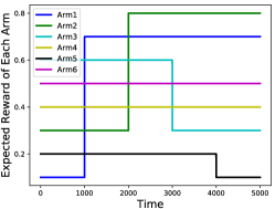
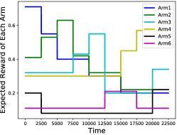
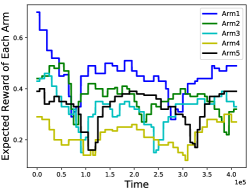
Figure 3: Reward distributions of base arms for all experiments. Left: synthetic data. Middle: Yahoo! experiment 1. Right: Yahoo! experiment 2.

We also run all algorithms on a much harder problem, by extracting the experiment data from Yahoo! dataset following Liu et al. [2018]. Again, to make the experiment nontrivial, we enlarge the click rate of each base arm by $10$ times but the time horizon $T=410000$ is kept. The result is summarized in Figure 4.

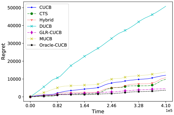
Figure 4: Expected cumulative regret for different algorithms on Yahoo! experiment2.

Lastly, we provide the standard deviation of the last step of all algorithms for different experiments, as shown in Table 1.

	CUCB	CTS	Hybrid	DUCB	GLR-CUCB	LR-GLR-CUCB	MUCB	Oracle-CUCB
Synthetic Dataset	241.08	351.12	278.82	14.08	37.96	73.30	171.45	25.54
Yahoo! Experiment 1	510.20	513.41	826.01	25.44	62.76	63.37	202.44	35.08
Yahoo! Experiment 2	563.54	562.24	1189.17	158.27	517.13	NA	1427.28	160.76

Table 1: Standard deviations of all algorithms for experiments on synthetic and Yahoo! datasets

C.2 Implementation Details

To guarantee the reproducibility of our experiments, we include our choices of parameters of all algorithms for different experiments. Only CUCB, CTS and Oracle-CUCB do not have any parameters to be tuned.
Hybrid: $\gamma$ is set to be 1 for all three experiments.
DUCB: $\gamma=1-\sqrt{1/T}/4$ and $\xi=0.5$ for all experiments on synthetic and Yahoo! datasets.
MUCB: $w=150,500,1500$ for synthetic experiment, Yahoo! experiment 1 and Yahoo! experiment 2, respectively; $b=\sqrt{\frac{w}{2}\log(2|\mathcal{F}|T^{2})},\gamma=0.05\sqrt{(N-1)|\mathcal{F}|(2b+3\sqrt{w})/(2T)}$ for all all experiments on synthetic and Yahoo! datasets.
GLR-CUCB: $\delta=\frac{20}{T}$ for experiment on the synthetic dataset, $\delta=\frac{50}{T}$ for Yahoo! experiment 1, and $\delta=\frac{70}{T}$ for Yahoo! experiment 2. $p=0.05\sqrt{(N-1)\log{T}/T}$ for all experiments on synthetic and Yahoo! datasets.

References

- Agrawal and Goyal [2012] Shipra Agrawal and Navin Goyal. Analysis of Thompson sampling for the multi-armed bandit problem. In Proc. 25th Conf. on Learn. Theory (COLT ’12), pages 1–26, 2012.
- Auer et al. [2002a] Peter Auer, Nicolo Cesa-Bianchi, and Paul Fischer. Finite-time analysis of the multiarmed bandit problem. Mach. Learn., 47(2-3):235–256, 2002a.
- Auer et al. [2002b] Peter Auer, Nicolo Cesa-Bianchi, Yoav Freund, and Robert E Schapire. The nonstochastic multiarmed bandit problem. SIAM J. Comput., 32(1):48–77, 2002b.
- Auer et al. [2019] Peter Auer, Pratik Gajane, and Ronald Ortner. Adaptively tracking the best bandit arm with an unknown number of distribution changes. In Proc. 32nd Conf. on Learn. Theory (COLT ’19), pages 138–158, 2019.
- Ausiello et al. [1995] Giorgio Ausiello, Pierluigi Crescenzi, and Marco Protasi. Approximate solution of NP optimization problems. Theor. Comput. Sci., 150(1):1–55, 1995.
- Basseville and Nikiforov [1993] Michèle Basseville and Igor V Nikiforov. Detection of abrupt changes: theory and application, volume 104. Prentice Hall Englewood Cliffs, 1993.
- Besbes et al. [2014] Omar Besbes, Yonatan Gur, and Assaf Zeevi. Stochastic multi-armed-bandit problem with non-stationary rewards. In Proc. 24th Annu. Conf. Neural Inf. Process. Syst. (NeurIPS ’14), pages 199–207, 2014.
- Besson and Kaufmann [2019] Lilian Besson and Emilie Kaufmann. The generalized likelihood ratio test meets klucb: an improved algorithm for piece-wise non-stationary bandits. arXiv preprint arXiv:1902.01575, 2019.
- Bubeck and Cesa-Bianchi [2012] Sébastien Bubeck and Nicolo Cesa-Bianchi. Regret analysis of stochastic and nonstochastic multi-armed bandit problems. Foundations and Trends in Machine Learning, 5(1):1–122, 2012.
- Bubeck et al. [2018] Sébastien Bubeck, Michael Cohen, and Yuanzhi Li. Sparsity, variance and curvature in multi-armed bandits. In Proc. 29th Int. Conf. Algorithmic Learning Theory(ALT ’18), pages 111–127, 2018.
- Cao et al. [2015] Wei Cao, Jian Li, Yufei Tao, and Zhize Li. On top-k selection in multi-armed bandits and hidden bipartite graphs. In Proc. 29th Annu. Conf. Neural Inf. Process. Syst. (NeurIPS ’15), pages 1036–1044, 2015.
- Cao et al. [2019] Yang Cao, Zheng Wen, Branislav Kveton, and Yao Xie. Nearly optimal adaptive procedure with change detection for piecewise-stationary bandit. In Proc. 22nd Int. Conf. Artif. Intell. Stat. (AISTATS 2019), pages 418–427, 2019.
- Cappé et al. [2013] Olivier Cappé, Aurélien Garivier, Odalric-Ambrym Maillard, Rémi Munos, Gilles Stoltz, et al. Kullback–leibler upper confidence bounds for optimal sequential allocation. Ann. Stat., 41(3):1516–1541, 2013.
- Chen et al. [2013] Wei Chen, Yajun Wang, and Yang Yuan. Combinatorial multi-armed bandit: General framework and applications. In Proc. 30th Int. Conf. Mach. Learn. (ICML 2013), pages 151–159, 2013.
- Chen et al. [2020] Wei Chen, Liwei Wang, Haoyu Zhao, and Kai Zheng. Combinatorial semi-bandit in the non-stationary environment. arXiv preprint arXiv:2002.03580, 2020.
- Combes et al. [2015] Richard Combes, Mohammad Sadegh Talebi Mazraeh Shahi, Alexandre Proutiere, et al. Combinatorial bandits revisited. In Proc. 29th Annu. Conf. Neural Inf. Process. Syst. (NeurIPS ’15), pages 2116–2124, 2015.
- Garivier and Moulines [2011] Aurélien Garivier and Eric Moulines. On upper-confidence bound policies for switching bandit problems. In Proc. 22th Int. Conf. Algorithmic Learning Theory(ALT ’11), pages 174–188. Springer, 2011.
- Hartland et al. [2007] Cédric Hartland, Nicolas Baskiotis, Sylvain Gelly, Michèle Sebag, and Olivier Teytaud. Change point detection and meta-bandits for online learning in dynamic environments. CAp, pages 237–250, 2007.
- Hassan and Curry [2014] Umair Ul Hassan and Edward Curry. A multi-armed bandit approach to online spatial task assignment. In IEEE 11th Intl Conf Ubiquitous Intell. Comput. (UIC ’14), pages 212–219. IEEE, 2014.
- Hazan [2016] Elad Hazan. Introduction to online convex optimization. Foundations and Trends in Optimization, 2(3-4):157–325, 2016.
- Hazan and Kale [2011] Elad Hazan and Satyen Kale. Better algorithms for benign bandits. J. Mach. Learn. Res., 12:1287–1311, Apr 2011.
- Kaufmann and Koolen [2018] Emilie Kaufmann and Wouter Koolen. Mixture martingales revisited with applications to sequential tests and confidence intervals. arXiv preprint arXiv:1811.11419, 2018.
- Kocsis and Szepesvári [2006] Levente Kocsis and Csaba Szepesvári. Discounted UCB. In 2nd PASCAL Challenges Workshop, volume 2, 2006.
- Kveton et al. [2015] Branislav Kveton, Zheng Wen, Azin Ashkan, and Csaba Szepesvari. Tight regret bounds for stochastic combinatorial semi-bandits. In Proc. 18th Int. Conf. Artif. Intell. Stat. (AISTATS 2015), pages 535–543, 2015.
- Lai and Robbins [1985] Tze Leung Lai and Herbert Robbins. Asymptotically efficient adaptive allocation rules. Adv. Appl. Math., 6(1):4–22, 1985.
- Lattimore and Szepesvári [2018] Tor Lattimore and Csaba Szepesvári. Bandit algorithms. preprint, 2018.
- Li et al. [2019] Bingcong Li, Tianyi Chen, and Georgios B Giannakis. Bandit online learning with unknown delays. In Proc. 22th Int. Conf. Artif. Intell. Stat. (AISTATS 2019), pages 993–1002, 2019.
- Li et al. [2011] Lihong Li, Wei Chu, John Langford, and Xuanhui Wang. Unbiased offline evaluation of contextual-bandit-based news article recommendation algorithms. In Proc. 4th ACM Int. Conf. Web Search Data Min. (WSDM ’11), pages 297–306. ACM, 2011.
- Li et al. [2016] Shuai Li, Alexandros Karatzoglou, and Claudio Gentile. Collaborative filtering bandits. In Proc. 39th Annu. Int. ACM SIGIR Conf. Res. Dev. Inf. Retrieval (SIGIR ’16), pages 539–548. ACM, 2016.
- Liu et al. [2018] Fang Liu, Joohyun Lee, and Ness Shroff. A change-detection based framework for piecewise-stationary multi-armed bandit problem. In Proc. 32nd AAAI Conf. Artif. Intell., 2018.
- Mellor and Shapiro [2013] Joseph Mellor and Jonathan Shapiro. Thompson sampling in switching environments with bayesian online change detection. In Proc. 16th Int. Conf. Artif. Intell. Stat. (AISTATS 2013), pages 442–450, 2013.
- Pereira et al. [2018] Fabíola SF Pereira, João Gama, Sandra de Amo, and Gina MB Oliveira. On analyzing user preference dynamics with temporal social networks. Mach. Learn., 107(11):1745–1773, 2018.
- Siegmund [2013] David Siegmund. Sequential analysis: tests and confidence intervals. Springer Science & Business Media, 2013.
- Tang et al. [2013] Liang Tang, Romer Rosales, Ajit Singh, and Deepak Agarwal. Automatic ad format selection via contextual bandits. In Proc. 22nd ACM Int. Conf. Inf. Knowl. Manage. (CIKM ’13), pages 1587–1594. ACM, 2013.
- Thompson [1933] William R Thompson. On the likelihood that one unknown probability exceeds another in view of the evidence of two samples. Biometrika, 25(3/4):285–294, 1933.
- Vempaty et al. [2014] Aditya Vempaty, Lav R Varshney, and Pramod K Varshney. Reliable crowdsourcing for multi-class labeling using coding theory. IEEE J. Sel. Topics Signal Process., 8(4):667–679, 2014.
- Wang and Chen [2018] Siwei Wang and Wei Chen. Thompson sampling for combinatorial semi-bandits. In Proc. 35th Int. Conf. Mach. Learn. (ICML 2018), pages 5114–5122, 2018.
- Wei and Srivatsva [2018] Lai Wei and Vaibhav Srivatsva. On abruptly-changing and slowly-varying multiarmed bandit problems. In Proc. Am. Contr. Conf. (ACC 2018), pages 6291–6296. IEEE, 2018.
- Yu and Mannor [2009] Jia Yuan Yu and Shie Mannor. Piecewise-stationary bandit problems with side observations. In Proc. 26th Int. Conf. Mach. Learn. (ICML 2009), pages 1177–1184. ACM, 2009.
- Zimmert et al. [2019] Julian Zimmert, Haipeng Luo, and Chen-Yu Wei. Beating stochastic and adversarial semi-bandits optimally and simultaneously. In Proc. 36th Int. Conf. Mach. Learn. (ICML 2019), pages 7683–7692, 2019.