ALMA observations of fragmentation, sub-structure, and protostars in high-mass starless clump candidates
Abstract
The initial physical conditions of high-mass stars and protoclusters remain poorly characterized. To this end we present the first targeted ALMA Band 6 continuum and spectral line survey towards high-mass starless clump candidates, selecting a sample of 12 of the most massive candidates () within . The joint array maps have a high spatial resolution of (, ) and have high point source mass-completeness down to at (or column density sensitivity of ). We discover previously undetected signposts of low-luminosity star formation from \ceCO and \ceSiO bipolar outflows towards 11 out of 12 clumps, showing that current MIR/FIR Galactic Plane surveys are incomplete to low- and intermediate-mass protostars (), and emphasizing the necessity of high-resolution followup. We compare a subset of the observed cores with a suite of radiative transfer models of starless cores. We find a high-mass starless core candidate with a model-derived mass consistent with when integrated over size scales of . Unresolved cores are poorly fit by radiative transfer models of externally heated Plummer density profiles, supporting the interpretation they are protostellar even without detection of outflows. A high degree of fragmentation with rich sub-structure is observed towards 10 out of 12 clumps. We extract sources from the maps using a dendrogram to study the characteristic fragmentation length scale. Nearest neighbor separations when corrected for projection with Monte Carlo random sampling are consistent with being equal to the clump average thermal Jeans length (; i.e., separations equal to ). In context of previous observations that on larger scales see separations consistent with the turbulent Jeans length or the cylindrical thermal Jeans scale (), our findings support a hierarchical fragmentation process, where the highest density regions are not strongly supported against thermal gravitational fragmentation by turbulence or magnetic fields.
tablenum \restoresymbolSIXtablenum
1 Introduction
High-mass stars () strongly influence the evolution of galaxies and the ISM, yet many fundamental questions remain to be answered concerning the incipient phases of high-mass star formation (e.g., Beuther et al., 2007; Tan et al., 2014; Motte et al., 2017). Observational constraints on the initial physical conditions of protocluster evolution are a necessary prerequisite to improved understanding of high-mass star and cluster formation. Of particular importance are observations of the quiescent environments before the initial conditions are disrupted by the extreme radiative and mechanical feedback of high-mass stars. Thus our understanding of both how cluster formation is initiated and the ensuing protocluster evolution depend on identifying and constraining the physical properties of representative samples of starless molecular cloud “clumps”111 In this paper we use the term “core” to refer to a dense gas structure that is in size and likely to form a single or bound multiple stellar system. Such cores are embedded within larger scale “clumps” that are dense gas structures likely to form a stellar association or cluster, and are in size and in mass (c.f. Bergin & Tafalla, 2007). .
Recent blind surveys of dust continuum emission at (sub-)millimeter and far-infrared (FIR) wavelengths of the Galactic Plane have identified large statistical samples of clumps, enabling the discovery of those in the earliest evolutionary phases. Such surveys include the Bolocam Galactic Plane Survey222Data products can be downloaded from https://irsa.ipac.caltech.edu/data/BOLOCAM_GPS/ (BGPS; Aguirre et al., 2011; Rosolowsky et al., 2010; Ginsburg et al., 2013) at , ATLASGAL333http://www3.mpifr-bonn.mpg.de/div/atlasgal/ at (Schuller et al., 2009; Contreras et al., 2013; Csengeri et al., 2014), JCMT Galactic Plane Survey444http://apps.canfar.net/storage/list/JPSPR1 at (Eden et al., 2017, JPS), and Herschel Hi-GAL at 70, 160, 250, 350, and (Molinari et al., 2010, 2016). Starless clump candidates (SCCs) are identified by cross-matching clump catalogs to catalogs of star formation indicators and selecting clumps unassociated with any indicators. These indicators include compact sources, color-selected young stellar objects (YSOs), \ceH2O and \ceCH3OH masers, and UCHii regions in Svoboda et al. (2016) for the BGPS and in Yuan et al. (2017) for ATLASGAL, in total identifying more than SCCs in the inner-Galaxy. In addition, more than clumps without sources have been identified from the Hi-GAL survey (Traficante et al., 2015; Elia et al., 2017). In this study we aim to systematically study a representative sample of the highest mass SCCs within in order to understand the fragmentation characteristics at high-spatial resolution, identify potential high-mass starless cores (, ), and search for previously undetected low luminosity protostellar activity.
A variety of physics, including thermal gas pressure, turbulence, magnetic fields, and the geometry of filaments and density gradients, likely play a role in the fragmentation of molecular clouds and the resultant dense core populations. Recent high-resolution observations with millimeter and sub-millimeter interferometers of high-mass clumps with little sign of star formation reveal significant fragmentation at the early stage of cluster formation (Zhang et al., 2009; Zhang & Wang, 2011; Wang et al., 2011, 2012, 2014; Zhang et al., 2015; Lu et al., 2015; Beuther et al., 2015a; Sanhueza et al., 2017). These studies found that the most massive fragments in the clumps are at least ten times greater than the thermal Jeans mass, indicating that additional support from turbulence and/or magnetic fields are required. Most of these studies focused on individual clumps and typically have not had the sensitivity to adequately detect fragments of a thermal Jeans mass (detections of at ). In contrast, the fragmentation scales in nearby molecular clouds have been studied extensively with recent notable analyses towards Serpens (Friesen et al., 2017), Orion Integral Shaped Filament (Kainulainen et al., 2017), and Perseus (Pokhrel et al., 2018). These studies find support for hierarchical, scale-dependent fragmentation with separations corresponding to a range between thermal Jeans fragmentation and thermal filamentary gravitational fragmentation. It is not understood how these results extend towards earlier evolutionary stages in massive SCCs which are the focus of this work.
Publicly available millimeter and FIR Galactic Plane survey observations do not have sufficient angular resolution at ( at ) to study the sub-structure and dense core properties in distant SCCs. The high-mass pre-stellar core candidate G028-C1S () studied in Tan et al. (2013) for example was only identified as protostellar until interferometric followup of outflow tracers (Tan et al., 2016; Feng et al., 2016a). High-mass SCCs remain largely unstudied at high-spatial resolution owing to their historical difficulty in identification and typically large heliocentric distances, with only a handful of studies on individual objects to date (Beuther et al., 2015b; Sanhueza et al., 2017). In particular the high-mass starless clump candidate “MM1” of IRDC G28.23–0.19 (Sanhueza et al., 2013) has been studied in detail to determine that it is devoid of star formation indicators, including point sources, and masers (Wang et al., 2006; Chambers et al., 2009), and radio continuum (Battersby et al., 2010; Rosero et al., 2016). The global physical properties of G28.23–0.19 MM1 (corresponding to BGPS catalog clump number 4649) are similar to the average properties of the SCCs presented in this work. G28.23–0.19 MM1 is high-mass, cold, compact, and dense (i.e., , , , ; Sanhueza et al. 2017). However the sensitivity and sample size of dense cores are not sufficient for a precise measurement of the fragmentation scale, and represents only a single clump. In this survey we present observations on a sample of clumps that are selected from a blind Galactic Plane survey and are among the most massive SCCs.
Existing large samples of SCCs have been primarily identified through the non-detection of coincident Hi-GAL sources (Veneziani et al., 2013; Traficante et al., 2015; Svoboda et al., 2016; Elia et al., 2017) which is less affected than shorter wavelength or observations by both local extinction and from contamination of evolved stars (principally those on the asympototic giant branch). The completeness of the maps to protostar bolometric luminosity, , is affected by the survey depth and complex structure in the foreground and background emission which hinders the clear identification of compact sources. Svoboda et al. (2016) calculate the completeness function for Hi-GAL compact sources associated to BGPS clumps and the respective distribution of heliocentric distances and find that for clumps with low backgrounds () the completeness limit is (see §3.2.4 in Svoboda et al., 2016), which is greater than of YSOs in the Gould’s Belt (n.b. median ; Dunham et al., 2014). Faint sources coincident with the clump column density peaks towards of dark SCCs suggest likely embedded intermediate-mass star formation that is undetected in the Hi-GAL observations (Traficante et al., 2017). However, it is currently unknown what degree of star formation has initiated, if at all, in SCCs without sensitive and unambiguous tracers of protostellar activity such as bipolar molecular outflows. Systematic observations of SCCs at high-resolution are necessary to determine what degree (if any) of low-luminosity star formation has begun in SCCs, with important implications for the protostellar accretion history.
The principal theories of high-mass star formation in dense Galactic molecular cloud clumps are the monolithic collapse of turbulent cores in virial equilibrium (McKee & Tan, 2002, 2003; Hosokawa & Omukai, 2009) and the accretion of sub-virial cores through gravitionally-driven cloud inflow (Smith et al., 2009; Hartmann et al., 2012). The latter replace the competitive Bondi-Hoyle accretion of cores (Bonnell et al., 2001; Wang et al., 2010) with cores fed the gas reservoir through inflowing streams. The turbulent core model predicts monolithic high-mass starless cores whereas the competitive model predicts a fragmentation of cores near the thermal Jeans mass. The existence of high-mass starless cores is a key distinction between these models, yet few, if any, observational candidates are known (Kong et al., 2017), and some promising candidates have revealed embedded protostellar activity upon further observational investigation (i.e. G028-C1S Tan et al., 2013, 2016; Feng et al., 2016b). Irrespective of the specific theoretical model, measurements of the fragmentation properties at early evolutionary phases provide valuable observational constraints on the initial physical conditions of high-mass star and cluster formation. To this end, we perform a systematic search for high-mass starless cores towards massive SCCs with the Atacama Large Millimeter/submillimeter Array.
In this paper we present a systematic survey of high-mass SCCs at sub-arcsecond resolution. We present our sample selection, observational setup, and data reduction methodology in Section 2. We describe detections of previously unknown, low-luminosity protostellar activity in Section 3 and the modeling of continuum sources in Section 4. We measure and analyze the fragmentation scale between sources in Section 5, discuss the implications in Section 6, and report our conclusions in Section 7. In Appendix C we include a detailed description of the setup and computation of radiative transfer models analyzed in Section 4.
2 Observations
2.1 Sample Selection
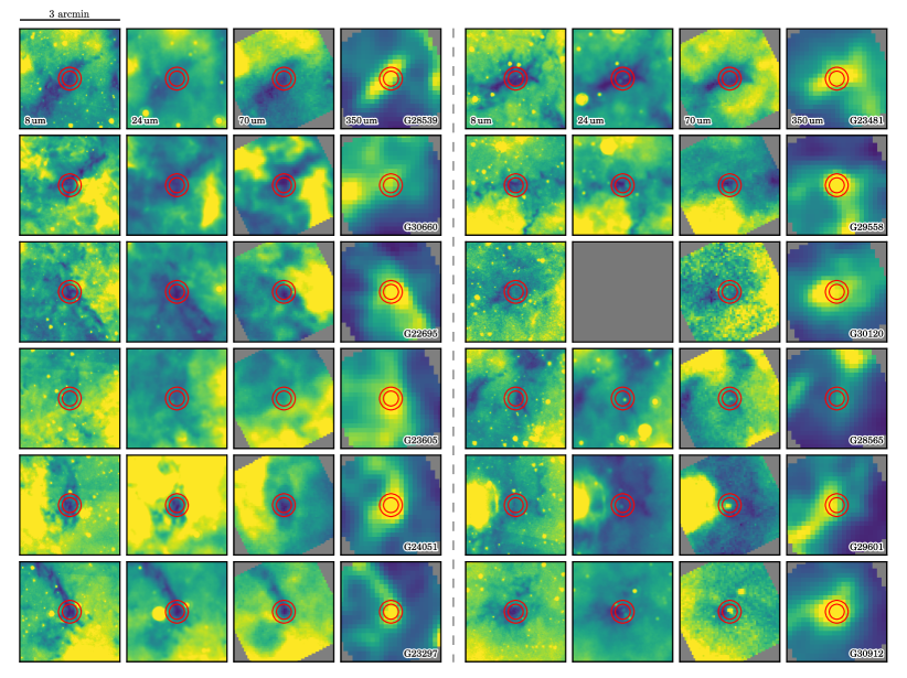
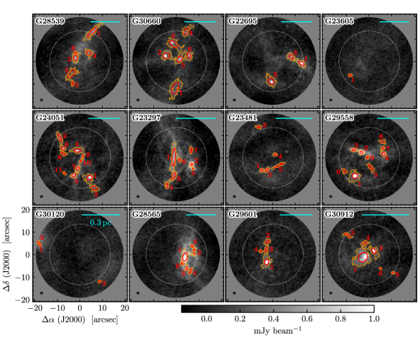
We have identified SCCs through the combined catalogs and images of primarily two dust continuum Galactic Plane surveys: (1) an evolutionary analysis of BGPS (Svoboda et al., 2016, hereafter S16), and (2) comparison of the Peretto & Fuller (2009) infrared dark cloud (IRDC) catalog with Hi-GAL images (Traficante et al., 2015). The BGPS observed between with (expanding to for selected ) at with a synthesized angular resolution. In the region the BGPS has been compared to a diverse set of a observational indicators for star formation activity (S16). These indicators include compact sources, mid-IR color-selected YSOs, \ceH2O masers, Class II \ceCH3OH masers, extended outflows, and UCHii regions. From the sample of more than SCCs in the combined samples of S16 and Traficante et al. (2015), we target the highest mass SCCs within . Point sources at were identified by visual inspection in S16 and by an automated extraction in Traficante et al. (2015). Three clumps (G28565, G29601, and G309120 which were initially determined from the automated extraction to be dark at , upon closer scrutiny by visual inspection show association to weak sources. Among the 12 ALMA targets, nine have no detectable point source emission from Hi-GAL (flag 0 in S16), two have low-confidence or marginal detections (flag 4, G28565 & G29601), and one has bright, compact detection (flag 1, source G30912). We emphasize that starless clump candidates are designated based on the observational data sets and identification techniques used, and that these factors are reflected in the completeness and purity of the resulting catalogs of SCCs. Table 1 details the target positions and velocities. Table 2 details the physical properties of the sample and Figure 1 shows images of the clumps at wavelengths from to .
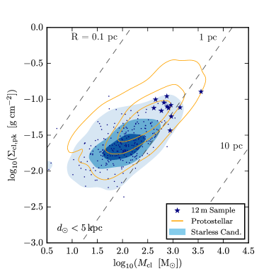
The clump average physical properties in S16 are shown in Figure 2, plotting peak mass surface density (at ) and total mass , for sources with well-constrained distances less than and . Protostellar clumps and SCCs are plotted, where SCCs have quiescent background emission and no detected compact sources from the Hi-GAL images (flag 0, see S16 §3.2.4). Protostellar clumps are typically higher in both mass and mass surface density compared to SCCs. The ALMA targets are shown, occupying the highest and portions of the SCC distribution where typical values for the sample are and (measured over scales). G28539 in particular stands out as the most massive clump in the sample at and also the highest peak mass surface density.
Assuming a star-formation efficiency of and a standard stellar initial mass function (IMF; Kroupa, 2001), a clump meets the criteria of forming a star (see S16 §6.1). All of the clumps that comprise this sample are above this mass threshold, and are similarly above the mass-radius relationship for high-mass star formation proposed by (Kauffmann & Pillai, 2010)555Kauffmann & Pillai (2010) define the prescription for a clump to form high-mass stars. The pre-factor has been scaled for consistency with the dust opacity used in this work. For radius , this relation yields a mass threshold of .. However in practice it is difficult to assess the high-mass star formation potential of clumps beyond these simple heuristics. It should be kept in mind that if the star formation efficiency of the targets is substantially lower than the typical assumed value of then they are unlikely to form high-mass stars.
2.2 ALMA Band 6
As part of Atacama Large Millimeter/submillimeter Array666ALMA is operated by the National Radio Astronomy Observatory, which is a facility of the National Science Foundation, operated under cooperative agreement by Associated Universities, Inc. (ALMA) Cycle 3 program 2015.1.00959.S, we observed 12 clumps in Band 6 in a compact configuration (C36-2; joint array baselines range from ). Data were taken between March, 2016, for the array and between 30 April to 19 August, 2016, for the array. Including time for calibration and overheads, the array observations lasted for approximately , with typical precipitable water vapor of . Titan and J1733–1304 were used as flux calibrators, J1751+0939 to calibrate the bandpass, and J1743–0350 and J1830+0619 to calibrate the time-dependent gains. Identical scheduling blocks were configured to interleave and observe all 12 targets within the same block, and because sources are within a radius on the sky (), the same calibrators can be used. Thus due to nearly identical observing conditions, the individual maps have similar -coverage, atmospheric noise, and beam size.
Positions for the sample were chosen from the BGPS continuum peak flux density position, and compared for consistency with the ATLASGAL peak emission and Hi-GAL peak absorption (when present) positions. The Band 6 receiver was configured in dual-polarization mode with lower and upper sidebands centered near 215 and , respectively. The observations targeted each clump peak with a single pointing with half-power beam width (HPBW) of the measured primary beam ( at ) and 20%-power beam width of (), the effective limit of the array field of view.
2.2.1 ALMA continuum reduction
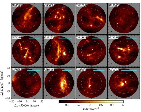
Data reduction was performed using CASA (version 4.7.134-DEV, r38011, for consistency with QA2 delivered products). Line-free continuum visibilities were created by flagging channels contaminated by spectral lines, where the input spectral windows were further visually inspected to check for emission at unexpected velocity ranges, partitioned out into a new measurement set with the split task, and channel averaged to to avoid bandwidth smearing. Together, this yields of dual polarization continuum bandwidth. The continuum image root mean square (RMS, ) is measured for each cleaned image within a region that excludes identified emission using the casaviewer tool. None of the images are dynamic range limited with peak image intensity divided by the RMS less than 200. We estimate the fiducial mass sensitivity given , thermally coupled gas and dust (), and OH5 dust opacity ). The methods for deriving dust mass values from the continuum emission are discussed in more detail in §4. The joint continuum was then iteratively cleaned with manual masking using the tclean task using the multiscale deconvolver and a robust weighting of 1, down to a brightness threshold of . An image cell size of was used for all continuum and spectral line maps. Self-calibration was not applied because the brightest sources in the image are only a few mJy, and not sufficiently bright such that a conservative self-cal produces a noticeable improvement without also increasing the image noise. The resultant images have a synthesized beam size of by ( angular diameter yields at ). The continuum images are shown in Figure 3.
2.2.2 ALMA spectral line reduction
The flexibility of the ALMA correlator enabled simultaneous observation of several molecular line transitions. Table 3 reports the details of the correlator configuration. We observed nine spectral windows (SPWs) with one wide-band, low-spectral resolution window centered at and eight high-spectral resolution windows centered on lines of interest. Table 4 reports the transition quantum numbers, rest frequencies, and upper energy levels (). The SPWs containing the \ceH2CO and \ceCH3OH transitions have a spectral resolution of and the other line SPWs have resolution. Line rest frequencies were taken from a combination of the SLAIM777http://splatalogue.net (F. J. Lovas, private communication, Remijan et al. 2007) and the CDMS (Müller et al., 2005) online spectroscopic databases. The line SPWs from the arrays were jointly imaged using the CASA task tclean with a Briggs robust parameter of , cell size of , and re-gridded to common spectral resolutions listed in Table 4. We find a typical RMS noise levels in the image cubes of (i.e., per channel or per channel) or when converted to brightness temperature units (HPBW beam size of ).
In this work we inspect the line image cubes for detection of emission, and for the presence of outflows traced by \ceCO and \ceSiO, but do not clean the data cubes. Due to the lack of full -coverage, the CO maps in particular show strong effects of spatial filtering near the systematic velocities that make the deconvolution process complex and error prone. Detailed analysis of the spectral line data is left to a future work. Table 6 lists the detection flags per target for the continuum, molecular lines, and outflows. Features are considered detections if they have peak intensities (“D”), weak detections if between (“W”), and non-detections if . Targets that exhibit bipolar outflows in CO or SiO are flagged “B” (discussed below in §3.2).
2.3 Image fidelity and MIR comparison
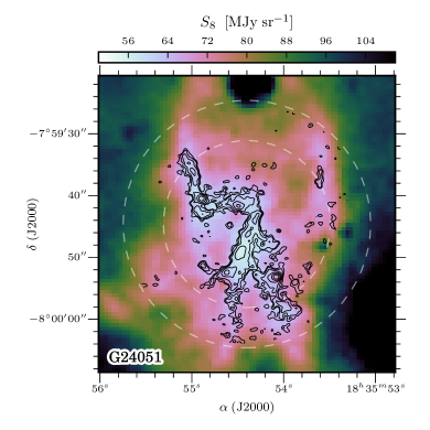
The dense gas features revealed in the continuum maps clearly show hierarchical structure, with bright ridges, filaments, and cores contained within larger, lower surface brightness features. Given the complexity within the maps and the systematic uncertainties of imaging, we compare the continuum images to an additional measure of gas column density at comparable resolution, MIR extinction. For appropriate configurations of distance and the MIR radiation field, clumps can appear associated with absorption features (EMAFs), where high column densities at close distances typically yield the strong MIR shadows that identify infrared dark clouds (IRDCs). MIR extinction mapping has the dual advantages of comparatively high-resolution, insensitivity to dust temperature, and lack of spatial filtering. We use the Spitzer GLIMPSE (Benjamin et al., 2003; Churchwell et al., 2009) IRAC Band 4 (, FWHM) mosaic to show the EMAF contrast. Figure 4 presents a map of the flux density with the ALMA continuum for source G24051 overlaid. The dense gas structures observed in the millimeter continuum show a remarkable consistency when compared with the column density features inferred from the of MIR contrast. This holds similarly true for the other clumps in the sample, as all show at least some MIR extinction. Qualitatively this good correspondence supports the fidelity of the emission structure detected in the ALMA maps.
2.4 Core identification and dendrogram
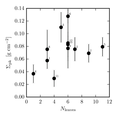
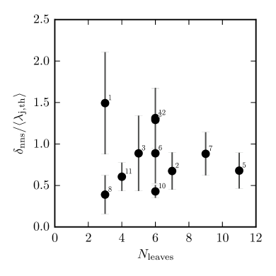
In order to analyze the fragmentation scale we first identify dense gas sub-structures using a segmentation algorithm. The nature of the tree data-structure in the dendrogram algorithm makes it well-suited to identifying and categorizing structure in images with hierarchical structure (see Rosolowsky et al., 2008), as opposed to a simpler segmentation algorithms, such as that done with a seeded watershed algorithm (e.g., clumpfind; Williams et al., 1994). We use the open source Python software library astrodendro to create the dendrogram and catalog of cores. The dendrogram has three principal tunable parameters, defining a minimum threshold value setting the floor or outer boundary of each tree, the minimum contrast or step size between nodes, and the minimum area . Because the noise varies considerably across the primary beam of each image, we apply the dendrogram to maps that have not been corrected for the weight of the primary beam. This effectively works to identify features with outer contours of constant statistical significance across the field of view, rather than outer contours of constant flux. Sources are extracted out to the limit of the maps, set to the 20% power point of the primary beam. We choose conservative values for each parameter, using , , and , applied to the unmasked images. Sources (i.e. leaves, or nodes without children) are then sub-selected to meet the criteria that the peak flux is . In total, we identify 67 sub-structures for the sample of 12 clumps. Figure 5 shows the dendrogram extracted dense gas sub-structures in each clump. Table 5 catalogs the measured positions, sizes, and flux densities of the sub-structures. We find an average number of sub-structures per clump of (median 6), with the maximum in G24051 and minimum in G23605. G23605 is the only clump with and is thus not included in the source nearest neighbor distance analysis. Figure 6 presents per clump versus , where a tentative increasing trend is observed, where clumps that have high are more fragmented than lower .
While in theory the distribution of integrated flux densities can be analyzed to measure a CMF, large observational uncertainties exist in practice that complicate its interpretation. The principal contributor arises from at least a factor of three uncertainty in ( uncertainty in ), due to uncertainty in the ISRF, local extinction, and uncertainty in the protostellar activity of each source. From single wavelength observations we do not have enough information to construct spectral energy distributions (SEDs) and measure average line-of-sight dust temperatures. Other significant systematics also arise from uncertainty in the missing flux density due to spatial filtering by the interferometer, dust opacity (), kinematic-derived heliocentric distance (), and the aperture or source boundary used to extract . For these reasons, we shall leave the study of the characteristic fragmentation mass and the CMF in SCCs to a future work utilizing complementary JVLA \ceNH3 observations that will provide both gas kinetic temperature and kinematic information (Svoboda et al. in prep.). The characteristic fragmentation length scale, on the other hand, can be inferred directly from the distribution of angular separations between sources with assumptions on how to correct for geometric projection.
3 Protostellar Activity
In this section we describe new evidence for protostellar activity, and in Sect. 5 we perform an analysis of the fragmentation scale from the sub-structure detected in the continuum. With the improved sensitivity and resolution of ALMA, multiple indicators of protostellar activity are observed for the first time. In particular bipolar molecular outflows detected in \ceCO and \ceSiO provide unambiguous evidence of embedded protostellar activity. The detection of molecular transitions with comparatively high upper excitation temperatures (-\ceCH3OH , ; p-\ceH2CO , ) and detection of bright, compact continuum emission (unresolved on scales smaller than ) are also suggestive of embedded, low- protostellar activity. Together, these data provide a clear indication of embedded protostars towards 11 out of 12 clumps.
3.1 Compact continuum sources
Numerous high SNR (signal-to-noise ratio, ), point-like sources are observed in the continuum images (Figure 3). We speculate such sources originate from the dense, centrally heated inner-envelopes of embedded protostars. In §4 we investigate whether the compact continuum sources are inconsistent with radiative transfer models of dense, starless cores.
We designate continuum sources as “compact“ if they are unresolved or are marginally resolved on the scale of the ALMA synthesized beam . Continuum sources are determined to be unresolved if a Gaussian fit to the image plane data using the CASA task imfit reports an deconvolved angular sizes . The deconvolved Gaussian FWHM are determined from subtracting the synthesized HPBW in quadrature from the fitted width, i.e. . These angular widths correspond to physical sizes of at heliocentric distances of . The brightest compact sources have typical peak flux densities between . All clumps aside from G28539 host a compact source with . Indeed, sources G23605 and G30120 host compact sources, even though they show limited fragmentation otherwise. While lacking extended continuum emission, the compact source G23605 S1 in has clear association with emission from multiple molecular species (\ceC^18O, \ceH2CO, \ceCH3OH) at the LSR velocity of the clump, determined from the \ceNH3 emission (, resolution; S16). G30120 S1 is a compact source near the eastern edge of the field with a strong \ceCO outflow and other molecular detections.
For comparison to nearby low-mass star forming regions, Enoch et al. (2011) carried out a survey of Class 0 YSOs in Serpens at with CARMA. The envelope masses range between (median ) and with integrated flux densities between (median ) and deconvolved size scales between (median ). With a heliocentric distance of to Serpens (Dzib et al., 2010), the median source flux density and size measured by Enoch et al. (2011) correspond to and when scaled to a fiducial distance of . If there are low- to intermediate-mass Class 0 YSOs with similar physical properties in these SCCs as in Serpens, then they would be consistent with the observed bright () unresolved point continuum sources. This is further supported by the frequent coincidence of outflows towards such sources, discussed in section §3.2. To determine whether the observed compact continuum sources are consistent with starless cores () embedded within the mapped clumps (), in §4 we compare a subset of the observations to radiative transfer models of starless cores.
Some continuum sources without molecular line detections may be background galaxies. Deep surveys performed with ALMA (Hatsukade et al., 2013; Carniani et al., 2015) have determined source counts of background galaxies at . The number of sources expected in the images with flux densities greater than over the 12 fields, measured as HPBW area for each pointing, outside of which the degraded sensitivity yields negligible background sources. This represents approximately of the detected sources, and thus does not have a significant effect on the calculation of the nearest neighbor separations or other estimated distributions of core properties.
3.2 CO & SiO Outflows
Ordered, bipolar molecular outflows driven by protostellar accretion provide a sensitive and unambiguous detection of embedded protostellar activity (see reviews by Arce et al., 2007; Frank et al., 2014). In this section we describe the properties of outflows detected with ALMA in \ceCO and \ceSiO .
Outflows are identified through visual inspection of the \ceCO datacubes in conjunction with the maps overplotted. While the emission structures in the \ceCO cubes are complex, bipolar outflows are clearly apparent as paired linear emission structures. These features are identified as linear features radiating from the same location with highly ordered red and blue velocity components that are detected over many velocity channels (, channels). Outflow candidate features with only a single red or blue component are also observed, but due to the greater ambiguity in identification these are not regarded as clear signatures of star formation activity. The \ceCO outflows are generally highly ordered in position and velocity, but spatial filtering of bright, extended emission and self-absorption near the source systemic velocity complicate the identification of low-velocity () outflow components. Higher velocity components of the spectra also suffer both self-absorption from foreground \ceCO clouds and confusion with bright Galactic emission, which can bias measurements of the maximum outflow velocity to lower values. Analysis of an example outflow in G24051 is presented in Appendix A.
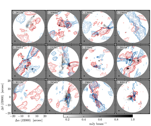
We find that 9 out of 12 clumps are associated with bipolar \ceCO outflows and 16 outflows in total are observed. We also find that 3 out of 12 clumps are associated with bipolar \ceSiO outflows and 4 outflows in total are observed. The clumps with outflows are reported in Table 6. Pairs of \ceCO outflows originating from the same continuum source are also observed, as seen in G23297 S2 and G29601 S1, which point to unresolved protostellar multiple systems. Figure 7 presents the ALMA joint array \ceCO integrated intensity maps for blue- and red-shifted velocity components.
We also detect \ceSiO emission towards several more continuum sources and positions without clear signs of ordered bipolar outflows. \ceSiO emission detection is a strong indicator of protostellar activity because of its origin in high-velocity shocks driven by protostellar outflows (Schilke et al., 1997). However, recent work has shown that low-velocity shocks () created by colliding flows may produce substantial distributed \ceSiO emission (Jiménez-Serra et al., 2010; Nguyen-Lu’o’ng et al., 2013; Louvet et al., 2016). Thus, considered by itself, a detection of relatively narrow linewidth () \ceSiO emission is not an unambiguous indicator of star formation activity. Maps of \ceSiO integrated intensities are presented in Appendix B.
3.3 G28539, a true starless clump?
The dark clump G28539 (upper-left corner of Fig. 3 & 7) shows no clear sign of \ceCO or \ceSiO outflows, and thus remains a starless clump candidate at the improved sensitivity of ALMA. Several indirect tracers of star formation are observed towards G28539 however and we discuss these in turn.
Moderately high-excitation molecular lines () are unlikely to be excited in the cold gas expected to be found in starless cores and quiescent clump gas. Detection of such lines in our observations are thus indirect evidence of embedded protostars, although as discussed in §3.2 it is possible some of these lines are excited from low-velocity shocks originating from colliding flows. In G28539, a compact source of weak emission \ceCH3OH and \ceH2CO is detected. These features are not coincident with continuum emission and may originate from non-protostellar shocks, shocks of undetected protostellar outflows, or of embedded protostellar cores that are below our detection limit. Similarly, a compact source of \ceSiO is also detected does not coincide with any continuum emission feature (it may be seen on the west side of the field in Fig. 15).
There exist weak sources in the vicinity of the clump boundaries as defined by the and emission, notably a faint source within the extinction feature east of the ALMA field (see panel in Fig. 1), a brighter source on the south-eastern outskirt of the clump, and a marginal feature coincident with the continuum source in the NW edge of the ALMA field of view. Because of the substantial contamination from evolved stars, emission alone is not a robust indicator of protostellar activity. If these sources are indeed protostars associated with the clump then they would be evidence that star formation has begun in G28539.
Deep radio continuum observations when available also provide a diagnostic of star formation activity because they are sensitive to the ionized gas in ultra- and hyper-compact Hii regions, ionized winds, and jets from low- to intermediate-mass protostars. Rosero et al. (2016) carried out deep Jansky Very Large Array (JVLA) C & K-band observations towards a sample of high-mass clumps which contains source G28539 in the field “G28.53–00.25”. The HPBW of the primary beam for the JVLA at C-band is at (LSB) and at (USB), with synthesized HPBW resolution of approximately in the A-configuration. Using the radio-continuum to bolometric luminosity scaling relations for protostars in Shirley et al. (2007) (Eq. 3), the measured sensitivity at can be converted to a bolometric luminosity sensitivity of , that is reasonably comparable to the PACS sensitivity from Hi-GAL. Here a faint point source is detected near the center of the ALMA pointing, detected in both side-bands at moderate significance (8 and in LSB, USB respectively). The measured in-band spectral index () favors a non-thermal synchrotron dominated source, but the weak constraint is consistent with thermal free-free emission at . The location (J2000) is not coincident with millimeter continuum or spectral line emission in the ALMA data. Given the lack of a clear association, we conclude that this radio continuum source is likely an extra-galactic contaminant and not an indicator of protostellar activity.
In summary, indirect evidence for star formation exists from two different tracers: (1) sources at the edge or outside of the ALMA field of view, and (2) ALMA detections of \ceCH3OH and \ceSiO that are not clearly associated with continuum sources. G28539 is the most massive clump in the sample () and shows fairly limited signs of fragmentation. After the ALMA observations G28539 is the only starless clump candidate remaining in our sample. It is thus a target of great interest for studying the initial conditions of high-mass star formation.
4 Modeling Continuum Sources
4.1 Starless core models
A diverse range of continuum sub-structures are found to be present in SCCs, from unresolved compact sources, filaments, to lower surface brightness extended emission. In this section we analyze whether cores with bright, unresolved continuum emission on scales () are necessarily protostellar even without detections of outflows or strong high-excitation molecular lines. We also model whether low- to intermediate-mass starless cores are accurately recovered in the observations and perform detailed modeling of high-mass starless core candidates in clump G28539.
To characterize the continuum features in our images we apply the radiative transfer code RADMC-3D (Dullemond et al., 2012) to self-consistently calculate the equilibrium dust temperature distributions of externally heated starless cores and to produce synthetic images. We follow a similar approach to modeling starless cores as found in Shirley et al. (2005) and Lippok et al. (2016). We apply conventional assumptions for the dust properties (Ossenkopf & Henning, 1994; Weingartner & Draine, 2001; Young & Evans, 2005) and interstellar radiation field (ISRF, Draine, 1978; Black, 1994). A detailed description of the computed models may be found in Appendix C.
We apply a spherically symmetric Plummer-like function to parametrize the model radial density profile (Plummer, 1911; Whitworth & Ward-Thompson, 2001; Lippok et al., 2016). The gas density profile can be expressed as:
| (1) |
for radius , inner gas density , outer gas density , flat radius , and power law exponent (n.b. an isothermal Bonnor-Ebert sphere may be approximate with ; Ebert, 1955; Bonnor, 1956). The strength of the interstellar radiation field (ISRF) is varied from the local value by a multiplicative scale factor . We compute models, randomly sampling the parameter space by drawing values from a uniform distribution in log-space within the ranges for the parameters , , , and , while is drawn uniformly in linear space. Models are evaluated on a logarithmic radial grid from to . These values are chosen to cover the range of values from the sample of low- and intermediate mass cores in Lippok et al. (2016) but extended to higher and smaller . After computing the radiative transfer, the models are ray-traced by RADMC-3D and projected to a fiducial distance of .
4.2 Model recovery
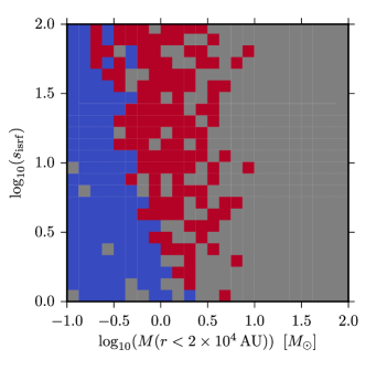
We find that of the computed models () meet the detection threshold of when convolved with a Gaussian beam. The cut in peak flux density has no effect on the recovered distributions of and , and minimal effects on and , with an increase in the median values by a factor of and , respectively, over the distribution of model cores.
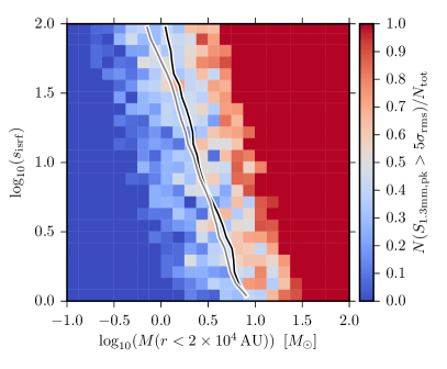
It is important to keep in mind that the suite of model cores is constructed to span the parameter space of relevant values, not to represent an observed or predicted core mass function. We do not use the fractions of detectable cores to infer completeness, but to show the expected range of physical parameters for which cores can be recovered. To estimate this, we sort the models by and , counting both the fraction of detectable cores, and regions of parameter space with at least one detectable model (Fig. 8). Computing the detection fraction in this way has the effect of marginalizing over our uncertainty in , , , and , that are poorly constrained with our single wavelength maps. Figure 8 (left) shows that at 50% completeness, the cores at are recovered for , and that this extends down to for the extreme value . Figure 8 (right) shows that it is possible however to recover lower-mass cores if the ranges of models is restricted to those that are the most compact (where , ) and have high central densities (). For these compact sources, models may be recovered at and down to for .
From these models we can infer that the completeness expected from our point-source sensitivity, at , is an underestimate if the majority of cores are resolved (see also Appendix A in Beuther et al., 2018). Low-mass cores with extended profiles will thus go undetected with a criteria based on peak intensity, leading to our seemingly shallow limit of . Observationally, we must approach extended emission at low-SNR with caution because there is extended structure in the maps on scales larger than the primary beam that cannot be adequately cleaned. For this reason we do not attempt to identify or catalog sources down to the limits of statistical significance for extended and spatially-integrated flux densities but maintain a conservative detection limit based on source peak flux density. The typical integrated flux density of a source is ( assuming and ), and generally consistent with the thermal Jeans mass for a uniform medium at the density of the clump, where for thermal Jeans length and average density (McKee & Ostriker 2007; see §5 for an analysis of the Jeans length ).
4.3 Synthetic observations with CASA
We now investigate whether the models of starless cores provide adequate fits to the brightness profiles present in the SCCs of this survey. We find that compact sources of continuum emission that are unresolved (i.e. deconvolved sizes , ) are poorly fit by models of starless cores. Without multiple wavelength observations or gas kinetic temperature information, the radial dust temperature profiles of the cores are poorly constrained. Because of the substantial systematic uncertainties presented in single wavelength observations and potentially undetected embedded protostars, we do not perform a fit to every continuum source, but select a few characteristic examples for quantitative comparison. We create synthetic observations from the models using the CASA sm module by predicting onto the observed visibilities (gridded beforehand for computational efficiency) and imaged without noise using the same tclean configuration as the observations. This does not introduce a significant effect on the models however because nearly all the flux is concentrated on radii or angular diameters of , appreciably less than half of the array HPBW, and substantially less than the maximum recoverable scale of from the array. A subset of models were further tested for consistency, because the aim of this comparison is for an understanding of a few representative sources and not detailed parameter estimation, we do not image the full suite of models; rather, we convolve the models with the angular size of the synthesized beam () and convert to radial brightness profiles.
4.4 Comparison to observations
We compare the observations and models using a method based on the -statistic, where the reduced may be expressed as
| (2) |
for degrees of freedom , independent measurements , measurements , model values , and variances . We discriminate between models based on the goodness of fit metric from Robitaille et al. (2007) and Robitaille (2017). Robitaille et al. apply the heuristic that models with are considered good fits and rejected as poor fits otherwise. Robitaille et al. further note that the Bayesian likelihood under the assumption of normal errors (i.e., for data , parameters , and model ) yields too stringent a definition of probability given systematic sources of error in the measurements and poor physical correspondence of the model to nature. This ultimately provides a more conservative criteria for rejecting poor fits as the heuristic likely overestimates uncertainties.
We consider two example starless core candidates, G28539 S2 and S4 (see Fig. 5 and Table 5, because they (1) lack unresolved continuum emission at their center, (2) host no outflows or other indicators of star formation activity, and (3) are relatively isolated such that radial brightness profiles can be adequately extracted. G28539 S2 and S4 are also of interest because they are among the brightest such sources, and thus are good high-mass starless core candidates.
We extract radial brightness profiles for the cores by extracting the integrated flux density within diameter annuli about the central position. Uncertainties in the integrated flux densities are calculated as the for the solid angle of the annulus and the synthesized beam solid angle . The radial brightness profiles of the models are then compared by Equation 2 for degrees of freedom (maximum radius ). Well-fit models are then selected where . Figure 9 shows the best fit models compared to the observations, and Figure 10 shows the radial brightness profiles with the range of fits. We find that the extended brightness profiles are well fit by the starless core models ( and for S2 and S4 respectively). If the range of models are limited to those that resulted in in order to be broadly consistent with the clump-average temperature derived from the Hi-GAL SED and GBT \ceNH3 fits (see also the detailed considerations in Tan et al., 2013), then and , for the median, maximum, and minimum model mass. With a core star-formation efficiency of it is possible that these cores may form high-mass stars (). Assuming a formation efficiency from models regulated by outflows (Zhang et al., 2014) the maximum expected stellar mass for S2 could be . Given the fact that these cores are not associated with outflows in the ALMA data or other high-excitation molecular lines, they are excellent candidates for high-mass starless cores.
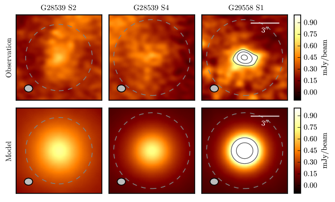
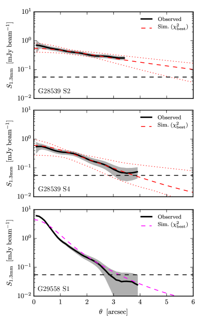
G29558 S1 represents the class of compact continuum sources in our data set. Analysis of this source is then a test of whether the compact sources are well described by starless core models, or alternatively, likely to host embedded protostars. This continuum source has some surrounding extended continuum emission, does not show clear outflows traced by \ceCO or \ceSiO, but is associated with weak \ceCH3OH and p-\ceH2CO emission. It is bright with peak flux density and is similar to other continuum sources with associated outflows. We find that the models poorly fit the observations, with and no models for . The properties are pushed to the extremes of parameter space: , , and . The moderate is a compromise between the compact and extended components of the brightness profile. The poor model fits to G29558 S1 do not strictly require that it or any other individual source is protostellar (models with and would likely fit the observations). However, such extreme starless cores are unlikely to be observed in significant numbers in our sample, where of fragments are compact continuum sources. The free-fall timescale of a core with would be , and for would be . These are shorter than the inferred ages from the extent and velocity of the observed outflows, although these have substantial uncertainties. Together, the observed properties of these compact continuum sources are more favorably explained as embedded low- to intermediate-mass YSOs, which at would be both of comparable brightness and unresolved (see §3.1). A detailed analysis of the starless and protostellar core properties and dynamics will follow in a future work incorporating \ceNH3 data from the VLA observations.
5 Fragmentation Scale
5.1 Nearest neighbor separations and Monte Carlo simulations
We characterize the linear fragmentation scale in terms of the nearest neighbor separation between dendrogram leaves in each clump. Geometric projection of sources in the plane of the sky will systematically decrease from the true value, . In this work we employ Monte Carlo random sampling to de-project statistically. Thus while the uncertainty in may make constraints for any individual pair of sources quite weak, with prior assumptions on the relative positions of sources, the posterior distribution from the ensemble of all measurements in our sample of SCCs can be readily constrained.
Monte Carlo sampling is used to draw realizations of relative line-of-sight distances , computing for each source from the Cartesian coordinates . We use the hierarchical classification of sources in the dendrogram to discriminate between two methods of drawing values: (i) isolated sources and (ii) sources with common surrounding emission. If sources are isolated (Case i), forming a tree with a single branch, then for each trial we draw line-of-sight distances from a Gaussian distribution with standard deviation (FWHM ), chosen such that the double-sided interval is , which is the approximate diameter inferred from the maps (cf. Fig. 1 & 4). If sources are associated within the same branch of the dendrogram (Case ii; ie. they are within a common base iso-contour of emission) then we assume that those sources are connected in a filamentary gas structure with unknown inclination with respect to the observer. For each trial, we draw a common inclination for the group, pivoting along the major axis, with the pivot axis fixed to at the projected geometric center. Inclinations are drawn such that the length between the two components with the maximum separation is less than , thus where is drawn uniformly within the interval . If , then is drawn uniformly within , such that to extend out to a typical clump effective radius of . In total there are (26%) isolated sources and (74%) grouped sources. Without more detailed knowledge available, informed from either additional observational data or theoretical simulations, we consider this scheme a conservative way to correct the data for geometric projection. While the assumptions in the correction are simple and imperfect, for brevity we refer to the distributions of MC trials as “projection-corrected” below to distinguish it from the projected data. Extensions of this method may opt to use more sophisticated schemes to group sources beyond common millimeter continuum emission, such as grouping sources through a lower density kinematic tracer or a source-density based clustering algorithm.
With no correction applied, the distribution of projected separations has a median value of with percentile interval of . To calculate the projection-corrected separations, we compute ealizations for each clump, and find with and a percentile interval of . For comparison, if we assume that all sources are uniformly distributed within a spherical volume of radius the following projection correction may be applied:
| (3) |
as is done in Myers (2017). If we assume from the radius of the 20%-power point of the ALMA primary beam at , then this correction factor would be and , which is larger than the median value computed above from the MC trials by .
5.2 Jeans length comparison
To consistently compare values between clumps with different physical conditions, we scale the values by the clump average thermal Jeans length, the minimum wavelength for gravitational fragmentation in an isothermal, uniform medium. The thermal Jeans length can be expressed as (McKee & Ostriker, 2007):
| (4) |
where is the isothermal sound speed ( for ), is the gravitational constant, and is the average volume density. For the accurate propagation of uncertainties in the calculation of , we perform MC random sampling of the relevant observational uncertainties in from the dust mass surface density () and heliocentric distance. The total (i.e., gas) mass surface density are calculated with
| (5) |
for source integrated flux density , source solid angle , Planck function evaluated at dust temperature , opacity per mass of dust Ossenkopf & Henning (1994), mean molecular weight , and dust-to-gas mass ratio (values are further described in Appendix C).
The fragmentation measured within the ALMA maps is most sensitive within the HPBW () of the primary beam, so an estimate of within this volume we consider to be the most representative density for the computation of . Clump average densities on angular scales () larger than the HPBW likely underestimate . Likewise, image-integrated flux densities from the array data possibly underestimate the from spatial filtering. Due to the unfavorable match in resolution compared to the Hi-GAL () or BGPS (), we extract flux densities from the ATLASGAL maps () at the position of the ALMA pointing for each clump within a beam-sized diameter circular aperture to measure . Use of the single millimeter flux mitigates one systematic uncertainty in choosing between Hi-GAL SED fits with or without the band included, or using Hi-GAL SED fits that are over the emission for the full clump rather than the peak at consistent angular resolution. The clump average dust temperatures from SED fits to the Hi-GAL data range from , but some systematic uncertainty exists with averaging over larger volumes than the ALMA field of view and choices in including the band. We choose a conservative dust temperature distribution by assuming a Gaussian dust temperature distribution ( interval). For consistency this temperature is also used for the gas kinetic temperature in . We propagate the uncertainty in heliocentric distance based on the distance probability density function (DPDF) from Ellsworth-Bowers et al. (2015) for each clump. All sources are well-resolved to the near kinematic distance, and have a fractional uncertainty. We sample the distributions for , , and for each MC trial of in the calculation of to combine with a trial of to compute the quotient for each clump. The computed median volume densities for the clumps in the sample range between and with associated values of the thermal Jeans length between (). The median of samples from all clumps is (). No correlation is observed between and the number of cores/leaves in each clump (Fig. 11).
Probability density functions (PDFs) of are computed for each clump by performing Monte Carlo random sampling of the observational uncertainties in as described above and sampling the de-projected source separations (see §5.1). Figure 12 (left) shows the distributions of for each clump sorted in descending order by the number of continuum sources. The separation distributions show a bi-modal tendency with peaks at and , and with long-tails extending to high values . The distinct peaks at small values of (all well-resolved) likely result from closely spaced, connected sources where is not strongly effected from sampling the inclination distribution. Median values of the distributions range between . The values are generally consistent with the thermal Jeans length, but the high frequency of sources with sub-Jeans separations may indicate hierarchical fragmentation at multiple scales. With the initial fragmentation on the clump scale, a further fragmentation on the “core scale” would proceed on sizes and densities . If such hierarchical fragmentation proceeds principally with two resultant fragments on the core scale, then the second nearest neighbor distance would measure the above level in the hierarchy and recover the spacing of the clump scale. This is supported by a plot of the second nearest neighbor distance distributions, shown in Figure 12 (right), that shows clumps with more uni-modal distributions, with modes and median values at or slightly above the thermal Jeans length. Median values of the distributions are greater than those for but generally fall within a similar range between .
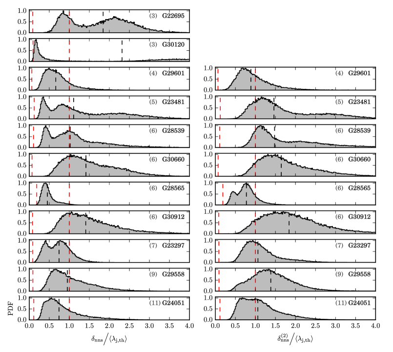
We compute PDFs for each clump (see above) and the ensemble distribution composed of all separation measurements from each clump aggregated together (Fig. 13). The ensemble separation distribution is used to define a representative fragmentation scale from the SCCs in this survey. As these clumps are at similar distances and blindly selected from Galactic Plane dust continuum surveys, the measured ensemble sample properties may be used to cautiously infer the properties of the Galactic high-mass SCC population (). Additional observations are required to directly constrain the properties of SCCs with (if they exist outside of the Central Molecular Zone) or SCCs below the mass range of this sample, . Figure 13 shows the cumulative distribution function (CDF) for the ensemble of measurements as drawn from the MC sampling for the projected separations, projection-corrected separations, and relevant scales such as the resolution and primary beam HPBW. The projection-corrected ensemble distribution has a median value of with a percentile interval of . The percentiles for , , , and are, respectively, , , , and . Overall, the sample of SCCs show a fragmentation scale that is well characterized by the thermal Jeans length.
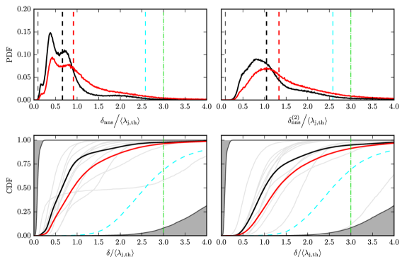
The inner and outer grey areas show the scaled synthesized beam () and scaled -point of the primary beam (). The scaled HPBW () of the primary is also shown (dashed cyan). Upper left: PDFs of different length scales , with the same color coding. The dashed lines show the values of the 50th percentiles. Lower right: CDF for the second nearest neighbor separations, . Upper right: PDF for the second nearest neighbor separations, .
A relatively small fraction of the separation distribution is inconsistent with the thermal Jeans length, for . The large separations do not result from a single or small number of clumps with consistently large separations, but from isolated individual sources within clumps that show fragmentation near the thermal Jeans length. G30660 and G30912, for example, have a significant proportion of the distribution at large separations (see Fig. 12 left), but do not have peculiar dust temperatures, between from Hi-GAL SED fits. This portion of the separation distribution may indicate an additional scale for hierarchical fragmentation where a source of non-thermal support prevents fragmentation at the thermal Jeans scale.
The Jeans length can further take into account sources of non-thermal support, such as turbulence or magnetic fields, by using an effective sound speed
| (6) |
through the contribution of a non-thermal velocity dispersion . From S16, 9 out of 12 clumps have measured from \ceNH3 (at resolution). The measured velocity dispersions (i.e. ) determined from the spectral line model fit range between with a median value of , corresponding to for at (where ). Replacing with in Equation 4 yields the effective Jeans length, or when turbulence is the dominant source of non-thermal support, the turbulent Jeans length . Because , the increase (median ) yields a similar scaling for . In comparison, () occurs at the percentile, and thus while such separations are not absent from the data, they are also not representative of the fragmentation measured within the ALMA maps. The length scale distribution is incomplete beyond , where of the MC trials would have 3D separations greater than or equal to the FOV ().
6 Discussion
The physical processes regulating fragmentation in molecular clouds remain an open problem in star formation. How much are SCCs supported against gravitationally induced fragmentation from non-thermal forms of pressure, such as magnetic fields (-fields) and/or turbulence? Individual SCCs have been studied at high-resolution (Beuther et al., 2015b; Sanhueza et al., 2017), but we shall discuss a systematic set of observations on a representative sample of high-mass SCCs. Here we describe the fragmentation characteristics of SCCs in the context of theoretical models of star and cluster formation and compare to existing high-resolution observations of clumps and IRDCs.
6.1 Cylindrical Fragmentation in SCCs
As shown in §5, we find that clumps fragment at scales consistent with the thermal Jeans length in SCCs. It is known however that geometry and non-thermal support affect the predicted fragmentation scale, producing deviations from that expected for an isothermal, uniform medium. In this section we discuss how the fragmentation scale observed with ALMA compares to different characteristic length scales.
Filaments are ubiquitous in both observed molecular clouds and simulations (e.g., Barnard, 1907; André et al., 2014; Smith et al., 2016), and thus cylindrical geometry is of special significance to dense molecular regions. On larger spatial scales observable in MIR extinction, it is clear that the clump peaks are embedded in filamentary gas structures (see Fig. 1 and G23297 for a good example). An infinite, self-gravitating cylinder is unstable to axisymmetric perturbations or “sausage” instability, where the cylinder fragments at the scale of the fastest growing mode of the fluid instability (Chandrasekhar & Fermi, 1953; Ostriker, 1964; Larson, 1985; Nagasawa, 1987; Inutsuka & Miyama, 1992). For a pressure confined isothermal gas cylinder of radius and scale height (where is the central density of the cylinder) then the fastest growing mode depends on the ratio of and (Nagasawa, 1987). In the case where then ; and, alternatively where , then (Nagasawa, 1987; Jackson et al., 2010).
Is the isothermal, cylindrical fragmentation scale representative in SCCs? The approximation of SCCs as isothermal is imperfect due to shielding that decreases the temperatures of inner regions, but the assumption is generally more valid than clumps with active HMSF and substantial internal protostellar heating and feedback. Observed aspect ratios of over the full clump extent support the approximation of an infinite cylindrical geometry. The typical radial extent of the SCCs as observed in the MIR extinction maps suggests . Assuming that the cylinder central density is equal to the observed clump peak density (i.e. ) then , and thus roughly satisfies the condition . Note that for equal to the clump peak density then this simplifies to , or for the median , . We find that is not representative of the distribution in SCCs, with the observed .
Observational studies carried out on larger spatial scales than this work support as a characteristic scale in filaments (Beuther et al., 2015a; Friesen et al., 2016). While these studies did not have sufficient spatial resolution to adequately resolve the thermal Jeans length, they probe separations on the clump scale and larger than , as observed with ALMA. This work complements the larger-scale studies by identifying fragmentation on the clump Jeans length at an early evolutionary phase. This is supported by the results of Kainulainen et al. (2013) who with Spitzer MIR extinction mapping find that the molecular filament G11.11–0.12 is well described by filament fragmentation and turbulent on and on smaller scales. Beuther et al. (2015a) in an analysis of the fragmentation in the star-forming filament IRDC 18223 find a mean fragment separation of , consistent with a thermal of the filament, approximately twice that of , however the authors note that measures of should be considered an upper limit due to the sensitivity and resolution of the data. Friesen et al. (2016) in a survey of the entire Serpens South molecular cloud (as part of the GBT Ammonia Survey, GAS; Friesen et al., 2017) find that the nearest neighbor separations of dense gas structures within the same filament are significantly larger than and are well represented by . The spatial resolution is limited however to approximately , and thus does not properly resolve in sources with . The above surveys support the view of hierarchical fragmentation by gravitationally unstable filaments, but lack the resolution to test what fragmentation process dominates on the scales of individual cores embedded within the clumps. The measurements of the fragmentation scale presented in §5 complement the above studies at resolutions down to and provide further support to the view that filaments initially fragment at and then further fragment at .
6.2 Comparison to more active regions
Direct observations of star-forming IRDCs and embedded protoclusters have found fragmentation consistent with the thermal Jeans length (Palau et al., 2015; Beuther et al., 2015b; Teixeira et al., 2016; Busquet et al., 2016; Beuther et al., 2018) but it is unknown if these systems represent the initial state of fragmentation. Because high-mass SCCs may represent an initial stage of protocluster evolution before the formation of a high-mass star, they offer unique insight into the physical processes regulating fragmentation when compared to more evolved systems. From a survey of dense star-forming cores Palau et al. (2015) find that the fragmentation on scales is best explained through thermal fragmentation. Similar results are found at sub-core spatial scales of towards the Orion Molecular Cloud 1S (OMC-1S; Palau et al., 2017) and also consistent with the fragmentation measured in OMC-1N (Teixeira et al., 2016). While the measured median nearest neighbor separation in SCCs is consistent with the thermal Jeans length of the clump gas, the distribution also shows a distinct peak at approximately an order of magnitude higher gas density near (see Figs. 12 & 13). These results may indicate continued thermal Jeans fragmentation such as in OMC-1S and OMC-1N. Beuther et al. (2015b) find results approximately consistent with thermal Jeans fragmentation towards the IRDC 18310–4, and while showing faint emission, has similar physical properties to the SCCs in this sample. Similarly an analysis of the star-forming IRDC G14.225–0.506 favors thermal Jeans fragmentation (Busquet et al., 2016). Beuther et al. (2018) present a minimal spanning tree analysis of the separations in the CORE survey of 20 luminous () high-mass star forming regions and find fragmentation at scales on the order of the thermal Jeans length or smaller. As a possible explanation for the sub-Jeans length scales, Beuther et al. (2018) suggest that bulk motions from ongoing global collapse may have brought the fragments within closer proximity after having initially fragmented on the thermal Jeans scale. All of the sources in the CORE survey are high-mass protostellar objects (HMPOs) and more evolved than this sample. Thus our finding of fragmentation on the thermal Jeans length at an earlier evolutionary stage supports the interpretation of the COREs results and conclusion that the measured fragmentation scale may be impacted by the dynamical evolution of the protocluster.
The agreement between the nearest neighbor separations and the thermal Jeans length appears to favor a Jeans fragmentation process for stellar cluster formation. Indeed the thermal Jeans mass in typical star forming clumps is approximately , which corresponds well with the stellar mass at the peak of the Initial Mass Function. Therefore, Larson (2005) argued that the thermal Jeans process is responsible for the formation of lower mass stars in a cluster. Zhang et al. (2009) found that cores forming massive stars often , an order of magnitude greater than the thermal Jeans mass of its parental clump. These cores require additional support from turbulence to account for their formation. Furthermore, the observed measurements imply that thermal physics provide the dominant form of support, but additional models exist to describe the thermal fragmentation process that differ in geometry and density profile. For example, Myers (2017) present 2D axisymmetric models of filamentary structure that fragment through the thermal instability of Bonnor-Ebert spheres above a threshold minimum density. Because the Bonnor-Ebert radius and Jeans length have the same dependence on temperature and density with only slight differences in numerical coefficients, this leads to a fragmentation approximately equal to . When compared to the observed median from §5, the spacings between cores predicted by Myers (2017) is (for a concentration factor ) are broadly consistent.
6.3 Coeval formation of low- and high-mass protostars?
It is not clear if SCCs are the progenitor environments of high-mass star formation. Their high total masses (), high central densities (), cold gas kinetic temperatures (), and low virial parameters () (Wienen et al., 2012; Svoboda et al., 2016) all point to persistent, bound clumps with the likely necessary physical conditions for high-mass star formation (McKee & Ostriker, 2007). However, no high-mass protostars are observed. These observational facts are consistent with a scenario where high-mass stars form in SCCs through thermal fragmentation, and then accrete clump gas as initially low-mass protostars. Thus, SCCs may represent a very early and unique stage in protocluster evolution preceding the formation of high-mass protostars. This view is supported by cluster-scale theoretical simulations that incorporate protostellar and stellar feedback (Smith et al., 2009; Wang et al., 2010; Peters et al., 2010a, b, 2011). Smith et al. (2009) find that no high-mass starless cores are formed in their models, and that massive stars originate from low-to-intermediate mass cores that become high-mass protostars via accretion. The mass accreted comes primarily from the surrounding clump at scales (Smith et al., 2009; Wang et al., 2010).
Cyganowski et al. (2017) in a study towards the deeply embedded protocluster G11.92–0.61 discover low-mass cores in the accretion reservoir of the accreting high-mass protostellar object “MM1” with mass (Ilee et al., 2016). The detection of coeval low- and high-mass protostars is consistent with competitive accretion-type models of star formation (see §1). At a comparable distance of kpc (derived from maser parallax Sato et al., 2014) and total mass to the SCCs in this study, G11.92-0.61 is more evolved, coincident with several indicators of high-mass star formation, such as Class I & II \ceCH3OH masers, \ceH2O masers, a GLIMPSE Extended Green Object (Cyganowski et al., 2008), numerous “hot core” molecular lines, and high-velocity collimated outflows. The sample of SCCs in this study complement the study of G11.92–0.61 in Cyganowski et al. (2017) through ALMA observations at similar resolution and sensitivity for clumps in a less active evolutionary state. In contrast, we find no clear high-mass protostellar cores or high-mass protostars in our sample of SCCs, while numerous accreting low-mass protostars are observed, as evidenced by bipolar outflows in \ceCO/\ceSiO. If a few of the protostars in SCCs will accrete up to high-mass stars, for which the accretion reservoir of the clump is sufficient, then these observations support a coeval mode of protocluster formation at earlier phases. When initially only low- to intermediate-mass protostars are present, this coeval formation may also be termed “low-mass first” to lie in contrast to the monolithic collapse of turbulently supported high-mass cores. The competitive accretion-type simulations performed by Smith et al. (2009) find that high-mass stars form initially from intermediate mass pre-stellar cores near the center of the gravitational potential which accrete principally from collapsing clump gas up to high-mass condensations. An important feature of the Smith et al. (2009) model is that low-mass protostars form within the accretion reservoir of the central protostar, at separations . This is well matched to the distribution of nearest neighbor separations found in this work of (see §5). As Smith et al. (2009) point out, this signature is likely the most detectable at the early evolutionary phases of the clump where sources are less centrally concentrated in the potential and bright sources of emission are not present.
In contrast to the results of Cyganowski et al. (2017), Zhang et al. (2015) in a study of the protocluster G28.24+0.06 P1 failed to detect a distributed population of low-mass cores with Cycle 0 ALMA observations. Based on this Zhang et al. (2015) draw the conclusion that the distributed population of low-mass cores forms at a later evolutionary stage and that they are not, at least for the initial generation of protostars, coeval. Because G11.91–0.61 is at a later evolutionary stage, the distributed population of low-mass protostars observed in it may have developed after the massive cores formed. The SCCs in this study are in a similar early evolutionary phase as G28.24+0.06 and also similarly lack high-mass protostars (the maximum core mass in G28.4+0.06 is ). Accurate core masses are required for a quantitative analysis of the mass segregation and related length scales, but the diversity in morphologies shown within the sample, from distributed (e.g. G30660, G29558) to weakly fragmented (e.g. G28539, G29601), supports the presence of a distributed low-mass core population at the initial evolutionary phase for some systems. It is possible that depending on the initial level of support provided against fragmentation individual systems develop with varying degrees of hierarchy and segregation, and that the conclusions of Zhang et al. (2015) and Cyganowski et al. (2017) may both be correct for sources of different initial physical conditions.
The short evolutionary timescales of high-mass starless clumps, for S16, is also consistent with the simulations of Smith et al. (2009) that show that the central, resultant high-mass protostar accretes in the clump dynamical time, over a diameter of (equivalent to the ALMA HPBW) (see also Wang et al., 2010). Similarly, (Battersby et al., 2017) perform a lifetime analysis of dense, molecular gas () analyzed on a per-pixel basis from a Hi-GAL field near . They find a timescale that is consistent for starless regions of , although with substantial uncertainty. The similarity in timescales is reasonable, as once a high-mass protostar forms, it would be accompanied by observational star formation indicators that identify it as a protostellar clump and remove it from the SCC category, as determined in S16. Further, we also observe hierarchical fragmentation as evidenced by the multi-modal distribution of nearest neighbor separations (see Fig. 13), as seen in G11.92–0.61. The ubiquity of filamentary structures observed (see Fig. 3) may also point to accretion mediated by sub-sonically gravitationally contracting filaments (Smith et al., 2016). This may suggest that while self-gravitating, turbulent clumps are not globally collapsing, accretion may yet be mediated through locally collapsing filaments. This latter point will be the topic of further research investigated with ALMA observations of to study the kinematics of the filaments observed in this sample SCCs.
7 Conclusions
We present the first systematic observations of a large sample of well-vetted starless clump candidates with ALMA at high-resolution () capable of resolving the thermal Jeans length and sensitivity () sufficient for detecting point sources down to and moderately compact starless cores down to ). The targets are selected from a complete sample of clumps identified from large Galactic Plane surveys. The sample is composed of 12 high-mass SCCs within from Svoboda et al. (2016) and Traficante et al. (2015) which did not show detected emission at or other star formation indicators. Because these systems have not been affected by the extreme (proto-)stellar feedback of high-mass stars they are ideal environments to study the initial conditions of protocluster evolution. Our main findings are:
-
1.
The newly sensitive ALMA Band 6 () data show multiple indicators of low-/intermediate-mass star formation activity present in 11 out of 12 formerly starless clump candidates. This is determined through the presence of bipolar outflows detected in \ceCO and \ceSiO emission, and high-excitation p-\ceH2CO emission (). These observations caution the interpretation of infrared dark clouds and SCCs identified from Galactic Plane surveys as quiescent, and unless shown otherwise are, given the findings towards this sample, likely to host low-/intermediate-mass star formation activity below the luminosity completeness of current surveys.
-
2.
We compare representative examples of resolved and unresolved continuum sources with radiative transfer models of starless cores computed with RADMC-3D . Unresolved sources are poorly fit by starless core models with typical physical properties. The range of models does not encompass the most compact and dense cores (, ), but the short core free-fall times () and the observed similar flux-density to Gould’s Belt low-/intermediate-mass protostars, support the conclusion that these cores are protostellar even without identified outflows in \ceCO or \ceSiO.
-
3.
Two high-mass starless core candidates in G28539 are identified and well fit by starless core models, with and . Without supplementary measurements to infer the dust temperature profile, the masses are highly uncertain, and are consistent within the uncertainties of only forming an intermediate mass star ().
-
4.
G28539 is the sole remaining starless clump candidate without any definitive indications of protostellar activity from the ALMA observations. It is the most massive SCC in the sample (, ), and stands as an excellent target to study the initial conditions of protocluster evolution. A marginal source, however, is observed coincident with continuum source (G28539 S1) near the NW edge of the ALMA field, which may be evidence or protostellar activity. Further indirect evidence for star formation exists from compact \ceSiO and \ceCH3OH emission, although the source of emission is not associated with a continuum source. If these signatures are indeed associated with protostellar activity there would be no true high-mass starless clumps in this sample.
-
5.
A high degree of fragmentation is observed, with nearest neighbor separations consistent with the clump scale thermal Jeans length (). In context of previous observations that on larger scales see separations consistent with the turbulent Jeans length or cylindrical thermal Jeans length, our findings support a hierarchical fragmentation process, where the highest density regions of SCCs are not strongly supported against fragmentation by turbulence or magnetic fields.
-
6.
Observed embedded low- to intermediate-mass star formation and thermal Jeans fragmentation in high-mass SCCs are consistent with models of star formation that form high-mass stars through gravitationally driven cloud inflow, in which low- and high-mass stars form coevally. However, further observations and followup study are necessary to properly characterize the clump star formation efficiency, protostellar accretion rates, and presence of dynamical flows in molecular tracers to validate this conclusion.
8 Acknowledgments
We are grateful to the anonymous referee for many helpful comments and suggestions. BES would like to thank Al Wootten and the staff of the NRAO North American ALMA Science Center, Kimberly Ward-Duong for helpful discussions, and Viviana Rosero for access to the JVLA C Band image towards G28539. BES was supported in part by the NSF Graduate Research Fellowship under grant No. DGE-114395. YLS and BES acknowledge the support from the NSF AAG grant No. AST-1410190. HB acknowledges support from the European Research Council under the European Community’s Horizon 2020 framework program (2014–2020) via the ERC Consolidator Grant “From Cloud to Star Formation (CSF)” (project number 648505).
References
- Aguirre et al. (2011) Aguirre, J. E., Ginsburg, A. G., Dunham, M. K., et al. 2011, ApJS, 192, 4, doi: 10.1088/0067-0049/192/1/4
- André et al. (2014) André, P., Di Francesco, J., Ward-Thompson, D., et al. 2014, Protostars and Planets VI, 27, doi: 10.2458/azu_uapress_9780816531240-ch002
- Arce et al. (2007) Arce, H. G., Shepherd, D., Gueth, F., et al. 2007, Protostars and Planets V, 245
- Barnard (1907) Barnard, E. E. 1907, ApJ, 25, doi: 10.1086/141434
- Battersby et al. (2010) Battersby, C., Bally, J., Jackson, J. M., et al. 2010, ApJ, 721, 222, doi: 10.1088/0004-637X/721/1/222
- Battersby et al. (2017) Battersby, C., Bally, J., & Svoboda, B. 2017, ApJ, 835, 263, doi: 10.3847/1538-4357/835/2/263
- Benjamin et al. (2003) Benjamin, R. A., Churchwell, E., Babler, B. L., et al. 2003, PASP, 115, 953, doi: 10.1086/376696
- Bergin & Tafalla (2007) Bergin, E. A., & Tafalla, M. 2007, ARA&A, 45, 339, doi: 10.1146/annurev.astro.45.071206.100404
- Beuther et al. (2007) Beuther, H., Churchwell, E. B., McKee, C. F., & Tan, J. C. 2007, Protostars and Planets V, 165
- Beuther et al. (2015a) Beuther, H., Ragan, S. E., Johnston, K., et al. 2015a, A&A, 584, A67, doi: 10.1051/0004-6361/201527108
- Beuther et al. (2015b) Beuther, H., Henning, T., Linz, H., et al. 2015b, A&A, 581, A119, doi: 10.1051/0004-6361/201526759
- Beuther et al. (2018) Beuther, H., Mottram, J. C., Ahmadi, A., et al. 2018, ArXiv e-prints. https://arxiv.org/abs/1805.01191
- Black (1994) Black, J. H. 1994, in Astronomical Society of the Pacific Conference Series, Vol. 58, The First Symposium on the Infrared Cirrus and Diffuse Interstellar Clouds, ed. R. M. Cutri & W. B. Latter, 355
- Bonnell et al. (2001) Bonnell, I. A., Clarke, C. J., Bate, M. R., & Pringle, J. E. 2001, MNRAS, 324, 573, doi: 10.1046/j.1365-8711.2001.04311.x
- Bonnor (1956) Bonnor, W. B. 1956, MNRAS, 116, 351, doi: 10.1093/mnras/116.3.351
- Busquet et al. (2016) Busquet, G., Estalella, R., Palau, A., et al. 2016, ApJ, 819, 139, doi: 10.3847/0004-637X/819/2/139
- Cardelli et al. (1989) Cardelli, J. A., Clayton, G. C., & Mathis, J. S. 1989, ApJ, 345, 245, doi: 10.1086/167900
- Carniani et al. (2015) Carniani, S., Maiolino, R., De Zotti, G., et al. 2015, A&A, 584, A78, doi: 10.1051/0004-6361/201525780
- Chambers et al. (2009) Chambers, E. T., Jackson, J. M., Rathborne, J. M., & Simon, R. 2009, ApJS, 181, 360, doi: 10.1088/0067-0049/181/2/360
- Chandrasekhar & Fermi (1953) Chandrasekhar, S., & Fermi, E. 1953, ApJ, 118, 116, doi: 10.1086/145732
- Churchwell et al. (2009) Churchwell, E., Babler, B. L., Meade, M. R., et al. 2009, PASP, 121, 213, doi: 10.1086/597811
- Contreras et al. (2013) Contreras, Y., Schuller, F., Urquhart, J. S., et al. 2013, A&A, 549, A45, doi: 10.1051/0004-6361/201220155
- Csengeri et al. (2014) Csengeri, T., Urquhart, J. S., Schuller, F., et al. 2014, A&A, 565, A75, doi: 10.1051/0004-6361/201322434
- Cyganowski et al. (2017) Cyganowski, C. J., Brogan, C. L., Hunter, T. R., et al. 2017, MNRAS, 468, 3694, doi: 10.1093/mnras/stx043
- Cyganowski et al. (2008) Cyganowski, C. J., Whitney, B. A., Holden, E., et al. 2008, AJ, 136, 2391, doi: 10.1088/0004-6256/136/6/2391
- Draine (1978) Draine, B. T. 1978, ApJS, 36, 595, doi: 10.1086/190513
- Dullemond et al. (2012) Dullemond, C. P., Juhasz, A., Pohl, A., et al. 2012, RADMC-3D: A multi-purpose radiative transfer tool, Astrophysics Source Code Library. https://ascl.net/1202.015
- Dunham et al. (2014) Dunham, M. M., Stutz, A. M., Allen, L. E., et al. 2014, Protostars and Planets VI, 195, doi: 10.2458/azu_uapress_9780816531240-ch009
- Dzib et al. (2010) Dzib, S., Loinard, L., Mioduszewski, A. J., et al. 2010, ApJ, 718, 610, doi: 10.1088/0004-637X/718/2/610
- Ebert (1955) Ebert, R. 1955, ZAp, 37, 217
- Eden et al. (2017) Eden, D. J., Moore, T. J. T., Plume, R., et al. 2017, MNRAS, 469, 2163, doi: 10.1093/mnras/stx874
- Elia et al. (2017) Elia, D., Molinari, S., Schisano, E., et al. 2017, MNRAS, 471, 100, doi: 10.1093/mnras/stx1357
- Ellsworth-Bowers et al. (2015) Ellsworth-Bowers, T. P., Rosolowsky, E., Glenn, J., et al. 2015, ApJ, 799, 29, doi: 10.1088/0004-637X/799/1/29
- Enoch et al. (2011) Enoch, M. L., Corder, S., Duchêne, G., et al. 2011, ApJS, 195, 21, doi: 10.1088/0067-0049/195/2/21
- Feng et al. (2016a) Feng, S., Beuther, H., Zhang, Q., et al. 2016a, ApJ, 828, 100, doi: 10.3847/0004-637X/828/2/100
- Feng et al. (2016b) —. 2016b, ApJ, 828, 100, doi: 10.3847/0004-637X/828/2/100
- Frank et al. (2014) Frank, A., Ray, T. P., Cabrit, S., et al. 2014, Protostars and Planets VI, 451, doi: 10.2458/azu_uapress_9780816531240-ch020
- Friesen et al. (2016) Friesen, R. K., Bourke, T. L., Di Francesco, J., Gutermuth, R., & Myers, P. C. 2016, ApJ, 833, 204, doi: 10.3847/1538-4357/833/2/204
- Friesen et al. (2017) Friesen, R. K., Pineda, J. E., co-PIs, et al. 2017, ApJ, 843, 63, doi: 10.3847/1538-4357/aa6d58
- Ginsburg et al. (2013) Ginsburg, A., Glenn, J., Rosolowsky, E., et al. 2013, ApJS, 208, 14, doi: 10.1088/0067-0049/208/2/14
- Hartmann et al. (2012) Hartmann, L., Ballesteros-Paredes, J., & Heitsch, F. 2012, MNRAS, 420, 1457, doi: 10.1111/j.1365-2966.2011.20131.x
- Hatsukade et al. (2013) Hatsukade, B., Ohta, K., Seko, A., Yabe, K., & Akiyama, M. 2013, ApJ, 769, L27, doi: 10.1088/2041-8205/769/2/L27
- Hocuk et al. (2017) Hocuk, S., Szucs, L., Caselli, P., et al. 2017, ArXiv e-prints. https://arxiv.org/abs/1704.02763
- Hosokawa & Omukai (2009) Hosokawa, T., & Omukai, K. 2009, ApJ, 691, 823, doi: 10.1088/0004-637X/691/1/823
- Hunter (2007) Hunter, J. D. 2007, Computing In Science & Engineering, 9, 90, doi: 10.1109/MCSE.2007.55
- Ilee et al. (2016) Ilee, J. D., Cyganowski, C. J., Nazari, P., et al. 2016, MNRAS, 462, 4386, doi: 10.1093/mnras/stw1912
- Inutsuka & Miyama (1992) Inutsuka, S.-I., & Miyama, S. M. 1992, ApJ, 388, 392, doi: 10.1086/171162
- Jackson et al. (2010) Jackson, J. M., Finn, S. C., Chambers, E. T., Rathborne, J. M., & Simon, R. 2010, ApJ, 719, L185, doi: 10.1088/2041-8205/719/2/L185
- Jiménez-Serra et al. (2010) Jiménez-Serra, I., Caselli, P., Tan, J. C., et al. 2010, MNRAS, 406, 187, doi: 10.1111/j.1365-2966.2010.16698.x
- Kainulainen et al. (2013) Kainulainen, J., Ragan, S. E., Henning, T., & Stutz, A. 2013, A&A, 557, A120, doi: 10.1051/0004-6361/201321760
- Kainulainen et al. (2017) Kainulainen, J., Stutz, A. M., Stanke, T., et al. 2017, A&A, 600, A141, doi: 10.1051/0004-6361/201628481
- Kauffmann & Pillai (2010) Kauffmann, J., & Pillai, T. 2010, ApJ, 723, L7, doi: 10.1088/2041-8205/723/1/L7
- Kong et al. (2017) Kong, S., Tan, J. C., Caselli, P., et al. 2017, ApJ, 834, 193, doi: 10.3847/1538-4357/834/2/193
- Kroupa (2001) Kroupa, P. 2001, MNRAS, 322, 231, doi: 10.1046/j.1365-8711.2001.04022.x
- Larson (1985) Larson, R. B. 1985, MNRAS, 214, 379, doi: 10.1093/mnras/214.3.379
- Larson (2005) —. 2005, MNRAS, 359, 211, doi: 10.1111/j.1365-2966.2005.08881.x
- Lippok et al. (2016) Lippok, N., Launhardt, R., Henning, T., et al. 2016, A&A, 592, A61, doi: 10.1051/0004-6361/201525792
- Louvet et al. (2016) Louvet, F., Motte, F., Gusdorf, A., et al. 2016, A&A, 595, A122, doi: 10.1051/0004-6361/201629077
- Lu et al. (2015) Lu, X., Zhang, Q., Wang, K., & Gu, Q. 2015, ApJ, 805, 171, doi: 10.1088/0004-637X/805/2/171
- McGuire et al. (2016) McGuire, C., Fuller, G. A., Peretto, N., et al. 2016, A&A, 594, A118, doi: 10.1051/0004-6361/201527062
- McKee & Ostriker (2007) McKee, C. F., & Ostriker, E. C. 2007, ARA&A, 45, 565, doi: 10.1146/annurev.astro.45.051806.110602
- McKee & Tan (2002) McKee, C. F., & Tan, J. C. 2002, Nature, 416, 59, doi: 10.1038/416059a
- McKee & Tan (2003) —. 2003, ApJ, 585, 850, doi: 10.1086/346149
- McKinney (2010) McKinney, W. 2010, in Proceedings of the 9th Python in Science Conference, ed. S. van der Walt & J. Millman, 51 – 56
- McMullin et al. (2007) McMullin, J. P., Waters, B., Schiebel, D., Young, W., & Golap, K. 2007, in Astronomical Society of the Pacific Conference Series, Vol. 376, Astronomical Data Analysis Software and Systems XVI, ed. R. A. Shaw, F. Hill, & D. J. Bell, 127
- Molinari et al. (2010) Molinari, S., Swinyard, B., Bally, J., et al. 2010, PASP, 122, 314, doi: 10.1086/651314
- Molinari et al. (2016) Molinari, S., Schisano, E., Elia, D., et al. 2016, A&A, 591, A149, doi: 10.1051/0004-6361/201526380
- Motte et al. (2017) Motte, F., Bontemps, S., & Louvet, F. 2017, ArXiv e-prints. https://arxiv.org/abs/1706.00118
- Müller et al. (2005) Müller, H. S. P., Schlöder, F., Stutzki, J., & Winnewisser, G. 2005, Journal of Molecular Structure, 742, 215, doi: 10.1016/j.molstruc.2005.01.027
- Myers (2017) Myers, P. C. 2017, ApJ, 838, 10, doi: 10.3847/1538-4357/aa5fa8
- Nagasawa (1987) Nagasawa, M. 1987, Progress of Theoretical Physics, 77, 635, doi: 10.1143/PTP.77.635
- Nguyen-Lu’o’ng et al. (2013) Nguyen-Lu’o’ng, Q., Motte, F., Carlhoff, P., et al. 2013, ApJ, 775, 88, doi: 10.1088/0004-637X/775/2/88
- Oliphant (2007) Oliphant, T. E. 2007, Computing in Science & Engineering, 9
- Ossenkopf & Henning (1994) Ossenkopf, V., & Henning, T. 1994, A&A, 291, 943
- Ostriker (1964) Ostriker, J. 1964, ApJ, 140, 1056, doi: 10.1086/148005
- Palau et al. (2015) Palau, A., Ballesteros-Paredes, J., Vázquez-Semadeni, E., et al. 2015, MNRAS, 453, 3785, doi: 10.1093/mnras/stv1834
- Palau et al. (2017) Palau, A., Zapata, L. A., Roman-Zuniga, C. G., et al. 2017, ArXiv e-prints. https://arxiv.org/abs/1706.04623
- Peretto & Fuller (2009) Peretto, N., & Fuller, G. A. 2009, A&A, 505, 405, doi: 10.1051/0004-6361/200912127
- Pérez & Granger (2007) Pérez, F., & Granger, B. E. 2007, Computing in Science & Engineering, 9
- Peters et al. (2011) Peters, T., Banerjee, R., Klessen, R. S., & Mac Low, M.-M. 2011, ApJ, 729, 72, doi: 10.1088/0004-637X/729/1/72
- Peters et al. (2010a) Peters, T., Banerjee, R., Klessen, R. S., et al. 2010a, ApJ, 711, 1017, doi: 10.1088/0004-637X/711/2/1017
- Peters et al. (2010b) Peters, T., Klessen, R. S., Mac Low, M.-M., & Banerjee, R. 2010b, ApJ, 725, 134, doi: 10.1088/0004-637X/725/1/134
- Plummer (1911) Plummer, H. C. 1911, MNRAS, 71, 460, doi: 10.1093/mnras/71.5.460
- Pokhrel et al. (2018) Pokhrel, R., Myers, P. C., Dunham, M. M., et al. 2018, ApJ, 853, 5, doi: 10.3847/1538-4357/aaa240
- Remijan et al. (2007) Remijan, A. J., Markwick-Kemper, A., & ALMA Working Group on Spectral Line Frequencies. 2007, in American Astronomical Society Meeting Abstracts, Vol. 211, 132.11
- Robitaille (2017) Robitaille, T. P. 2017, A&A, 600, A11, doi: 10.1051/0004-6361/201425486
- Robitaille et al. (2007) Robitaille, T. P., Whitney, B. A., Indebetouw, R., & Wood, K. 2007, ApJS, 169, 328, doi: 10.1086/512039
- Rosero et al. (2016) Rosero, V., Hofner, P., Claussen, M., et al. 2016, ArXiv e-prints. https://arxiv.org/abs/1609.03269
- Rosolowsky et al. (2010) Rosolowsky, E., Dunham, M. K., Ginsburg, A., et al. 2010, ApJS, 188, 123, doi: 10.1088/0067-0049/188/1/123
- Rosolowsky et al. (2008) Rosolowsky, E. W., Pineda, J. E., Kauffmann, J., & Goodman, A. A. 2008, ApJ, 679, 1338, doi: 10.1086/587685
- Sanhueza et al. (2013) Sanhueza, P., Jackson, J. M., Foster, J. B., et al. 2013, ApJ, 773, 123, doi: 10.1088/0004-637X/773/2/123
- Sanhueza et al. (2017) Sanhueza, P., Jackson, J. M., Zhang, Q., et al. 2017, ApJ, 841, 97, doi: 10.3847/1538-4357/aa6ff8
- Sato et al. (2014) Sato, M., Wu, Y. W., Immer, K., et al. 2014, ApJ, 793, 72, doi: 10.1088/0004-637X/793/2/72
- Schilke et al. (1997) Schilke, P., Walmsley, C. M., Pineau des Forets, G., & Flower, D. R. 1997, A&A, 321, 293
- Schuller et al. (2009) Schuller, F., Menten, K. M., Contreras, Y., et al. 2009, A&A, 504, 415, doi: 10.1051/0004-6361/200811568
- Shirley et al. (2007) Shirley, Y. L., Claussen, M. J., Bourke, T. L., Young, C. H., & Blake, G. A. 2007, ApJ, 667, 329, doi: 10.1086/520570
- Shirley et al. (2005) Shirley, Y. L., Nordhaus, M. K., Grcevich, J. M., et al. 2005, ApJ, 632, 982, doi: 10.1086/431963
- Smith et al. (2016) Smith, R. J., Glover, S. C. O., Klessen, R. S., & Fuller, G. A. 2016, MNRAS, 455, 3640, doi: 10.1093/mnras/stv2559
- Smith et al. (2009) Smith, R. J., Longmore, S., & Bonnell, I. 2009, MNRAS, 400, 1775, doi: 10.1111/j.1365-2966.2009.15621.x
- Svoboda et al. (2016) Svoboda, B. E., Shirley, Y. L., Battersby, C., et al. 2016, ApJ, 822, 59, doi: 10.3847/0004-637X/822/2/59
- Tan et al. (2014) Tan, J. C., Beltrán, M. T., Caselli, P., et al. 2014, Protostars and Planets VI, 149, doi: 10.2458/azu_uapress_9780816531240-ch007
- Tan et al. (2013) Tan, J. C., Kong, S., Butler, M. J., Caselli, P., & Fontani, F. 2013, ApJ, 779, 96, doi: 10.1088/0004-637X/779/2/96
- Tan et al. (2016) Tan, J. C., Kong, S., Zhang, Y., et al. 2016, ApJ, 821, L3, doi: 10.3847/2041-8205/821/1/L3
- Teixeira et al. (2016) Teixeira, P. S., Takahashi, S., Zapata, L. A., & Ho, P. T. P. 2016, A&A, 587, A47, doi: 10.1051/0004-6361/201526807
- The Astropy Collaboration et al. (2018) The Astropy Collaboration, Price-Whelan, A. M., Sipőcz, B. M., et al. 2018, AJ, 156, 123, doi: 10.3847/1538-3881/aabc4f
- Traficante et al. (2017) Traficante, A., Fuller, G. A., Billot, N., et al. 2017, MNRAS, 470, 3882, doi: 10.1093/mnras/stx1375
- Traficante et al. (2015) Traficante, A., Fuller, G. A., Peretto, N., Pineda, J. E., & Molinari, S. 2015, MNRAS, 451, 3089, doi: 10.1093/mnras/stv1158
- Veneziani et al. (2013) Veneziani, M., Elia, D., Noriega-Crespo, A., et al. 2013, A&A, 549, A130, doi: 10.1051/0004-6361/201219570
- Wang et al. (2012) Wang, K., Zhang, Q., Wu, Y., Li, H.-b., & Zhang, H. 2012, ApJ, 745, L30, doi: 10.1088/2041-8205/745/2/L30
- Wang et al. (2011) Wang, K., Zhang, Q., Wu, Y., & Zhang, H. 2011, ApJ, 735, 64, doi: 10.1088/0004-637X/735/1/64
- Wang et al. (2014) Wang, K., Zhang, Q., Testi, L., et al. 2014, MNRAS, 439, 3275, doi: 10.1093/mnras/stu127
- Wang et al. (2010) Wang, P., Li, Z.-Y., Abel, T., & Nakamura, F. 2010, ApJ, 709, 27, doi: 10.1088/0004-637X/709/1/27
- Wang et al. (2006) Wang, Y., Zhang, Q., Rathborne, J. M., Jackson, J., & Wu, Y. 2006, ApJ, 651, L125, doi: 10.1086/508939
- Weingartner & Draine (2001) Weingartner, J. C., & Draine, B. T. 2001, ApJ, 548, 296, doi: 10.1086/318651
- Whitworth & Ward-Thompson (2001) Whitworth, A. P., & Ward-Thompson, D. 2001, ApJ, 547, 317, doi: 10.1086/318373
- Wienen et al. (2012) Wienen, M., Wyrowski, F., Schuller, F., et al. 2012, A&A, 544, A146, doi: 10.1051/0004-6361/201118107
- Williams et al. (1994) Williams, J. P., de Geus, E. J., & Blitz, L. 1994, ApJ, 428, 693, doi: 10.1086/174279
- Young & Evans (2005) Young, C. H., & Evans, II, N. J. 2005, ApJ, 627, 293, doi: 10.1086/430436
- Yuan et al. (2017) Yuan, J., Wu, Y., Ellingsen, S. P., et al. 2017, ApJS, 231, 11, doi: 10.3847/1538-4365/aa7204
- Zhang & Wang (2011) Zhang, Q., & Wang, K. 2011, ApJ, 733, 26, doi: 10.1088/0004-637X/733/1/26
- Zhang et al. (2015) Zhang, Q., Wang, K., Lu, X., & Jiménez-Serra, I. 2015, ApJ, 804, 141, doi: 10.1088/0004-637X/804/2/141
- Zhang et al. (2009) Zhang, Q., Wang, Y., Pillai, T., & Rathborne, J. 2009, ApJ, 696, 268, doi: 10.1088/0004-637X/696/1/268
- Zhang et al. (2014) Zhang, Y., Tan, J. C., & Hosokawa, T. 2014, ApJ, 788, 166, doi: 10.1088/0004-637X/788/2/166
Appendix A Example CO outflow analysis
The \ceCO image cubes show complex emission structures that complicate the identification of coherent velocity structures such as outflows. Effects may be observed from spatial filtering, foreground and background clouds, and strong self-absorption at the clump systemic velocities. Bipolar outflows with red- and blue-shifted velocity components may still be easily observed in the data however because they are bright and are coherent in velocity over many independent channels. To illustrate these effects, we present a spatially averaged spectrum and position-velocity diagram (PV; Fig. 14) for the prominent NW-SE outflow originating from G24051 S4 (see Fig. 7). The spectrum and PV diagram are extracted from a diameter rectangular aperture centered along the outflow axis. Figure 14 shows bright, extended emission spanning up to from the center LSR velocity of determined from the dense gas tracer \ceH2CO . The red-shifted lobe (SE) and blue-shifted lobe (NW) are clearly observed in the PV diagram at negative and positive angular offsets along the rectangular aperture axis.
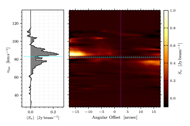
Appendix B \ceSiO maps
Maps of the \ceSiO red- and blue-shifted integrated intensities are shown in Figure 15. Three clumps have clear bipolar outflows: G24051 S5, G28565 S1, and G29601 S1. All three outflows have CO counterparts at similar positions and velocities.
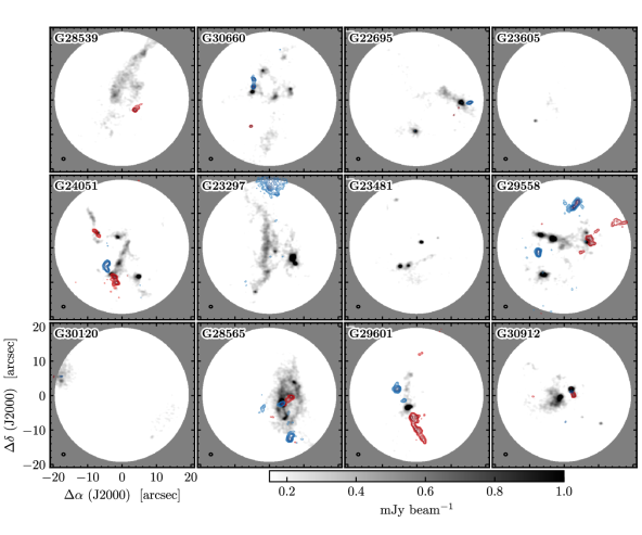
Appendix C Core Model Properties
We follow a similar approach to modeling starless cores as found in Shirley et al. (2005) and Lippok et al. (2016). A similar approach is also used in McGuire et al. (2016). We assume dust opacities for coagulated grains and thin ice mantles in Ossenkopf & Henning (1994, hereafter OH94) for moderately processed grains with a coagulation timescale of at densities between (i.e. “OH4” through “OH6”). The coagulation density from OH94 is selected for each model core based on whether the mean density (weighted by mass) is in the range . The value of the dust opacity when interpolated at for (“OH5a”) is and varies between over the full range of densities. We calculate total the gas mass using a dust-to-gas mass ratio of and an ISM mean molecular weight of . To fully sample the spectral range of the ISRF we extrapolate the the dust opacities from to using the prescription of Cardelli et al. (1989) and from to using the power law with . In addition, scattering efficiencies for the the OH94 models are added following Young & Evans (2005) and albedos from the Weingartner & Draine (2001) WD3.1 model.
The Plummer-like density profile in Eq. (1) is then irradiated in RADMC-3D with an external source input using the spectral energy distribution of the ISRF for a self-consistent calculation of the dust temperature distribution. We use the Black (1994) ISRF spectrum as parametrized by Hocuk et al. (2017, see Appendix B) with the UV portion of the spectrum adopted from Draine (1978). The ISRF is then varied in relative strength from the local value of the solar neighborhood by a multiplicative factor , excluding the contribution from the CMB. Figure 16a shows the ISRF specific intensity for , , and with the five parametrized components clearly visible. Models are computed on a 1D radial grid from with 100 zones with photons to ensure convergence in the output profiles over the tested range in . The median core mass integrated out a radius of is with the percentile interval ranging between , extending to at the 92 percentile. Figure 17 shows the distributions of radial profiles in , , and at a fiducial distance of . The typical at range from and have typical central , with the maximum central .
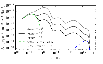
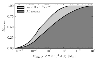
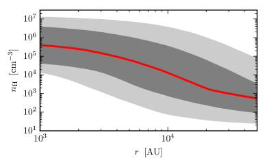
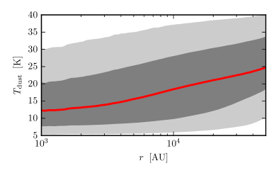
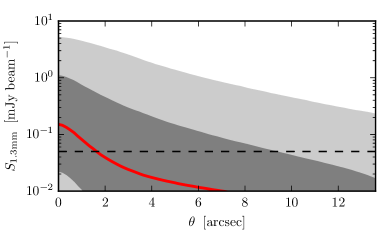
| Name | (ICRS) | (ICRS) | bgps ida | |||
|---|---|---|---|---|---|---|
| (deg) | (deg) | (h:m:s) | (d:m:s) | () | ||
| G22695 | 22.695381 | -0.454657 | 18:34:14.58 | -09:18:35.84 | 77.80 | 3686 |
| G23297 | 23.297388 | 0.055330 | 18:33:32.06 | -08:32:26.27 | 55.00 | 3822 |
| G23481 | 23.479544 | -0.534764 | 18:35:59.56 | -08:39:02.53 | 63.80 | 3892 |
| G23605 | 23.605390 | 0.181325 | 18:33:39.40 | -08:12:33.24 | 87.00 | 3929 |
| G24051 | 24.051381 | -0.214655 | 18:35:54.40 | -07:59:44.60 | 81.10 | 4029 |
| G28539 | 28.538652 | -0.270358 | 18:44:22.60 | -04:01:57.70 | 88.60 | 4732 |
| G28565 | 28.527846 | -0.252172 | 18:44:17.52 | -04:02:02.40 | 87.46 | 4729 |
| G29558 | 29.557855 | 0.185321 | 18:44:37.07 | -02:55:04.40 | 79.72 | 5021 |
| G29601 | 29.604891 | -0.576768 | 18:47:25.20 | -03:13:26.04 | 75.78 | 5030 |
| G30120 | 30.119855 | -1.146674 | 18:50:23.54 | -03:01:31.58 | 65.31 | 5114 |
| G30660 | 30.657875 | 0.044680 | 18:47:07.76 | -02:00:12.17 | 80.20 | 5265 |
| G30912 | 30.913113 | 0.720803 | 18:45:11.28 | -01:28:03.72 | 50.74 | 5360 |
Note. — (a) Catalog ID number in the BGPS v2.1.0 (Ginsburg et al., 2013).
| Name | ||||
|---|---|---|---|---|
| () | () | ( M_⊙) | () | |
| G22695 | 4450 (190) | 0.0580 (0.013) | 930 (110) | 14.70 (0.42) |
| G23297 | 3480 (281) | 0.0760 (0.019) | 420 ( 85) | 11.73 (0.41) |
| G23481 | 3780 (220) | 0.1100 (0.024) | 760 (120) | 11.29 (0.14) |
| G23605 | 4800 (240) | 0.0370 (0.015) | 880 (260) | ( ) |
| G24051 | 4490 (210) | 0.0790 (0.015) | 760 (110) | 11.87 (0.37) |
| G28539 | 4780 (220) | 0.1280 (0.011) | 3610 (360) | 12.38 (0.14) |
| G28565 | 4680 (200) | 0.0830 (0.019) | 910 (220) | ( ) |
| G29558 | 4370 (240) | 0.0690 (0.014) | 590 ( 86) | 12.11 (0.17) |
| G29601 | 4270 (280) | 0.0900 (0.018) | 660 (130) | 15.98 (0.27) |
| G30120 | 3680 (260) | 0.0750 (0.031) | 820 (160) | 14.12 (0.15) |
| G30660 | 4410 (240) | 0.0770 (0.019) | 1380 (360) | ( ) |
| G30912 | 2980 (250) | 0.0990 (0.019) | 450 ( 88) | 11.67 (0.12) |
| spw | Cen. Freq. | Bandwidth | Bandwidth | |||
|---|---|---|---|---|---|---|
| (GHz) | (kHz) | () | (kHz) | () | ||
| 1 | 216.112580 | 960 | 468750.0 | 650.252 | 488.28 | 0.677 |
| 2 | 217.104980 | 960 | 468750.0 | 647.280 | 488.28 | 0.674 |
| 3 | 218.222192 | 480 | 117187.2 | 160.991 | 244.14 | 0.335 |
| 4 | 218.475632 | 480 | 117187.2 | 160.804 | 244.14 | 0.335 |
| 5 | 218.760066 | 480 | 117187.2 | 160.595 | 244.14 | 0.335 |
| 6 | 219.560358 | 240 | 117187.2 | 160.010 | 488.28 | 0.667 |
| 7 | 230.538000 | 960 | 468750.0 | 609.564 | 488.28 | 0.635 |
| 8 | 231.321828 | 960 | 468750.0 | 607.499 | 488.28 | 0.632 |
| 9 | 233.820000 | 128 | 2000000.0 | 2564.301 | 15625.00 | 20.033 |
Note. — Column descriptions: (1) Spectral window (SPW) ID number, (2) Center frequency of SPW in the rest frame, (3) Number of channels, (4,5) SPW total bandwidth, (6,7) SPW channel resolution. Uncertainties are given in parentheses.
| Specie | Transition | Rest Freq. | Ref. | spw | ||
|---|---|---|---|---|---|---|
| (GHz) | (K) | () | ||||
| \ceDCO+ | 216.1125800 | 20.74 | (1) | 1 | 0.68 | |
| c-\ceHC3H | 216.2787560 | 19.47 | (1) | 1 | 0.68 | |
| \ceSiO | 217.1049800 | 31.26 | (1) | 2 | 0.68 | |
| \ceDCN | 217.2385378 | 20.85 | (2) | 2 | 0.68 | |
| p-\ceH2CO | 218.2221920 | 20.96 | (1) | 3 | 0.34 | |
| p-\ceH2CO | 218.4756320 | 68.09 | (1) | 4 | 0.34 | |
| \ceCH3OH | 218.4400500 | 45.46 | (1) | 4 | 0.34 | |
| p-\ceH2CO | 218.7600660 | 68.11 | (1) | 5 | 0.34 | |
| \ceC^18O | 219.5603580 | 15.81 | (1) | 6 | 0.68 | |
| \ceCO | 230.5380000 | 16.60 | (1) | 7 | 0.68 | |
| \ceN2D+ | 231.3218283 | 22.20 | (2) | 8 | 0.68 |
Note. — Transition property reference key: (1) SLAIM, (2) CDMS.
| Name | ID | (ICRS) | (ICRS) | PA | CO | SiO | ||||||
|---|---|---|---|---|---|---|---|---|---|---|---|---|
| (h:m:s) | (d:m:s) | () | () | () | () | () | () | () | ||||
| G22695 | 1 | 18:34:13.7336 | -09:18:36.6910 | 9.30 | 2.597 | 1.213 | 146.0 | 17.284 | 0.109 | 6.414 | 1 | |
| G22695 | 2 | 18:34:14.6345 | -09:18:44.6915 | 16.54 | 3.022 | 1.976 | 126.1 | 9.083 | 0.196 | 1.518 | ||
| G22695 | 3 | 18:34:14.0405 | -09:18:33.7904 | 7.17 | 2.256 | 1.444 | 135.6 | 5.348 | 0.133 | 0.737 | ||
| G23297 | 1 | 18:33:32.1419 | -08:32:25.9306 | 22.70 | 7.853 | 1.461 | 85.5 | 16.431 | 0.309 | 0.727 | ||
| G23297 | 2 | 18:33:31.6164 | -08:32:29.2777 | 2.79 | 1.055 | 0.870 | 72.4 | 11.515 | 0.088 | 6.381 | 2 | |
| G23297 | 3 | 18:33:32.1439 | -08:32:34.3684 | 6.86 | 3.124 | 1.180 | 61.9 | 5.699 | 0.130 | 0.925 | ||
| G23297 | 4 | 18:33:32.3527 | -08:32:38.5247 | 3.77 | 1.880 | 0.911 | 94.0 | 4.139 | 0.066 | 1.906 | 1 | |
| G23297 | 5 | 18:33:31.5694 | -08:32:30.9485 | 0.86 | 0.692 | 0.488 | 148.8 | 2.542 | 0.045 | 3.026 | ||
| G23297 | 6 | 18:33:31.9659 | -08:32:27.1673 | 2.29 | 1.161 | 0.784 | 107.4 | 1.740 | 0.097 | 0.893 | ||
| G23297 | 7 | 18:33:31.6280 | -08:32:22.9146 | 3.53 | 1.982 | 0.798 | 88.6 | 1.645 | 0.099 | 0.472 | ||
| G23481 | 1 | 18:35:59.8961 | -08:39:08.0500 | 2.68 | 0.998 | 0.853 | -164.0 | 3.514 | 0.085 | 2.311 | ||
| G23481 | 2 | 18:35:59.7404 | -08:39:07.8724 | 3.04 | 1.464 | 0.758 | -137.0 | 2.647 | 0.098 | 1.282 | 1 | |
| G23481 | 3 | 18:35:59.9838 | -08:38:48.7847 | 3.02 | 1.513 | 0.806 | 176.9 | 2.529 | 0.046 | 1.263 | ||
| G23481 | 4 | 18:35:59.4861 | -08:39:01.0450 | 2.56 | 0.962 | 0.702 | 176.2 | 2.265 | 0.103 | 2.030 | ||
| G23481 | 5 | 18:35:59.3916 | -08:39:05.8982 | 5.46 | 4.296 | 0.681 | -153.8 | 1.920 | 0.142 | 0.385 | ||
| G23605 | 1 | 18:33:39.9726 | -08:12:39.4169 | 1.88 | 0.938 | 0.651 | 177.4 | 1.371 | 0.058 | 1.197 | ||
| G24051 | 1 | 18:35:54.1219 | -07:59:53.4130 | 13.49 | 2.213 | 1.980 | -168.1 | 12.535 | 0.164 | 5.085 | ||
| G24051 | 2 | 18:35:55.0045 | -07:59:35.7741 | 8.14 | 3.347 | 0.969 | 112.6 | 6.905 | 0.100 | 1.108 | ||
| G24051 | 3 | 18:35:53.9805 | -07:59:58.0198 | 7.95 | 2.563 | 1.491 | 155.0 | 6.397 | 0.077 | 0.924 | ||
| G24051 | 4 | 18:35:54.4771 | -07:59:41.2910 | 11.24 | 3.038 | 1.379 | -176.6 | 5.844 | 0.207 | 1.192 | 1 | |
| G24051 | 5 | 18:35:54.5839 | -07:59:52.2422 | 4.87 | 1.920 | 1.103 | -148.3 | 5.500 | 0.111 | 1.810 | 1 | 1 |
| G24051 | 6 | 18:35:54.9096 | -07:59:40.4092 | 4.36 | 1.417 | 1.011 | 150.3 | 3.820 | 0.100 | 2.154 | 1 | |
| G24051 | 7 | 18:35:54.4693 | -07:59:49.2862 | 4.14 | 1.641 | 0.987 | 62.3 | 3.810 | 0.120 | 1.044 | ||
| G24051 | 8 | 18:35:54.8945 | -07:59:42.6850 | 3.87 | 1.813 | 0.959 | 154.2 | 1.911 | 0.102 | 0.612 | ||
| G24051 | 9 | 18:35:54.3071 | -07:59:43.7882 | 1.42 | 1.354 | 0.487 | 68.1 | 1.057 | 0.076 | 0.643 | ||
| G24051 | 10 | 18:35:54.3750 | -07:59:45.8972 | 1.44 | 1.396 | 0.454 | 55.4 | 1.045 | 0.077 | 0.645 | ||
| G24051 | 11 | 18:35:54.8697 | -07:59:51.3991 | 1.47 | 1.060 | 0.555 | 135.5 | 0.659 | 0.054 | 0.506 | ||
| G28539 | 1 | 18:44:22.2420 | -04:01:44.7142 | 16.35 | 6.175 | 1.334 | 45.3 | 19.114 | 0.121 | 1.842 | ||
| G28539 | 2 | 18:44:22.7348 | -04:01:56.1668 | 8.58 | 2.585 | 1.671 | 73.6 | 5.411 | 0.183 | 0.711 | ||
| G28539 | 3 | 18:44:22.8536 | -04:02:03.2640 | 12.63 | 4.346 | 2.086 | 46.9 | 4.587 | 0.191 | 0.439 | ||
| G28539 | 4 | 18:44:22.3397 | -04:01:54.0246 | 7.39 | 2.372 | 1.682 | 130.3 | 4.055 | 0.156 | 0.603 | ||
| G28539 | 5 | 18:44:22.8195 | -04:02:07.5292 | 2.36 | 1.403 | 0.682 | 80.2 | 1.249 | 0.064 | 0.526 | ||
| G28539 | 6 | 18:44:22.7434 | -04:01:53.8880 | 1.41 | 0.930 | 0.656 | 169.0 | 0.842 | 0.070 | 0.551 | ||
| G28565 | 1 | 18:44:17.2674 | -04:02:03.5257 | 14.00 | 3.641 | 2.023 | 79.3 | 17.943 | 0.226 | 2.499 | 1 | 1 |
| G28565 | 2 | 18:44:16.9912 | -04:02:01.1285 | 3.52 | 2.395 | 0.776 | 89.0 | 3.894 | 0.093 | 0.946 | ||
| G28565 | 3 | 18:44:17.2241 | -04:02:08.5328 | 2.60 | 1.532 | 0.830 | 78.1 | 3.604 | 0.083 | 1.443 | ||
| G28565 | 4 | 18:44:17.1101 | -04:02:09.7546 | 3.33 | 1.914 | 0.810 | 62.9 | 3.087 | 0.082 | 0.827 | ||
| G28565 | 5 | 18:44:17.0529 | -04:01:58.7236 | 1.87 | 1.082 | 0.690 | 143.2 | 2.401 | 0.069 | 1.347 | ||
| G28565 | 6 | 18:44:17.3596 | -04:02:06.5025 | 1.47 | 0.935 | 0.670 | 109.7 | 1.561 | 0.071 | 0.903 | ||
| G29558 | 1 | 18:44:37.5015 | -02:55:12.4812 | 20.09 | 2.432 | 2.174 | -146.5 | 20.697 | 0.184 | 6.613 | ||
| G29558 | 2 | 18:44:37.3029 | -02:55:01.9117 | 4.83 | 1.372 | 1.029 | 161.9 | 10.569 | 0.130 | 4.941 | 1 | |
| G29558 | 3 | 18:44:37.5338 | -02:55:00.8673 | 3.41 | 1.524 | 0.742 | 171.2 | 6.624 | 0.093 | 3.588 | 1 | |
| G29558 | 4 | 18:44:36.6483 | -02:55:02.6587 | 4.40 | 1.548 | 1.109 | 134.4 | 4.624 | 0.114 | 1.666 | ||
| G29558 | 5 | 18:44:37.0267 | -02:55:08.7202 | 6.09 | 2.893 | 1.085 | 125.8 | 1.881 | 0.146 | 0.332 | ||
| G29558 | 6 | 18:44:37.8020 | -02:55:10.4118 | 3.46 | 1.516 | 1.090 | 125.5 | 1.810 | 0.065 | 0.681 | ||
| G29558 | 7 | 18:44:36.6640 | -02:55:00.1446 | 1.87 | 0.937 | 0.766 | 176.3 | 1.688 | 0.070 | 1.116 | ||
| G29558 | 8 | 18:44:36.6775 | -02:54:57.2062 | 3.91 | 1.871 | 1.128 | 171.4 | 1.626 | 0.090 | 0.472 | ||
| G29558 | 9 | 18:44:37.1252 | -02:55:04.1785 | 2.00 | 1.141 | 0.739 | 45.8 | 1.357 | 0.090 | 0.584 | ||
| G29601 | 1 | 18:47:25.3865 | -03:13:29.3698 | 16.05 | 2.547 | 1.728 | 79.6 | 15.771 | 0.240 | 6.686 | 2 | 1 |
| G29601 | 2 | 18:47:25.3644 | -03:13:20.3497 | 4.94 | 1.908 | 1.077 | -140.3 | 2.192 | 0.123 | 0.567 | ||
| G29601 | 3 | 18:47:25.3951 | -03:13:23.8223 | 4.15 | 2.104 | 0.976 | 78.6 | 1.751 | 0.124 | 0.501 | ||
| G29601 | 4 | 18:47:25.5623 | -03:13:24.6212 | 1.69 | 0.999 | 0.716 | 151.3 | 0.541 | 0.074 | 0.341 | ||
| G30120 | 1 | 18:50:24.7282 | -03:01:27.2884 | 1.38 | 0.820 | 0.683 | 147.5 | 3.924 | 0.020 | 2.709 | 1 | |
| G30120 | 2 | 18:50:24.7785 | -03:01:26.1411 | 0.93 | 0.737 | 0.548 | 53.8 | 2.868 | 0.014 | 2.807 | ||
| G30120 | 3 | 18:50:22.9654 | -03:01:43.6061 | 1.61 | 0.912 | 0.680 | -137.5 | 1.232 | 0.034 | 0.854 | ||
| G30660 | 1 | 18:47:07.7985 | -02:00:24.1287 | 27.58 | 5.270 | 2.513 | 66.2 | 15.430 | 0.191 | 0.902 | ||
| G30660 | 2 | 18:47:08.0553 | -02:00:09.6124 | 14.88 | 2.912 | 2.347 | 178.5 | 8.489 | 0.224 | 2.140 | ||
| G30660 | 3 | 18:47:07.8433 | -02:00:04.5482 | 18.40 | 4.397 | 2.139 | 142.3 | 8.257 | 0.219 | 1.318 | ||
| G30660 | 4 | 18:47:07.4677 | -01:59:58.7398 | 11.09 | 3.618 | 1.832 | 52.6 | 7.588 | 0.095 | 0.984 | ||
| G30660 | 5 | 18:47:07.6647 | -02:00:11.1585 | 11.19 | 2.859 | 1.779 | 53.0 | 5.183 | 0.210 | 0.812 | ||
| G30660 | 6 | 18:47:07.3910 | -02:00:09.7055 | 8.59 | 2.296 | 1.622 | 119.3 | 4.896 | 0.162 | 1.128 | ||
| G30912 | 1 | 18:45:11.4745 | -01:28:04.9508 | 44.25 | 4.523 | 3.651 | 51.0 | 27.344 | 0.403 | 2.728 | 1 | |
| G30912 | 2 | 18:45:11.1447 | -01:28:02.2048 | 12.95 | 2.595 | 1.372 | 124.9 | 9.536 | 0.224 | 4.324 | 2 | |
| G30912 | 3 | 18:45:11.9211 | -01:27:55.2127 | 4.29 | 2.778 | 0.976 | 151.1 | 2.249 | 0.069 | 0.682 | ||
| G30912 | 4 | 18:45:11.4095 | -01:27:58.6881 | 4.05 | 2.365 | 1.096 | -161.7 | 1.498 | 0.114 | 0.430 | ||
| G30912 | 5 | 18:45:10.5824 | -01:28:11.8467 | 1.53 | 0.820 | 0.629 | 179.5 | 1.399 | 0.039 | 1.353 | ||
| G30912 | 6 | 18:45:10.9468 | -01:28:09.9788 | 0.83 | 0.600 | 0.516 | 168.0 | 0.360 | 0.045 | 0.518 |
Note. — Column descriptions: (1) Target clump name, (2) sub-structure ID number, (3) centroid right ascension coordinate, (4) centroid declination coordinate, (5) total dendrogram area, (6) Gaussian major FWHM, (7) Gaussian minor FWHM, (8) Gaussian position angle, (9) source integrated flux density, (10) uncertainty in source integrated flux density, (11) source peak flux density, (12) number of bipolar CO outflows, (13) number of bipolar SiO outflows.
| Name | Cont. | Deuteration | Kinematic | High-Excitation | Outflow | |||||||||||
|---|---|---|---|---|---|---|---|---|---|---|---|---|---|---|---|---|
| 1.3 mm | c- | |||||||||||||||
| G28539 | D | W | W | N | D | D | N | W | N | W | D | D | ||||
| G30660 | D | D | N | N | D | D | W | W | D | D | D | D | ||||
| G22695 | D | W | W | N | D | D | D | D | N | D | B | D | ||||
| G23605 | D | N | N | N | D | D | N | W | N | W | D | N | ||||
| G24051 | D | D | D | D | D | D | D | W | D | D | B | B | ||||
| G23297 | D | D | D | W | D | D | D | D | W | D | B | D | ||||
| G23481 | D | N | N | N | D | D | D | D | N | D | B | W | ||||
| G29558 | D | D | W | D | D | D | D | D | D | D | B | D | ||||
| G30120 | W | N | N | N | D | W | N | N | N | W | B | D | ||||
| G28565 | D | D | W | D | D | D | D | D | D | D | B | B | ||||
| G29601 | D | D | W | N | D | D | D | D | W | D | B | B | ||||
| G30912 | D | D | D | W | D | D | D | D | W | D | B | D | ||||
Note. — (a) Detection flags: D detection with , W weak detection with , N non-detection with , and B detection of bipolar outflow. (b) transitions listed in order of , , and .