A Generalized PSS Architecture for Balancing
Transient and Small-Signal Response

Abstract

For decades, power system stabilizers paired with high initial response automatic voltage regulators have served as an effective means of meeting sometimes conflicting system stability requirements. Driven primarily by increases in power electronically-coupled generation and load, the dynamics of large-scale power systems are rapidly changing. Electric grids are losing inertia and traditional sources of voltage support and oscillation damping. The system load is becoming stiffer with respect to changes in voltage. In parallel, advancements in wide-area measurement technology have made it possible to implement control strategies that act on information transmitted over long distances in nearly real time. In this paper, we present a power system stabilizer architecture that can be viewed as a generalization of the standard $\Delta\omega$-type stabilizer. The control strategy utilizes a real-time estimate of the center-of-inertia speed derived from wide-area measurements. This approach creates a flexible set of trade-offs between transient and small-signal response, making synchronous generators better able to adapt to changes in system dynamics. The phenomena of interest are examined using a two-area test case and a reduced-order model of the North American Western Interconnection. To validate the key findings under realistic conditions, we employ a state-of-the-art co-simulation platform to combine high-fidelity power system and communication network models. The benefits of the proposed control strategy are retained even under pessimistic assumptions of communication network performance.

I Introduction

The delicate balance between synchronizing and damping torque components in a synchronous machine creates a conflicting set of stability-oriented exciter performance requirements [1, 2, 3, 4]. Power system stabilizers (PSS) have long played a critical role in satisfying these requirements; however, changes in bulk system dynamics pose challenges to existing control strategies. As inverter-coupled variable generation displaces synchronous machines, electric grids lose inertia and traditional sources of voltage support and oscillation damping. Correspondingly, the rapid growth of power electronic loads may make the system load stiffer with respect to changes in voltage [5, 6]. In parallel with these changes, wide-area measurement systems (WAMS) have transformed power system monitoring. The deployment of phasor measurement units (PMUs) has made it is possible to implement control strategies that act on information transmitted over long distances in nearly real time [7, 8, 9, 10]. Despite the proliferation of inverter-coupled resources, it is projected that synchronous generation will account for a significant fraction of the capacity of large-scale power systems for decades to come [11]. As the dynamics of these systems change, it may become necessary to rethink how synchronous machines are controlled.

In this paper, we derive a new PSS architecture that can be viewed as a generalization of the standard $\Delta\omega$-type stabilizer. This control strategy stems from a time-varying linearization of the equations of motion for a synchronous machine. It utilizes a real-time estimate of the center-of-inertia speed derived from a set of wide-area measurements. The proposed strategy improves the damping of both local and inter-area modes of oscillation. The ability of the stabilizer to improve damping is decoupled from its role in shaping the system response to transient disturbances. Consequently, the interaction between the PSS and automatic voltage regulator (AVR) can be fine-tuned based on voltage requirements. This approach creates a flexible set of trade-offs between transient and small-signal response, making synchronous generators better able to adapt to changes in system dynamics. Analysis and simulation show that this strategy is tolerant of communication delay, traffic congestion, and jitter.

I-A Literature Review

The role that PSSs play in shaping the dynamic system response to severe transient disturbances, such as generator trips, is explored in [12, 13, 14, 15]. In [15], Dudgeon et al. show that the actions of PSSs and AVRs are dynamically interlinked. High initial response AVRs support transient stability but can reduce the damping of electromechanical modes of oscillation. The primary function of PSSs is to improve oscillation damping, but they can also degrade transient stability by counteracting the voltage signal sent to the exciter by the AVR. Managing these interactions through coordinated AVR and PSS design is studied in [16, 17, 18]. In [14], Grondin, Kamwa, et al. present a multi-band PSS compensator aimed at improving transient stability by adding damping to the lowest natural resonant frequency. The objectives of this compensation approach are similar to those we outline in Section II. We present a PSS architecture that features a new type of multi-band compensator that leverages wide-area measurements to achieve amplitude response attenuation.

Employing remote, or global, input signals to improve the performance of power system damping controllers has inspired many research efforts including [19, 20, 21, 22, 23, 24]. In [19], Aboul-Ela et al. propose a PSS architecture with two inputs, a local signal used mainly for damping the local mode and a global signal for damping inter-area modes. For the global signal, [19] considers tie-line active power flows and speed difference signals that provide observability of specific inter-area modes. As stated in [14], the ideal stabilizing signal for a PSS “should be in phase with the deviation of the generator speed from the average speed of the entire system.” To approximate this ideal signal, the rotor speed is typically passed through a washout (highpass) filter, which may insufficiently attenuate steady-state changes in rotor speed and/or introduce excess phase lead into the bottom end of the control band. In contrast, we explore the implications of combining local measurements with a real-time estimate of the center-of-inertia speed.

The research community is actively working to develop simulation techniques for studying the impact of communication networks on power systems. Federated co-simulation environments consist of two or more independent simulation platforms combined so that they exchange data and software execution commands. In [25], Hopkinson et al. present EPOCHS, a co-simulation environment that combined Network Simulator 2 (ns-2) with PSLF and PSCAD/EMTDC. Many subsequent research efforts followed, including [26, 27, 28]. In this paper, the Hierarchical Engine for Large-scale Infrastructure Co-Simulation (HELICS) is employed [28]. We use this state-of-the-art framework to federate a communication network model developed in ns-3 with a power system model developed in the MATLAB-based Power System Toolbox (PST).

I-B Paper Organization

The remainder of this paper is organized as follows. Section II derives a generalization of the standard $\Delta\omega$-type PSS enabled by wide-area measurements. The impact of this control strategy on a two-area test system is examined in Section III. Section IV evaluates how the main results scale to large systems using a reduced-order model of the North American Western Interconnection. In Section IV-C, we study the effect of nonideal communication network performance using co-simulation. Section V summarizes and concludes.

II Proposed Method

The proposed PSS architecture arises from a time-varying linearization of the equations of motion for a synchronous machine. Here we briefly restate some key concepts and definitions from the theory of continuous-time linear time-varying systems. In the control strategy derivation, these concepts will be applied to the nonlinear form of the swing equation.

II-A Linear Time-Varying Systems

Let ${f:\mathbb{R}^{n}\times\mathbb{R}^{m}\rightarrow\mathbb{R}^{n}}$ denote a nonlinear vector field

$$\dot{x}(t)=f(x(t),u(t)),$$ (1)

where ${x(t)\in\mathbb{R}^{n}}$ is the system state at time $t$ and ${u(t)\in\mathbb{R}^{m}}$ the input. Recall that a time-varying linearization of $f$ takes the form

$$\Delta\dot{x}(t)=A(t)\Delta x(t)+B(t)\Delta u(t),$$ (2)

where ${\Delta x(t)=x(t)-\overline{x}(t)}$ and ${\Delta u(t)=u(t)-\overline{u}(t)}$. The time-varying trajectory about which the system is linearized is determined by $\overline{x}(t)$ and $\overline{u}(t)$.

The state-space matrices can be expressed compactly as

$$A(t) =D_{x}f(\overline{x}(t),\overline{u}(t))$$ (3)

$$B(t) =D_{u}f(\overline{x}(t),\overline{u}(t)),$$ (4)

where the operator $D_{x}$ returns the Jacobian matrix of partial derivatives with respect to $x$ evaluated at time $t$, and $D_{u}$ returns the analogous matrix of partials with respect to $u$. In general, the state-space representation is time-varying when $\overline{x}(t)$ and $\overline{u}(t)$ define a nonequilibrium trajectory.

II-B Control Strategy Derivation

This derivation applies the concepts introduced in Section II-A to the equations of motion for a synchronous machine. Stating the nonlinear swing equation in terms of the per-unit accelerating power, we have

$$\dot{\omega}(t)=-\frac{D}{2H}\left[\omega(t)-\omega_{0}\right]+\frac{1}{2H\omega(t)}\left[P_{m}(t)-P_{e}(t)\right],$$ (5)

where $\omega_{0}$ is the per-unit synchronous speed, $D$ the damping coefficient, and $H$ the inertia constant [3, 4]. Linearizing Eq. 5 about a nonequilibrium trajectory yields

$$\begin{split}\Delta\dot{\omega}(t)={}&{-}\left[\frac{D}{2H}+\frac{\overline{P}_{m}(t)-\overline{P}_{e}(t)}{2H\overline{\omega}(t)^{2}}\right]\Delta\omega(t)\\ &\mspace{-4.0mu}+\frac{1}{2H\overline{\omega}(t)}\left[\Delta P_{m}(t)-\Delta P_{e}(t)\right],\end{split}$$ (6)

where ${\Delta\omega(t)=\omega(t)-\overline{\omega}(t)}$, ${\Delta P_{m}(t)=P_{m}(t)-\overline{P}_{m}(t)}$, and ${\Delta P_{e}(t)=P_{e}(t)-\overline{P}_{e}(t)}$.

A new damping coefficient arises from analysis of Eq. 6

$$\mathfrak{D}(t)=D+\frac{\overline{P}_{m}(t)-\overline{P}_{e}(t)}{\overline{\omega}(t)^{2}}.$$ (7)

Using this coefficient, Eq. 6 can be restated as

$$\Delta\dot{\omega}(t)=-\frac{\mathfrak{D}(t)}{2H}\Delta\omega(t)+\frac{1}{2H\overline{\omega}(t)}\left[\Delta P_{m}(t)-\Delta P_{e}(t)\right].$$ (8)

Hence, as with a standard $\Delta\omega$-type stabilizer it is possible to add damping in the LTV reference frame by creating a component of electrical torque that is in phase with the rotor speed deviations. The difference is that the speed deviations are defined such that ${\Delta\omega(t)=\omega(t)-\overline{\omega}(t)}$, where $\overline{\omega}(t)$ is a function of time that tracks changes in the overall system operating point. The time-varying reference $\overline{\omega}(t)$ makes it possible to almost completely wash out steady-state changes in rotor speed from the control error.

II-C Nonequilibrium Speed Trajectory

In this paper, we will examine the implications of treating $\overline{\omega}(t)$ as a real-time estimate of the center-of-inertia speed

$$\overline{\omega}(t)\approx\frac{\sum_{i\in\mathcal{I}}{H_{i}\omega_{i}(t)}}{\sum_{i\in\mathcal{I}}H_{i}},$$ (9)

where $i$ is the unit index and $\mathcal{I}$ the set of all online conventional generators. The right-hand side of Eq. 9 corresponds to the classical center-of-inertia definition, dating back to at least [29]. A related quantity that incorporates the machine apparent power ratings is studied in [30]. This alternative approach may be more effective than Eq. 9 in capturing the discrepancy in size between large and small machines with similar inertia constants.

The question of how to compute $\overline{\omega}(t)$ for real-time control applications is an interesting research problem in itself that is mostly outside the scope of this paper. A promising method is presented in [31]. At the time of this writing, rotor speed measurements are seldom available through wide-area measurement systems; however, a straightforward way of estimating Eq. 9 would be a weighted average of frequency measurements

$$\overline{\omega}(t)=\frac{1}{f_{0}}\sum_{k\in\mathcal{K}}{\alpha_{k}f_{k}(t)},$$ (10)

where $k$ is the sensor index, and $f_{0}$ the nominal system frequency. The frequency signal reported by the $k$th sensor is denoted by $f_{k}(t)$, and the associated weight by $\alpha_{k}$. The weights are nonnegative and sum to one, i.e., ${1^{T}\alpha=1}$. For simplicity, we will consider the arithmetic mean in which ${\alpha_{k}=1/\left|\mathcal{K}\right|}$ for all $k$, where $\left|\mathcal{K}\right|$ denotes the cardinality of $\mathcal{K}$ or simply the number of available sensors. The research contributions presented in this paper do not depend strongly on this choice. There are numerous implementation-related issues posed by any wide-area control scheme, such as how to handle missing or corrupted data. For examples of how these problems may be addressed, see [32, 10].

II-D A Generalization of the $\Delta\omega$-Type PSS

The control strategy implied by Eq. 8 can be generalized to encompass the standard $\Delta\omega$-type PSS. Splitting the linear time-invariant (LTI) control error ${\Delta\omega(t)=\omega_{i}(t)-\omega_{0}}$ into two constituent parts and taking the linear combination yields

$$\Delta\nu(t)\triangleq\beta_{1}\left[\omega_{i}(t)-\overline{\omega}(t)\right]+\beta_{2}\left[\overline{\omega}(t)-\omega_{0}\right],$$ (11)

where $\beta_{1}$ and $\beta_{2}$ are independent tuning parameters restricted to the unit interval. In Section IV, we show how the open-loop frequency response between the input to the exciter and the output of the PSS can be shaped by adjusting these parameters. The first term in Eq. 11 follows directly from Eq. 8, and the second makes it possible to implement a standard $\Delta\omega$-type PSS using the same framework. As in Section II-C, $\overline{\omega}(t)$ is a real-time estimate of the center-of-inertia speed. Fig. 1 shows the block diagram corresponding to this control strategy where $v_{s}$ is the output of the PSS. If necessary, more than one lead-lag compensation stage may be employed.

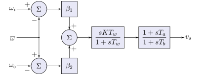
Figure 1: Generalized $\Delta\omega$-type PSS block diagram.

The frequency regulation mode of a power system is a very low-frequency mode, typically below $0.1\text{\,}\mathrm{Hz}$, in which the rotor speeds of all synchronous generation units participate [14, 33]. As a consequence of synchronism, the shape of this mode is such that all conventional generators are in phase with one another. As its name implies, the frequency regulation mode is sensitive to load composition, turbine governor time constants, and droop gains. When ${\beta_{1}>\beta_{2}}$, the control tuning prioritizes the damping of inter-area and local modes of oscillation while de-emphasizing the frequency regulation mode. The converse is true when ${\beta_{1}<\beta_{2}}$. In the special case that ${\beta_{1}=\beta_{2}}$, we have a conventional $\Delta\omega$-type PSS. The resulting control error in this case is exactly the same as in the standard formulation presented in [3]. Table I summarizes the effect of $\beta_{1}$ and $\beta_{2}$ on the PSS tuning.

TABLE I: Effect of Control Parameters on PSS Tuning

Parameter Values	Tuning Description
${\beta_{1}>\beta_{2}}$	Targets inter-area and local modes
${\beta_{1}<\beta_{2}}$	Targets the frequency regulation mode
${\beta_{1}=\beta_{2}\neq 0}$	Standard $\Delta\omega$-type PSS
${\beta_{1}=\beta_{2}=0}$	No PSS control

The diagram shown in Fig. 1 accurately illustrates the control strategy; however, the structure can be clarified further. Expanding the second term in Eq. 11 gives

$$\Delta\nu(t)=\beta_{1}\left[\omega_{i}(t)-\overline{\omega}(t)\right]+\beta_{2}\overline{\omega}(t)-\beta_{2}\omega_{0}.$$ (12)

Thus, we can construct the control error in Eq. 11 with a constant reference and a single feedback signal

$$\Delta\nu(t) =\nu(t)-\nu_{\mathrm{ref}},\ \text{where}$$ (13)

$$\nu_{\mathrm{ref}} =\beta_{2}\omega_{0},\ \text{and}$$ (14)

$$\nu(t) =\beta_{1}\left[\omega_{i}(t)-\overline{\omega}(t)\right]+\beta_{2}\overline{\omega}(t).$$ (15)

The results described in this paper are based on the strategy defined by Eqs. 13 to 15 and illustrated in Fig. 1.

For the sake of completeness, we present a further refinement that permits the per-unit synchronous speed $\omega_{0}$ to serve as the reference. The basic idea is to divide Eq. 12 by $\beta_{2}$, taking care to account for the case where ${\beta_{2}=0}$. Beginning with the control error, we have

$$\Delta\widetilde{\omega}(t)\triangleq\widetilde{\omega}(t)-\omega_{0}.$$ (16)

The feedback signal $\widetilde{\omega}(t)$ is then given by

$$\widetilde{\omega}(t)=\begin{cases}\left(\beta_{1}/\beta_{2}\right)\left[\omega_{i}(t)-\overline{\omega}(t)\right]+\overline{\omega}(t),&\text{for $\beta_{2}>0$}\\[1.0pt] \beta_{1}\left[\omega_{i}(t)-\overline{\omega}(t)\right]+\omega_{0},&\text{for $\beta_{2}=0$}.\end{cases}$$ (17)

This construction is similar to a conventional $\Delta\omega$-type stabilizer where the local speed measurement $\omega_{i}(t)$ has been replaced by $\widetilde{\omega}(t)$. Further illustrating this connection, when $\beta_{1}$ and $\beta_{2}$ are equal and nonzero the feedback signal becomes ${\widetilde{\omega}(t)=\omega_{i}(t)}$. Fig. 2 shows how the simplified PSS block diagram fits in the context of an excitation system with an AVR. This form is equivalent to the one outlined in Eqs. 13 to 15 provided that the downstream gain $K$ is scaled appropriately.

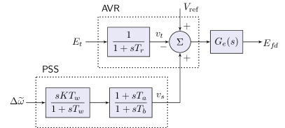
Figure 2: Excitation system with AVR and PSS, where $G_{e}(s)$ represents the transfer function of the exciter.

II-E Comparison With Existing PSS Models

This subsection compares the generalized $\Delta\omega$-type PSS with two industry-standard stabilizer designs: PSS2C and PSS4C. As described in the IEEE recommended practice for excitation system models [34], PSS2C represents a flexible dual-input stabilizer. This model supersedes and is backward compatible with PSS2A and PSS2B. It may be used to represent two distinct implementation types:

1. stabilizers that utilize two inputs to estimate the integral of accelerating power, and

2. stabilizers that utilize rotor speed (or frequency) feedback and incorporate a signal proportional to the electrical power as a means of compensation.

The generalized $\Delta\omega$-type PSS presented here bears similarities to the second of these types. The term in Eq. 11 multiplied by $\beta_{1}$ also represents a local rotor speed combined with an auxiliary signal. The first key difference is that $\overline{\omega}(t)$ in Eq. 11 is synthesized from from wide-area, rather than strictly local, measurements. The second is that the generalized $\Delta\omega$ PSS also provides the ability to independently adjust the amount of steady-state error included in the feedback. In contrast, PSS2C does not feature a multi-band compensation mechanism.

For multi-band compensation, we turn to PSS4C which builds upon the structure originally proposed in [14]. As discussed in Section I-A, the primary difference between the generalized $\Delta\omega$ PSS and PSS4C is the way the compensation is implemented. The PSS4C structure uses parallel lead-lag compensators to delineate the frequency bands, whereas the generalized $\Delta\omega$ PSS uses the linear combination of steady-state and small-signal components in Eq. 11. As shown in Section IV, the latter strategy provides of a means of achieving selective attenuation with minimal impact on the phase response. For an in-depth comparison of PSS2B and PSS4B, the precursors of the models discussed here, see [35].

III Two-Area System Analysis

To study the impact of the control strategy outlined in Section II, a combination of time- and frequency-domain analysis was employed. A custom dynamic model based on the block diagram shown in Fig. 1 was implemented in the MATLAB-based Power System Toolbox (PST) [36]. This application facilitates not only time-domain simulation of nonlinear systems but also linearization and modal analysis. Two test systems were studied: a small model based on the Klein-Rogers-Kundur (KRK) two-area system [37], and a reduced-order model of the Western Interconnection. This section summarizes the results of analyzing the two-area test system. It comprises $13$ buses, $14$ branches, and $4$ synchronous generators. A oneline diagram of the system is shown in Fig. 3. In both models, the active component of the system load is modeled as constant current and the reactive component as constant impedance.

Figure 3: Oneline diagram of the two-area test system.

To permit study of transient disturbances, several modifications were made to the original KRK system. The synchronous machines in the standard case are representative of aggregate groups of generators concentrated in each area. Each unit has the same capacity and inertia. Hence, tripping any one generation unit offline would be equivalent to losing $25\text{\,}\mathrm{\char 37\relax}$ of the rotating inertia online in the system. To facilitate the study of realistically-sized generator trips, the capacity was redistributed such that each area possessed one machine representative of a collection of generators and the other a large individual plant. Generators G$1$ and G$3$ were scaled such that they each represented $5\text{\,}\mathrm{\char 37\relax}$ of the overall system capacity. The remainder was equally split between G$2$ and G$4$. Every unit in the system was then outfitted with the generalized $\Delta\omega$ PSS described in Section II.

III-A Sensitivity of System Poles to the PSS Tuning Parameters

Here we examine the effects of sweeping the PSS tuning parameters $\beta_{1}$ and $\beta_{2}$ on the poles of the system. The modal analysis was performed by linearizing the system dynamics and then solving for the eigenvalues and eigenvectors of the system matrix. The main result is that the oscillatory modes effectively split into two groups, one that is sensitive to changes in $\beta_{1}$ and the other $\beta_{2}$. Let us begin by examining the effect of the tuning parameters on the inter-area and local modes. Consider the inter-area mode indicated by the blue x located at $0.76\text{\,}\mathrm{Hz}$ in Fig. 4. The shape of this mode observed through the machine speeds is shown in Fig. LABEL:sub@fig:mode_shape_inter. Recall that mode shape is defined by the elements of the right eigenvector corresponding to the states of interest [38]. As demonstrated by Fig. LABEL:sub@fig:mode_shape_inter, this mode is characterized by generators G1 and G2 oscillating against G3 and G4. The two-area system is tuned such that this inter-area mode is unstable without supplemental damping control.

(a) $\beta_{1}$ parameter sweep.

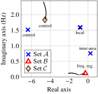
(b) $\beta_{2}$ parameter sweep.

Figure 4: Sensitivity of the system oscillatory modes to the PSS tuning parameters. The modes in $\mathcal{A}$ are sensitive to changes in $\beta_{1}$, those in $\mathcal{B}$ to $\beta_{2}$, and those in $\mathcal{C}$ to both.

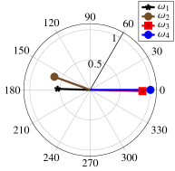
(a) $0.76\text{\,}\mathrm{Hz}$ inter-area mode.

(b) $0.09\text{\,}\mathrm{Hz}$ freq. regulation mode.

Figure 5: Normalized mode shape plots for the two-area system.

The plots in Fig. 4 show the sensitivity of the system poles to the PSS tuning parameters. To generate these plots, either $\beta_{1}$ or $\beta_{2}$ was swept over an interval while the other was held at zero. The tuning parameters for all of the PSS units were swept in unison, and the gain was uniformly held fixed at ${K=25}$. Sweeping the tuning parameters for all units together facilitates study of the effect of PSSs on the frequency regulation mode. In Fig. LABEL:sub@fig:krk_beta1_sensitivity, $\beta_{1}$ was swept over the interval $[0,1]$ while $\beta_{2}$ was held at zero. As $\beta_{1}$ increases, the inter-area mode moves to the left and decreases slightly in frequency. The local modes, indicated by the blue x’s in the upper right quadrant of Fig. LABEL:sub@fig:krk_beta1_sensitivity, move to the left and increase slightly in frequency. A well-controlled exciter mode marked by the blue x in the upper left quadrant moves up and to the right but remains comfortably in the left half of the complex plane. For all intents and purposes, the frequency regulation mode is unaffected by changes in $\beta_{1}$. Hence, $\beta_{1}$ dictates the extent to which the PSS damps inter-area and local modes of oscillation.

The parameter $\beta_{2}$ primarily influences the frequency regulation mode. This mode is indicated by the red triangle located at $0.09\text{\,}\mathrm{Hz}$ in Fig. 4. The shape of the frequency regulation mode observed through the machine speeds is shown in Fig. LABEL:sub@fig:mode_shape_freq. All of the machine speeds are in phase and have nearly identical magnitudes. In Fig. LABEL:sub@fig:krk_beta2_sensitivity, the parameter $\beta_{2}$ was swept over the interval $[0,1]$ while $\beta_{1}$ was held at zero. As $\beta_{2}$ increases, the frequency regulation mode moves to the left. The higher-frequency exciter mode marked with a diamond moves upward. This control mode exhibits some sensitivity to both $\beta_{1}$ and $\beta_{2}$. In contrast, the inter-area and local modes are relatively unaffected by changes in $\beta_{2}$. The dependence of the frequency regulation mode on $\beta_{2}$ indicates that PSSs, in aggregate, play an important role in shaping the system response to transient disturbances. To demonstrate this phenomenon, and the effects of the PSS tuning parameters more broadly, we present a collection of time-domain simulations.

III-B Time-Domain Simulations

The two-area system was simulated in PST for a variety of PSS tunings. As in the frequency-domain analysis, all PSS units were tuned alike and used the same gain. The contingency of interest in this set of simulations is a trip of generator G3. This event was selected because it initiates a transient disturbance that excites not only the inter-area and local modes but also the frequency regulation mode. In the first set of simulations, $\beta_{1}$ was varied over the set $\{0.33,0.67,1\}$ while $\beta_{2}$ was held fixed at $0.33$. In the second set of simulations, $\beta_{1}$ was held fixed at $0.33$ while $\beta_{2}$ was varied over the set $\{0,0.33,0.67\}$. For all simulations, the overall PSS gain was set to ${K=18}$. The case where ${\beta_{1}=\beta_{2}=0.33}$ corresponds to a standard $\Delta\omega$ stabilizer with a gain of ${K=6}$. This set of simulations assumes ideal communication in the construction of the time-varying reference $\overline{\omega}(t)$. Section IV-C addresses the effect of nonideal communication network performance.

Fig. 6 shows the key results for the case where $\beta_{1}$ is varied. The upper subplot shows the difference in speed between generators G2 and G4, i.e., ${\omega_{2}(t)-\omega_{4}(t)}$. The oscillatory content in this signal is dominated by the $0.76\text{\,}\mathrm{Hz}$ inter-area mode. As $\beta_{1}$ increases, the damping of this mode also increases. The lower subplot shows the terminal voltage of generator G4. As $\beta_{1}$ is varied, the large-signal trajectory of the terminal voltage and its post-disturbance value are unchanged. This reflects the fact that varying $\beta_{1}$ only alters the small-signal characteristics of the field current.

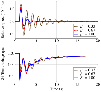
Figure 6: Time-domain simulations of generator G3 being tripped offline for various values of $\beta_{1}$. The top subplot shows the relative speed between G2 and G4.

Fig. 7 shows the key results for the case where $\beta_{2}$ is varied. The upper subplot shows the system frequency response, which readily shows the behavior of the frequency regulation mode. The results show that $\beta_{2}$ plays a key role in determining the depth of the frequency nadir. The frequency nadir improves significantly as $\beta_{2}$ increases from $0$ to $0.33$, and modestly as it goes from $0.33$ to $0.67$. Effectively, $\beta_{2}$ determines the level of overshoot in the system step response. The lower subplot shows the terminal voltage of generator G4. As $\beta_{2}$ is increased, the terminal voltage following the generator trip becomes incrementally more depressed. This can be attributed to the fact that $\beta_{2}$ controls the extent to which steady-state changes in rotor speed are included in the PSS control error.

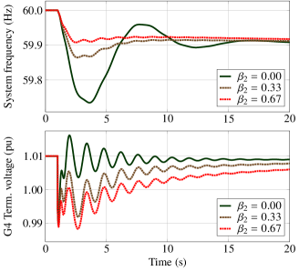
Figure 7: Time-domain simulations of generator G3 being tripped offline for various values of $\beta_{2}$.

The process that causes $\beta_{2}$ to affect the frequency nadir is indirect. Increasing $\beta_{2}$ amplifies the steady-state component of the control error in Eq. 11. This depresses the field current supplied by the exciter and causes the voltage induced in the stator to dip. The electrical load decreases in response to this voltage dip with the amount of relief depending on the sensitivity of the load with respect to voltage. This tends to reduce the time-varying mismatch in mechanical and electrical torque, which improves the frequency nadir. This effect depends on the load composition, and the amount of improvement in the nadir decreases as the fraction of constant power load increases. Thus, there is a trade-off between improving the frequency nadir and degrading the voltage response. As explained in [15], the tendency of the PSS to counteract the voltage signal sent to the exciter by the AVR can reduce synchronizing torque and degrade transient stability. The control strategy presented in this paper makes it possible to fine-tune the interaction between the PSS and AVR without affecting the damping of inter-area and local modes, and vice versa.

IV Large-Scale Test System Analysis

For the two-area system discussed in Section III, the inter-area and local modes were influenced by $\beta_{1}$, and the frequency regulation mode by $\beta_{2}$. This section addresses whether this property is preserved for large-scale systems. We consider a reduced-order model of the Western Interconnection named the miniWECC, in reference to the Western Electric Coordinating Council (WECC). It comprises $122$ buses, $171$ ac branches, $2$ HVDC lines, and $34$ synchronous generators. This system spans the entirety of the interconnection including British Columbia and Alberta. Its modal properties have been extensively validated against real system data [9, 39]. The aim of this analysis is to illustrate the fundamental behavior of various aspects of the proposed architecture in a controlled setting. Prior to implementation, high-fidelity simulation studies that account for variation in PSS structure and the dynamics of inverter-coupled generation would be required.

IV-A Sensitivity of System Poles to the PSS Tuning Parameters

To examine the sensitivity of the oscillatory modes to the PSS tuning parameters, the method described in Section III-A was applied to the miniWECC. Every generation unit in the system was outfitted with a generalized $\Delta\omega$ PSS with the gain set to ${K=25}$. In practice, WECC policy dictates that “a PSS shall be installed on every synchronous generator that is larger than $30\text{\,}\mathrm{MVA}$, or is part of a complex that has an aggregate capacity larger than $75\text{\,}\mathrm{MVA}$, and is equipped with a suitable excitation system” [40]. Fig. 8 shows the movement of the system poles in response to changes in the tuning parameters. In each subplot, either $\beta_{1}$ or $\beta_{2}$ was swept over an interval while the other was held at zero. The main result matches the one observed for the two-area system. The inter-area and local modes are influenced by $\beta_{1}$, and the frequency regulation mode by $\beta_{2}$. For the miniWECC, there is one well-controlled exciter mode near $0.28\text{\,}\mathrm{Hz}$ that exhibits sensitivity to both parameters. This mode is marked in Fig. 8 with a diamond.

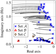
(a) $\beta_{1}$ parameter sweep.

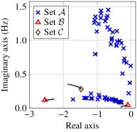
(b) $\beta_{2}$ parameter sweep.

Figure 8: Sensitivity of the miniWECC oscillatory modes to the PSS tuning parameters. The modes in $\mathcal{A}$ are sensitive to changes in $\beta_{1}$, those in $\mathcal{B}$ to $\beta_{2}$, and those in $\mathcal{C}$ to both.

IV-B Open-Loop Frequency Response Analysis

The frequency-domain analysis presented in Sections III and IV-A focused on a system-wide perspective. Here we provide a unit-specific analysis of the open-loop frequency response for a single generator. Outfitting a single unit with a PSS yields the state-space representation

$$\dot{x}(t) =Ax(t)+B_{p}u(t)$$ (18)

$$y_{\nu}(t) =C_{\nu}x(t),$$ (19)

where $B_{p}$ describes how the system states are affected by changes in the PSS control input. The closed-loop control action determined by Eq. 13 can be implemented with the input

$$u(t) =-Ky_{\nu}(t)=-KC_{\nu}x(t)$$ (20)

$$u(t) =-K\begin{bmatrix}0&\gamma_{1}&\gamma_{2}&\dots&-\beta_{1}\end{bmatrix}\begin{bmatrix}\widehat{x}(t)\\ f_{1}(t)\\ f_{2}(t)\\ \vdots\\ \omega_{i}(t)\end{bmatrix},$$ (21)

where $K$ is a scalar gain. The output matrix $C_{\nu}$ combines the states to form the PSS feedback signal $\nu(t)$. Note the presence of the extra negative sign to conform to the negative feedback convention. The state vector $x$ in Eq. 21 is organized with the unused states $\widehat{x}$ on top, followed by the frequency measurements and the local rotor speed. For the $k$th sensor ${\gamma_{k}=\alpha_{k}\left(\beta_{1}-\beta_{2}\right)/f_{0}}$, where $\alpha_{k}$ stems from the linear combination in Eq. 10, and $f_{0}$ is the nominal system frequency. In this analysis, the frequencies were computed by applying a derivative-filter cascade to the bus voltage angles as described in [10]. Hence, the unity-gain open-loop transfer function between a change in the PSS reference $\nu_{\mathrm{ref}}$ and the feedback signal $\nu$ is

$$H(s)=C_{\nu}(sI-A)^{-1}B_{p}.$$ (22)

Fig. 9 shows a high-level block diagram of the feedback loop for a single generation unit outfitted with a generalized $\Delta\omega$ PSS. Here $G_{c}(s)$ represents the PSS, $G_{p}(s)$ the plant, and $F(s)$ the feedback process. The exciter dynamics are included in $G_{p}(s)$, and the input to the plant represents a change in the exciter voltage reference $V_{\mathrm{ref}}$. By commutativity, it holds that

$$H(s)=G_{c}(s)G_{p}(s)F(s)=G_{p}(s)F(s)G_{c}(s).$$ (23)

Hence, the loop transfer function between $\Delta\nu$ and $\nu$ is the same as the transfer function between a change in the exciter voltage reference $V_{\mathrm{ref}}$ and the output of the PSS $v_{s}$. Using this function, we can evaluate the effect of the PSS tuning parameters on the open-loop frequency response. For this analysis, only the unit being studied was outfitted with a PSS.

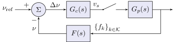
Figure 9: Feedback loop for a single generation unit outfitted with a generalized $\Delta\omega$ PSS, where $G_{c}(s)$ represents the controller, $G_{p}(s)$ the plant, and $F(s)$ the feedback process.

Fig. 10 shows the effect of $\beta_{1}$ on the open-loop frequency response for generator G2, a hydroelectric unit in eastern British Columbia, where ${\beta_{2}=1}$ for all traces. The peak in the amplitude response near $0.04\text{\,}\mathrm{Hz}$ corresponds to the frequency regulation mode. As the plot shows, $\beta_{1}$ has no effect on the gain of the system at this frequency. This corroborates the system-wide modal analysis done in Sections III and IV-A at the unit level. As expected, $\beta_{1}$ does change the amplitude response for the inter-area and local modes of oscillation. Unlike traditional compensation methods, this approach does not degrade the phase response in the attenuation region. As $\beta_{1}$ is varied, the phase response at the frequencies of the dominant amplitude peaks ($0.37\text{\,}\mathrm{Hz}$, $0.62\text{\,}\mathrm{Hz}$, and $1.0\text{\,}\mathrm{Hz}$) is essentially unchanged. The observed transition in phase through $0\text{\,}\mathrm{\SIUnitSymbolDegree}$ at the resonant frequencies is ideal for damping control.

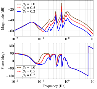
Figure 10: The effect of $\beta_{1}$ on the open-loop frequency response between the input to the exciter and the output of the generalized PSS for generator G2.

Fig. 11 shows the effect of $\beta_{1}$ on the overall PSS compensation. As in [41], the uncompensated open-loop frequency response, including the washout filter dynamics, is provided for comparison. The overall compensation comprises both the lead-lag compensator and the tuning determined by ${\beta_{1},\,\beta_{2}}$. When ${\beta_{1}=\beta_{2}=1}$, the tuning stage has a gain of unity and imparts no phase shift. Hence, all of the compensation stems from the lead-lag compensator. This is expected because the case where ${\beta_{1}=\beta_{2}=1}$ yields a standard $\Delta\omega$ stabilizer as shown in Table I.

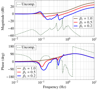
Figure 11: The effect of $\beta_{1}$ on the overall PSS compensation for generator G2 with the washout filter included in the uncompensated frequency response.

Fig. 12 shows the effect of $\beta_{2}$ on the open-loop frequency response where ${\beta_{1}=1}$ for all traces. As $\beta_{2}$ is varied, the amplitude response at the frequencies corresponding to the local and inter-area modes is effectively unchanged. In contrast, the gain at the frequency regulation mode is reduced by roughly $14\text{\,}\mathrm{dB}$ as $\beta_{2}$ goes from $1$ to $0.2$. For ${\beta_{2}=0.2}$, the phase response at the frequency regulation mode leads the case where ${\beta_{2}=1}$ by roughly $35\text{\,}\mathrm{\SIUnitSymbolDegree}$. This suggests that if a $\beta_{2}$ value below some nominal threshold is required for a particular application, it may be necessary to retune the lead-lag compensator and/or washout filter to ensure satisfactory low-frequency performance. The effect of $\beta_{2}$ on the overall PSS compensation is shown in Fig. 13.

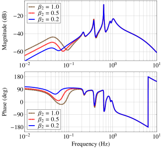
Figure 12: The effect of $\beta_{2}$ on the open-loop frequency response between the input to the exciter and the output of the generalized PSS for generator G2.

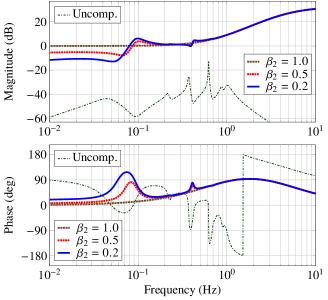
Figure 13: The effect of $\beta_{2}$ on the overall PSS compensation for generator G2 with the washout filter included in the uncompensated frequency response.

IV-C Co-Simulation of Power and Communication Systems

All of the analysis presented in Sections III through IV-B was performed under the assumption of ideal communication. In this section, we analyze the effect of communication delay in the frequency domain and verify the findings in the time domain, as in [42]. The mathematical modeling developed here represents the real-time exchange of synchronized phasor measurement data over a network. As described in the IEEE standard governing data transfer in PMU networks [43], communication delays in WAMS are typically in the range of $20$–$50\text{\,}\mathrm{ms}$; however, the combined delay must also account for the effect of transducers, processing, concentrators, and multiplexing [44, 45, 46]. In [44], the delay attributed to these factors is estimated at $75\text{\,}\mathrm{ms}$, which yields an approximate range of $95$–$125\text{\,}\mathrm{ms}$ for the combined delay. This range is reflective of systems that utilize fiber-optic communication. It aligns closely with the experimental results reported in [10], $69$–$113\text{\,}\mathrm{ms}$, but may vary depending on the communication method employed, e.g., wired vs. wireless. Here we evaluate scenarios with delays that are $5$ to $10$ times greater than the high end of this range.

Modifying the state-space output matrix in Eq. 21 to account for delays as in [47], we have

$$\widehat{C}_{\nu}(s) =\begin{bmatrix}0&\gamma_{1}e^{-s\tau_{1}}&\gamma_{2}e^{-s\tau_{2}}&\dots&-\beta_{1}\end{bmatrix}$$ (24)

$$\widehat{H}(s) =\widehat{C}_{\nu}(s)\left[sI-A\right]^{-1}B_{p},$$ (25)

where $\tau_{k}$ is the delay of the $k$th sensor. Thus, the output matrix changes as a function of frequency. The open-loop transfer function with delay is given by Eq. 25. Fig. 14 shows the results of using Eq. 25 to evaluate the effect of delay on the open-loop frequency response for generator G2 with ${\beta_{1}=1}$ and ${\beta_{2}=0.5}$. For simplicity, ${\tau_{k}=\tau}$ for all $k$. The entries of Eq. 24 correspond to the case where the local signal is not delayed, and the local and remote measurements are not time-aligned upon arrival. As a result, ${\widehat{H}(s)\neq H(s)e^{-s\tau}}$. In the extreme case where ${\tau=$1.25\text{\,}\mathrm{s}$}$ shown in Fig. 14, the gain and phase are altered slightly in the neighborhood of the frequency regulation mode; however, the control performance and stability margins are essentially unchanged.

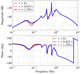
Figure 14: The effect of the combined delay $\tau$ on the open-loop frequency response for generator G2 with ${\beta_{1}=1}$ and ${\beta_{2}=0.5}$.

To study the impact of nonideal communication performance in the time domain, we used a co-simulation framework called HELICS [28]. A communication network model for the miniWECC was developed in ns-3 [48]. It features PMU endpoints that communicate with the controllers via the User Datagram Protocol (UDP). This model includes transmission delay, congesting traffic, and packet-based error emulation. Each generation unit in the PST model was outfitted with a generalized $\Delta\omega$ PSS where ${\beta_{1}=1}$, ${\beta_{2}=0.5}$, and ${K=9}$. Fig. 15 shows time-domain simulations of generator G26, a large nuclear plant in Arizona, being tripped offline for various expected delays $\overline{\tau}$. The results are in close agreement with the frequency-domain analysis shown in Fig. 14. Thus, for this example, the benefits of the control strategy are retained even under pessimistic assumptions of communication network performance.

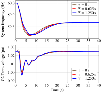
Figure 15: Simulations of generator G26 being tripped offline for various average combined delays where ${\beta_{1}=1}$ and ${\beta_{2}=0.5}$.

In the miniWECC examples discussed herein, the center-of-inertia speed estimate $\overline{\omega}(t)$ was synthesized using $30$ sensors geographically distributed throughout the system. The effect of delay on the open-loop frequency response is dependent on the number and placement of the frequency (or speed) sensors. These factors determine how well $\overline{\omega}(t)$ tracks the target defined in Eq. 9. By extension, they also influence its spectral content. When $\overline{\omega}(t)$ approximately tracks the true center-of-inertia speed, its amplitude spectrum is dominated by very low-frequency content, generally ${\leq\,$0.1\text{\,}\mathrm{Hz}$}$. If too few sensors are used to synthesize this estimate, and/or those sensors are not adequately distributed, the amplitude spectrum of $\overline{\omega}(t)$ may include significant higher-frequency content, in and above the range of the electromechanical modes. If this occurs, the delay may impart larger deviations in the phase response above the frequency regulation mode than shown in Fig. 14. For similar reasons, the coefficients of the linear combination in Eq. 10 also affect the relationship between the combined delay and the frequency response.

The other main factor influencing this relationship is the tuning determined by ${\beta_{1},\,\beta_{2}}$. Analysis indicates that tunings where ${\beta_{1}<\beta_{2}}$ may be more susceptible to the effects of delay than those where ${\beta_{1}\geq\beta_{2}}$. To explore this behavior, we will analyze the entries of the output matrix $\widehat{C}_{\nu}(s)$. Let ${\widehat{\gamma}_{k}=\gamma_{k}/\beta_{1}}$. The matrix $\widehat{C}_{\nu}(s)$ may then be expressed as

$$\widehat{C}_{\nu}(s)=\beta_{1}\begin{bmatrix}0&\widehat{\gamma}_{1}e^{-s\tau_{1}}&\widehat{\gamma}_{2}e^{-s\tau_{2}}&\dots&-1\end{bmatrix},$$ (26)

where

$$\widehat{\gamma}_{k}=\frac{\alpha_{k}}{f_{0}}\left(1-\frac{\beta_{2}}{\beta_{1}}\right).$$ (27)

Recall from Eq. 10 that the weights $\alpha_{k}$ are nonnegative and sum to one. For all real $\omega\tau$, it holds that ${\lvert e^{-j\omega\tau}\rvert=1}$. Thus, the relationship between the magnitudes of the entries of $\widehat{C}_{\nu}(s)$ corresponding to the delayed and non-delayed system states is primarily determined by the ratio $\beta_{2}/\beta_{1}$. Table II shows a breakdown of the possible cases. The term inside the brackets of Eq. 26 corresponding to the local rotor speed always has a magnitude of one. The magnitudes of the remaining entries may either be zero, bounded, or unbounded.

TABLE II: Effect of Control Parameters on $\widehat{\gamma}_{k}$ Coefficients

Parameter Ratio	Coefficient Range
$\begin{aligned} \beta_{2}/\beta_{1}&<1\\ \beta_{2}/\beta_{1}&=1\\ \beta_{2}/\beta_{1}&>1\\ \end{aligned}$	$\begin{aligned} 0&<\widehat{\gamma}_{k}\leq\alpha_{k}/f_{0}\\ 0&\leq\widehat{\gamma}_{k}\leq 0\\ -\infty&\leq\widehat{\gamma}_{k}<0\\ \end{aligned}$

When ${\beta_{2}/\beta_{1}=1}$ the controller is immune to delay because ${\widehat{\gamma}_{k}=0}$ for all $k$. This aligns with expectations because the case where ${\beta_{1}=\beta_{2}\neq 0}$ corresponds to a standard $\Delta\omega$ stabilizer, as shown in Table I. When ${\beta_{2}/\beta_{1}<1}$, the magnitude of $\widehat{\gamma}_{k}$ has an upper bound of $\alpha_{k}/f_{0}$. This corresponds to the case where ${\beta_{1}>\beta_{2}}$, and the PSS prioritizes the damping of local and inter-area modes. When ${\beta_{2}/\beta_{1}>1}$, $\widehat{\gamma}_{k}$ is unbounded below. Thus, the magnitude of $\widehat{\gamma}_{k}$ may grow arbitrarily large as ${\beta_{1}\rightarrow 0}$. This does not imply that $\widehat{C}_{\nu}(s)$ may have infinite values; rather, that the steady-state component of the control error Eq. 11 may be much larger than the small-signal component. This corresponds to the case where ${\beta_{1}<\beta_{2}}$, and the PSS prioritizes shaping the system response to transient disturbances. It is observed that the sensitivity of the open-loop frequency response to delay increases as the ratio $\beta_{2}/\beta_{1}$ increases. We hypothesize that the driving factor in this relationship is that as $\beta_{2}/\beta_{1}$ grows, so too do the magnitudes of the entries of $\widehat{C}_{\nu}(s)$ corresponding to the delayed system states in relation to the non-delayed state(s). That is, when ${\beta_{1}\ll\beta_{2}}$, it follows that ${\lvert\widehat{\gamma}_{k}\rvert>1}$ for some $k$. This suggests that if ${\beta_{1}<\beta_{2}}$, the ratio $\beta_{2}/\beta_{1}$ should be kept small.

To illustrate this behavior, suppose that ${\beta_{1}=0.5}$, ${\beta_{2}=1}$ for generator G2, where ${\beta_{2}/\beta_{1}=2}$. Fig. 16 shows the effect of delay on the open-loop frequency response for G2 in this case. As the delay increases, a key transfer function zero changes position in the complex plane. Fig. 16 indicates that this zero is pushed across the $j\omega$-axis between $0.1$–$0.2\text{\,}\mathrm{Hz}$ and into the right half of the complex plane as the delay increases. Right-half-plane zeros, especially in the neighborhood of the electromechanical modes, may erode stability margins and are generally undesirable [21]. In this case, the system remains stable when ${\tau=$1.25\text{\,}\mathrm{s}$}$ because the gain at the critical frequencies is very low.

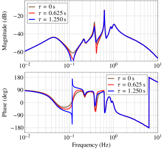
Figure 16: The effect of the combined delay $\tau$ on the open-loop frequency response for generator G2 with ${\beta_{1}=0.5}$ and ${\beta_{2}=1}$.

Fig. 17 shows the system response in the time domain following a trip of G26. Each generation unit in the PST model was outfitted with a generalized $\Delta\omega$ PSS where ${\beta_{1}=0.5}$, ${\beta_{2}=1}$, and ${K=9}$. As the state trajectories show, this tuning places more emphasis on shaping the transient response than on damping local and inter-area modes. Such parameter combinations should be used with caution. Careful stability analysis must be carried out to ensure that it is safe to employ a particular tuning given the performance characteristics of the measurement, communication, and control equipment.

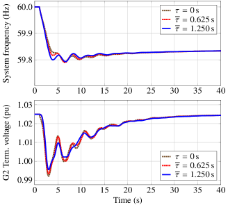
Figure 17: Simulations of generator G26 being tripped offline for various average combined delays where ${\beta_{1}=0.5}$ and ${\beta_{2}=1}$.

V Conclusion

This paper presented a generalization of the standard $\Delta\omega$-type stabilizer. It works by incorporating local information with a real-time estimate of the center-of-inertia speed. The ability of the stabilizer to improve the damping of electromechanical modes is decoupled from its role in shaping the system response to transient disturbances. Hence, the interaction between the PSS and AVR can be fine-tuned based on voltage requirements. Future work will explore a variation of the proposed architecture that permits integral of accelerating power feedback for mitigating torsional oscillations. Finally, another interesting avenue of research will be developing online methods to optimally estimate the center-of-inertia frequency in the presence of delays, jitter, and measurement noise.

Ryan Elliott received the M.S.E.E. degree in 2012 from the University of Washington, Seattle, WA, USA, where he is currently a Ph.D. candidate in the Department of Electrical and Computer Engineering. His research focuses on renewable energy integration, wide-area measurement systems, and power system operation and control. From 2012 to 2015, he was with the Electric Power Systems Research Department at Sandia National Laboratories. While at Sandia, he served on the WECC Renewable Energy Modeling Task Force, leading the development of the WECC model validation guideline for central-station PV plants. In 2017, he earned an R&D 100 Award for his contributions to a real-time damping control system using PMU feedback.

Payman Arabshahi received the Ph.D. degree in 1994 from the University of Washington, Seattle, WA, USA, where he is currently an Associate Professor of Electrical and Computer Engineering and a principal research scientist with the Applied Physics Laboratory. His research focuses on wireless communications and networking, sensor networks, signal processing, data mining and search, and biologically inspired systems. From 1994 to 1996, he served on the faculty of the Electrical and Computer Engineering Department, University of Alabama, Huntsville, AL, USA. From 1997 to 2006, he was on the senior technical staff of NASA’s Jet Propulsion Laboratory in the Communications Architectures and Research Section. While at JPL he also served as affiliate graduate faculty at the Department of Electrical Engineering, California Institute of Technology, Pasadena, CA, USA, where he taught the three-course graduate sequence on digital communications.

Daniel Kirschen received the Electro-Mechanical Engineering degree from the Free University of Brussels, Belgium and the Ph.D. degree from the University of Wisconsin, Madison, WI, USA. He is currently the Donald W. and Ruth Mary Close Professor of Electrical and Computer Engineering at the University of Washington, Seattle, WA, USA. His research focuses on the integration of renewable energy sources in the grid, power system economics, and power system resilience. Prior to joining the University of Washington, he taught for 16 years at the University of Manchester, U.K. Before becoming an academic, he worked for Control Data and Siemens on the development of application software for utility control centers. He has co-authored two books on power system economics and reliability standards for electricity networks.

References

- [1] P. L. Dandeno, A. N. Karas, K. R. McClymont, and W. Watson, “Effect of high-speed rectifier excitation systems on generator stability limits,” IEEE Trans. Power App. Syst., vol. PAS-87, no. 1, pp. 190–201, Jan. 1968.
- [2] F. P. Demello and C. Concordia, “Concepts of synchronous machine stability as affected by excitation control,” IEEE Trans. Power App. Syst., vol. PAS-88, no. 4, pp. 316–329, Apr. 1969.
- [3] P. Kundur, N. Balu, and M. Lauby, Power system stability and control, ser. EPRI Power Systems Engineering. McGraw-Hill, 1994.
- [4] M. Gibbard, P. Pourbeik, and D. Vowles, Small-signal stability, control and dynamic performance of power systems. The University of Adelaide Press, 2015.
- [5] M. Rylander, W. M. Grady, A. Arapostathis, and E. J. Powers, “Power electronic transient load model for use in stability studies of electric power grids,” IEEE Trans. Power Syst., vol. 25, no. 2, pp. 914–921, May 2010.
- [6] L. M. Korunović, J. V. Milanović, S. Z. Djokic, K. Yamashita, S. M. Villanueva, and S. Sterpu, “Recommended parameter values and ranges of most frequently used static load models,” IEEE Trans. Power Syst., vol. 33, no. 6, pp. 5923–5934, Nov. 2018.
- [7] K. Uhlen, L. Vanfretti, M. M. de Oliveira, A. B. Leirbukt, V. H. Aarstrand, and J. O. Gjerde, “Wide-area power oscillation damper implementation and testing in the Norwegian transmission network,” in Proc. IEEE Power Energy Soc. Gen. Meeting, Jul. 2012, pp. 1–7.
- [8] C. Lu, X. Wu, J. Wu, P. Li, Y. Han, and L. Li, “Implementations and experiences of wide-area HVDC damping control in China Southern Power Grid,” in Proc. IEEE Power Energy Soc. Gen. Meeting, Jul. 2012, pp. 1–7.
- [9] D. Trudnowski, D. Kosterev, and J. Undrill, “PDCI damping control analysis for the western North American power system,” in Proc. IEEE Power Energy Soc. Gen. Meeting, Jul. 2013, pp. 1–5.
- [10] B. J. Pierre, F. Wilches-Bernal, D. A. Schoenwald, R. T. Elliott, D. J. Trudnowski, R. H. Byrne, and J. C. Neely, “Design of the Pacific DC Intertie wide area damping controller,” IEEE Trans. Power Syst., vol. 34, no. 5, pp. 3594–3604, Sep. 2019.
- [11] U.S. Energy Information Administration, “Annual energy outlook 2019 with projections to 2050,” EIA/AEO2019, Accessed: July 1, 2019. [Online]. Available: https://www.eia.gov/outlooks/aeo/pdf/aeo2019.pdf
- [12] K. E. Bollinger, R. Winsor, and A. Campbell, “Frequency response methods for tuning stabilizers to damp out tie-line power oscillations: Theory and field-test results,” IEEE Trans. Power App. Syst., vol. PAS-98, no. 5, pp. 1509–1515, Sep. 1979.
- [13] P. Kundur, M. Klein, G. J. Rogers, and M. S. Zywno, “Application of power system stabilizers for enhancement of overall system stability,” IEEE Trans. Power Syst., vol. 4, no. 2, pp. 614–626, May 1989.
- [14] R. Grondin, I. Kamwa, L. Soulieres, J. Potvin, and R. Champagne, “An approach to PSS design for transient stability improvement through supplementary damping of the common low-frequency,” IEEE Trans. Power Syst., vol. 8, no. 3, pp. 954–963, Aug. 1993.
- [15] G. J. W. Dudgeon, W. E. Leithead, A. Dyśko, J. O’Reilly, and J. R. McDonald, “The effective role of AVR and PSS in power systems: Frequency response analysis,” IEEE Trans. Power Syst., vol. 22, no. 4, pp. 1986–1994, Nov. 2007.
- [16] K. T. Law, D. J. Hill, and N. R. Godfrey, “Robust controller structure for coordinated power system voltage regulator and stabilizer design,” IEEE Trans. Control Syst. Technol., vol. 2, no. 3, pp. 220–232, Sep. 1994.
- [17] H. Quinot, H. Bourlès, and T. Margotin, “Robust coordinated AVR+PSS for damping large-scale power systems,” IEEE Trans. Power Syst., vol. 14, no. 4, pp. 1446–1451, Nov. 1999.
- [18] A. Dyśko, W. E. Leithead, and J. O’Reilly, “Enhanced power system stability by coordinated PSS design,” IEEE Trans. Power Syst., vol. 25, no. 1, pp. 413–422, Feb. 2010.
- [19] M. E. Aboul-Ela, A. A. Sallam, J. D. McCalley, and A. A. Fouad, “Damping controller design for power system oscillations using global signals,” IEEE Trans. Power Syst., vol. 11, no. 2, pp. 767–773, May 1996.
- [20] I. Kamwa, R. Grondin, and Y. Hebert, “Wide-area measurement based stabilizing control of large power systems,” IEEE Trans. Power Syst., vol. 16, no. 1, pp. 136–153, Feb. 2001.
- [21] J. H. Chow, J. J. Sanchez-Gasca, H. Ren, and S. Wang, “Power system damping controller design using multiple input signals,” IEEE Control Syst. Mag., vol. 20, no. 4, pp. 82–90, Aug. 2000.
- [22] H. Wu, K. S. Tsakalis, and G. T. Heydt, “Evaluation of time delay effects to wide-area power system stabilizer design,” IEEE Trans. Power Syst., vol. 19, no. 4, pp. 1935–1941, Nov. 2004.
- [23] S. Zhang and V. Vittal, “Design of wide-area power system damping controllers resilient to communication failures,” IEEE Trans. Power Syst., vol. 28, no. 4, pp. 4292–4300, Nov. 2013.
- [24] D. Ke and C. Y. Chung, “Design of probabilistically-robust wide-area power system stabilizers to suppress inter-area oscillations of wind integrated power systems,” IEEE Trans. Power Syst., vol. 31, no. 6, pp. 4297–4309, Nov. 2016.
- [25] K. Hopkinson, X. Wang, R. Giovanini, J. Thorp, K. Birman, and D. Coury, “EPOCHS: A platform for agent-based electric power and communication simulation built from commercial off-the-shelf components,” IEEE Trans. Power Syst., vol. 21, no. 2, pp. 548–558, May 2006.
- [26] H. Lin, S. Veda, S. Shukla, L. Mili, and J. Thorp, “GECO: Global Event-Driven Co-Simulation framework for interconnected power system and communication network,” IEEE Trans. Smart Grid, vol. 3, no. 3, pp. 1444–1456, Sep. 2012.
- [27] S. Ciraci, J. Daily, J. Fuller, A. Fisher, L. Marinovici, and K. Agarwal, “FNCS: A framework for power system and communication networks co-simulation,” in Proc. Symp. Theory Model. & Sim. DEVS Int., Apr. 2014, pp. 1–8.
- [28] B. Palmintier, D. Krishnamurthy, P. Top, S. Smith, J. Daily, and J. Fuller, “Design of the HELICS high-performance transmission-distribution-communication-market co-simulation framework,” in Proc. Model. Sim. Cyber-Phys. Energy Syst., Apr. 2017, pp. 1–6.
- [29] C. J. Távora and O. J. M. Smith, “Characterization of equilibrium and stability in power systems,” IEEE Trans. Power App. Syst., vol. PAS-91, no. 3, pp. 1127–1130, May 1972.
- [30] A. Ulbig, T. S. Borsche, and G. Andersson, “Impact of low rotational inertia on power system stability and operation,” in Proc. 19th IFAC World Congr., Aug. 2014, pp. 7290–7297.
- [31] F. Milano, “Rotor speed-free estimation of the frequency of the center of inertia,” IEEE Trans. Power Syst., vol. 33, no. 1, pp. 1153–1155, Jan. 2018.
- [32] B. Pierre, R. Elliott, D. Schoenwald, J. Neely, R. Byrne, D. Trudnowski, and J. Colwell, “Supervisory system for a wide area damping controller using PDCI modulation and real-time PMU feedback,” in Proc. IEEE Power Energy Soc. Gen. Meeting, Jul. 2016, pp. 1–5.
- [33] F. Wilches-Bernal, J. H. Chow, and J. J. Sanchez-Gasca, “A fundamental study of applying wind turbines for power system frequency control,” IEEE Trans. Power Syst., vol. 31, no. 2, pp. 1496–1505, Mar. 2016.
- [34] “IEEE Recommended practice for excitation system models for power system stability studies,” IEEE Std 421.5-2016, pp. 1–207, Aug. 2016.
- [35] I. Kamwa, R. Grondin, and G. Trudel, “IEEE PSS2B versus PSS4B: The limits of performance of modern power system stabilizers,” IEEE Trans. Power Syst., vol. 20, no. 2, pp. 903–915, May 2005.
- [36] J. H. Chow and K. W. Cheung, “A toolbox for power system dynamics and control engineering education and research,” IEEE Trans. Power Syst., vol. 7, no. 4, pp. 1559–1564, Nov. 1992.
- [37] M. Klein, G. J. Rogers, and P. Kundur, “A fundamental study of inter-area oscillations in power systems,” IEEE Trans. Power Syst., vol. 6, no. 3, pp. 914–921, Aug. 1991.
- [38] G. Rogers, Power system oscillations, ser. Power Electronics and Power Systems. Kluwer Academic Publishers, 1999.
- [39] D. Trudnowski, D. Kosterev, and J. Wold, “Open-loop PDCI probing tests for the western North American power system,” in Proc. IEEE Power Energy Soc. Gen. Meeting, Jul. 2014, pp. 1–5.
- [40] Western Electric Coordinating Council, “WECC policy statement: Power system stabilizers,” Accessed: Sep. 11, 2017. [Online]. Available: https://www.wecc.org/Reliability/WECC%20Policy%20Statement%20on%20Power%20System%20Stabilizers.pdf
- [41] IEEE Power & Energy Society, “IEEE Tutorial course on power system stabilization via excitation control,” Pub. 09TP250, Accessed: June 24, 2019. [Online]. Available: http://sites.ieee.org/pes-resource-center/files/2013/10/09TP250E.pdf
- [42] F. Wilches-Bernal, R. Concepcion, J. C. Neely, D. A. Schoenwald, R. H. Byrne, B. J. Pierre, and R. T. Elliott, “Effect of time delay asymmetries in power system damping control,” in Proc. IEEE Power Energy Soc. Gen. Meeting, Jul. 2017, pp. 1–5.
- [43] “IEEE Standard for synchrophasor data transfer for power systems,” IEEE Std C37.118.2-2011, pp. 1–53, Dec. 2011.
- [44] B. Naduvathuparambil, M. C. Valenti, and A. Feliachi, “Communication delays in wide area measurement systems,” in Proc. 34th Southeastern Symp. on Syst. Theory, Mar. 2002, pp. 118–122.
- [45] S. Zhang and V. Vittal, “Wide-area control resiliency using redundant communication paths,” IEEE Trans. Power Syst., vol. 29, no. 5, pp. 2189–2199, Sep. 2014.
- [46] F. Wilches-Bernal, B. J. Pierre, R. T. Elliott, D. A. Schoenwald, R. H. Byrne, J. C. Neely, and D. J. Trudnowski, “Time delay definitions and characterization in the Pacific DC Intertie wide area damping controller,” in Proc. IEEE Power Energy Soc. Gen. Meeting, Jul. 2017, pp. 1–5.
- [47] F. Wilches-Bernal, D. A. Schoenwald, R. Fan, M. Elizondo, and H. Kirkham, “Analysis of the effect of communication latencies on HVDC-based damping control,” in Proc. IEEE PES Tran. Dist. Conf. Expo., Apr. 2018, pp. 1–9.
- [48] G. F. Riley and T. R. Henderson, The ns-3 Network Simulator. Berlin, Heidelberg: Springer Berlin Heidelberg, 2010, ch. I, pp. 15–34.