Improving Information from Manipulable Data

Data-based decisionmaking must account for the manipulation of data by agents who are aware of how decisions are being made and want to affect their allocations. We study a framework in which, due to such manipulation, data becomes less informative when decisions depend more strongly on data. We formalize why and how a decisionmaker should commit to underutilizing data. Doing so attenuates information loss and thereby improves allocation accuracy.

JEL Classification: C72; D40; D82

Keywords: Gaming; Goodhart’s Law; Strategic Classification

1 Introduction

Firms use a consumer’s web browsing history to price discriminate and to target ads. Banks rely on a prospective borrower’s credit score to make lending decisions. Search engines take as input a website’s text and metadata to produce search results. In these settings and many others, an agent (consumer, borrower, website) generates data that is then used by the designer (firm, bank, search engine) to provide an allocation (prices/ads, interest rates, search rankings). Agents who understand the designer’s algorithm can alter their behavior to receive a more desirable allocation. For instance, consumers can adjust browsing behavior to mimic those with low willingness to pay; borrowers can open or close accounts to improve their credit score; and websites can perform search engine optimization. How should a designer maximize allocation accuracy when accounting for the resulting manipulation?

As a benchmark, consider a naive designer who is unaware of the potential for manipulation. Before implementing an allocation rule, the designer gathers data generated by agents and estimates their types (the relevant characteristics). The naive allocation rule assigns each agent the allocation that is optimal according to this estimate. But after the rule is implemented, agents’ behavior changes: if agents with “higher observables” $x$ receive a “higher allocation” $y$ under the allocation rule $Y(x)$, and if agents prefer higher allocations, then some agents will find ways to game the rule by increasing their $x$. In line with Goodhart’s Law, the original estimation is no longer accurate.

A more sophisticated designer realizes that behavior has changed, gathers new data, and re-estimates the relationship between observables and type. After the designer updates the allocation rule based on the new prediction, agent behavior changes once again. The designer might keep adjusting the rule until she reaches a fixed point: an allocation rule that is a best response to the data that is generated under this very rule. But the resulting allocation need not match the desired agent characteristics well.

In this paper we compare the allocation rule chosen by a designer with commitment power—the Stackelberg solution—to the fixed-point allocation rule. We find that in order to improve the accuracy of allocations, a designer should make the allocation rule less sensitive to manipulable data than under the fixed point. In other words, the designer should “flatten” the allocation rule. Flattening the allocation results in ex-post suboptimality; the designer has committed to “underutilizing” agents’ data. Fixed-point allocations, by contrast, are ex-post optimal. However, a flatter allocation rule reduces manipulation, which makes the data more informative about agents’ types. Allocation accuracy improves on balance. We develop and explore this logic in what we believe is a compelling model of information loss due to manipulation.

By way of background, note that in some environments, manipulation does not lead to information loss: fixed-point rules deliver the designer’s full-information outcome. To see this, think of a fixed-point rule as corresponding to the designer’s equilibrium strategy in a signaling game in which the designer and agent best respond to each other. Under a standard single-crossing condition à la Spence (1973)—the designer wants to give more desirable allocations to agents with higher types, and higher types have lower marginal costs of taking higher observable actions—this signaling game has a fully separating equilibrium, i.e., one in which the designer perfectly matches the agent’s allocation to her type. Even with commitment power, a designer cannot improve accuracy by departing from the corresponding allocation rule.

To introduce information loss, we build on a framework first presented by Prendergast and Topel (1996). The designer learns about an agent’s type by observing data the agent generates, her action $x\in\mathbb{R}$. Agents are heterogeneous on two dimensions of their types, what we call natural action and gaming ability. We initially assume the designer is only interested in the natural action $\eta\in\mathbb{R}$, which determines the agent’s action $x$ absent any manipulation. Gaming ability $\gamma\in\mathbb{R}$ summarizes how much an agent manipulates $x$ in response to incentives. For instance, in the web search application, $x$ represents all that a search engine sees about a website, $\eta$ the fundamental relevance of a website to a given online query, and $\gamma$ how costly it is for a website’s owners to engage in search engine optimization, or how willing they are to do that.

When drawing inferences from the action $x$, the designer’s information about the agent’s natural action $\eta$ is “muddled” with that about gaming ability $\gamma$ (Frankel and Kartik, 2019). We assume the designer observes $x$ and chooses an allocation $y=Y(x)\in\mathbb{R}$ with the goal of minimizing the quadratic distance between $y$ and $\eta$. We restrict attention to linear allocation rules or policies $Y(x)=\beta x+\beta_{0}$, and we posit (with microfoundations) that agents adjust their observable $x$ in proportion to $\gamma\beta$—their gaming ability times the sensitivity of allocations to observables. These linear functional forms arise in the linear-quadratic signaling models of Fischer and Verrecchia (2000) and Bénabou and Tirole (2006), among others.

Our main result establishes that the optimal policy under commitment is less sensitive to observables than is the fixed-point policy. Mathematically, for policies of the form $Y(x)=\beta x+\beta_{0}$, we find that it is optimal for the designer to attenuate the fixed point’s coefficient $\beta>0$ towards zero. (For this discussion, suppose there is a unique fixed point, for which $\beta>0$; our formal analysis addresses the possibility of multiple or negative fixed points.) Information is underutilized at the optimum in the sense that, given the data generated by agents in response to this optimal policy, the designer would ex-post benefit from using a higher $\beta$. For instance, suppose the sensitivity of the naive policy is $\beta=1$: when the designer does not condition the allocation on observables, the linear regression coefficient of type $\eta$ on observable $x$ is 1, and the naive designer responds by matching her allocation rule’s sensitivity to this regression coefficient. The fixed-point policy may have $\beta=0.7$. That is, when the designer sets $\beta=0.7$ and runs a linear regression of $\eta$ on $x$ using data generated by the agent in response to $\beta=0.7$, the regression coefficient is the same $0.7$. Our result is that the optimal policy has $\beta\in(0,0.7)$, say $\beta=0.6$. After the designer sets $\beta=0.6$, however, the corresponding linear regression coefficient is larger than $0.6$, say $0.75$. We emphasize that our argument for shrinking regression coefficients is driven by the informational benefit from reduced manipulation, and in turn, the resulting improvement in allocations. It is orthogonal to concerns about model overfitting.

In comparing our commitment solution with the fixed-point benchmark, it is helpful to keep in mind two distinct interpretations of the fixed point. The first concerns a designer who has market power in the sense that agents adjust their manipulation behavior in response to this designer’s policies. Think of websites engaging in search engine optimization to specifically improve their Google rankings; third party sellers paying for fake reviews on the Amazon platform; or citizens trying to game an eligibility rule for a targeted government policy. In these cases the designer may settle on a fixed point by adjusting policies until reaching an ex-post optimum. Our paper highlights that this fixed point may yet be suboptimal ex ante, and offers the prescriptive advice of flattening the allocation rule.

A second perspective is that the fixed-point policy represents the outcome of a competitive market. With many banks, any one bank that uses credit information in an ex-post suboptimal manner will simply be putting itself at a disadvantage to its competitors; similarly for colleges using SAT scores for admissions. So the fixed point becomes a descriptive prediction of the market outcome, i.e., the equilibrium of a signaling game. In that case, our optimal policy suggests a government intervention to improve allocations, or a direction that collusion might take.

Before turning to the related literature, we stress three points about our approach. First, our paper aims to formalize a precise but ultimately qualitative point, and make salient its logic. Our model is deliberately stylized and, we believe, broadly relevant for many applications. But it is not intended to capture the details on any specific one. We hope that it will be useful for particular applications either as a building block or even simply as a benchmark for thinking about positive and normative implications. Second, we view our main result—the commitment policy flattens fixed points and underutilizes data—as intuitive once one understands the logic of our environment. Indeed, there is a simple first-order gain vs. second-order loss intuition for a local improvement from flattening a fixed point; see Lemma 1 and the discussion after Proposition 2. Confirming that the result holds for the global optimum is not straightforward, however; among other complications, the designer’s problem is not concave and, separately, there can be multiple fixed points. Third, our main result does, of course, depend on certain important modeling assumptions. We emphasize the result because we find the assumptions compelling. Section 4 discusses extensions and limitations, including how the result changes under other assumptions.

Related Literature.

There are many settings in economics in which a designer commits to making ex-post suboptimal allocations in order to improve ex-ante incentives on some dimension. Our specific interest in this paper is in a canonical problem of matching allocations to unobservables in the presence of strategic manipulation. In this context, we study a simple model in which there is a benefit of committing to distortions in order to improve the ex-ante accuracy of the allocations.

Building on the “linear-quadratic-normal” signaling games of Fischer and Verrecchia (2000) and Bénabou and Tirole (2006), Frankel and Kartik (2019) elucidate general conditions under which an agent’s action becomes less informative to an observer when the agent has stronger incentives to manipulate. Frankel and Kartik (2019) model an observer in reduced form: the agent’s payoff is assumed to depend directly on the observer’s belief. In the current paper, we introduce an explicit accuracy objective for the observer/designer. This allows us to consider commitment power for the designer. We compare the commitment optimum with the fixed point, where fixed points correspond to equilibria in the aforementioned signaling-game papers. The key tradeoff our designer faces is suggested by those papers, and also by Prendergast and Topel (1996): making allocations more responsive to an agent’s data amplifies the agent’s manipulation, which makes the data less informative.

Perhaps the most related paper to ours is the contemporaneous work of Ball (2020). He extends the linear-quadratic-elliptical specification in Section IV of Frankel and Kartik (2019) to incorporate multiple “features” or dimensions; on each feature, agents have heterogeneous natural actions and gaming abilities. His main focus is on optimal scoring rules to improve information, specifically in identifying how to weight the different features when aggregating them into a one-dimensional statistic. He also compares his analog of our commitment solution with both his scoring and fixed-point solutions. Similar to our Proposition 2, he finds that under certain conditions, his commitment solution is less responsive to all of an agent’s features than the (unique, under his assumptions) fixed-point solution. He does not study the issues tackled by our Propositions 3–5.

Bjorkegren et al. (2020) present a multiple-features model similar to Ball (2020). Like us, they are interested in the commitment solution. Their emphasis, however, is on empirical estimation; they demonstrate their estimator’s value using a field experiment.

At a very broad level, our main result that the designer should flatten allocations relative to the fixed-point rule is reminiscent of the “downward distortion” of allocations in screening problems following Mussa and Rosen (1978). That said, our framework, analysis, and emphasis—on manipulation and information loss, allocation accuracy, contrasting commitment with fixed points—are not readily comparable with that literature. One recent paper on screening to highlight is Bonatti and Cisternas (2019). In a dynamic price discrimination problem, they show that short-lived firms get better information about long-lived consumers’ types—resulting in higher steady-state profits—if a designer reveals a statistic that underweights recent consumer behavior. Suitable underweighting dampens consumer incentives to manipulate demand.

A finance literature addresses the difficulty of using market activity to learn fundamentals when participants have manipulation incentives. Again in models very different from ours, some papers highlight benefits of committing to underutilizing information. See, for example, Bond and Goldstein (2015) and Boleslavsky et al. (2017). These authors study trading in the shadow of a policymaker who may intervene after observing prices or order flows. The anticipation of intervention makes the financial market less informative about a fundamental to which the intervention should be tailored. Both papers establish that the policymaker may benefit from a commitment that, in some sense, entails underutilization of information. In particular, Bond and Goldstein (2015, Proposition 2) highlight a local first-order information benefit vs. second-order allocation loss akin to our Lemma 1. Unlike us, they do not study global optimality.

A number of papers in economics study the design of testing regimes and other instruments to improve information extraction. Recent examples include Harbaugh and Rasmusen (2018) on pooling test outcomes to improve voluntary participation, Perez-Richet and Skreta (2018) on the benefits of noisy tests when agents can manipulate the test, and Martinez-Gorricho and Oyarzun (2019) on using “conservative” (or “confirmatory”) thresholds to mitigate manipulation. Jann and Schottmüller (2020), Ali and Bénabou (2020), and Frankel and Kartik (2019) analyze how hiding information about agents’ actions—increasing privacy—can improve information about their characteristics.

Beyond economics, our paper connects to a recent computer science literature studying classification algorithms in the presence of strategic manipulation. See, among others, Hardt et al. (2016), Hu et al. (2019), Milli et al. (2018), and Kleinberg and Raghavan (2019). In a binary strategic classification problem, Braverman and Garg (2019) argue for random allocations to improve allocation accuracy and reduce manipulation costs.

We would like to reiterate that our designer is only interested in allocation accuracy, not directly the costs of manipulation. Moreover, unlike Kleinberg and Raghavan (2019), we model an agent’s manipulation effort as pure “gaming”: it does not provide desirable output or affect the designer’s preferred allocation. By contrast to us, principal-agent problems in economics often focus on how allocation rules interact with incentives for desirable effort. For instance, Prendergast and Topel (1996) study contracts in which incentivizing worker effort provides a firm worse information about the worker’s match quality because of an intermediary’s favoritism. In a multitasking environment, Ederer et al. (2018) study how randomized rewards schemes can reduce gaming and improve effort. Liang and Madsen (2020) show that a principal might strengthen an agent’s effort incentives by committing to disregard predictive data acquired from other agents; the benefit can dominate the cost of making less accurate predictions.

2 Model

2.1 The Environment

An agent has a type $(\eta,\gamma)\in\mathbb{R}^{2}$ drawn from joint distribution $F$. It may be helpful to remember the mnemonics $\eta$ for natural action, and $\gamma$ for gaming ability; see Subsection 2.2. Assume the variances $\mathrm{Var}(\eta)=\sigma^{2}_{\eta}$ and $\mathrm{Var}(\gamma)=\sigma^{2}_{\gamma}$ are positive and finite. Denote the means of $\eta$ and $\gamma$ by $\mu_{\eta}$ and $\mu_{\gamma}$, respectively, and assume their correlation is $\rho\in(-1,1)$, with $\rho=\mathrm{Cov}(\eta,\gamma)/(\sigma_{\eta}\sigma_{\gamma})$.

A designer seeks to match an allocation $y\in\mathbb{R}$ to $\eta$, with a quadratic loss of $(y-\eta)^{2}.$ The designer chooses $y=Y(x)$ as a function of an observed action $x\in\mathbb{R}$ that is chosen by the agent. Thus, the designer’s welfare loss is

$$\mathrm{Welfare\ Loss}\equiv\mathbb{E}[(Y(x)-\eta)^{2}].$$ (1)

The agent chooses $x$ as a function of her type $(\eta,\gamma)$ after observing the allocation rule $Y$. In a manner detailed later, the agent will have an incentive to choose a higher $x$ to obtain a higher $y$. Given a strategy of the agent, the designer can compute the distribution of $x$ and the value of $\mathbb{E}[\eta|x]$ for any $x$ the agent may choose. A standard decomposition is

$$\mathrm{Welfare\ Loss} =\underbrace{\mathbb{E}[(\mathbb{E}[\eta|x]-\eta)^{2}]}_{\text{Info loss from estimating $\eta$ using $x$}}+\quad\underbrace{\mathbb{E}[(Y(x)-\mathbb{E}[\eta|x])^{2}]}_{\text{Misallocation loss given estimation}}.$$ (2)

Holding fixed the agent’s strategy, it is “ex-post optimal” for the designer to set $Y(x)=\mathbb{E}[\eta|x]$. However, the agent’s strategy responds to $Y$. So the designer may prefer to use an ex-post suboptimal allocation rule to improve her estimation of $\eta$ from $x$, as seen in the first term of (2). That is, the designer may benefit from the power to commit to her allocation rule.

2.2 Linearity Assumptions

Assume the designer chooses among linear allocation rules: the designer chooses policy parameters $(\beta,\beta_{0})\in\mathbb{R}^{2}$ such that

$$Y(x)=\beta x+\beta_{0}.$$ (3)

Also assume that, given the designer’s policy ($\beta,\beta_{0}$), the agent chooses $x$ using a linear strategy $X_{\beta}(\eta,\gamma)$ that takes the form

$$X_{\beta}(\eta,\gamma)=\eta+m\beta\gamma$$ (4)

for some exogenous parameter $m>0$. Thus $\eta$ is the agent’s “natural action”: the action taken when the designer’s policy does not depend on $x$ (i.e., $\beta=0$). The variable $\gamma$ represents idiosyncratic responsiveness to the designer’s policy: a higher $\gamma$ increases the agent’s action from the natural level by more for any $\beta>0$. The parameter $m$ captures a common component of responsiveness across all agent types.

One can view the agent’s strategy in Equation 4 as a direct behavioral assumption. But it can be microfounded with a number of agent objectives. To begin with, it is the best response for an agent with $\gamma>0$ who maximizes

$$y-(x-\eta)^{2}/(2m\gamma).$$ (5)

Here we refer to $\gamma$ as an agent’s idiosyncratic gaming ability. A higher gaming ability scales down the linear marginal cost of taking actions above the natural action. The parameter $m$ captures the “manipulability” of the action $x$; a higher $m$ scales down marginal costs for all agent types.

A related interpretation is that the agent chooses a level $b$ by which to boost her “baseline output” $\eta$ at cost $b^{2}/(2m\gamma)$, generating output $x=\eta+b$. The agent knows her cost parameter $\gamma$ when choosing $b$ (and may or may not know $\eta$).

Alternatively, with the change of variables $e\equiv(x-\eta)/\sqrt{\gamma}$, the agent’s payoff (5) can be rewritten as $y-e^{2}/(2m)$. The setting is thus isomorphic to one in which the agent chooses “effort” $e$ at a type-independent cost $e^{2}/(2m)$ and the designer observes an outcome $x=\eta+e\sqrt{\gamma}$. Here, $\eta$ can be interpreted as the agent’s baseline talent while $\gamma$ parameterizes her marginal product of effort. When $y=\beta x+\beta_{0}$, the agent optimally chooses $e=m\beta\sqrt{\gamma}$, as per Equation 4.

Finally, the strategy in Equation 4 can also be motivated as the best response for an agent who maximizes a utility of

$$m\gamma y-(x-\eta)^{2}/2.$$

Here $\gamma\in\mathbb{R}$ is an idiosyncratic marginal benefit of obtaining a higher allocation $y$. The parameter $m$ captures the “stakes” common to all agent types.

Remark 1.

The signaling specification in Section IV of Frankel and Kartik (2019), and those in predecessors cited therein, also model an agent behaving as per Equation 4, using the aforementioned microfoundations. They add distributional assumptions on the agent’s type that lead to linear allocation rules (or belief updating, in the signaling context), whereas we assume Equation 3 directly. We study linear allocation rules for their simplicity, tractability, and comparability; see Subsection 4.3 for further discussion.

2.3 The Designer’s Problem

The designer commits to her policy $(\beta,\beta_{0})$, which the agent observes and responds to according to (4). Plugging the rule (3) and the strategy (4) into the welfare loss function (1) yields

$$\mathrm{Welfare\ Loss} =\mathbb{E}[(\beta(\eta+m\beta\gamma)+\beta_{0}-\eta)^{2}].$$

The designer’s problem is therefore to choose $(\beta,\beta_{0})$ to minimize the above loss function, which is quartic in $\beta$. We denote the solution as $(\beta^{*},\beta^{*}_{0})$.

2.4 Discussion

Let us review some of the applications mentioned earlier using the lens of our model.

In one application, the designer is an internet search platform and the agent is the administrator of a website. The site’s true quality—its relevance or value to people searching for certain keywords—is represented by $\eta$. The action or data $x$ is a statistic based on the text and metadata that the platform scrapes off the site. This data can be manipulated through search engine optimization (SEO), with $\gamma$ representing the administrator’s skill at or interest in SEO, or alternatively, the resources the administrator has available. The allocation $y$ is the ultimate search ranking, and the platform seeks to rank better-quality sites higher.

Similarly, the designer may be a sales platform and the agent is a third party seller. There, $\eta$ could be the average rating by genuine users of the product (which proxies for product quality), while the statistic $x$ is the observed rating, which can be manipulated by greedy or unscrupulous sellers (those with high $\gamma$) who pay for fake reviews. Here, negative correlation between $\eta$ and $\gamma$ is plausible: less scrupulous sellers may also tend to cut corners on product quality.

A different application is towards testing, in which a college (the designer) evaluates a student (the agent) based on her test score $x$. The allocation $y$ could represent either the priority ranking for admission or the amount of a merit scholarship; in either case, the student values higher $y$. The student’s type $\eta$ is her intrinsic aptitude or general high school preparation, while the type $\gamma$ is her skill in or support available for “studying to the test”. Here, we might expect $\eta$ and $\gamma$ to be positively correlated: both high school preparation and test-taking resources are aided by better socioeconomic status.

Finally, a firm (the designer) may be allocating a task of importance $y$ to an employee (the agent). The firm seeks to allocate more important tasks to those with more talent, with the employee’s talent given by $\eta$. Recall the “marginal product of effort” interpretation of $\gamma$ from Subsection 2.2: our model can be interpreted as one in which the firm observes the output $x$ of a previous project, with $x=\eta+e\sqrt{\gamma}$ after the employee puts in effort $e$ at cost $e^{2}/(2m)$.

At this point we should highlight that our results in Section 3 depend on the assumption that the designer seeks to match the type dimension $\eta$ rather than $\gamma$. These variables enter asymmetrically into the agent’s behavior in Equation 4. As highlighted in Frankel and Kartik (2019), information about $\eta$ and $\gamma$ can move in opposite directions when the agent is more strongly incentivized to manipulate her action. In the present context, when the designer’s policy puts more weight on the data—when $\beta$ increases—the agent’s action $x$ becomes less informative about $\eta$; see a formalization in Remark 2 below. But the action may simultaneously become more informative about $\gamma$.

In the testing and task allocation applications, a designer could in fact care about $\gamma$ as well as $\eta$. The ability to study for a test, or to increase the output of a project, could be correlated with better performance in future classes or on future tasks. Subsection 4.1 explores how our main result, Proposition 2, extends if the designer places a limited amount of weight on matching $\gamma$ relative to matching $\eta$, but can flip if she places too much weight on matching $\gamma$.

2.5 Preliminaries

2.5.1 Linear regression of type $\eta$ on action $x$

When the designer uses policy $(\beta,\beta_{0})$, the agent responds with strategy $X_{\beta}(\eta,\gamma)=\eta+m\beta\gamma$. To understand better the designer’s welfare loss, suppose the designer were to gather data under that agent behavior and then estimate the relationship between the dimension of interest $\eta$ and the action $x$. Specifically, let $\hat{\eta}_{\beta}(x)$ denote the best linear estimator of $\eta$ from $x$ under a quadratic loss objective:

$$\hat{\eta}_{\beta}(x)\equiv\hat{\beta}(\beta)x+\hat{\beta}_{0}(\beta),$$

with $\hat{\beta}$ and $\hat{\beta}_{0}$ the coefficients of an ordinary least squares (OLS) regression of $\eta$ on $x$. Following standard results for simple linear regressions,

$$\hat{\beta}(\beta) =\frac{\mathrm{Cov}(x,\eta)}{\mathrm{Var}(x)},$$ (6)

$$\hat{\beta}_{0}(\beta) =\mu_{\eta}-\hat{\beta}(\beta)[\mu_{\eta}+m\beta\mu_{\gamma}].$$

Given the strategy $X_{\beta}$, the covariance of $x$ and $\eta$ is $\mathrm{Cov}(x,\eta)=\sigma^{2}_{\eta}+m\rho\sigma_{\eta}\sigma_{\gamma}\beta$ and the variance of $x$ is $\mathrm{Var}(x)=\sigma^{2}_{\eta}+m^{2}\sigma^{2}_{\gamma}\beta^{2}+2m\rho\sigma_{\eta}\sigma_{\gamma}\beta>0$.

It is useful to further rewrite the welfare loss (2) as follows, for any policy $(\beta,\beta_{0})$ defining the linear allocation rule $Y(x)=\beta x+\beta_{0}$:

$$\mathrm{Welfare\ Loss} =\underbrace{\mathbb{E}[(\hat{\eta}_{\beta}(x)-\eta)^{2}]}_{\text{Info loss from linearly estimating $\eta$ using $x$}}+\underbrace{\mathbb{E}[(Y(x)-\hat{\eta}_{\beta}(x))^{2}]}_{\text{Misallocation loss given linear estimation}}.$$ (7)

Some readers may find it helpful to note that information loss from estimation (the first term in (7)) is the variance of the residuals in an OLS regression of $\eta$ on $x$; put differently, $\mathbb{E}[(\hat{\eta}_{\beta}(x)-\eta)^{2}]=\sigma^{2}_{\eta}(1-R^{2}_{x\eta})$, with $R^{2}_{x\eta}$ the coefficient of determination in that regression. Equation 7 is a convenient welfare decomposition for linear allocation rules (given the agent’s linear response) that is valid because OLS provides the best linear predictor of $\eta$ given $x$.

Remark 2.

By a standard property of simple linear regressions, $R^{2}_{x\eta}$ is the square of the correlation between $x$ and $\eta$: $R^{2}_{x\eta}=\mathrm{Corr}(x,\eta)^{2}$. Since $\mathrm{Corr}(x,\eta)=\mathrm{Cov}(x,\eta)/\left(\sigma_{\eta}\sqrt{\mathrm{Var}(x)}\right)$, it is straightforward to confirm using the formulae given earlier for $\mathrm{Cov}(x,\eta)$ and $\mathrm{Var}(x)$ that $\mathrm{Corr}(x,\eta)$ is strictly single peaked in $\beta$ (see Equation A.5 in the Appendix), with a maximum of $\mathrm{Corr}(x,\eta)=1$ when $\beta=0$. Furthermore, $\mathrm{Corr}(x,\eta)\geq 0$ when $\rho\geq 0$ and $\beta\geq 0$. Consequently, at least for $\rho\geq 0$ and $\beta\geq 0$, the designer obtains less information about $\eta$ when she chooses a larger $\beta$.

2.5.2 Benchmark policies

Constant.

A rule that does not condition the allocation on the observable corresponds to a constant policy $(\beta,\beta_{0})$ with $\beta=0$. A constant policy gives rise to a welfare loss of $\sigma^{2}_{\eta}+(\beta_{0}-\mu_{\eta})^{2}$. In the decomposition of Equation 7, the entire welfare loss is due to misallocation; the information loss from estimation is zero because the agent’s behavior $x=\eta$ fully reveals the natural action $\eta$. Under the constant policy the linear estimator $\hat{\eta}_{0}$ has coefficients $\hat{\beta}(0)=1$ and $\hat{\beta}_{0}(0)=0$.

Naive.

If the designer uses a constant policy $(\beta,\beta_{0})$ with $\beta=0$, the agent responds with $X_{0}(\eta,\gamma)=\eta$. Suppose the designer gathers data produced from such behavior, and—failing to account for manipulation—expects the agent to maintain this strategy regardless of the policy. Then the designer would (incorrectly) perceive her optimal policy to be $(\beta^{\mathrm{n}},\beta^{\mathrm{n}}_{0})\equiv(\hat{\beta}(0),\hat{\beta}_{0}(0))=(1,0)$. Alternatively, this would be the designer’s optimum absent any data manipulation (e.g., were $m=0$ instead of our maintained assumption $m>0$).

Designer’s best response.

More generally, suppose the designer expects the agent to use the strategy $X_{\beta}(\eta,\gamma)=\eta+m\beta\gamma$ regardless of the designer’s policy. The designer would find it optimal in response to set an allocation rule $Y(x)$ equal to the best linear estimator of $\eta$ from $x$, i.e., a policy $(\hat{\beta}(\beta),\hat{\beta}_{0}(\beta))$ yielding $Y(x)=\hat{\eta}_{\beta}(x)$.

Fixed point.

We say that a policy $(\beta^{\mathrm{fp}},\beta^{\mathrm{fp}}_{0})$ is a fixed point if

$$\beta^{\mathrm{fp}}=\hat{\beta}(\beta^{\mathrm{fp}})\quad\text{ and }\quad\beta^{\mathrm{fp}}_{0}=\hat{\beta}_{0}(\beta^{\mathrm{fp}}).$$

Fixed points correspond to the pure-strategy Nash equilibria of a game in which the designer’s policy (chosen among linear policies) is set simultaneously with the agent’s strategy (with the agent’s best response given by Equation 4). This simultaneous-move game would eliminate the designer’s commitment power. That is, instead of the designer committing to a policy—the Stackelberg solution—the policy is a best response to the agent’s strategy that the policy induces. Under a fixed-point policy the designer uses information ex-post optimally: in the decomposition of Equation 7, a fixed-point policy has zero misallocation loss.

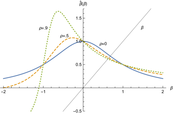
(a) Parameters: $\sigma_{\eta}=\sigma_{\gamma}=1$ and $m=1$.

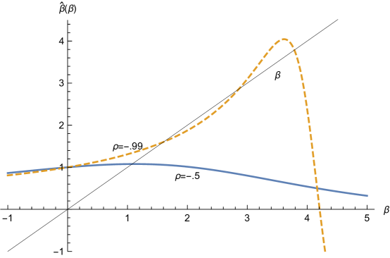
(b) Parameters: $\sigma_{\eta}=\sigma_{\gamma}=1$ and $m=0.24$.

Figure 1: The best response function $\hat{\beta}$. Intersections of $\hat{\beta}$ with $\beta$ correspond to fixed-point sensitivities $\beta^{\mathrm{fp}}$. 1(a) illustrates that when $\rho\geq 0$, $\hat{\beta}$ is decreasing on $[0,\infty)$ and hence there is a unique positive fixed point. 1(b) illustrates that there can be multiple positive fixed points when $\rho<0$.

Figure 1 illustrates some designer best response functions and fixed points. There can, in general, be multiple fixed points, including ones with negative sensitivity or weight on the agent’s action (i.e., $\beta^{\mathrm{fp}}<0$). However, we are interested in, and will focus on, fixed points with positive sensitivity—positive fixed points, for brevity. The following result justifies our focus.

Proposition 1.

Any fixed point has $\beta^{\mathrm{fp}}\neq 0$. There exists a fixed point with $\beta^{\mathrm{fp}}>0$. If $\rho\geq 0$, there is a unique positive fixed point, and it satisfies $\beta^{\mathrm{fp}}\in(0,1)$.

The proof uses a routine analysis of Equation 6. A sensitivity of $\beta=0$ is not a fixed point because $\hat{\beta}(0)=1$. A positive fixed point exists because $\hat{\beta}(\cdot)$ is continuous and $\hat{\beta}(\beta)\to 0$ as $\beta\to\infty$, which reflects that the agent’s action is uninformative about $\eta$ at the limit. The uniqueness result is because nonnegative correlation, $\rho\geq 0$, implies $\hat{\beta}(\cdot)$ is strictly decreasing on $[0,\infty)$, as seen in 1(a). 1(b) illustrates that there can be multiple positive fixed points when $\rho<0$. That there is only one positive fixed point when $\rho\geq 0$ has been noted in different form in Frankel and Kartik (2019, Proposition 4).

Proposition 1 implies that any fixed point has positive information loss: the first term in Equation 7 is positive whenever $\beta\neq 0$. The information loss owes to our maintained assumption that $\sigma_{\gamma}>0$; were $\sigma_{\gamma}=0$, instead, the agent’s strategy from Equation 4 would fully reveal $\eta$ no matter a policy’s sensitivity $\beta$.

3 Analysis

3.1 Main Result

We seek to compare the designer’s optimal policy $(\beta^{*},\beta^{*}_{0})$ with the fixed points $(\beta^{\mathrm{fp}},\beta^{\mathrm{fp}}_{0})$. Take any fixed-point sensitivity $\beta^{\mathrm{fp}}>0$. Our main result, Proposition 2 below, is that the optimal policy puts less weight on the agent’s action than does the fixed point. Furthermore, the optimal policy underutilizes information by putting less weight on the agent’s action than does the OLS coefficient (and hence the best linear policy) given the data generated by the agent in response.

Proposition 2.

There is a unique optimum, $(\beta^{*},\beta^{*}_{0})$. It has $\beta^{*}>0$ and $\beta^{*}<\beta^{\mathrm{fp}}$ for any fixed point with $\beta^{\mathrm{fp}}>0$. Moreover, $\hat{\beta}(\beta^{*})>\beta^{*}$.

For a concrete example, take $m=\sigma^{2}_{\eta}=\sigma^{2}_{\gamma}=1$ and $\rho=0$. Recall that the sensitivity of the naive policy is (normalized to) $\beta=1$. The unique fixed-point policy has $\beta^{\mathrm{fp}}\approx 0.68$. The optimal policy reduces the sensitivity to $\beta^{*}\approx 0.59$. Given the agent’s behavior under this policy, the designer would ex post prefer the higher value $\hat{\beta}(\beta^{*})\approx 0.74$. In this example not only is $\hat{\beta}(\beta^{*})>\beta^{*}$, but $\hat{\beta}(\beta^{*})>\beta^{\mathrm{fp}}$; we explain subsequently that this point holds whenever the correlation $\rho$ is nonnegative.

Here is the intuition for the comparison of the optimum with fixed points, as illustrated graphically in Figure 2. Consider a designer choosing $\beta=\beta^{\mathrm{fp}}>0$. When paired with the correspondingly optimal $\beta_{0}$, this policy is ex-post optimal in the sense that misallocation loss (the second term in the welfare decomposition (7)) given the information the designer obtains about $\eta$ is minimized at zero. Adjusting the sensitivity $\beta$ in either direction from $\beta^{\mathrm{fp}}$ increases misallocation loss, but this harm is second order because we are starting from a minimum. By contrast, at $\beta=\beta^{\mathrm{fp}}$ there is positive information loss from estimation (the first term in (7)) because the agent’s action does not reveal $\eta$. Lowering $\beta$ reduces information loss from estimation, which yields a first-order benefit. (The first-order benefit was suggested by Remark 2 for $\rho\geq 0$, and the point is general, as elaborated below.) Hence, there is a net first-order welfare benefit of lowering $\beta$ from $\beta^{\mathrm{fp}}$. Of course, the designer wouldn’t lower $\beta$ down to 0, since making some use of the information from data is better than not using it at all.

The proof of Proposition 2 in Appendix A establishes uniqueness of the global optimum, rules out that it is negative, and shows that it is less than every fixed point with $\beta^{\mathrm{fp}}>0$. Lemma 1 formalizes a key step, the aforementioned first-order benefit of reducing $\beta$ from any $\beta^{\mathrm{fp}}$. To state the lemma, let $\mathcal{L}(\beta)$ be the welfare loss from policy $\beta$ (paired with the correspondingly optimal $\beta_{0}$), with derivative $\mathcal{L}^{\prime}(\beta)$.

Lemma 1.

For any $\beta^{\mathrm{fp}}$, it holds that $\mathcal{L}^{\prime}(\beta^{\mathrm{fp}})>0$.

Lemma 1 applies regardless of the sign of the correlation parameter $\rho$ and also applies to negative values of $\beta^{\mathrm{fp}}$ when those exist. Here is the logic for the lemma. As noted above, starting from a fixed point the first-order change in welfare loss is just the change in information loss from estimation. Recall from Subsection 2.5.1 that information loss is proportional to $1-R^{2}_{x\eta}$, and $R^{2}_{x\eta}=\mathrm{Corr}(x,\eta)^{2}$. By Equation 6, the sign of $\mathrm{Corr}(x,\eta)$ is that of $\hat{\beta}$, which at a fixed point is the same as the sign of $\beta^{\mathrm{fp}}$. Remark 2 established that, regardless of the sign of $\rho$, $\mathrm{Corr}(x,\eta)$ is increasing in $\beta$ for $\beta<0$ and is decreasing in $\beta$ for $\beta>0$. Putting these facts together, at a positive fixed point $\mathrm{Corr}(x,\eta)$ is positive and locally decreasing in $\beta$, while at a negative fixed point $\mathrm{Corr}(x,\eta)$ is negative and locally increasing in $\beta$. In either case, information loss, which scales with $1-\mathrm{Corr}(x,\eta)^{2}$, is locally increasing in $\beta$.

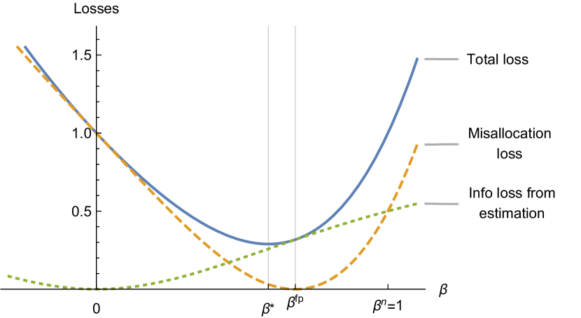
Figure 2: The welfare loss decomposition from Equation 7 for policy $(\beta_{0},\beta)$, with the optimal $\beta_{0}$ plugged in for each $\beta$ on the horizontal axis. Parameters: $\sigma_{\eta}=\sigma_{\gamma}=m=1$ and $\rho=0$. Numerical solutions: $\beta^{*}=0.590$ and $\beta^{\mathrm{fp}}=0.682$.

The last part of Proposition 2 says that information is underutilized at the optimum: $\hat{\beta}(\beta^{*})>\beta^{*}$. The logic for this result can be readily understood using Figure 1. As seen there, $\hat{\beta}(0)>0$, and hence by continuity, $\hat{\beta}(\beta)>\beta$ for all positive $\beta$ less than the smallest positive fixed point. Moreover, as seen in 1(a), $\rho\geq 0$ implies that $\hat{\beta}(\cdot)$ is strictly decreasing on $[0,\infty)$, and hence $\hat{\beta}(\beta^{*})>\beta^{\mathrm{fp}}$ for the unique positive fixed point $\beta^{\mathrm{fp}}$. But the $\rho=-.99$ curve in 1(b) shows that negative correlation can lead to $\hat{\beta}(\beta^{*})<\beta^{\mathrm{fp}}$ for all fixed points $\beta^{\mathrm{fp}}$.

Remark 3.

The welfare gains from commitment can be substantial. As $\rho\to-1$ and for suitable other parameters (viz., $m\sigma_{\gamma}/\sigma_{\eta}\to 1/4^{+}$) the unique fixed point’s welfare is arbitrarily close to that of the best constant policy $Y(x)=\mu_{\eta}$, while the optimal policy’s welfare is arbitrarily close to the first best’s. The welfare of both the first-best policy and the constant policy are independent of $\rho$; the former is $0$ (our normalization) while the latter is $-\sigma^{2}_{\eta}$, which can be arbitrarily low.

Remark 4.

When correlation $\rho$ is nonnegative, the optimal sensitivity $\beta^{*}$ is less than a naive designer’s choice of $\beta=1$ (see Subsection 2.5.2). This follows from the unique positive fixed point satisfying $\beta^{\mathrm{fp}}<1$ when $\rho\geq 0$ (Proposition 1) and $\beta^{*}\in(0,\beta^{\mathrm{fp}})$ (Proposition 2). However, when $\rho<0$ it is possible that $\beta^{*}>1$. In fact, the proof of Proposition 2 yields a characterization: $\beta^{*}<1$ if $2m\sigma_{\gamma}/\sigma_{\eta}>-\rho$; $\beta^{*}>1$ if $2m\sigma_{\gamma}/\sigma_{\eta}<-\rho$; and $\beta^{*}=1$ if $2m\sigma_{\gamma}/\sigma_{\eta}=-\rho$. See Claim A.1 in Appendix A.2.

3.2 Comparative Statics

We provide a few comparative statics below. In taking comparative statics, it is helpful to observe that the designer’s best response $\hat{\beta}(\beta)$ defined in Equation 6 depends on parameters $m$, $\sigma_{\eta}$, and $\sigma_{\gamma}$ only through the statistic $k\equiv m\sigma_{\gamma}/\sigma_{\eta}$, as does the welfare loss $\mathcal{L}(\beta)$ divided by $\sigma^{2}_{\eta}$ (see Equation A.6 in Appendix A.2). Therefore, the optimal and fixed-point values $\beta^{*}$ and $\beta^{\mathrm{fp}}$ also only depend on these parameters through $k$. The statistic $k$ summarizes the susceptibility of the allocation problem to manipulation: higher $k$ (arising from higher stakes or manipulability $m$ of the mechanism, greater variance in gaming ability $\sigma^{2}_{\gamma}$, or lower variance in natural actions $\sigma^{2}_{\eta}$) means that under any given policy, agents adjust their observable action $x$ further from their natural action $\eta$, relative to the spread of observables prior to manipulation. Hence, for comparative statics of $\beta^{*}$ and $\beta^{\mathrm{fp}}$ over model primitives, it is sufficient to consider only the statistic $k$ and the correlation parameter $\rho$.

Proposition 3.

For $k\equiv m\sigma_{\gamma}/\sigma_{\eta}$, the following comparative statics hold for $\beta^{*}$ and $\beta^{*}/\beta^{\mathrm{fp}}$.

1. As $k\to\infty$, $\beta^{*}\to 0$; as $k\to 0$, $\beta^{*}\to 1$. If $\rho\geq 0$, then $\beta^{*}$ is strictly decreasing in $k$; if $\rho<0$, then $\beta^{*}$ is strictly quasiconcave in $k$, attaining a maximum at some point.

2. $\beta^{*}$ is strictly increasing in $\rho$ when $k>3/4$, strictly decreasing in $\rho$ when $k<3/4$, and independent of $\rho$ when $k=3/4$.

3. When $\rho=0$, $\beta^{*}/\beta^{\mathrm{fp}}$ is strictly decreasing in $k$, approaching $\sqrt[3]{1/2}\approx 0.79$ as $k\to\infty$ and $1$ as $k\to 0$.

The limits in part 1 of the proposition are intuitive. From Equation 3 and Equation 4, any particular $\beta>0$ would result in an arbitrarily large allocation for any given type as the manipulability parameter $m\to\infty$ (or, more generally, the statistic $k\to\infty$). Hence, the optimum $\beta^{*}$ must go to $0$ at this limit. As $k\to 0$, by contrast, there is no manipulation, and hence the naive policy becomes optimal: $\beta^{*}\to 1$. Furthermore, when correlation is nonnegative, $\rho\geq 0$, a designer faced with a more manipulable environment (larger $k$) should put less weight on the agent’s action; the intuition is simply that the agent’s action becomes less informative. However, when $\rho<0$, an increase in $k$ can actually make the agent’s action more informative for a given $\beta$. That the optimum $\beta^{*}$ is no longer monotonically decreasing in $k$ follows from the limit $\beta^{*}\to 1$ as $k\to 0$ and Remark 4’s observation that for any $\rho<0$, $\beta^{*}>1$ when $k$ is sufficiently small.

Turning to part 2 of the proposition, one might expect greater correlation to increase the optimum $\beta^{*}$, at least when correlation is nonnegative. But this turns out to hold only when the susceptibility-to-manipulation statistic $k$ is large enough. Here is an explanation. The formal proof shows that the cross partial derivative of welfare loss with respect to $\beta$ and $\rho$ is positive for $\beta$ above a threshold between $0$ and $1$ and negative for $\beta$ below that threshold. When $k$ is small, the designer can restrict attention to values of $\beta$ close to $1$, and hence the optimum is decreasing in $\rho$; when $k$ is large, it is $\beta$ close to $0$ that is relevant, and hence the optimum is increasing in $\rho$.

Finally, part 3 of Proposition 3 implies that when the agent’s characteristics are uncorrelated, the ratio $\beta^{*}/\beta^{\mathrm{fp}}$ decreases as the statistic $k$ increases. As $k\to 0$, the fixed point fully reveals an agent’s natural action ($\beta^{\mathrm{fp}}\to 1$) and so the designer does not benefit from commitment power: the fixed point is optimal as it provides the minimum possible welfare loss. As $k\to\infty$, both $\beta^{*}$ and $\beta^{\mathrm{fp}}$ tend to zero yet the ratio $\beta^{*}/\beta^{\mathrm{fp}}$ stays bounded.

We also have the following comparative statics in welfare:

Proposition 4.

The designer’s welfare loss at the optimum, $\mathcal{L}(\beta^{*})$, is strictly increasing in $\sigma_{\gamma}$ and $m$; it is also strictly increasing in $\sigma_{\eta}$ when $\rho\geq 0$, but for $\rho<0$ it is strictly quasiconvex, attaining a minimum at $\sigma_{\eta}=m\sigma_{\gamma}/(-2\rho)$. Finally, for $\rho\geq 0$, the welfare loss at the optimum is strictly decreasing in $\rho$.

Since the agent’s action is $x=\eta+m\beta\gamma$, it is intuitive that an increase in either $\sigma_{\gamma}$ or $m$ makes actions less informative about $\eta$, and hence reduces the designer’s welfare. Indeed, $\mathcal{L}(\beta^{*})$ divided by $\sigma^{2}_{\eta}$, which is $1-R^{2}_{x\eta}$ (Subsection 2.5.1), depends only on $\rho$ and $k\equiv m\sigma_{\gamma}/\sigma_{\eta}$, and is increasing in $k$; see Lemma A.2 in Appendix A. The effect of an increase in $\sigma_{\eta}$ is more nuanced. Writing welfare loss $\mathcal{L}(\beta^{*})$ as $\sigma^{2}_{\eta}\times\mathcal{L}(\beta^{*})/\sigma^{2}_{\eta}$, we see that increasing $\sigma_{\eta}$ has competing effects: the first term $(\sigma^{2}_{\eta})$ increases due to more baseline uncertainty about $\eta$, whereas the second term ($\mathcal{L}(\beta^{*})/\sigma^{2}_{\eta}$) decreases because spreading out natural actions mutes the noise from heterogenous gaming ability. The first effect unambiguously dominates for $\rho\geq 0$, but it turns out that for any $\rho<0$, if (and only if) $\sigma_{\eta}$ is sufficiently small then the second effect dominates and welfare loss is decreasing in $\sigma_{\eta}$. Finally, the intuition for the welfare loss $\mathcal{L}(\beta^{*})$ decreasing in $\rho$ when $\rho\geq 0$ is that a greater nonnegative correlation is akin to reducing the heterogeneity in gaming ability, which improves information.

4 Discussion

4.1 Mixed Dimensions of Interest

As mentioned in Subsection 2.4, in some settings a designer may care about matching the allocation to not just the agent’s natural action $\eta$ but also the gaming ability $\gamma$. For instance, both dimensions may be predictive of future performance in school or at job tasks. Accordingly, we consider in this subsection (alone) a designer whose welfare loss is given by

$$\mathbb{E}[(Y(x)-\left[(1-\kappa)\eta+\kappa\gamma\right])^{2}],$$ (8)

for some exogenous parameter $\kappa\in(0,1)$. The parameter $\kappa$ reflects the relative importance of gaming ability $\gamma$, compared to a $1-\kappa$ weight on natural action $\eta$.

When considering objective (8), we continue to assume the designer uses linear policies of the form $Y(x)=\beta x+\beta_{0}$ and the agent responds according to $X_{\beta}(\eta,\gamma)=\eta+m\beta\gamma$. The optimal policy now minimizes (8). Just as in Subsection 2.5.1, given any $X_{\beta}$ the designer can calculate $\left(\hat{\beta}(\beta),\hat{\beta}_{0}(\beta)\right)$ as the OLS regression coefficients of $(1-\kappa)\eta+\kappa\gamma$ on $x$. A fixed-point policy $(\beta^{\mathrm{fp}},\beta^{\mathrm{fp}}_{0})$ is one in which $\beta^{\mathrm{fp}}=\hat{\beta}(\beta^{\mathrm{fp}})$ and $\beta^{\mathrm{fp}}_{0}=\hat{\beta}_{0}(\beta^{\mathrm{fp}})$.

The key intuition underlying our main result—when the designer cares only about matching $\eta$, it is optimal to reduce allocation sensitivity from a fixed point—is that decreasing manipulation incentives improves information about $\eta$ (Lemma 1). If the designer cared instead only about matching $\gamma$, the logic from Frankel and Kartik (2019) suggests the opposite should hold. Intuitively, when the allocation sensitivity $\beta>0$ is larger, the variation in the observable $x$ $(=\eta+m\beta\gamma)$ depends more on $\gamma$ and less on $\eta$; hence, increasing manipulation incentives increases information about $\gamma$. Put differently, when the designer cares only about matching $\gamma$, variation in $\eta$ simply adds noise to $x$; increasing $\beta$ effectively scales down that noise.

More generally, one might expect that a designer who puts sufficient weight on matching $\eta$ would optimally reduce the sensitivity from a fixed point, while a designer who weights matching $\gamma$ sufficiently would increase the sensitivity. We can establish such a result cleanly under the simplifying assumption that $\eta$ and $\gamma$ are uncorrelated, i.e., $\rho=0$.

Proposition 5.

Assume $\rho=0$ and designer welfare loss (8). There is a unique fixed point among those with positive sensitivity, which we denote $(\beta^{\mathrm{fp}},\beta^{\mathrm{fp}}_{0})$. Let $\overline{\kappa}\equiv 1-\frac{\sqrt{1+4m}-1}{2m}$ $\in(0,1)$. It holds for the unique optimum $(\beta^{*},\beta^{*}_{0})$ that:

$$\kappa<\overline{\kappa} \implies\beta^{*}\in(0,\beta^{\mathrm{fp}}),$$

$$\kappa=\overline{\kappa} \implies\beta^{*}=\beta^{\mathrm{fp}},$$

$$\kappa>\overline{\kappa} \implies\beta^{*}>\beta^{\mathrm{fp}}.$$

For $\rho=0$, the proposition explicitly identifies identifies a critical threshold, $\overline{\kappa}\in(0,1)$, such that the fixed point with $\beta^{\mathrm{fp}}>0$ is (only) optimal when the designer’s weight on matching $\gamma$ is $\kappa=\overline{\kappa}$. When $\kappa<\overline{\kappa}$, it is optimal to flatten the fixed point; when $\kappa>\overline{\kappa}$, it is optimal to steepen. These conclusions extend and qualify Proposition 2. Interestingly, the threshold weight $\overline{\kappa}$ is increasing in the manipulation parameter $m$, but does not depend on the variances $\sigma^{2}_{\eta}$ and $\sigma^{2}_{\gamma}$.

4.2 Additional Designer Objectives

Information about the agent’s type might only affect part of the designer’s welfare. Our maintained assumption is that agents shift their action by $m\beta\gamma$ away from their natural action. If the designer seeks to induce higher actions, then the designer will commit to increase $\beta$ above the optimum that was based on allocation accuracy. This could occur in the task allocation application where the action $x$ corresponds to the output of an evaluation task—this output may be directly valuable to the firm. The designer would have the same incentives in the school testing application if she didn’t care per se about a student’s test score $x$, but cared about inducing the student to put in effort ($e=(x-\eta)/\sqrt{\gamma}$) to study for the exam.

If the designer instead wants to reduce the agent’s distortions, or the designer internalizes the costs of distortion, she will weaken manipulation incentives by attenuating $\beta$ towards zero. This would be relevant to a government choosing the eligibility rule for a targeted policy. A government that values citizens’ welfare is harmed by the costly effort devoted to gaming eligibility.

Under either of the additional objectives mentioned in the two previous paragraphs, the designer’s ex-post preference—given the agent’s action—remains to match the allocation to the agent’s type. Thus, fixed points are unaffected. So when the designer wants to reduce manipulation costs, our main point on reducing allocation sensitivity from a fixed point is strengthened. But when the designer wants to induce higher actions, the result could reverse.

4.3 Linear Policies

That the designer uses linear allocation rules is generally restrictive. We nevertheless think it is interesting to focus on such policies for reasons beyond their analytical tractability.

First, linear policies are simple, canonical, and practical. As we have explained, they can be studied using linear regressions, which are widely used for estimating the relationship between agent characteristics and observable data.

Second, linear policies are straightforward to interpret. Specifically, they are (up to a constant) fully ordered by the allocation’s sensitivity to data. We can therefore discuss what it means it means for a policy to be “flatter”, i.e., less sensitive to data, and compare the optimum to fixed points in this respect. Furthermore, it allows us to discuss how the designer optimally underutilizes data.

Third, and relatedly, linear policies are focal for comparison with linear fixed points. Gesche (2019) and Frankel and Kartik (2019) have shown that fixing any linear strategy for the agent, the designer’s best response is linear if the agent’s type distribution is bivariate elliptical (Gómez et al., 2003), subsuming bivariate normal; see also Fischer and Verrecchia (2000) and Bénabou and Tirole (2006). Ball (2020) extends these results to a multidimensional action space. Hence, under these joint distributions—and when agents optimally respond to linear allocation rules with linear strategies (see Subsection 2.2)—linear fixed-point policies of the current paper are fixed points even when the designer and the agent choose arbitrary (possibly nonlinear) strategies $Y(x)$ and $X(\eta,\gamma)$.

5 Conclusion

To recap: how should a designer with market power choose an allocation rule to maximize allocation accuracy, given that the rule affects agents’ manipulation of the very data used for allocation? Our main result is that the designer should commit to underutilizing information. The optimal allocation rule is flatter than a fixed-point, or ex-post optimal, rule.

Consider a large search engine like Google that aims to provide its users with an accurate list of organic search results. Our result suggests that Google’s algorithm ought to be less responsive to webpage elements susceptible to search engine optimization (SEO) than if it were to take as given the extent of SEO. An analogous point holds for Amazon’s use of consumer reviews.

Another application concerns standardized testing for college or high school admissions. Our result says that when students can study to the test, the accuracy of admissions can be improved by underutilizing the information contained in test results. However, when there are many decentralized colleges, we would expect each to have limited market power. Thus, each college would tend to use test information ex-post optimally, resulting in less-accurate admissions. One may extrapolate that the more competitive the college sector is, the lower the resulting accuracy.

In various applications, the data that designers have access to is multidimensional. Our results would suggest that a designer should flatten the allocation rule more on dimensions that are more manipulable. Thus, observables that are difficult for the agent to manipulate become relatively more important for the designer’s decision than those that are easy to manipulate. For instance, compared to the ex-post optimum, credit scores should put relatively more weight on the length of a consumer’s credit history and less on the current credit utilization rate when the former is less manipulable. See Ball (2020) for some recent work in this direction.

A notable point is that information loss in our model stems from agents’ heterogeneous responses to incentives. That is, it is not simply the existence of SEO and studying to the test that produces our implications for search engines and college admissions; rather, it is because some website managers engage in more SEO and some students have better access to test preparation. Having said that, the rationale for flattening allocations is not restricted to this source of information loss. For instance, even a model with a one-dimensional type (e.g., no heterogeneity on our gaming ability $\gamma$) may have information loss from “pooling at the top” in a bounded action space. This could be relevant to test taking when there is a binding upper bound on the test score. Appendix C establishes a version of our flattening result for a simple model in that vein.

As we have discussed, linear designer policies and agent responses are a benchmark for understanding how to improve (the use of) information from manipulable data. An interesting topic for future research is the generalization of “flattening” allocations and “underutilizing” information to nonlinear models.

Appendix A Appendix: Proofs

A.1 Proof of Proposition 1

Recall from Subsection 2.5.1 that $\hat{\beta}(\beta)=\mathrm{Cov}(x,\eta)/\mathrm{Var}(x)$, with

$$\mathrm{Cov}(x,\eta) =\sigma^{2}_{\eta}+m\rho\sigma_{\eta}\sigma_{\gamma}\beta,$$ (A.1)

$$\mathrm{Var}(x) =\sigma^{2}_{\eta}+m^{2}\sigma^{2}_{\gamma}\beta^{2}+2m\rho\sigma_{\eta}\sigma_{\gamma}\beta.$$ (A.2)

For $\beta\geq 0$, the fixed-point equation $\hat{\beta}(\beta)=\beta$ can thus be rewritten as the cubic equation

$$m^{2}\sigma^{2}_{\gamma}\beta^{3}+2m\rho\sigma_{\eta}\sigma_{\gamma}\beta^{2}+(\sigma^{2}_{\eta}-m\rho\sigma_{\eta}\sigma_{\gamma})\beta-\sigma^{2}_{\eta}=0.$$ (A.3)

The left-hand side of (A.3) is continuous, negative at $\beta=0$ and tends to $\infty$ as $\beta\to\infty$. There is a positive solution to (A.3) by the intermediate value theorem.

We now show that $\hat{\beta}(\beta)$ is strictly decreasing on $[0,\infty)$ when $\rho\geq 0$. Differentiating Equation A.2 yields

$$\frac{\mathrm{d}}{\mathrm{d}\beta}\mathrm{Var}(x)=2m^{2}\sigma^{2}_{\gamma}+2m\rho\sigma_{\eta}\sigma_{\gamma}.$$ (A.4)

Dividing Equation A.1 by $\sigma_{\eta}\sqrt{\mathrm{Var}(x)}$ and differentiating yields

$$\frac{\mathrm{d}}{\mathrm{d}\beta}\mathrm{Corr}(x,\eta)=-\frac{\beta m^{2}(1-\rho^{2})\sigma_{\eta}\sigma_{\gamma}^{2}}{\mathrm{Var}(x)^{3/2}}.$$ (A.5)

Equation 6 implies that $\hat{\beta}=\mathrm{Corr}(x,\eta)\sigma_{\eta}/\sqrt{\mathrm{Var}(x)}$. For $\rho\geq 0$ and $\beta\geq 0$, Equation A.4 and Equation A.5 respectively show that $\mathrm{Var}(x)$ is strictly increasing and $\mathrm{Corr}(x,\eta)$ is strictly decreasing in $\beta$. The desired conclusion follows.

A.2 Proof of Proposition 2

From Subsection 2.3, $(\beta^{*},\beta^{*}_{0})$ solves

$$\min_{(\beta,\beta_{0})\in\mathbb{R}^{2}}\ \mathbb{E}[(m\beta^{2}\gamma+\beta_{0}-(1-\beta)\eta)^{2}].$$

The first-order condition with respect to $\beta_{0}$ implies

$$\beta_{0}^{*} =(1-\beta)\mu_{\eta}-m\beta^{2}\mu_{\gamma}.$$

Substituting $\beta_{0}^{*}$ into the objective, the designer chooses $\beta$ to minimize

$$\mathbb{E}[(m\beta^{2}(\gamma-\mu_{\gamma})-(1-\beta)(\eta-\mu_{\eta}))^{2}]$$

$$= (1-\beta)^{2}\sigma^{2}_{\eta}+m^{2}\beta^{4}\sigma^{2}_{\gamma}-2(1-\beta)m\beta^{2}\rho\sigma_{\eta}\sigma_{\gamma}$$

$$= \sigma^{2}_{\eta}\left[\left((1-\beta)-k\beta^{2}\right)^{2}+2(1-\rho)\beta^{2}(1-\beta)k\right],$$

where

$$k\equiv m\sigma_{\gamma}/\sigma_{\eta}>0.$$

Equivalently, for $k>0$ and $\rho\in(-1,1)$, $\beta^{*}$ minimizes

$$L(\beta,k,\rho)\equiv\left(k\beta^{2}+\beta-1\right)^{2}+2(1-\rho)\beta^{2}(1-\beta)k.$$ (A.6)

Differentiating,

$${L}_{\beta}(\beta,k,\rho)=-2(1-\beta)+4k^{2}\beta^{3}+2\rho k\beta(3\beta-2).$$ (A.7)

Note that $L_{\beta}(0,k,\rho)<0$, i.e., there is a first-order benefit from putting some positive weight on the agent’s action.

The last statement of Proposition 2 follows from the second because, from Equation 6, $\hat{\beta}(\cdot)$ is continuous, $\hat{\beta}(0)>0$, and $\hat{\beta}(\beta^{\mathrm{fp}})=\beta^{\mathrm{fp}}$ for any $\beta^{\mathrm{fp}}$. Proposition 2 is thus implied by Lemma 1 and the following result. We abuse notation hereafter and drop the arguments $k$ and $\rho$ from $L(\cdot)$ when those are held fixed. So, for example, $L(\beta)$ means that both $k$ and $\rho$ are fixed.

Lemma A.1.

There exists $\beta^{*}\in(0,2)$ such that:

1. The loss function $L(\beta)$ from (A.6) is uniquely minimized over $\beta\in\mathbb{R}$ at $\beta^{*}$.

2. $\beta^{*}=\min_{\beta\geq 0}\{\beta:L^{\prime}(\beta)\geq 0\}$.

3. $L^{\prime\prime}(\beta^{*})>0$.

• The proof has five steps below. Steps 1–3 are building blocks to Step 4, which establishes that all minimizers of $L(\beta)$ are in $(0,2)$. Step 5 then establishes there is in fact a unique minimizer, and it has the requisite properties. It is useful in this proof to extend the domain of the function $L$ defined in (A.6) to include $\rho=-1$ and $\rho=1$.

  Step 1: We first establish two useful properties of $L(\beta,\rho=1)$. Simplifying (A.6),

  $$L(\beta,\rho=1)=\left(k\beta^{2}+\beta-1\right)^{2}$$

  is the square of a quadratic. The quadratic $k\beta^{2}+\beta-1$ is strictly convex in $\beta$, minimized at

  $$\beta=\beta^{m}\equiv-1/(2k)<0,$$ (A.8)

  and, because it has one negative and one positive root, it is negative and strictly increasing on $[\beta^{m},0]$. It follows that $L(\cdot,\rho=1)$ is strictly decreasing on $[\beta^{m},0]$ and symmetric around $\beta^{m}$ (i.e., for any $x$, $L(\beta^{m}+x,\rho=1)=L(\beta^{m}-x,\rho=1)$).

Step 2: We claim that for any $\beta<0$ and $\rho<1$, there is $\tilde{\beta}\geq 0$ such that $L(\tilde{\beta})<L(\beta)$. Since $L^{\prime}(0)<0$, it follows that for $\rho<1$, $\operatorname*{arg\,min}L(\beta,\rho)\subset\mathbb{R}_{++}$.

To prove the claim, we first establish that for any $x>0$ and $\beta=\beta^{m}-x$ (where $\beta^{m}$ is defined in (A.8)), the symmetric point $\beta^{m}+x$ has a lower loss when $\rho<1$; note that $\beta^{m}+x$ may also be negative. The argument is as follows:

$$L(\beta^{m}-x,\rho)-L(\beta^{m}+x,\rho) =L(\beta^{m}-x,\rho=1)+2(1-\rho)(\beta^{m}-x)^{2}(1-\beta^{m}+x)k$$

$$\quad-\left[L(\beta^{m}+x,\rho=1)+2(1-\rho)(\beta^{m}+x)^{2}(1-\beta^{m}-x)k\right]$$

$$=2(1-\rho)k\left[(\beta^{m}-x)^{2}(1-\beta^{m}+x)-(\beta^{m}+x)^{2}(1-\beta^{m}-x)\right]$$

$$=4(1-\rho)kx\left(\beta^{m}(3\beta^{m}-2)+x^{2}\right)$$

$$\geq 0,$$

where the first equality is from the definition in (A.6), the second is because Step 1 established that $L(\beta^{m}+x,\rho=1)=L(\beta^{m}-x,\rho=1)$, the third equality is from algebraic simplification, and the inequality is because $\beta^{m}<0$, $x>0$, and $\rho<1$.

It now suffices to establish $L(0,\rho)<L(\beta,\rho)$ for all $\beta\in[\beta^{m},0)$. Differentiating (A.7) yields $L_{\beta\rho}(\beta,\rho)=2k\beta(3\beta-2)>0$ when $\beta<0$. Hence for $\beta\in[\beta^{m},0)$, $L(0,\rho)-L(\beta,\rho)\leq L(0,\rho=1)-L(\beta,\rho=1)<0$, where the strict inequality is from Step 1.

Step 3: $\operatorname*{arg\,min}_{\beta}L(\beta,\rho=-1)\cap(0,2]\neq\emptyset$.

To prove this, simplify (A.6) to get

$$L(\beta,\rho=-1)=\left(k\beta^{2}-\beta+1\right)^{2}.$$

The quadratic $k\beta^{2}-\beta+1$ is strictly convex in $\beta$ and minimized at $\beta=1/(2k)$; moreover, if $k\geq 1/4$ then that quadratic is nonnegative, and otherwise it is equal to zero at $\beta=\frac{1\pm\sqrt{1-4k}}{2k}$. It follows that if $k\geq 1/4$, $\operatorname*{arg\,min}L(\beta,\rho=-1)=\{1/(2k)\}\subset(0,2]$. If $k\in(0,1/4)$, $\min\operatorname*{arg\,min}L(\beta,\rho=-1)=\frac{1-\sqrt{1-4k}}{2k}\in(0,2)$.

Step 4: For $\rho\in(-1,1)$, $\operatorname*{arg\,min}_{\beta}L(\beta,\rho)\subset(0,2)$.

To prove this, note that $L_{\beta\rho}(\beta,\rho)=2k\beta(3\beta-2)>0$ when $\beta>2/3$. Monotone comparative statics (see Fact 1 in the Supplementary Appendix) imply that on the domain $(2/3,\infty)$ every minimizer of $L(\cdot,\rho)$ when $\rho>-1$ is smaller than every minimizer of $L(\cdot,\rho=-1)$. Step 3 then implies that all minimizers when $\rho>-1$ are less than $2$; Step 2 established that when $\rho<1$, all minimizers are larger than $0$.

Step 5: Finally, we claim that for $\rho\in(-1,1)$, $L^{\prime}(\beta)$ has only one root in $(0,2)$; moreover, $L^{\prime\prime}(\beta)>0$ at that root. The lemma follows because $L^{\prime}(\beta)$ is continuous and $L^{\prime}(0)<0$.

To prove the claim, first observe from Equation A.7 that $L^{\prime}(\beta)$ is a cubic function that is initially strictly concave and then strictly convex, with inflection point $\beta=-\rho/(2k)$. For the rest of the proof, view $L^{\prime}$ or $L^{\prime\prime}$ as a function of $\beta$ only.

1. If $\rho\geq 0$, then the inflection point is negative, and thus $L^{\prime}$ is strictly convex on $\beta>0$. Since $L^{\prime}(0)<0$, $L^{\prime}$ has only one positive root, and $L^{\prime\prime}>0$ at that root.

2. Consider $\rho\in(-1,0)$. $L^{\prime\prime}$ is minimized at the inflection point of $L^{\prime}$. Differentiating Equation A.7 and evaluating at the inflection point,

   $$L^{\prime\prime}\left(\frac{-\rho}{2k}\right)=2+12k^{2}\left(\frac{-\rho}{2k}\right)^{2}+4\rho k\left(3\left(\frac{-\rho}{2k}\right)-1\right)=2-3\rho^{2}-4k\rho.$$

   If this expression is positive, then $L^{\prime\prime}(\beta)>0$ for all $\beta$, i.e., $L^{\prime}$ is strictly increasing and hence has a unique root.

   So suppose instead $2-3\rho^{2}-4k\rho\leq 0$. Equivalently, since $\rho<0$, suppose

   $$k\leq\frac{2-3\rho^{2}}{4\rho}.$$

   The right-hand side of this inequality is less than $-\rho/4$ because $\rho\in(-1,0)$, and hence $k<-\rho/4$. Consequently, the inflection point, $\beta=-\rho/(2k)$, is larger than $2$, and therefore $L^{\prime}(\beta)$ is concave over $\beta\in(0,2)$. Moreover, recall that $L^{\prime}(0)<0$, and also observe that $L^{\prime}(2)=32k^{2}+16k\rho+2>0$ because $k<-\rho/4$ and $\rho\in(-1,0)$. It follows that $L^{\prime}$ has only one root on $(0,2)$, and $L^{\prime\prime}>0$ at that root.∎

Claim A.1.

It holds that $\beta^{*}<1$ if $2k>-\rho$, $\beta^{*}>1$ if $2k<-\rho$, and $\beta^{*}=1$ if $2k=-\rho$.

• Equation A.7 yields $L_{\beta}(1,k,\rho)=4k^{2}+2k\rho$. So $\operatorname{sign}[L_{\beta}(1,k,\rho)]=\operatorname{sign}[2k+\rho]$. As $L_{\beta}(0,k,\rho)<0$, the result follows from the fact that $L_{\beta}(\cdot,k,\rho)$ is continuous and has only one root in $(0,2)$, which is $\beta^{*}$ (Step 5 in the proof of Lemma A.1). ∎

A.3 Proof of Lemma 1

As explained in Subsection 2.5.1,

$$\mathbb{E}[(\hat{\eta}_{\beta}(x)-\eta)^{2}] =\sigma^{2}_{\eta}\left(1-R^{2}_{\eta x}\right)=\sigma^{2}_{\eta}\left(1-\mathrm{Corr}(x,\eta)^{2}\right).$$

We also have

$$\mathbb{E}[(Y(x)-\hat{\eta}_{\beta}(x))^{2}] =\mathbb{E}[(\beta x+\beta_{0}-\hat{\beta}(\beta)x-\hat{\beta}_{0}(\beta))^{2}]\qquad\text{\small from definitions}$$

$$=\mathbb{E}\left[\left((\beta-\hat{\beta}(\beta))(x-\mathbb{E}[x])\right)^{2}\right]$$

$$=(\beta-\hat{\beta}(\beta))^{2}\mathrm{Var}(x),$$

where the second line is because $\beta\mathbb{E}[x]+\beta_{0}=\mu_{\eta}=\hat{\beta}(\beta)\mathbb{E}[x]+\hat{\beta}_{0}(\beta)$ (the second equality here is standard; for the first, see the beginning of the proof of Proposition 2) and hence $\beta_{0}-\hat{\beta}_{0}(\beta)=(\hat{\beta}(\beta)-\beta)\mathbb{E}[x]$.

Substituting these formulae into Equation 7 yields

$$\mathcal{L}(\beta)=\underbrace{\sigma^{2}_{\eta}\left(1-\mathrm{Corr}(x,\eta)^{2}\right)}_{\text{Info loss from linearly estimating $\eta$ using $x$}}+\underbrace{(\beta-\hat{\beta}(\beta))^{2}\mathrm{Var}(x)}_{\text{Misallocation loss given linear estimation}}.$$

Differentiating,

$$\mathcal{L}^{\prime}(\beta) =\overbrace{-2\sigma^{2}_{\eta}\mathrm{Corr}(x,\eta)\frac{\mathrm{d}}{\mathrm{d}\beta}\mathrm{Corr}(x,\eta)}^{\text{Marginal change in info loss}}$$

$$\qquad+\underbrace{\left(-2(\beta-\hat{\beta}(\beta))\hat{\beta}^{\prime}(\beta)\mathrm{Var}(x)+(\beta-\hat{\beta}(\beta))^{2}\frac{\mathrm{d}}{\mathrm{d}\beta}\mathrm{Var}(x)\right)}_{\text{Marginal change in misallocation loss}}.$$

Let us evaluate this expression at $\beta=\beta^{\mathrm{fp}}$. Since $\beta^{\mathrm{fp}}=\hat{\beta}(\beta^{\mathrm{fp}})$, the marginal change in misallocation loss is evidently zero. Thus,

$$\operatorname{sign}\mathcal{L}^{\prime}(\beta^{\mathrm{fp}}) =\left.-\left(\operatorname{sign}\mathrm{Corr}(x,\eta)\right)\left(\operatorname{sign}\frac{\mathrm{d}}{\mathrm{d}\beta}\mathrm{Corr}(x,\eta)\right)\right|_{\beta=\beta^{\mathrm{fp}}}$$

$$=-(\operatorname{sign}\beta^{\mathrm{fp}})(-\operatorname{sign}\beta^{\mathrm{fp}})$$

$$>0,$$

where the second equality is because $\beta^{\mathrm{fp}}\neq 0$, $\operatorname{sign}\left.\mathrm{Corr}(x,\eta)\right|_{\beta=\beta^{\mathrm{fp}}}=\operatorname{sign}\hat{\beta}(\beta^{\mathrm{fp}})=\operatorname{sign}\beta^{\mathrm{fp}}$ (see Equation 6), and $\left.\operatorname{sign}\frac{\mathrm{d}}{\mathrm{d}\beta}\mathrm{Corr}(x,\eta)\right|_{\beta=\beta^{\mathrm{fp}}}=-\operatorname{sign}\beta^{\mathrm{fp}}$ (see Equation A.5).

A.4 Proof of Proposition 3

The proof is via the following claims. Applying Lemma A.1, we without loss restrict attention to $\beta\in(0,2)$ in all the claims.

Claim A.2.

$\beta^{*}$ is continuously differentiable in $\rho$ and $k$.

• Lemma A.1 established that $\operatorname{sign}[L^{\prime\prime}(\beta^{*})]>0$. Thus, the implicit function theorem guarantees the existence of $\frac{\mathrm{d}\beta^{*}}{\mathrm{d}k}=-\frac{L_{\beta k}}{L_{\beta\beta}}$ and $\frac{\mathrm{d}\beta^{*}}{\mathrm{d}\rho}=-\frac{L_{\beta\rho}}{L_{\beta\beta}}$. ∎

Claim A.3.

If $k>3/4$ then $\beta^{*}<2/3$ and is strictly increasing in $\rho$. If $k<3/4$ then $\beta^{*}>2/3$ and is strictly decreasing in $\rho$. If $k=3/4$ then $\beta^{*}=2/3$ independent of $\rho$.

• From Equation A.7 compute the cross partial

  $$L_{\beta\rho}(\cdot)=2k\beta(3\beta-2).$$

  Hence $L_{\beta\rho}<0$ when $\beta<2/3$, while $L_{\beta\rho}>0$ when $\beta>2/3$. Moreover, it follows from Equation A.7 that when $\beta=2/3$, $\operatorname{sign}[L_{\beta}]=\operatorname{sign}[k-3/4]$ independent of $\rho$.

  1. Consider $k=3/4$. Routine algebra verifies that $L_{\beta}$ is strictly increasing in $\beta$, and hence $L_{\beta}=0\implies\beta=2/3$, i.e., $\beta^{*}=2/3$ independent of $\rho$.

  2. Consider $k>3/4$. Since $L_{\beta}>0$ when $\beta=2/3$, it follows that $\beta^{*}<2/3$. (Recall $L_{\beta}<0$ when $\beta=0$, and Lemma A.1 implies that $\beta^{*}=\min\{\beta>0:L_{\beta}=0\}$.) Since $L_{\beta\rho}<0$ on the domain $\beta<2/3$, monotone comparative statics (see Fact 1 in the Supplementary Appendix) imply $\beta^{*}$ is strictly increasing in $\rho$.

  3. Consider $k<3/4$. For $\rho=0$, we have $L_{\beta k}=8k\beta^{3}>0$ and hence $\beta^{*}>2/3$ using $\beta^{*}=2/3$ when $k=3/4$ and monotone comparative statics. It follows that $\beta^{*}>2/3$ for all $\rho$ because $\beta^{*}$ is continuous in $\rho$ and $L_{\beta}<0$ when $\beta=2/3$ whereas $L_{\beta}=0$ when $\beta=\beta^{*}$. Since $L_{\beta\rho}>0$ on the domain $\beta>2/3$, monotone comparative statics imply $\beta^{*}$ is strictly decreasing in $\rho$. ∎

Claim A.4.

As $k\to\infty$, $\beta^{*}\to 0$; as $k\to 0$, $\beta^{*}\to 1$. If $\rho\geq 0$ then $\beta^{*}$ is strictly decreasing in $k$. If $\rho<0$ then $\beta^{*}$ is strictly quasiconcave in $k$, attaining a maximum at some point.

• The first statement about limits is evident from inspecting Equation A.7, since $L_{\beta}(\beta^{*},\cdot)=0$. For the comparative statics, first compute the cross partials

  $$L_{\beta k}(\beta,k) =2\beta[4k\beta^{2}+\rho(3\beta-2)],$$ (A.9)

  $$L_{\beta kk}(\beta,k) =8\beta^{3}.$$ (A.10)

  Below we write $\beta^{*}(k)$ to make the dependence on $k$ explicit, and $\beta^{*\prime}(k)$ for the derivative. Furthermore, let $h^{*}(k)\equiv L_{\beta k}(\beta^{*}(k),k)$, with

  $$h^{*\prime}(k)=L_{\beta kk}(\beta^{*}(k),k)+L_{\beta k\beta}(\beta^{*}(k),k)\beta^{*\prime}(k).$$ (A.11)

  Note that $\operatorname{sign}[h^{*}(k)]=-\operatorname{sign}[\beta^{*\prime}(k)]$, since

  $$\beta^{*\prime}(k)=-\frac{h^{*}(k)}{L_{\beta\beta}(\beta^{*}(k),k)},$$ (A.12)

  and Lemma A.1 established that $L_{\beta\beta}(\beta^{*}(k),k)>0$.

  Fact: $\beta^{*}(\cdot)$ is strictly quasiconcave: if $\beta^{*\prime}(\hat{k})=0$, then $\beta^{*\prime\prime}(\hat{k})<0$. To prove this, assume $\beta^{*\prime}(\hat{k})=0$, or equivalently, $h^{*}(\hat{k})=0$. The derivative of the right-hand side of (A.12) with respect to $k$, evaluated at $\hat{k}$, has the same sign as $-h^{*\prime}(\hat{k})$ (using $h^{*}(\hat{k})=0$ and $L_{\beta\beta}(\beta^{*}(\hat{k}),\hat{k})>0$). Hence, $\beta^{*\prime\prime}(\hat{k})<0\iff h^{*\prime}(\hat{k})>0$. The latter inequality follows from (A.11) and (A.10), using $\beta^{*\prime}(\hat{k})=0$ and $\beta^{*}(\cdot)>0$ (by Lemma A.1). $\parallel$

  This Fact implies the desired comparative statics as follows:

  1. Assume $\rho\geq 0$. As $k\to 0$, $\beta^{*}(k)\to 1$ and (A.9) implies $L_{\beta k}(\beta^{*}(k),k)>0$, hence $\beta^{*\prime}(k)<0$. Since $\beta^{*}(\cdot)$ is strictly quasiconcave, $\beta^{*\prime}(k)<0$ for all $k$.

  2. Assume $\rho<0$. As $k\to 0$, $\beta^{*}(k)\to 1$ and (A.9) implies $L_{\beta k}(\beta^{*}(k),k)<0$, hence $\beta^{*\prime}(k)>0$. As $k\to\infty$, $\beta^{*}(k)\to 0$. Hence, there is some $\hat{k}$ at which $\beta^{*\prime}(\hat{k})=0$. Since $\beta^{*}(\cdot)$ is strictly quasiconcave, $\hat{k}$ is unique, with $\beta^{*\prime}(k)>0$ for $k<\hat{k}$ and $\beta^{*\prime}(k)<0$ for $k>\hat{k}$. ∎

Claim A.5.

Assume $\rho=0$. There is a unique $\beta^{\mathrm{fp}}$, which is positive. Both $\beta^{\mathrm{fp}}$ and $\beta^{*}/\beta^{\mathrm{fp}}$ are strictly decreasing in $k$. Moreover, $\beta^{*}/\beta^{\mathrm{fp}}\to 1$ as $k\to\infty$ and $\beta^{*}/\beta^{\mathrm{fp}}\to\sqrt[3]{1/2}$ as $k\to 0$.

• Assume $\rho=0$. Equation A.3 simplifies to

  $$k^{2}(\beta^{\mathrm{fp}})^{3}+\beta^{\mathrm{fp}}-1=0,$$ (A.13)

  which has a unique solution, with $\beta^{\mathrm{fp}}\in(0,1)$ strictly decreasing in $k$ with range $(0,1)$.

  The first-order condition for $\beta^{*}$ simplifies to

  $$2k^{2}(\beta^{*})^{3}+\beta^{*}-1=0,$$ (A.14)

  which has a unique solution, also in $(0,1)$ and strictly decreasing in $k$ with range $(0,1)$.

  Hence, $\beta^{*}/\beta^{\mathrm{fp}}\to 1$ as $k\to 0$. Moroever, Equation A.13 and Equation A.14 imply that as $k\to\infty$, $k^{2}(\beta^{\mathrm{fp}})^{3}\to 1$ and $2k^{2}(\beta^{*})^{3}\to 1$, and hence $(\beta^{*}/\beta^{\mathrm{fp}})\to\sqrt[3]{1/2}$.

  It remains to prove that $\beta^{*}/\beta^{\mathrm{fp}}$ is strictly decreasing in $k$. Applying the implicit function theorem to Equation A.13 and Equation A.14 (which is indeed valid) and doing some algebra,

  $$\frac{\mathrm{d}\beta^{*}}{\mathrm{d}k} =-\frac{4k(\beta^{*})^{3}}{6k^{2}(\beta^{*})^{2}+1},$$

  $$\frac{\mathrm{d}\beta^{\mathrm{fp}}}{\mathrm{d}k} =-\frac{2k(\beta^{\mathrm{fp}})^{3}}{3k^{2}(\beta^{\mathrm{fp}})^{2}+1}.$$

  The ratio $\beta^{*}/\beta^{\mathrm{fp}}$ is strictly decreasing in $k$ if and only if $\beta^{\mathrm{fp}}\frac{\mathrm{d}\beta^{*}}{\mathrm{d}k}-\beta^{*}\frac{\mathrm{d}\beta^{\mathrm{fp}}}{\mathrm{d}k}<0$. Substituting in the formulae above, this inequality is equivalent to

  $$\frac{2k(\beta^{\mathrm{fp}})^{3}\beta^{*}}{3k^{2}(\beta^{\mathrm{fp}})^{2}+1}<\frac{4k(\beta^{*})^{3}\beta^{\mathrm{fp}}}{6k^{2}(\beta^{*})^{2}+1}$$

  $$\iff \left(6k^{2}(\beta^{*})^{2}+1\right)(\beta^{\mathrm{fp}})^{2}<\left(3k^{2}(\beta^{\mathrm{fp}})^{2}+1\right)2(\beta^{*})^{2}$$

  $$\iff \beta^{\mathrm{fp}}<\beta^{*}\sqrt{2}.$$

  Plainly, the last inequality holds as $k\to 0$ because both $\beta^{\mathrm{fp}}\to 1$ and $\beta^{*}\to 1$ as $k\to 0$. By continuity, we are done if there is no $k$ at which $\beta^{\mathrm{fp}}=\beta^{*}\sqrt{2}$. Indeed there is not because then Equation A.13 would become equivalent to

  $$2k^{2}(\beta^{*})^{3}+\beta^{*}-1/\sqrt{2}=0,$$

  contradicting Equation A.14. ∎

A.5 Proof of Proposition 4

Recall $L(\beta,k,\rho)$ defined in (A.6) and that $k\equiv m\sigma_{\gamma}/\sigma_{\eta}>0$. As explained before (A.6), the welfare loss at $\beta$ is $\sigma^{2}_{\eta}L(\beta,k,\rho)$. Thus, the welfare loss’ comparative statics in $\sigma_{\gamma}$, $m$, and $\rho$ are given by those of $L(\beta^{*},k,\rho)$ in $k$ and $\rho$. Although $\beta^{*}$ depends on $k$ and $\rho$, the envelope theorem implies that

$$\frac{\mathrm{d}L(\beta^{*},k,\rho)}{\mathrm{d}k}=L_{k}(\beta^{*},k,\rho)\text{ \ and \ }\frac{\mathrm{d}L(\beta^{*},k,\rho)}{\mathrm{d}\rho}=L_{\rho}(\beta^{*},k,\rho).$$

Hence, the proposition’s comparative statics in $\sigma_{\eta}$, $m$, and $\rho$ follow from:

Lemma A.2.

$L_{k}(\beta^{*},k,\rho)>0$. If $\rho\geq 0$, then $L_{\rho}(\beta^{*},k,\rho)<0$.

• The second statement follows from the fact that $\beta^{*}\in(0,1)$ when $\rho\geq 0$ (Remark 4), and the computation

  $$L_{\rho}(\beta^{*},k,\rho)=-2(\beta^{*})^{2}(1-\beta^{*})k.$$

  So we are left to prove $L_{k}(\beta^{*},k,\rho)>0$. Compute $L_{k}(\beta^{*},k,\rho)=2(\beta^{*})^{2}\left(k(\beta^{*})^{2}-\rho(1-\beta^{*})\right).$ Letting

  $$\xi(\beta,k,\rho)\equiv k\beta^{2}-\rho(1-\beta),$$

  the fact that $\beta^{*}>0$ implies that $L_{k}(\beta^{*},k,\rho)>0$ is equivalent to

  $$\xi(\beta^{*},k,\rho)>0.$$ (A.15)

  Since $\xi(\beta,k,\rho)$ is a convex quadratic in $\beta$, (A.15) holds if $\xi(\cdot,k,\rho)$ has no real roots. So consider the case that the real roots $\frac{-\rho\pm\sqrt{\rho^{2}+4k\rho}}{2k}$ exist, i.e.,

  $$\rho(4k+\rho)\geq 0.$$ (A.16)

  Then

  $$\eqref{eq:dLdk_step}\iff\beta^{*}\notin\left[\frac{-\rho-\sqrt{\rho^{2}+4k\rho}}{2k},\frac{-\rho+\sqrt{\rho^{2}+4k\rho}}{2k}\right].$$ (A.17)

  Evaluating Equation A.7 at $\beta=\frac{-\rho\pm\sqrt{\rho^{2}+4k\rho}}{2k}$ and simplifying yields

  $$L_{\beta}\left(\frac{-\rho-\sqrt{\rho^{2}+4k\rho}}{2k},k,\rho\right) =-\frac{\left(1-\rho^{2}\right)\left(2k+\rho+\sqrt{\rho(4k+\rho)}\right)}{k},$$ (A.18)

  $$L_{\beta}\left(\frac{-\rho+\sqrt{\rho^{2}+4k\rho}}{2k},k,\rho\right) =-\frac{\left(1-\rho^{2}\right)\left(2k+\rho-\sqrt{\rho(4k+\rho)}\right)}{k}.$$ (A.19)

  Note that

  $$(2k+\rho)^{2}=4k^{2}+4k\rho+\rho^{2}>\rho(4k+\rho).$$ (A.20)

  Consider $\rho\geq 0$. Then $2k+\rho>0$, which combines with (A.20) and $\rho^{2}<1$ to imply (A.19) is negative. Since $L_{\beta}(\cdot,k,\rho)$ has only one positive root when $\rho\geq 0$ (see Step 5 in the proof of Lemma A.1), and this root is $\beta^{*}$, it follows that $\beta^{*}>\frac{-\rho+\sqrt{\rho^{2}+4k\rho}}{2k}$. So (A.17) implies that (A.15) holds.

  Consider $\rho<0$. Then (A.16) implies $2k+\rho<4k+\rho\leq 0$, which combines with (A.20) and $\rho<1$ to imply that (A.18) is positive. Hence, since $\beta^{*}$ is the first nonnegative point at which $L_{\beta}(\cdot,k,\rho)\geq 0$ (Lemma A.1 part 2), $\beta^{*}<\frac{-\rho-\sqrt{\rho^{2}+4k\rho}}{2k}$. So (A.17) implies that (A.15) holds. ∎

It remains to show the comparative statics in $\sigma_{\eta}$. As explained before (A.6), the welfare loss is

$$\mathcal{L}(\beta,\sigma_{\eta})=(1-\beta)^{2}\sigma^{2}_{\eta}+m^{2}\beta^{4}\sigma^{2}_{\gamma}-2(1-\beta)m\beta^{2}\rho\sigma_{\eta}\sigma_{\gamma}.$$

Even though $\beta^{*}$ depends on $\sigma_{\eta}$, the envelope theorem implies $\frac{\mathrm{d}\mathcal{L}(\beta^{*},\sigma_{\eta})}{\mathrm{d}\sigma_{\eta}}=\mathcal{L}_{\sigma_{\eta}}(\beta^{*},\sigma_{\eta})$. Evaluating this partial derivative, and substituting in $k\equiv m\sigma_{\gamma}/\sigma_{\eta}$ and

$$\zeta(\beta)\equiv(1-\beta)-k\beta^{2}\rho,$$ (A.21)

we compute

$${\mathcal{L}_{\sigma_{\eta}}(\beta^{*},\sigma_{\eta})}=2\sigma_{\eta}(1-\beta^{*})\zeta(\beta^{*}).$$ (A.22)

The comparative statics in $\sigma_{\eta}$ are now directly implied by the following two claims.

Claim A.6.

If $\rho\geq 0$, then (A.22) is positive.

• Assume $\rho\geq 0$. Then $\beta^{*}\in(0,1)$ (Remark 4), so it is sufficient to establish that $\zeta(\beta^{*})>0$. This inequality is immediate from (A.21) if $\rho=0$, so suppose $\rho>0$. From (A.21), $\rho>0$ makes the function $\zeta$ a concave quadratic in $\beta$ that is positive at $\beta=0$ and whose only positive root is $\frac{-1+\sqrt{4k\rho+1}}{2k\rho}$. Since $\beta^{*}$ is the first nonnegative point at which $L_{\beta}(\cdot,k,\rho)\geq 0$ (Lemma A.1 part 2), it is sufficient to show that

  $$L_{\beta}\left(\frac{-1+\sqrt{4k\rho+1}}{2k\rho},k,\rho\right)>0.$$

  Evaluating Equation A.7 at $\beta=\frac{-1+\sqrt{4k\rho+1}}{2k\rho}$ and simplifying yields

  $$L_{\beta}\left(\frac{-1+\sqrt{4k\rho+1}}{2k\rho},k,\rho\right)=\frac{2\left(1-\rho^{2}\right)\left(k\rho\left(\sqrt{4k\rho+1}-3\right)+\sqrt{4k\rho+1}-1\right)}{k\rho^{3}},$$ (A.23)

  which is positive because $\rho>0$. ∎

Claim A.7.

Suppose $\rho<0$. If $2k<-\rho$, then (A.22) is negative; if $2k>-\rho$, then (A.22) is positive.

• Assume $\rho<0$. We first recall from Remark 4 that $2k>-\rho\iff\beta^{*}<1$ and $2k<-\rho\iff\beta^{*}>1$.

  So first suppose $\beta^{*}\in(0,1)$. Then the sign of (A.22) is the same as that of $\zeta(\beta^{*})$, which from (A.21) is evidently positive when $\beta^{*}\in(0,1)$ and $\rho<0$.

  Now suppose $\beta^{*}>1$. Then the sign of (A.22) is that of $-\zeta(\beta^{*})$. From (A.21), $\rho<0$ makes the function $-\zeta$ a concave quadratic in $\beta$ that is negative at $\beta=0$ and either has no real roots or has roots $\frac{-1\pm\sqrt{4k\rho+1}}{2k\rho}$. Since $-\zeta$ is globally negative if it has no real roots, assume otherwise, i.e., $4k\rho+1\geq 0$. Since $\beta^{*}$ is the first nonnegative point at which $L_{\beta}(\cdot,k,\rho)\geq 0$ (Lemma A.1 part 2), $-\zeta(\beta^{*})<0$ if

  $$L_{\beta}\left(\frac{-1-\sqrt{4k\rho+1}}{2k\rho},k,\rho\right)>0.$$

  Evaluating Equation A.7 at $\beta=\frac{-1-\sqrt{4k\rho+1}}{2k\rho}$ and simplifying yields

  $$L_{\beta}\left(\frac{-1-\sqrt{4k\rho+1}}{2k\rho},k,\rho\right)=-\frac{2\left(1-\rho^{2}\right)\left((1+k\rho)\sqrt{4k\rho+1}+1+3k\rho\right)}{k\rho^{3}}$$ (A.24)

  which is positive because $\rho<0$. ∎

A.6 Proof of Proposition 5

Throughout this proof, we denote $\tau\equiv(1-\kappa)\eta+\kappa\gamma$, $\mu_{\tau}\equiv\mathbb{E}[\tau]=(1-\kappa)\mu_{\eta}+\kappa\mu_{\gamma}$, and $\sigma_{\tau}\equiv\sqrt{\mathrm{Var}(\tau)}=\sqrt{(1-\kappa)^{2}\sigma^{2}_{\eta}+\kappa^{2}\sigma^{2}_{\gamma}}$.

We begin by proving the statement about fixed points.

Lemma A.3.

Assume $\rho=0$ and designer welfare (8). Among fixed points with positive sensitivity, there is a unique one.

• As explained in Subsection 4.1, $\hat{\beta}(\beta)$ is the OLS regression coefficient $\mathrm{Cov}(x,\tau)/\mathrm{Var}(x)$. Since $\eta$ and $\gamma$ are uncorrelated,

  $$\mathrm{Cov}(x,\tau) =\mathrm{Cov}(\eta+m\beta\gamma,(1-\kappa)\eta+\kappa\gamma)=(1-\kappa)\sigma^{2}_{\eta}+m\beta\kappa\sigma^{2}_{\gamma},$$ (A.25)

  $$\mathrm{Var}(x) =\mathrm{Var}(\eta+m\beta\gamma)=\sigma^{2}_{\eta}+(m\beta)^{2}\sigma^{2}_{\gamma}.$$ (A.26)

  A fixed point $(\beta,\beta_{0})$ satisfies $\hat{\beta}(\beta)=\beta$, which can be rewritten as the cubic equation

  $$m^{2}\beta^{3}\sigma^{2}_{\gamma}+(\sigma^{2}_{\eta}-m\kappa\sigma^{2}_{\gamma})\beta-(1-\kappa)\sigma^{2}_{\eta}=0.$$ (A.27)

  The left-hand side of (A.27) is continuous, negative at $\beta=0$, and tends to $\infty$ as $\beta\to\infty$. There is a positive solution to (A.27) by the intermediate value theorem. The positive solution is unique because differentiation shows that the left-hand side of (A.27) is strictly convex on $\beta>0$. ∎

Remark A.1.

For subsequent use, note that when $\beta^{\mathrm{fp}}$ denotes the (unique) positive solution to Equation A.27, the left-hand side of (A.27) is negative if and only if $\beta<\beta^{\mathrm{fp}}$, and positive if and only if $\beta>\beta^{\mathrm{fp}}$.

The designer’s problem.

We next state explicitly and simplify the designer’s problem. An optimal $(\beta^{*},\beta^{*}_{0})$ solves

$$\min_{(\beta,\beta_{0})\in\mathbb{R}^{2}}\mathbb{E}\left[\left(\beta(\eta+m\beta\gamma)+\beta_{0}-\tau\right)^{2}\right]$$

The first-order condition with respect to $\beta_{0}$ implies

$$\beta^{*}_{0}=\mu_{\tau}-\beta\mu_{\eta}-m\beta^{2}\mu_{\gamma}.$$

Substituting $\beta^{*}_{0}$ into the objective, the designer chooses $\beta$ to minimize

$$\mathbb{E}\left[\left(\beta(\eta-\mu_{\eta})+m\beta^{2}(\gamma-\mu_{\gamma})-(\tau-\mu_{\tau})\right)^{2}\right]$$

$$= (\beta-(1-\kappa))^{2}\sigma_{\eta}^{2}+(m~\beta^{2}-\kappa)^{2}\sigma_{\gamma}^{2}$$

$$= \sigma_{\eta}^{2}\left[(\beta-(1-\kappa))^{2}+(m~\beta^{2}-\kappa)^{2}l^{2}\right],$$

where the first equality uses $\mathbb{E}\left[(\eta-\mu_{\eta})(\gamma-\mu_{\gamma})\right]=0$, $\mathbb{E}\left[(\eta-\mu_{\eta})(\tau-\mu_{\tau})\right]=(1-\kappa)\sigma^{2}_{\eta}$, and $\mathbb{E}\left[(\gamma-\mu_{\gamma})(\tau-\mu_{\tau})\right]=\kappa\sigma^{2}_{\gamma}$, and in the second equality

$$l\equiv{\sigma_{\gamma}}/{\sigma_{\eta}}>0.$$

Equivalently, for $l>0$, the designer minimizes

$$L(\beta)\equiv(\beta-(1-\kappa))^{2}+(m~\beta^{2}-\kappa)^{2}l^{2}.$$

Unique optimum.

We establish that there is a unique minimizer of $L(\beta)$, $\beta^{*}>0$.

Step 1: Any minimizer of $L(\beta)$ is positive.

Algebra shows that $L(\beta)-L(-\beta)=-4\beta(1-\kappa)$, any hence any optimum is nonnegative. Moreover $L^{\prime}(\beta)=2(\beta-(1-\kappa))+4\beta l^{2}m\left(\beta^{2}m-\kappa\right)$, which is negative at $\beta=0$.

Step 2: $L^{\prime}(\beta)=0$ has a unique solution on $\beta>0$. Hence, $L(\beta)$ has a unique local minimizer on $\beta>0$ and this is the unique global minimizer (over $\beta\in\mathbb{R}$).

We compute $L^{\prime\prime\prime}(\beta)=24l^{2}m^{2}\beta$, which is positive for $\beta>0$. That is, $L^{\prime}(\beta)$ is strictly convex on $\beta>0$. Inspecting $L^{\prime}$ computed in Step 1, we see that $L^{\prime}(0)<0$ and $L^{\prime}(\beta)\to\infty$ as $\beta\to\infty$. Hence, $L^{\prime}(\beta)=0$ has a unique solution on $\beta>0$.

Comparison of $\beta^{*}$ and $\beta^{\mathrm{fp}}>0$.

We claim that at the fixed point $(\beta^{\mathrm{fp}},\beta^{\mathrm{fp}}_{0})$ with $\beta^{\mathrm{fp}}>0$:

$$\kappa<\overline{\kappa} \implies L^{\prime}(\beta^{\mathrm{fp}})>0,$$

$$\kappa=\overline{\kappa} \implies L^{\prime}(\beta^{\mathrm{fp}})=0,$$

$$\kappa>\overline{\kappa} \implies L^{\prime}(\beta^{\mathrm{fp}})<0.$$

Given Step 2 above, this claim proves Proposition 5.

To prove the claim, we begin with a decomposition analogous to our main analysis (see, in particular, the proof of Lemma 1):

$$\sigma^{2}_{\eta}L(\beta)=\underbrace{\sigma^{2}_{\tau}\left(1-\mathrm{Corr}(x,\tau)^{2}\right)}_{\text{Info loss from linearly estimating $\tau$ using $x$}}+\underbrace{(\beta-\hat{\beta}(\beta))^{2}\mathrm{Var}(x)}_{\text{Misallocation loss given linear estimation}},$$

where $\mathrm{Corr}(x,\tau)=\hat{\beta}(\beta)\sqrt{\mathrm{Var}(x)}/\sigma_{\tau}$, $\hat{\beta}(\beta)=\mathrm{Cov}(x,\tau)/\mathrm{Var}(x)$ and the formulas for $\mathrm{Cov}(x,\tau)$ and $\mathrm{Var}(x)$ are given in Equation A.25 and Equation A.26.

Differentiating,

$$\sigma^{2}_{\eta}L^{\prime}(\beta) =\overbrace{-2\sigma^{2}_{\tau}\mathrm{Corr}(x,\tau)\frac{\mathrm{d}}{\mathrm{d}\beta}\mathrm{Corr}(x,\tau)}^{\text{Marginal change in info loss}}$$

$$\qquad+\underbrace{\left(-2(\beta-\hat{\beta}(\beta))\hat{\beta}^{\prime}(\beta)\mathrm{Var}(x)+(\beta-\hat{\beta}(\beta))^{2}\frac{\mathrm{d}}{\mathrm{d}\beta}\mathrm{Var}(x)\right)}_{\text{Marginal change in misallocation loss}}.$$

Let us evaluate this expression at $\beta=\beta^{\mathrm{fp}}>0$. Since $\beta^{\mathrm{fp}}=\hat{\beta}(\beta^{\mathrm{fp}})$, the marginal change in misallocation loss is evidently zero. Thus,

$$\operatorname{sign}L^{\prime}(\beta^{\mathrm{fp}}) =\left.-\left(\operatorname{sign}\mathrm{Corr}(x,\tau)\right)\left(\operatorname{sign}\frac{\mathrm{d}}{\mathrm{d}\beta}\mathrm{Corr}(x,\tau)\right)\right|_{\beta=\beta^{\mathrm{fp}}}=\left.-\operatorname{sign}\frac{\mathrm{d}}{\mathrm{d}\beta}\mathrm{Corr}(x,\tau)\right|_{\beta=\beta^{\mathrm{fp}}},$$

where the second equality is because $\operatorname{sign}\left.\mathrm{Corr}(x,\tau)\right|_{\beta=\beta^{\mathrm{fp}}}=\operatorname{sign}\hat{\beta}(\beta^{\mathrm{fp}})=\operatorname{sign}\beta^{\mathrm{fp}}>0$. Dividing Equation A.25 by $\sigma_{\tau}\sqrt{\mathrm{Var}(x)}$ and differentiating,

$$\frac{\mathrm{d}}{\mathrm{d}\beta}\mathrm{Corr}(x,\tau)=\frac{m\sigma^{2}_{\eta}\sigma^{2}_{\gamma}(\kappa-\beta(1-\kappa)m)}{\sigma_{\tau}\mathrm{Var}(x)^{3/2}}.$$

Thus,

$$\operatorname{sign}L^{\prime}(\beta^{\mathrm{fp}}) =\operatorname{sign}\left(\beta^{\mathrm{fp}}(1-\kappa)m-\kappa\right)=-\operatorname{sign}\varphi\left(\frac{\kappa}{m(1-\kappa)}\right),$$

where $\varphi(\beta)$ is the left-hand side of Equation A.27; see Remark A.1. Some algebra shows that

$$\varphi\left(\frac{\kappa}{m(1-\kappa)}\right)=-\frac{\left(m(1-\kappa)^{2}-\kappa\right)\left((1-\kappa)^{2}\sigma^{2}_{\eta}+\kappa^{2}\sigma^{2}_{\gamma}\right)}{(1-\kappa)^{3}m},$$

and thus

$$\operatorname{sign}L^{\prime}(\beta^{\mathrm{fp}}) =\operatorname{sign}\left(m(1-\kappa)^{2}-\kappa\right).$$

The argument of the sign function of this equality’s right-hand side is a quadratic in $\kappa$ that is positive and decreasing at $\kappa=0$ and negative at $\kappa=1$. The quadratic’s only root in $(0,1)$ is $(1+2m-\sqrt{1+4m})/(2m)$, i.e., $\overline{\kappa}$. The claim follows.

Supplementary (Online) Appendices

Appendix B Monotone Comparative Statics

The following fact on monotone comparative statics is used in the proof of Proposition 2 and in the proof of Proposition 3. Although it is well known, we include a proof.

Fact 1.

Let $T\subseteq\mathbb{R}$, $Z\subseteq\mathbb{R}$ be open, and $f:Z\times T\to\mathbb{R}$ be continuously differentiable in $z$ with for all $t\in T$, $\operatorname*{arg\,min}_{z\in Z}f(z,t)\neq\emptyset$. Define $M(t)\equiv\operatorname*{arg\,min}_{z\in Z}f(z,t)$. For any $\overline{t}\in T$ and $\underline{t}\in T$ with $\overline{t}>\underline{t}$, it holds that:

1. If $f_{z}(z,\overline{t})>f_{z}(z,\underline{t})$ for all $z\in Z$, then for any $\overline{m}\in M(\overline{t})$ and any $\underline{m}\in M(\underline{t})$ it holds that $\overline{m}<\underline{m}$.

   Proof: For any $\hat{z}>\underline{m}$,

   $$f(\hat{z},\overline{t})-f(\underline{m},\overline{t})=\int_{\underline{m}}^{\hat{z}}f_{z}(z,\overline{t})\mathrm{d}z>\int_{\underline{m}}^{\hat{z}}f_{z}(z,\underline{t})\mathrm{d}z=f(\hat{z},\underline{t})-f(\underline{m},\underline{t})\geq 0.$$

   Hence $\overline{m}\leq\underline{m}$. The inequality must be strict because otherwise the first-order conditions yield $0=f_{z}(\overline{m},\overline{t})=f_{z}(\underline{m},\overline{t})>f_{z}(\underline{m},\underline{t})=0$.

2. If $f_{z}(z,\overline{t})<f_{z}(z,\underline{t})$ for all $z\in Z$, then for any $\overline{m}\in M(\overline{t})$ and any $\underline{m}\in M(\underline{t})$ it holds that $\overline{m}>\underline{m}$. (We omit a proof, as it is analogous to that above.) ∎

Appendix C Alternative Model of Information Loss

Our paper finds that a designer improves information, and thereby allocation accuracy, by flattening a fixed point rule. We developed this point in what we believe is a canonical model of information loss from manipulation, one used in a number of other papers. But we think the point applies more broadly, including in other models of information loss. For instance, even a model with a one-dimensional type (such as the model in this paper with no heterogeneity on the gaming ability $\gamma$) can lead to information loss when there is a bounded action space and strong manipulation incentives. The reason is “pooling at the top”. We establish below a version of our main result for a simple model in this vein.

Let the agent take action $x\in\{0,1\}$ with natural action $\eta\in\{0,1\}$. The agent’s type $\eta$ is her private information, drawn with ex-ante probability $\pi\in(0,1)$ that $\eta=1$. After observing $x$, the designer chooses allocation $y\in\mathbb{R}$ with payoff $-(y-\eta)^{2}$. We assume, for simplicity, that the agent of type $\eta=1$ must choose $x=1$. The payoff for type $\eta=0$ is $y-cx$, where $c>0$ is a commonly known parameter. To streamline the analysis, we assume $c\in(0,\pi)$.

A pure allocation rule or policy is $Y:\{0,1\}\to\mathbb{R}$. Due to the designer’s quadratic loss payoff, it is without loss to focus on pure policies. Given a policy $Y$, let $\Delta\equiv Y(1)-Y(0)$ be the difference in allocations across the two actions of the agent. We focus, without loss, on policies with $\Delta\geq 0$. A policy with a smaller $\Delta$ is a “flatter” policy, i.e., it is less sensitive to the agent’s action. The naive policy $Y^{\mathrm{n}}$ sets $Y^{\mathrm{n}}(1)=1$ and $Y^{\mathrm{n}}(0)=0$, corresponding to a naive allocation difference of $\Delta^{n}=1$. Let $\Delta^{\mathrm{fp}}$ and $\Delta^{*}$ denote the corresponding differences from fixed point and commitment policies.

C.1 Naive Policy

Take any policy with $\Delta=1$. Since we assume $c<\pi<1$, even the agent with $\eta=0$ will then choose $x=1$. So welfare—the designer’s ex-ante expected payoff—from the naive policy is

$$-\pi(0-0)^{2}-(1-\pi)(1-0)^{2}=-(1-\pi).$$

C.2 Fixed Point

At a Bayesian Nash equilibrium (of either the simultaneous move game, or when the agent moves first), $Y(x)=\mathbb{E}[\eta|x]$ for any $x$ on the equilibrium path. If $x=0$ is on the equilibrium path, $Y(0)=0$ because type $\eta=1$ does not play $x=0$.

There is a fully-pooling equilibrium with both types playing $x=1$: the designer plays $Y(1)=\pi$ and $Y(0)=0$, and it is optimal for type $\eta=0$ to play $x=1$ because $c<\pi$. The corresponding welfare is

$$-\pi(\pi-1)^{2}-(1-\pi)(\pi-0)^{2}=-\pi(1-\pi).$$

There is no equilibrium in which the agent of type $\eta=0$ puts positive probability on action $x=0$, because that would imply $Y(1)>\pi$ and $Y(1)=0$, against which the agent’s unique best response is to play $x=1$.

Therefore, we have identified the (essentially unique, up to the off-path allocation following $x=0$) fixed point policy: $Y^{\mathrm{fp}}(1)=\pi$, $Y^{\mathrm{fp}}(0)=0$, and therefore $\Delta^{\mathrm{fp}}=\pi$. The agent pools on $x=1$, and welfare is $-\pi(1-\pi)$. This welfare is larger than that of the naive policy.

C.3 Commitment

Now suppose the designer’s commits to a policy before the agent moves. From the earlier analysis, if $\Delta>c$ the agent will pool at $x=1$ and so an optimal such policy is the fixed point policy $Y^{\mathrm{fp}}$. For any $\Delta<c$, there is full separation: the agent’s best response is $x=\eta$. Indeed, full separation is also a best response for the agent when $\Delta=c$. Given that the designer wants to match the agent’s type, it follows that the optimal way to induce full separation is to set $\Delta=c$ (or $\Delta=c^{-}$), i.e., have $Y^{*}(1)=Y^{*}(0)+c$.

At such an optimum, quadratic loss utility implies that the designer sets an average action of $(1-\pi)Y^{*}(0)+\pi Y^{*}(1)$ equal to $\mathbb{E}[\eta]=\pi$. Plugging in $Y^{*}(1)=Y^{*}(0)+c$ yields

$$(1-\pi)Y^{*}(0)+\pi(Y^{*}(0)+c)=\pi,$$

and hence the solution

$$Y^{*}(0)=\pi(1-c),\quad Y^{*}(1)=\pi(1-c)+c.$$

The corresponding welfare is

$$-(1-\pi)(\pi(1-c)-0)^{2}-\pi(\pi(1-c)+c-1)^{2} =-(1-c)^{2}(1-\pi)\pi.$$

This welfare is larger than that under the fixed point. Moreover, the optimal policy has $\Delta^{*}=c$ while the fixed point has $\Delta^{\mathrm{fp}}=\pi$ and the naive policy has $\Delta^{\mathrm{n}}=1$. Thus the optimal policy is flatter than the fixed point, which in turn is flatter than the naive policy:

$$\Delta^{*}<\Delta^{\mathrm{fp}}<\Delta^{\mathrm{n}}.$$

Note that the designer obtains no benefit from reducing $\Delta$ from $\Delta^{\mathrm{fp}}=\pi$ until reaching $\Delta^{*}=c$; this is an artifact of the assumption that there is no heterogeneity in the manipulation cost $c$. In a model with such heterogeneity, there would be a more continuous benefit of reducing $\Delta$ from the fixed point.

References

- Ali and Bénabou (2020) Ali, S. N. and R. Bénabou (2020): “Image Versus Information: Changing Societal Norms and Optimal Privacy,” American Economic Journal: Microeconomics, 12, 116–164.
- Ball (2020) Ball, I. (2020): “Scoring Strategic Agents,” Unpublished.
- Bénabou and Tirole (2006) Bénabou, R. and J. Tirole (2006): “Incentives and Prosocial Behavior,” American Economic Review, 96, 1652–1678.
- Bjorkegren et al. (2020) Bjorkegren, D., J. E. Blumenstock, and S. Knight (2020): “Manipulation-Proof Machine Learning,” ArXiv:2004.03865v1 [econ.TH].
- Blackwell (1951) Blackwell, D. (1951): “Comparison of Experiments,” in Proceedings of the Second Berkeley Symposium on Mathematical Statistics and Probability, University of California Press, vol. 1, 93–102.
- Boleslavsky et al. (2017) Boleslavsky, R., D. L. Kelly, and C. R. Taylor (2017): “Selloffs, Bailouts, and Feedback: Can Asset Markets Inform Policy?” Journal of Economic Theory, 169, 294–343.
- Bonatti and Cisternas (2019) Bonatti, A. and G. Cisternas (2019): “Consumer Scores and Price Discrimination,” Review of Economic Studies, 87, 750–791.
- Bond and Goldstein (2015) Bond, P. and I. Goldstein (2015): “Government Intervention and Information Aggregation by Prices,” Journal of Finance, 70, 2777–2812.
- Braverman and Garg (2019) Braverman, M. and S. Garg (2019): “The Role of Randomness and Noise in Strategic Classification,” ACM EC 2019 Workshop on Learning in Presence of Strategic Behavior.
- Ederer et al. (2018) Ederer, F., R. Holden, and M. Meyer (2018): “Gaming and Strategic Opacity in Incentive Provision,” RAND Journal of Economics, 49, 819–854.
- Eliaz and Spiegler (2019) Eliaz, K. and R. Spiegler (2019): “The Model Selection Curse,” American Economic Review: Insights, 1, 127–140.
- Fischer and Verrecchia (2000) Fischer, P. E. and R. E. Verrecchia (2000): “Reporting Bias,” The Accounting Review, 75, 229–245.
- Frankel and Kartik (2019) Frankel, A. and N. Kartik (2019): “Muddled Information,” Journal of Political Economy, 129, 1739–1776.
- Gesche (2019) Gesche, T. (2019): “De-biasing Strategic Communication,” Unpublished.
- Gómez et al. (2003) Gómez, E., M. A. Gómez-Villegas, and J. M. Marín (2003): “A Survey on Continuous Elliptical Vector Distributions,” Revista matemática complutense, 16, 345–361.
- Goodhart (1975) Goodhart, C. A. (1975): “Problems of Monetary Management: The U.K. Experience,” in Papers in Monetary Economics I, Reserve Bank of Australia.
- Harbaugh and Rasmusen (2018) Harbaugh, R. and E. Rasmusen (2018): “Coarse Grades: Informing the Public by Withholding Information,” American Economic Journal: Microeconomics, 10, 210–235.
- Hardt et al. (2016) Hardt, M., N. Megiddo, C. Papadimitriou, and M. Wootters (2016): “Strategic Classification,” in Proceedings of the 2016 ACM conference on innovations in theoretical computer science, ACM, 111–122.
- Hennessy and Goodhardt (2020) Hennessy, C. A. and C. A. E. Goodhardt (2020): “Goodhart’s Law and Machine Learning,” Unpublished.
- Hu et al. (2019) Hu, L., N. Immorlica, and J. W. Vaughan (2019): “The Disparate Effects of Strategic Manipulation,” in ACM Conference on Fairness, Accountability, and Transparency, Atlanta, Georgia.
- Jann and Schottmüller (2020) Jann, O. and C. Schottmüller (2020): “An Informational Theory of Privacy,” Economic Journal, 130, 93–124.
- Kleinberg and Raghavan (2019) Kleinberg, J. and M. Raghavan (2019): “How Do Classifiers Induce Agents to Invest Effort Strategically?” in Proceedings of the 2019 ACM Conference on Economics and Computation, ACM, 825–844.
- Kreps and Wilson (1982) Kreps, D. and R. Wilson (1982): “Sequential Equilibria,” Econometrica, 50, 863–894.
- Liang and Madsen (2020) Liang, A. and E. Madsen (2020): “Data Linkages and Incentives,” Unpublished.
- Little and Nasser (2018) Little, A. T. and S. Nasser (2018): “Unbelievable Lies,” Unpublished.
- Martinez-Gorricho and Oyarzun (2019) Martinez-Gorricho, S. and C. Oyarzun (2019): “Hypothesis Testing with Endogenous Information,” Unpublished.
- Milli et al. (2018) Milli, S., J. Miller, A. D. Dragan, and M. Hardt (2018): “The Social Cost of Strategic Classification,” ArXiv:1808.08460v2 [cs.LG].
- Mussa and Rosen (1978) Mussa, M. and S. Rosen (1978): “Monopoly and Product Quality,” Journal of Economic Theory, 18, 301–317.
- Perez-Richet and Skreta (2018) Perez-Richet, E. and V. Skreta (2018): “Test Design Under Falsification,” Unpublished.
- Prendergast and Topel (1996) Prendergast, C. and R. H. Topel (1996): “Favoritism in Organizations,” Journal of Political Economy, 104, 958–978.
- Spence (1973) Spence, M. (1973): “Job Market Signaling,” Quarterly Journal of Economics, 87, 355–374.
- Whitmeyer (2020) Whitmeyer, M. (2020): “Bayesian Elicitation,” ArXiv:1902.00976v2 [econ.TH].