Movie Plot Analysis via Turning Point Identification

Abstract

According to screenwriting theory, turning points (e.g., change of plans, major setback, climax) are crucial narrative moments within a screenplay: they define the plot structure, determine its progression and thematic units (e.g., setup, complications, aftermath). We propose the task of turning point identification in movies as a means of analyzing their narrative structure. We argue that turning points and the segmentation they provide can facilitate processing long, complex narratives, such as screenplays, for summarization and question answering. We introduce a dataset consisting of screenplays and plot synopses annotated with turning points and present an end-to-end neural network model that identifies turning points in plot synopses and projects them onto scenes in screenplays. Our model outperforms strong baselines based on state-of-the-art sentence representations and the expected position of turning points.

1 Introduction

Computational literary analysis works at the intersection of natural language processing and literary studies, aiming to evaluate various theories of storytelling (e.g., by examining a collection of works within a single genre, by an author, or topic) and to develop tools which aid in searching, visualizing, or summarizing literary content.

Within natural language processing, computational literary analysis has mostly targeted works of fiction such as novels, plays, and screenplays. Examples include analyzing characters, their relationships, and emotional trajectories Chaturvedi et al. (2017); Iyyer et al. (2016); Elsner (2012), identifying enemies and allies Nalisnick and Baird (2013), villains or heroes Bamman et al. (2014, 2013), measuring the memorability of quotes Danescu-Niculescu-Mizil et al. (2012), characterizing gender representation in dialogue Agarwal et al. (2015); Ramakrishna et al. (2015); Sap et al. (2017), identifying perpetrators in crime series Frermann et al. (2018), summarizing screenplays Gorinski and Lapata (2018), and answering questions about long and complex narratives Kočiskỳ et al. (2018).

Turning Point	Description
1. Opportunity	Introductory event that occurs after the presentation of the setting and the background of the main characters.
2. Change of Plans	Event where the main goal of the story is defined. From this point on, the action begins to increase.
3. Point of No Return	Event that pushes the main character(s) to fully commit to their goal.
4. Major Setback	Event where everything falls apart (temporarily or permanently).
5. Climax	Final event of the main story, moment of resolution and the “biggest spoiler”.

Table 1: Turning points and their definitions.

In this paper we are interested in the automatic analysis of narrative structure in screenplays. Narrative structure, also referred to as a storyline or plotline, describes the framework of how one tells a story and has its origins to Aristotle who defined the basic triangle-shaped plot structure representing the beginning (protasis), middle (epitasis), and end (catastrophe) of a story Pavis (1998). The German novelist and playwright Gustav Freytag modified Aristotle’s structure by transforming the triangle into a pyramid Freytag (1896). In his scheme, there are five acts (introduction, rising movement, climax, return, and catastrophe). Several variations of Freytag’s pyramid are used today in film analysis and screenwriting Cutting (2016).

In this work, we adopt a variant commonly employed by screenwriters as a practical guide for producing successful screenplays Hague (2017). According to this scheme, there are six stages (acts) in a film, namely the setup, the new situation, progress, complications and higher stakes, the final push, and the aftermath, separated by five turning points (TPs). TPs are narrative moments from which the plot goes in a different direction Thompson (1999), and by definition they occur at the junctions of acts. Aside from changing narrative direction, TPs define the movie’s structure, tighten the pace, and prevent the narrative from drifting. The five TPs and their definitions are given in Table 1.

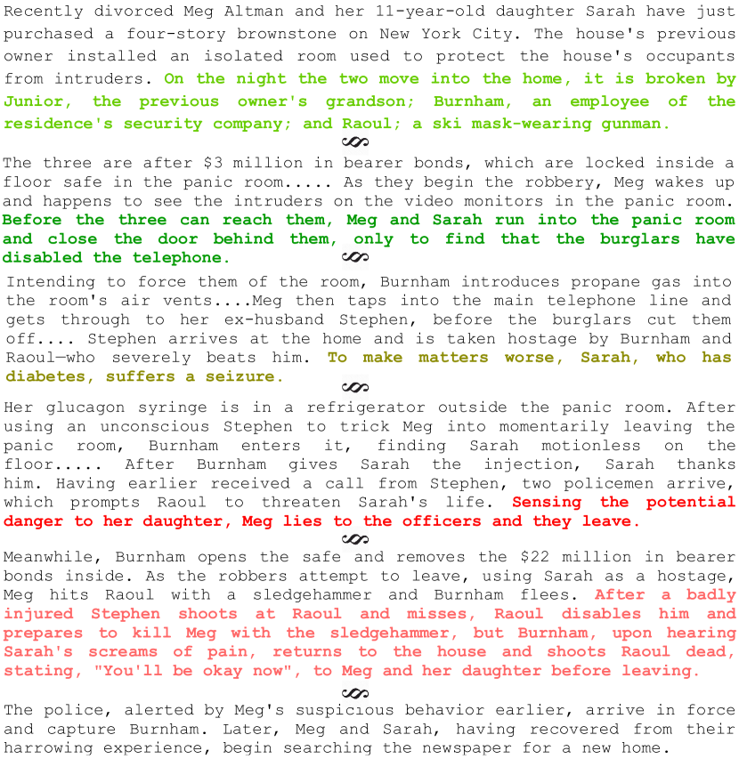
Figure 1: Example of turning point annotations (TP1, TP2, TP3, TP4, TP5, respectively) for the synopsis of the movie “Panic Room”.

We propose the task of turning point identification in movies as a means of analyzing their narrative structure. TP identification provides a sequence of key events in the story and segments the screenplay into thematic units. Common approaches to summarization and QA of long or multiple documents Chen et al. (2017); Yang et al. (2018); Kratzwald and Feuerriegel (2018); Elgohary et al. (2018) include a retrieval system as the first step, which selects a subset of relevant passages for further processing. However, Kočiskỳ et al. (2018) demonstrate that these approaches do not perform equally well for extended narratives, since individual passages are very similar and the same entities are referred to throughout the story. We argue that this challenge can be addressed by TP identification, which finds the most important events and segments the narrative into thematic units. Downstream processing for summarization or question answering can then focus on those segments that are relevant to the task.

Problematically for modeling purposes, TPs are latent in screenplays, there are no scriptwriting conventions (like character cues or scene headings) to denote where TPs occur, and their exact manifestation varies across movies (depending on genre and length), although there are some rules of thumb indicating where to expect a TP (e.g., the Opportunity occurs after the first 10% of a screenplay, Change of Plans is approximately 25% in). To enable automatic TP identification, we develop a new dataset which consists of screenplays, plot synopses, and turning point annotations. To save annotation time and render the labeling task feasible, we collect TP annotations at the plot synopsis level (synopses are a few paragraphs long compared to screenplays which are on average 120 pages long). An example is given in Figure 1. We then project the TP annotations via distant supervision onto screenplays and propose an end-to-end neural network model which identifies TPs in full length screenplays.

Our contributions can be summarized as follows: (a) we introduce TP identification as a new task for the computational analysis of screen plays that can benefit applications such as QA and summarization; (b) we create and make publicly available the TuRnIng POint Dataset (TRIPOD) which contains 99 movies (3,329 synopsis sentences and 13,403 screenplay scenes) annotated with TPs; and (c) we present an end-to-end neural network model that identifies turning points in plot synopses and projects them onto scenes in screenplays, outperforming strong baselines based on state-of-the-art sentence representations and the expected position of TPs.

2 Related Work

Recent years have seen increased interest in the automatic analysis of long and complex narratives. Specifically, Machine Reading Comprehension (MRC) and Question Answering (QA) tasks are transitioning from investigating single short and clean articles or queries Rajpurkar et al. (2016); Nguyen et al. (2016); Trischler et al. (2016) to large scale datasets that consist of complex stories Tapaswi et al. (2016); Frermann et al. (2018); Kočiskỳ et al. (2018); Joshi et al. (2017) or require reasoning across multiple documents Welbl et al. (2018); Wang et al. (2018); Dua et al. (2019); Yang et al. (2018). Tapaswi et al. (2016) introduce a multi-modal dataset consisting of questions over 140 movies, while Frermann et al. (2018) attempt to answer a single question, namely who is the perpetrator in 39 episodes of the well-known crime series CSI, again based on multi-modal information. Finally, Kočiskỳ et al. (2018) recently introduced a dataset consisting of question-answer pairs over 1,572 movie screenplays and books.

Previous approaches have focused on fine-grained story analysis, such as inducing character types Bamman et al. (2013, 2014) or understanding relationships between characters Iyyer et al. (2016); Chaturvedi et al. (2017). Various approaches have also attempted to analyze the goal and structure of narratives. Black and Wilensky (1979) evaluate the functionality of story grammars in story understanding, Elson and McKeown (2009) develop a platform for representing and reasoning over narratives, and Chambers and Jurafsky (2009) learn fine-grained chains of events.

In the context of movie summarization, Gorinski and Lapata (2018) automatically generate an overview of the movie’s genre, mood, and artistic style based on screenplay analysis. Gorinski and Lapata (2015) summarize full length screenplays by extracting an optimal chain of scenes via a graph-based approach centered around the characters of the movie. A similar approach has also been adopted by Vicol et al. (2018), who introduce the MovieGraphs dataset consisting of 51 movies and describe video clips with character-centered graphs. Other work creates animated story-boards using the action descriptions of screenplays Ye and Baldwin (2008), extracts social networks from screenplays Agarwal et al. (2014a), or creates xkcd movie narrative charts Agarwal et al. (2014b).

Our work also aims to analyze the narrative structure of movies, but we adopt a high-level approach. We advocate TP identification as a precursor to more fine-grained analysis that unveils character attributes and their relationships. Our approach identifies key narrative events and segments the screenplay accordingly; we argue that this type of preprocessing is useful for applications which might perform question answering and summarization over screenplays. Although our experiments focus solely on the textual modality, turning point analysis is also relevant for multimodal tasks such as trailer generation and video summarization.

3 The TRIPOD Dataset

The TRIPOD dataset contains 99 screenplays, accompanied with cast information (according to IMDb), and Wikipedia plot synopses annotated with turning points. The movies were selected from the Scriptbase dataset Gorinski and Lapata (2015) based on the following criteria: (a) maintaining a variation across different movie genres (e.g., action, romance, comedy, drama) and narrative types (e.g., flashbacks, time shifts); and (b) including screenplays that are faithful to the released movies and their synopses as much as possible. In Table 2, we present various statistics of the dataset.

Our motivation for obtaining TP annotations at the synopsis level (coarse-grained), instead of at the screenplay level (fine-grained) was twofold. Firstly, on account of being relatively short, synopses are easier to annotate than full-length screenplays, allowing us to scale the dataset in the future. Secondly, we would expect synopsis-level annotations to be more reliable and the degree of inter-annotator agreement higher; asking annotators to identify precisely where a turning point occurs might seem like looking for a needle in a haystack. An example of a synopsis with TP annotations is shown in Figure 1 for the movie “Panic Room”. Each TP is colored differently, and both the chain of key events (colored text) and resulting segmentation ( § ) are illustrated.

	Train	Test
movies	84	15
turning points	420	75
synopsis sentences	2,821	508
screenplay scenes	11,320	2,083
synopsis vocabulary	7.9k	2.8k
screenplay vocabulary	37.8k	16.8k
per synopsis
tokens	729.8 (165.5)	698.4 (187.4)
sentences	35.4 (8.4)	33.9 (9.9)
sentence tokens	20.6 (9.5)	20.6 (9.3)
per screenplay
tokens	23.0k (6.6)	20.9k (4.5)
sentences	3.0k (0.9)	2.8k (0.6)
scenes	133.0 (61.1)	138.9 (50.7)
per scene
tokens	173.0 (235.0)	150.5 (198.3)
sentences	22.2 (31.5)	19.9 (26.9)
sentence tokens	7.8 (6.0)	7.6 (6.4)

Table 2: Statistics of the TRIPOD dataset; all means are shown with standard deviation in brackets.

In an initial pilot study, the three authors acted as annotators for identifying TPs in movie synopses. They selected exactly one sentence per TP, under the assumption that all TPs are present. Based on the pilot, annotation instructions were devised and an annotation tool was created which allows to label synopses with TPs sentence-by-sentence. After piloting the annotation scheme on 30 movies, two new annotators were trained using our instructions and in a second study, they doubly annotated five movies. The remaining movies in the dataset were then single annotated by the new annotators.

We computed inter-annotator agreement using two different metrics: (a) total agreement (TA), i.e., the percentage of TPs that two annotators agree upon by selecting the exact same sentence; and (b) annotation distance, i.e., the distance $d[p_{i},tp_{i}]$ between two annotations for a given TP, normalized by synopsis length:

$$d[p_{i},tp_{i}]=\frac{1}{N}|p_{i}-tp_{i}|$$ (1)

where $N$ is the number of synopsis sentences and $tp_{i}$ and $p_{i}$ are the indices of the sentences labeled with TP $i$ by two annotators. The mean annotation distance $D$ is then computed by averaging distances $d[p_{i},tp_{i}]$ across all annotated TPs.

The TA between the two annotators in our second study was 64.00% and the mean annotation distance was 4.30% (StDev 3.43%). The annotation distance per TP is presented in Table 5 (last line), where it is compared with the automatic TP identification results (to be explained later).

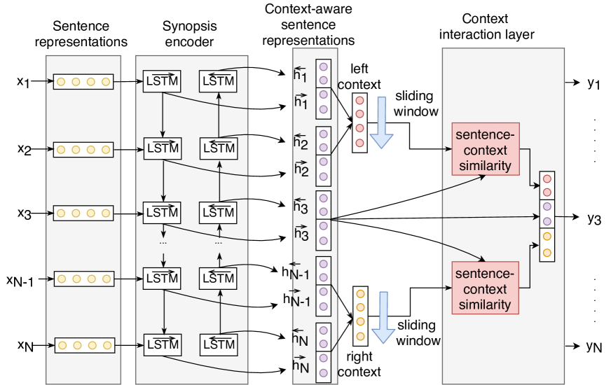
(a) Topic-Aware Model (TAM)

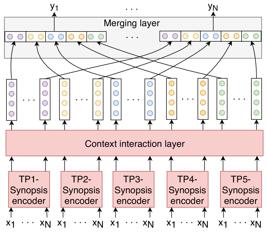
(b) Multi-view TAM

Figure 2: Model overview for TP identification in synopses. On the left, sentence representations $x_{i}$ are contextualized via a synopsis encoder (BiLSTM layer) and after interacting with the left and right windows in the context interaction layer, the final sentence representation $y_{i}$ is computed. On the right, five different synopsis encoders are utilized, one per TP, and these different views of a synopsis sentence $x_{i}$ are combined in the merging layer.

We also asked our annotators to annotate the screenplays (rather than synopses) for a subset of 15 movies. This subset serves as our goldstandard test set. Annotators were given synopses annotated with TPs and were instructed to indicate for each TP which scenes in the screenplay correspond to it. Six of the 15 movies were doubly annotated, so that we could measure agreement. Since annotators were allowed to choose a variable number of scenes for each TP, this changes slightly our agreement metrics.

Total Agreement (TA) now is the percentage of TP scenes the annotators agree on:

$$TA=\frac{1}{T\cdot L}\sum_{i=1}^{T\cdot L}{\frac{|S_{i}\cap G_{i}|}{|S_{i}\cup G_{i}|}}$$ (2)

where $T$, $L$ are the TPs identified per annotator in a screenplay, and $S_{i}$ and $G_{i}$ are the indices of the scenes selected for TP $i$ by the two annotators. Partial Agreement (PA) is the percentage of TPs where there is an overlap of at least one scene:

$$PA=\frac{1}{T\cdot L}\sum_{i=1}^{T\cdot L}{\left[S_{i}\cap G_{i}\neq\emptyset\right]}$$ (3)

And annotation distance $D$ becomes the mean of the distances $d[S_{i},G_{i}]$ between two annotators normalized by $M$, the length of the screenplay:

$$d[S_{i},G_{i}]=\frac{1}{M}\min_{(s\in S_{i},g\in G_{i})}|s-g|$$ (4)

The TA and PA between the two annotators were 35.48% and 56.67%, respectively. The mean annotation distance was 1.48% (StDev 2.93%). The TA shows that the annotators rarely indicate the same scenes, even if they are asked to annotate an event in the screenplay that is described by a specific synopsis sentence. However, they identify scenes which are in close proximity in the screenplay, as PA and annotation distance reveal. This analysis validates our assumption that annotating the synopses first limits the degree of overall disagreement.

4 Turning Point Prediction Models

In this work, we aim to detect text segments which act as TPs. We first identify which sentences in plot synopses are TPs (Section 4.1); next, we identify which scenes in screenplays act as TPs via projection of goldstandard TP labels (Section 4.2); finally, we build an end-to-end system which identifies TPs in screenplays based on predicted TP synopsis labels (Section 4.3).

All models we propose in this paper have the same basic structure; they take text segments $i$ (sentences or scenes) as input and predict whether these act as TPs or not. Since the sequence, number, and labels of TPs are fixed (see Table 1), we treat TP identification as a binary classification problem (where 1 indicates that the text is a TP and 0 otherwise). Each segment is encoded into a multi-dimensional feature space $x_{i}$ which serves as input to a fully-connected layer with a single neuron representing the probability that $i$ acts as a TP. In the following, we describe several models which vary in the way input segments are encoded.

4.1 Identifying Turning Points in Synopses

Context-Aware Model (CAM)

A simple baseline model would compute the semantic representation of each sentence in the synopsis using a pre-trained sentence encoder. However, classifying segments in isolation without considering the context in which they appear, might yield inferior semantic representations. We therefore obtain richer representations for sentences by modeling their surrounding context. We encode the synopsis with a Bidirectional Long Short-Term Memory (BiLSTM; Hochreiter and Schmidhuber 1997) network; and obtain contextualized representation $cp_{i}$ for sentence $x_{i}$ by concatenating the hidden layers of the forward $\overrightarrow{h_{i}}$ and backward $\overleftarrow{h_{i}}$ LSTM, respectively: $cp_{i}=h_{i}=[\overrightarrow{h_{i}};\overleftarrow{h_{i}}]$ (for a more detailed description, see the Appendix). Representation $cp_{i}$ is the input feature vector for our binary classifier. The model is illustrated in Figure 2(a).

Topic-Aware Model (TAM)

TPs by definition act as boundaries between different thematic units in a movie. Furthermore, long documents are usually comprised of topically coherent text segments, each of which contains a number of text passages such as sentences or paragraphs Salton et al. (1996). Inspired by text segmentation approaches Hearst (1997) which measure the semantic similarity between sequential context windows in order to determine topic boundaries, we enhance our representations with a context interaction layer. The objective of this layer is to measure the similarity of the current sentence with its preceding and following context, thereby encoding whether it functions as a boundary between thematic sections. The enriched model with the context interaction layer is illustrated in Figure 2(a).

After calculating contextualized sentence representations $cp_{i}$, we compute the representation of the left $lc_{i}$ and right $rc_{i}$ contexts of sentence $i$ (see Figure 2(a), right-hand side). We select windows of fixed length $l$ and calculate $lc_{i}$ and $rc_{i}$ by averaging the sentence representations within each window. Next, we compute the semantic similarity of the current sentence with each context representation. Specifically, we consider the element-wise product $b_{i}$, cosine similarity $c_{i}$ and pairwise distance $u_{i}$ as similarity metrics:

$$b_{i}=cp_{i}\odot lc_{i}\quad\quad c_{i}=\frac{cp_{i}\cdot lc_{i}}{\mathinner{\!\left\lVert cp_{i}\right\rVert}\mathinner{\!\left\lVert lc_{i}\right\rVert}}$$ (5)

$$u_{i}=\dfrac{cp_{i}\cdot lc_{i}}{\max(\|cp_{i}\|_{2}\cdot\|lc_{i}\|_{2})}$$ (6)

The interaction representation of sentence $cp_{i}$ with its left context is the concatenation of $cp_{i}$, $fl_{i}$, and the above similarity values (i.e., $b_{i},c_{i},u_{i}$):

$$fl_{i}=[cp_{i};lc_{i};b_{i};c_{i};u_{i}]$$ (7)

The interaction representation $fr_{i}$ for the right context $rc_{i}$ is computed analogously. We obtain the final representation of sentence $i$ via concatenating $fl_{i}$ and $fr_{i}$: $y_{i}=[fl_{i};fr_{i};cp_{i}]$.

TP-Specific Information

Another variation of our model is to use TP-specific encoders instead of a single one (see Figure 2(b)). In this case, we employ five different encoders for calculating five different representations for the current synopsis sentence $x_{i}$, each one with respect to a specific TP. These representations can be considered multiple views of the same sentence. We calculate the interaction of each view with the left and right context window, as previously, via the context interaction layer. Finally we compute the sentence representation $y_{i}$ by concatenating its individual context-enriched TP representations.

Entity-Specific Information

We also enrich our model with information about entities. We first apply co-reference resolution to the plot synopses using the Stanford CoreNLP toolkit Manning et al. (2014) and substitute mentions of named entities whenever these are included in the IMDb cast list. We then obtain entity-specific sentence representations as follows. Our encoder uses a word embedding layer initialized with pre-trained entity embeddings and a BiLSTM for contextualizing word representations. We add an attention mechanism on top of the LSTM, which assigns a weight to each word representation. We compute the entity-specific representation $e_{i}$ for synopsis sentence $i$ as the weighted sum of its word representations (for more details, see the Appendix). Finally, entity enriched sentence representations $x_{i}^{\prime}$ are obtained by concatenating generic vectors $x_{i}$ with entity-specific ones $e_{i}$: $x_{i}^{\prime}=[x_{i};e_{i}]$.

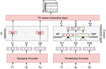
Figure 3: TAM overview for TP identification in screenplays. The synopsis and screenplay encoders contextualize synopsis sentences $x_{i}$ and screenplay scenes $s_{i}$, respectively. TPs are selected from contextualized synopsis sentences $y_{i}$ and a richer representation $sc_{i}$ is computed for $s_{i}$ via the context interaction layer. The similarity between sentence $tp_{i}$ and scene $z_{i}$ is computed by the TP–scene interaction layer.

4.2 Identifying Turning Points in Screenplays

Identifying TPs in synopses serves as a testbed for validating some of the assumptions put forward in this work, namely that turning points mark narrative progression and can be identified automatically based on their lexical makeup. Nevertheless, we are mainly interested in the real-world scenario where TPs are detected in longer documents such as screenplays. Screenplays are naturally segmented into scenes, which often describe a self-contained event that takes place in one location, and revolves around a few characters. We therefore assume that scenes are suitable textual segments for signaling TPs in screenplays.

Unfortunately, we do not have any goldstandard information about TPs in screenplays. We provide distant supervision by constructing noisy labels based on goldstandard TP annotations in synopses (see the description below). Given sentences labeled as TPs in a synopsis, we identify scenes in the corresponding screenplay which are semantically similar to them. We formulate this task as a binary classification problem, where a sentence-scene pair is deemed either “relevant” or “irrelevant” for a given TP.

Distant Supervision

Based on the screenwriting scheme of Hague (2017), TPs are expected to occur in specific parts of a screenplay (e.g., the Climax is likely to occur towards the end). We exploit this knowledge as a form of distant supervision. We estimate the mean position for each TP using the gold standard annotation of the plot synopses in our training set (normalized by the synopsis length). The results are shown in Table 3, together with the TP positions postulated by screenwriting theory. We observe that our estimates agree well with the theoretical predictions, but also that some TPs (e.g., TP2 and TP3) are more variable in their position than others (e.g., TP1 and TP5). This leads us to the following hypothesis: each TP is situated within a specific window in a screenplay. Scenes that lie within the window are semantically related to the TP, whereas all other scenes are unrelated. In experiments we calculate a window $\mu\pm\sigma$ based on our data (see Table 3).

	TP1	TP2	TP3	TP4	TP5
theory	10.00	25.00	50.00	75.00	94.50
$\mu$	11.39	31.86	50.65	74.15	89.43
$\sigma$	6.72	11.26	12.15	8.40	4.74

Table 3: Expected TP position based on screenwriting theory; mean position $\mu$ and standard deviation $\sigma$ in goldstandard synopses of our training set.

We compute scene representations based on the sequence of sentences that comprise it using a BiLSTM equipped with an attention mechanism (see Section 4.1). The final scene representation $s$ is the weighted sum of the representations of the scene sentences. Next, the TP–scene interaction layer enriches scene representations with similarity values with each marked TP synopsis sentence $tp$ as shown in Equations (5)–(7).

We again augment the above-described base model with contextualized sentence and scene representations using a synopsis and screenplay encoder. The synopsis encoder is the same one used for our sentence-level TP prediction task (see Section 4.1). The screenplay encoder works in a similar fashion over scene representations.

Topic-Aware Model (TAM)

TAM enhances our screenplay encoder with information about topic boundaries. Specifically, we compute the representations of the left $lc_{i}$ and right $rc_{i}$ context window of the $i^{th}$ scene in the screenplay as described in Section 4.1. Next, we compute the final representation $z_{i}$ of scene $sc_{i}$ by concatenating the representations of the context windows $lc_{i}$ and $rc_{i}$ and the current scene $sc_{i}$: $z_{i}=[lc_{i};sc_{i};rc_{i}]$. There is no need to compute the similarity between scenes and context windows here as we now have goldstandard TP representations in the synopsis and employ the TP–scene interaction layer for the computation of the similarity between TPs and enriched scene representations $z_{i}$. Hence, we directly calculate in this layer a scene-level feature vector that encodes information about the scene, its similarity to TP sentences, and whether these function as boundaries between topics in the screenplay.

Entity-Specific information

We can also employ an entity-specific encoder (see Section 4.1) for the representing the synopsis and scene sentences. Again, generic and entity-specific representations are combined via concatenation.

4.3 End-to-end TP Identification

Our ultimate goal is to identify TPs in screenplays without assuming any goldstandard information about their position in the synopsis. We address this with an end-to-end model which first predicts the sentences that act as TPs in the synopsis (e.g., TAM in Section 4.1) and then feeds these predictions to a model which identifies the corresponding TP scenes (e.g., TAM in Section 4.2).

5 Experimental Setup

Training

We used the Universal Sentence Encoder (USE; Cer et al. 2018) as a pre-trained sentence encoder for all models and tasks; its performance was superior to BERT Devlin et al. (2018) and other related pre-trained encoders (for more details, see the Appendix). Since the binary labels in both prediction tasks are imbalanced, we apply class weights to the loss function of our models. We weight each class by its inverse frequency in the training set (for more implementation details, see the Appendix).

Inference

During inference in our first task (i.e., identification of TPs in synopses), we select one sentence per TP. Specifically, we want to track the five sentences with the highest posterior probability of being TPs and sequentially assign them TP labels based on their position. However, it is possible to have a cluster of neighboring sentences with high probability, even though they all belong to the same TP. We therefore constrain the sentence selection for each TP within the window of its expected position, as calculated in the distribution baseline (Section 4.2).

For models which predict TPs in screenplays, we obtain a probability distribution over all scenes in a screenplay indicating how relevant each is to the TPs of the corresponding plot synopsis. We find the peak of each distribution and select a neighborhood of scenes around this peak as TP-relevant ones. Based on the goldstandard annotation, each TP corresponds to 1.77 relevant scenes on average (StDev 1.23). We therefore consider a neighborhood of three relevant scenes per TP.

	$TA$	$D$
Baseline	31.00	9.65 (4.41)
CAM	33.00	7.44 (8.09)
TAM	36.00	7.11 (7.98)
+ TP views	39.00	6.52 (7.72)
+ entities	38.00	6.91 (7.65)

(a) Development set

	$TA$	$D$
Random	2.00	37.79 (25.33)
Theory baseline	22.00	7.47 (6.75)
Distribution baseline	28.00	7.28 (6.23)
TAM	34.67	6.80 (5.19)
+ TP views	38.57	7.47 (7.48)
+ entities	41.33	7.30 (7.21)
Human agreement	64.00	4.30 (3.43)

(b) Test set

Table 4: Identification of TPs in plot synopses; results are shown in percent ($TA$: mean Total Agreement; $D$: annotation distance; standard deviation in brackets).

TAM	TP1	TP2	TP3	TP4	TP5
+ TP views	6.09	9.45	10.72	6.91	4.26
+ entities	7.18	9.35	9.86	5.23	3.48
Human agreement	3.33	5.00	10.58	1.07	1.53

Table 5: Mean annotation distance $D$ (test set); results are shown per TP on the synopsis identification task.

6 Results

TP Identification in Synopses Table 4(a) reports our results on the development set (we extracted 20 movies from the original training set) which aim at comparing various model instantiations for the TP identification task. Specifically, we report the performance of a baseline model which is neither context-aware nor utilizes topic boundary information against CAM and TAM. We also show two variants of TAM enhanced with TP-specific encoders (+ TP views) and entity-specific information (+ entities). Model performance is measured using the evaluation metrics of Total Agreement ($TA$) and annotation distance ($D$), normalized by synopsis length (equation (1)).

The baseline model presents the lowest performance among all variants which suggests that state-of-the-art sentence representations on their own are not suitable for our task. Indeed, when contextualizing the synopsis sentences via a BiLSTM layer we observe an absolute increase of 4.00% in terms of $TA$. Moreover, the addition of a context interaction layer (see TAM row in Table 4(a)) yields an absolute $TA$ improvement of 4.00% compared to CAM. Combining different TP views further improves by 3.00%, reaching a $TA$ of 39.00%, and reducing $D$ to 6.52%.

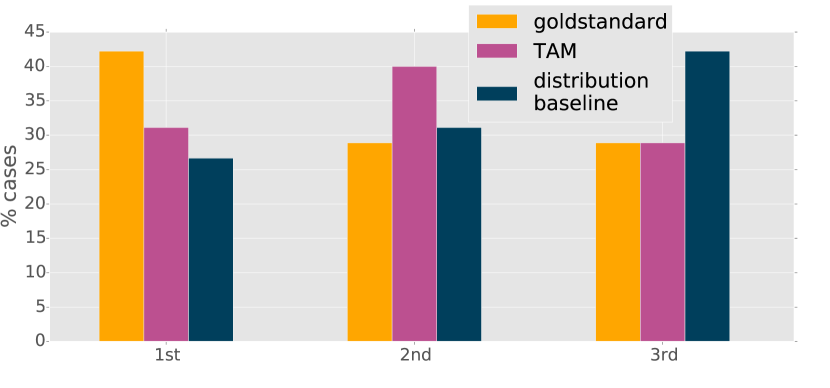
Figure 4: Rankings (shown as proportions) of synopsis highlights produced by aggregating goldstandard TP annotations, those predicted by the distribution baseline, and our model (TAM + TP views).

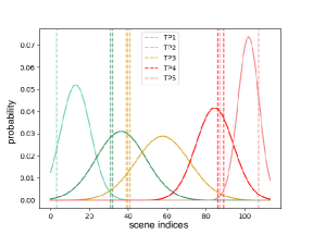
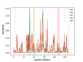
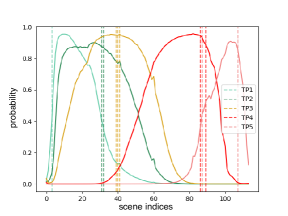
Distribution baseline	tf*idf similarity	TAM

Figure 5: Probability distributions over the scenes of the screenplay for the movie “Juno”; x-axis: scene indices, y-axis: probability that the scene is relevant to a specific TP. Vertical dashed lines are goldstandard TP scenes.

Table 4(b) shows our results on the test set. We compare TAM, our best performing model against two strong baselines. The first one selects sentences that lie on the expected positions of TPs according to screenwriting theory; while the second one selects sentences that lie on the peaks of the empirical TP distributions in the training set (Section 4.2). As we can see, TAM (+ TP views) achieves a $TA$ of 38.57% compared to 22.00% for the distribution baseline. And although entity-specific information does not have much impact on the development set, it yields a 2.76% improvement on the test set. A detailed break down of results per TP is given in Table 5. Interestingly, our model resembles human behavior (see row Human agreement): TPs 1, 4, and 5 are easiest to distinguish, whereas TPs 2 and 3 are hardest and frequently placed at different points in the synopsis.

We also conducted a human evaluation experiment on Amazon Mechanical Turk (AMT). AMT workers were presented with a synopsis and “highlights”, i.e., five sentences corresponding to TPs. We obtained highlights from goldstandard annotations, the distribution baseline, and TAM (+ TP views). AMT workers were asked to read the synopsis and rank the highlights from best to worst according to the following criteria: (1) the quality of the plotline that they form; (2) whether they include the most important events and plot twists of the movie; and (3) whether they provide some description of the events in the beginning and end of the movie. In Figure 4 we show, proportionally, how often our participants ranked each model 1st, 2nd, and so on. Perhaps unsurprisingly, goldstandard TPs were considered best (and ranked 1st 42% of the time). TAM is ranked best 30% of the time, followed by the distribution baseline which was only ranked first 26% of the time. Overall, the average ranking positions for the goldstandard, TAM, and the baseline are 1.87, 1.98, and 2.16, respectively. Human evaluation therefore validates that our model outperforms the position-based baselines.

	$TA$	$PA$	$D$
Theory baseline	8.66	10.67	10.45 (9.14)
Distribution baseline	6.67	9.33	10.84 (8.94)
tf*idf similarity	0.74	1.33	53.07 (31.83)
tf*idf + distribution	4.44	6.67	13.33 (11.51)
CAM	11.11	16.00	10.23 (11.23)
+ entities	14.18	17.33	12.77 (12.61)
TAM	10.63	13.33	8.94 (9.39)
+ entities	10.63	13.33	10.15 (10.56)
TAM End2end	7.87	9.33	10.16 (10.74)
Human agreement	35.48	56.67	1.48 (2.93)

Table 6: Identification of TPs in screenplays; results are shown in percent using five-fold cross validation ($TA$: mean Total Agreement; $PA$: Partial Agreement; $D$: annotation distance $D$; standard deviation in brackets).

TP Identification in Screenplays

Our results are summarized in Table 6. For this task, we performed five-fold crossvalidation over our original goldstandard set to obtain a test-development split (recall we do not have goldstandard annotations for training). We report Total Agreement ($TA$), Partial Agreement ($PA$), and annotation distance $D$, normalized by screenplay length (Equations (2)–(4)).

Aside from the theory and distribution-based baselines, we also experimented with a common IR baseline which considers TP synopsis sentences as queries and retrieves a neighborhood of semantically similar scenes from the screenplay using tf*idf similarity. Specifically, we compute the maximum tf*idf similarity for all sentences included in the respective scene. We empirically observed that tf*idf’s behavior can be erratic selecting scenes in completely different sections of the screenplay, and therefore constrain it by selecting scenes only within the windows determined by the position distributions ($\mu\pm\sigma$) for each TP. As far as our own models are concerned, we report results with goldstandard TP labels for CAM and TAM on their own and enriched with entity information. We also built and end-to-end system based on TP predictions from TAM.

As can be seen in Table 6, tf*idf approaches perform worse than position-related baselines. Overall, similar vocabulary across scenes and mentions of the same entities throughout the screenplay make tf*idf approaches insufficient for our tasks. The best performing model is TAM confirming our hypothesis that TPs are not just isolated key events, but also mark boundaries between thematic units and, therefore, segmentation-inspired approaches can be beneficial for the task. Results for entities are somewhat mixed; for CAM, the entity-specific information improves $TA$ and $PA$ but increases $D$, while it does not seem to make much difference for TAM. The performance of the end-to-end TAM model drops slightly compared to the same model using goldstandard TP annotations. However, it still remains competitive against the baselines, indicating that tracking TPs in screenplays fully automatically is feasible.

In Figure 5, we visualize the posterior distribution of various models over the scenes of the screenplay for the movie “Juno”. The first panel shows the distribution baseline alongside goldstandard TP scenes (vertical lines). We observe that the distribution baseline provides a good approximation of relevant TP positions (which validates its use in the construction of noisy labels, Section 4.2), even though it is not always accurate. For example, TPs 1 and 3 lie outside the expected window in “Juno”.

The second panel presents the TP predictions according to tf*idf similarity. We observe that scenes located in entirely different parts of the screenplay present high similarity scores with respect to a given TP due to vocabulary uniformity and mentions of the same entities throughout the screenplay. In the next panel we present the predictions of TAM. Adding synopsis and screenplay encoders yields smoother distributions increasing the probability of selecting TP scenes inside distinct regions of the screenplay, with sharper peaks and higher confidence.

7 Conclusions

We proposed the task of turning point identification in screenplays as a means of analyzing their narrative structure. We demonstrated that automatically identifying a sequence of key events and segmenting the screenplay into thematic units is feasible via an end-to-end neural network model. In future work, we will investigate the usefulness of TPs for summarization and question answering. We will also scale the TRIPOD dataset and move to a multi-modal setting where TPs are identified directly in video data.

Appendix A Model Details

Synopsis Encoder

In all tasks we use a synopsis encoder in order to contextualize the sentences in the synopsis. We employ an LSTM network as the synopsis encoder which produces sentence representations $h_{1},h_{2},\dots,h_{T}$, where $h_{i}$ is the hidden state at time-step $i$, summarizing all the information of the synopsis up to the $i$-th sentence. We use a Bidirectional LSTM (BiLSTM) in order to get sentence representations that summarize the information from both directions. A BiLSTM consists of a forward LSTM $\overrightarrow{f}$ that reads the synopsis from $p_{1}$ to $p_{N}$ and a backward LSTM $\overleftarrow{f}$ that reads it from $p_{N}$ to $p_{1}$. We obtain the final representation $cp_{i}$ for a given synopsis sentence $p_{i}$ by concatenating the representations from both directions, $cp_{i}=h_{i}=[\overrightarrow{h_{i}};\overleftarrow{h_{i}}],\quad h_{i}\in R^{2S},$ where $S$ denotes the size of each LSTM.

Entity-Specific Encoder

This encoder is used to evaluate the contribution of entity-specific information to the performance of our models. We use a word embedding layer to project words $w_{1},w_{2},\dots,w_{T}$ of the $i^{th}$ synopsis sentence $p_{i}$ to a continuous vector space $R^{E}$, where $E$ the size of the embedding layer. This layer is initialized with pre-trained entity embeddings. Next, we use a BiLSTM as described in the case of the synopsis encoder. On top of the LSTM, we add an attention mechanism, which assigns a weight $a_{i}$ to each word representation $h_{i}$. We compute the entity-specific representation $pe_{i}$ of the $i^{th}$ plot sentence as the weighted sum of word representations:

$$e_{j}=\tanh(W_{h}h_{j}+b_{h}),\quad e_{j}\in[-1,1]$$ (8)

$$a_{j}=\dfrac{\exp(e_{j})}{\sum_{t=1}^{T}\exp(e_{t})},\quad\sum_{j=1}^{T}a_{j}=1$$ (9)

$$pe_{i}=\sum_{j=1}^{T}a_{j}h_{j},\quad e\in R^{2S}$$ (10)

where $W_{h}$ and $b_{h}$ are the attention layer’s weights.

Goldstandard

• Sixteen-year-old Minnesota high-schooler Juno MacGuff discovers she is pregnant with a child fathered by her friend and longtime admirer, Paulie Bleeker.

•  All of this decides her against abortion, and she decides to give the baby up for adoption.

•  With Mac, Juno meets the couple, Mark and Vanessa Loring (Jason Bateman and Jennifer Garner), in their expensive home and agrees to a closed adoption.

•  Juno watches the Loring marriage fall apart, then drives away and breaks down in tears by the side of the road.

•  Vanessa comes to the hospital where she joyfully claims the newborn boy as a single adoptive mother.

TAM (+ TP views)

• Going to a local clinic run by a women’s group, she encounters outside a school mate who is holding a rather pathetic one-person Pro-Life vigil.

•  With Mac, Juno meets the couple, Mark and Vanessa Loring (Jason Bateman and Jennifer Garner), in their expensive home and agrees to a closed adoption.

•  Juno and Leah happen to see Vanessa in a shopping mall being completely at ease with a child, and Juno encourages Vanessa to talk to her baby in the womb, where it obligingly kicks for her.

•  Juno watches the Loring marriage fall apart, then drives away and breaks down in tears by the side of the road.

•  The film ends in the summertime with Juno and Paulie playing guitar and singing together, followed by a kiss.

Distribution baseline

• Once inside, however, Juno is alienated by the clinic staff’s authoritarian and bureaucratic attitudes.

•  Juno visits Mark a few times, with whom she shares tastes in punk rock and horror films.

•  Not long before her baby is due, Juno is again visiting Mark when their interaction becomes emotional.

•  Juno then tells Paulie she loves him, and Paulie’s actions make it clear her feelings are very much reciprocated.

•  Vanessa comes to the hospital where she joyfully claims the newborn boy as a single adoptive mother.

Table 7: Highlights for the movie ”Juno”: goldstandard annotations and predicted TPs for TAM (+ TP views) and distribution baseline.

Appendix B Implementation Details

Pre-trained Sentence Encoder

The performance of our models depends on the initial sentence representations. We experimented with using the large BERT model Devlin et al. (2018) and the Universal Sentence Encoder (USE) Cer et al. (2018) as pre-trained sentence encoders in all tasks. Intuitively, we expect USE to be more suitable, since it was trained in textual similarity tasks which are more relevant to ours. Experiments on the development set confirmed our intuition. Specifically, on the screenplay TP prediction task, annotation distance $D$ dropped from 17.00% to 10.04% when employing USE instead of the BERT embeddings in the CAM version of our architecture.

Hyper-parameters

We used the Adam algorithm Kingma and Ba (2014) for optimizing our networks. After experimentation, we chose an LSTM with 32 neurons (64 for the BiLSTM) for the synopsis encoder in the first task and one with 64 neurons for the encoder in the second task. For the context interaction layer, the window $l$ was set to two sentences for the first task and 20% of the screenplay length for the second task. For the entity encoder, an embedding layer of size 300 was initialized with the Wikipedia2Vec pre-trained word embeddings Yamada et al. (2018) and remained frozen during training. The LSTM of the encoder had 32 and 64 neurons for the first and second tasks, respectively. Finally, we also added a dropout of 0.2. For developing our models we used PyTorch Paszke et al. (2017).

Data Augmentation

We used multiple annotations for training for movies where these were available and considered reliable. The reasons for this are twofold. Firstly, this allowed us to take into account the subjective nature of the task during training; and secondly, it increased the size of our dataset, which contains a limited number of movies. Specifically, we added triplicate annotations for 17 movies and duplicate annotations for 5 movies.

Goldstandard

• On the night the two move into the home, it is broken into by Junior, the previous owner’s grandson; Burnham, an employee of the residence’s security company; and Raoul, a ski mask-wearing gunman recruited by Junior.

•  Before the three can reach them, Meg and Sarah run into the panic room and close the door behind them, only to find that the burglars have disabled the telephone.

•  To make matters worse, Sarah, who has diabetes, suffers a seizure.

•  Sensing the potential danger to her daughter, Meg lies to the officers and they leave.

•  After a badly injured Stephen shoots at Raoul and misses, Raoul disables him and prepares to kill Meg with the sledgehammer, but Burnham, upon hearing Sarah’s screams of pain, returns to the house and shoots Raoul dead, stating, ”You’ll be okay now”, to Meg and her daughter before leaving.

TAM (+ TP views)

• On the night the two move into the home, it is broken into by Junior, the previous owner’s grandson; Burnham, an employee of the residence’s security company; and Raoul, a ski mask-wearing gunman recruited by Junior.

•  Before the three can reach them, Meg and Sarah run into the panic room and close the door behind them, only to find that the burglars have disabled the telephone.

•  Her emergency glucagon syringe is in a refrigerator outside the panic room.

•  As Meg throws the syringe into the panic room, Burnham frantically locks himself, Raoul, and Sarah inside, crushing Raoul’s hand in the sliding steel door.

•  After a badly injured Stephen shoots at Raoul and misses, Raoul disables him and prepares to kill Meg with the sledgehammer, but Burnham, upon hearing Sarah’s screams of pain, returns to the house and shoots Raoul dead, stating, ”You’ll be okay now”, to Meg and her daughter before leaving.

Distribution baseline

• On the night the two move into the home, it is broken into by Junior, the previous owner’s grandson; Burnham, an employee of the residence’s security company; and Raoul, a ski mask-wearing gunman recruited by Junior.

•  Unable to seal the vents, Meg ignites the gas while she and Sarah cover themselves with fireproof blankets, causing an explosion which vents into the room outside and causes a fire, injuring Junior.

•  To make matters worse, Sarah, who has diabetes, suffers a seizure.

•  While doing so, he tells Sarah he did not want this, and the only reason he agreed to participate was to give his own child a better life.

•  As the robbers attempt to leave, using Sarah as a hostage, Meg hits Raoul with a sledgehammer and Burnham flees.

Table 8: Highlights for the movie ”Panic Room”: goldstandard annotations and the predicted TPs for TAM (+ TP views) and distribution baseline.

Goldstandard

• Manager Stuart Ullman warns him that a previous caretaker developed cabin fever and killed his family and himself.

•  Hallorann tells Danny that the hotel itself has a ”shine” to it along with many memories, not all of which are good.

•  After she awakens him, he says he dreamed that he had killed her and Danny.

•  Jack begins to chop through the door leading to his family’s living quarters with a fire axe.

•  Wendy and Danny escape in Hallorann’s snowcat, while Jack freezes to death in the hedge maze.

TAM (+TP views)

• Jack’s wife, Wendy, tells a visiting doctor that Danny has an imaginary friend named Tony, and that Jack has given up drinking because he had hurt Danny’s arm following a binge.

•  Hallorann tells Danny that the hotel itself has a ”shine” to it along with many memories, not all of which are good.

•  Danny starts calling out ”redrum” frantically and goes into a trance, now referring to himself as ”Tony”.

•  When Wendy sees this in the bedroom mirror, the letters spell out ”MURDER”.

•  Wendy and Danny escape in Hallorann’s snowcat, while Jack freezes to death in the hedge maze.

Distribution baseline

• Jack’s wife, Wendy, tells a visiting doctor that Danny has an imaginary friend named Tony, and that Jack has given up drinking because he had hurt Danny’s arm following a binge.

•  Jack, increasingly frustrated, starts acting strangely and becomes prone to violent outbursts.

•  Jack investigates Room 237, where he encounters the ghost of a dead woman, but tells Wendy he saw nothing.

•  When Wendy sees this in the bedroom mirror, the letters spell out ”MURDER”.

•  He kills Hallorann in the lobby and pursues Danny into the hedge maze.

Table 9: Highlights for the movie ”The Shining”: goldstandard annotations and the predicted TPs TAM (+ TP views) and distribution baseline.

Appendix C Example Output: TP Identification in Synopses

As mentioned in Section 6, we also conducted a human evaluation experiment, where highlights were extracted by combining the five sentences labeled as TPs the synopsis. In Tables 7, 8, and 9, we present the highlights presented to the AMT workers for the movies ”Juno”, ”Panic Room”, and ”The Shining”, respectively. For each movie we show the goldstandard annotations alongside with the predicted TPs for TAM (+ TP views) and the distribution baseline, which is the strongest performing baseline with respect to the automatic evaluation results.

Overall, we observe that goldstandard highlights describe the plotline of the movie, contain a first introductory sentence, some major and intense events, and a last sentence that describes the ending of the story.

The distribution baseline is able to predict a few goldstandard TPs by only considering the relative position of the sentences in the synopsis. This observation validates the screenwriting theory: TPs, or more generally important events that determine the progression of the plot, are consistently distributed in specific parts of a movie. However, when the distribution baseline cannot predict the exact TP sentence, it might select one that describes irrelevant events of minor importance (e.g., TP4 for ”Panic Room” is a detail about a secondary character instead of a major setback and highly intense event in the movie).

Finally, our own model seems to be able to predict some goldstandard TP sentences, as demonstrated during the automatic evaluation. However, we also observe here that even when it does not select the goldstandard TPs, the predicted ones describe important events in the movie that have some desired characteristics. In particular, for the movie ”Juno” the climax (TP5) is the moment of resolution, where Vanessa decides to adopt the baby after all the setbacks and obstacles. Even though our model does not predict this sentence, it does select one that reveals information about the ending of the movie. An other such example is the movie ”Panic Room”, where the point of no return (TP3) is not correctly predicted, but the selected sentence refers to the same event.

References

- Agarwal et al. (2014a) Apoorv Agarwal, Sriramkumar Balasubramanian, Jiehan Zheng, and Sarthak Dash. 2014a. Parsing Screenplays for Extracting Social Networks from Movies. In Proceedings of the 3rd Workshop on Computational Linguistics for Literature, pages 50–58, Gothenburg, Sweden.
- Agarwal et al. (2014b) Apoorv Agarwal, Sarthak Dash, Sriramkumar Balasubramanian, and Jiehan Zheng. 2014b. Using Determinantal Point Processes for Clustering with Application to Automatically Generating and Drawing xkcd Movie Narrative Charts. In Proceedings of the 2nd Academy of Science and Engineering International Conference on Big Data Science and Computing, Stanford, California.
- Agarwal et al. (2015) Apoorv Agarwal, Jiehan Zheng, Shruti Kamath, Sriramkumar Balasubramanian, and Shirin Ann Dey. 2015. Key Female Characters in Film Have More to Talk About Besides Men: Automating the Bechdel Test. In Proceedings of the 2015 Conference of the North American Chapter of the Association for Computational Linguistics: Human Language Technologies, pages 830–840, Denver, Colorado.
- Bamman et al. (2013) David Bamman, Brendan O’Connor, and Noah A Smith. 2013. Learning latent personas of film characters. In Proceedings of the 51st Annual Meeting of the Association for Computational Linguistics (Volume 1: Long Papers), volume 1, pages 352–361, Sofia, Bulgaria.
- Bamman et al. (2014) David Bamman, Ted Underwood, and Noah A Smith. 2014. A bayesian mixed effects model of literary character. In Proceedings of the 52nd Annual Meeting of the Association for Computational Linguistics (Volume 1: Long Papers), volume 1, pages 370–379.
- Black and Wilensky (1979) John B Black and Robert Wilensky. 1979. An evaluation of story grammars. Cognitive science, 3(3):213–229.
- Cer et al. (2018) Daniel Cer, Yinfei Yang, Sheng-yi Kong, Nan Hua, Nicole Limtiaco, Rhomni St John, Noah Constant, Mario Guajardo-Cespedes, Steve Yuan, Chris Tar, et al. 2018. Universal sentence encoder. arXiv preprint arXiv:1803.11175.
- Chambers and Jurafsky (2009) Nathanael Chambers and Dan Jurafsky. 2009. Unsupervised learning of narrative schemas and their participants. In Proceedings of the Joint Conference of the 47th Annual Meeting of the ACL and the 4th International Joint Conference on Natural Language Processing of the AFNLP: Volume 2-Volume 2, pages 602–610. Association for Computational Linguistics.
- Chaturvedi et al. (2017) Snigdha Chaturvedi, Mohit Iyyer, and Hal Daume III. 2017. Unsupervised learning of evolving relationships between literary characters. In Thirty-First AAAI Conference on Artificial Intelligence.
- Chen et al. (2017) Danqi Chen, Adam Fisch, Jason Weston, and Antoine Bordes. 2017. Reading wikipedia to answer open-domain questions. arXiv preprint arXiv:1704.00051.
- Cutting (2016) James E Cutting. 2016. Narrative theory and the dynamics of popular movies. Psychonomic bulletin & review, 23(6):1713–1743.
- Danescu-Niculescu-Mizil et al. (2012) Cristian Danescu-Niculescu-Mizil, Justin Cheng andJon Kleinberg, and Lillian Lee. 2012. You had me at hello: How phrasing affects memorability. In Proceedings of the 50th Annual Meeting of the Association for Computational Linguistics: Long Papers–Volume 1, pages 892–901, ??
- Devlin et al. (2018) Jacob Devlin, Ming-Wei Chang, Kenton Lee, and Kristina Toutanova. 2018. Bert: Pre-training of deep bidirectional transformers for language understanding. arXiv preprint arXiv:1810.04805.
- Dua et al. (2019) Dheeru Dua, Yizhong Wang, Pradeep Dasigi, Gabriel Stanovsky, Sameer Singh, and Matt Gardner. 2019. Drop: A reading comprehension benchmark requiring discrete reasoning over paragraphs. arXiv preprint arXiv:1903.00161.
- Elgohary et al. (2018) Ahmed Elgohary, Chen Zhao, and Jordan Boyd-Graber. 2018. A dataset and baselines for sequential open-domain question answering. In Proceedings of the 2018 Conference on Empirical Methods in Natural Language Processing, pages 1077–1083.
- Elsner (2012) Mich Elsner. 2012. Character-based kernels for novelistic plot structure. In Proceedings of the 13th Conference of the European Chapter of the Association for Computational Linguistics, pages 634–644, Avignon, France.
- Elson and McKeown (2009) David Elson and Kathleen McKeown. 2009. Extending and evaluating a platform for story understanding. In Proceedings of the AAAI 2009 Spring Symposium on Intelligent Narrative Technologies II, page ??, ??
- Frermann et al. (2018) Lea Frermann, Shay B Cohen, and Mirella Lapata. 2018. Whodunnit? crime drama as a case for natural language understanding. Transactions of the Association of Computational Linguistics, 6:1–15.
- Freytag (1896) Gustav Freytag. 1896. Freytag’s technique of the drama: an exposition of dramatic composition and art. Scholarly Press.
- Gorinski and Lapata (2015) Philip John Gorinski and Mirella Lapata. 2015. Movie script summarization as graph-based scene extraction. In Proceedings of the 2015 Conference of the North American Chapter of the Association for Computational Linguistics: Human Language Technologies, pages 1066–1076.
- Gorinski and Lapata (2018) Philip John Gorinski and Mirella Lapata. 2018. What’s this movie about? a joint neural network architecture for movie content analysis. In Proceedings of the 2018 Conference of the North American Chapter of the Association for Computational Linguistics: Human Language Technologies, Volume 1 (Long Papers), pages 1770–1781.
- Hague (2017) Michael Hague. 2017. Storytelling Made Easy: Persuade and Transform Your Audiences, Buyers, and Clients – Simply, Quickly, and Profitably. Indie Books International.
- Hearst (1997) Marti A Hearst. 1997. Texttiling: Segmenting text into multi-paragraph subtopic passages. Computational linguistics, 23(1):33–64.
- Hochreiter and Schmidhuber (1997) Sepp Hochreiter and Jürgen Schmidhuber. 1997. Long short-term memory. Neural computation, 9(8):1735–1780.
- Iyyer et al. (2016) Mohit Iyyer, Anupam Guha, Snigdha Chaturvedi, Jordan Boyd-Graber, and Hal Daumé III. 2016. Feuding families and former friends: Unsupervised learning for dynamic fictional relationships. In Proceedings of the 2016 Conference of the North American Chapter of the Association for Computational Linguistics: Human Language Technologies, pages 1534–1544.
- Joshi et al. (2017) Mandar Joshi, Eunsol Choi, Daniel S Weld, and Luke Zettlemoyer. 2017. Triviaqa: A large scale distantly supervised challenge dataset for reading comprehension. arXiv preprint arXiv:1705.03551.
- Kingma and Ba (2014) Diederik P Kingma and Jimmy Ba. 2014. Adam: A method for stochastic optimization. arXiv preprint arXiv:1412.6980.
- Kočiskỳ et al. (2018) Tomáš Kočiskỳ, Jonathan Schwarz, Phil Blunsom, Chris Dyer, Karl Moritz Hermann, Gáabor Melis, and Edward Grefenstette. 2018. The narrativeqa reading comprehension challenge. Transactions of the Association of Computational Linguistics, 6:317–328.
- Kratzwald and Feuerriegel (2018) Bernhard Kratzwald and Stefan Feuerriegel. 2018. Adaptive document retrieval for deep question answering. arXiv preprint arXiv:1808.06528.
- Manning et al. (2014) Christopher Manning, Mihai Surdeanu, John Bauer, Jenny Finkel, Steven Bethard, and David McClosky. 2014. The stanford corenlp natural language processing toolkit. In Proceedings of 52nd annual meeting of the association for computational linguistics: system demonstrations, pages 55–60.
- Nalisnick and Baird (2013) Eric T. Nalisnick and Henry S. Baird. 2013. Character-to-character sentiment analysis in shakespeare’s plays. In Proceedings of the 51st Annual Meeting of the Association for Computational Linguistics, pages 479–483, Sofia, Bulgaria.
- Nguyen et al. (2016) Tri Nguyen, Mir Rosenberg, Xia Song, Jianfeng Gao, Saurabh Tiwary, Rangan Majumder, and Li Deng. 2016. Ms marco: A human generated machine reading comprehension dataset. arXiv preprint arXiv:1611.09268.
- Paszke et al. (2017) Adam Paszke, Sam Gross, Soumith Chintala, Gregory Chanan, Edward Yang, Zachary DeVito, Zeming Lin, Alban Desmaison, Luca Antiga, and Adam Lerer. 2017. Automatic differentiation in pytorch.
- Pavis (1998) Patrice Pavis. 1998. Dictionary of the theatre: Terms, concepts, and analysis. University of Toronto Press.
- Rajpurkar et al. (2016) Pranav Rajpurkar, Jian Zhang, Konstantin Lopyrev, and Percy Liang. 2016. Squad: 100,000+ questions for machine comprehension of text. arXiv preprint arXiv:1606.05250.
- Ramakrishna et al. (2015) Anil Ramakrishna, Nikolaos Malandrakis, Elizabeth Staruk, and Shrikanth Narayanan. 2015. A quantitative analysis of gender differences in movies using psycholinguistic normatives. In Proceedings of the 2015 Conference on Empirical Methods in Natural Language Processing., pages 1996–2001, Lisbon, Portugal.
- Salton et al. (1996) Gerard Salton, Amit Singhal, Chris Buckley, and Mandar Mitra. 1996. Automatic text decomposition using text segments and text themes. In Proceedings of the the seventh ACM conference on Hypertext, pages 53–65, Bethesda, Maryland.
- Sap et al. (2017) Maarten Sap, Marcella Cindy Prasettio, Ari Holtzman, Hannah Rashkin, and Yejin Choi. 2017. Connotation frames of power and agency in modern films. In Proceedings of the 2017 Conference on Empirical Methods in Natural Language Processing, pages 2329–2334, Copenhagen, Denmark.
- Tapaswi et al. (2016) Makarand Tapaswi, Yukun Zhu, Rainer Stiefelhagen, Antonio Torralba, Raquel Urtasun, and Sanja Fidler. 2016. Movieqa: Understanding stories in movies through question-answering. In Proceedings of the IEEE conference on computer vision and pattern recognition, pages 4631–4640.
- Thompson (1999) Kristin Thompson. 1999. Storytelling in the new Hollywood: Understanding classical narrative technique. Harvard University Press.
- Trischler et al. (2016) Adam Trischler, Tong Wang, Xingdi Yuan, Justin Harris, Alessandro Sordoni, Philip Bachman, and Kaheer Suleman. 2016. Newsqa: A machine comprehension dataset. arXiv preprint arXiv:1611.09830.
- Vicol et al. (2018) Paul Vicol, Makarand Tapaswi, Lluis Castrejon, and Sanja Fidler. 2018. Moviegraphs: Towards understanding human-centric situations from videos. In Proceedings of the IEEE Conference on Computer Vision and Pattern Recognition, pages 8581–8590.
- Wang et al. (2018) Yizhong Wang, Kai Liu, Jing Liu, Wei He, Yajuan Lyu, Hua Wu, Sujian Li, and Haifeng Wang. 2018. Multi-passage machine reading comprehension with cross-passage answer verification. arXiv preprint arXiv:1805.02220.
- Welbl et al. (2018) Johannes Welbl, Pontus Stenetorp, and Sebastian Riedel. 2018. Constructing datasets for multi-hop reading comprehension across documents. Transactions of the Association of Computational Linguistics, 6:287–302.
- Yamada et al. (2018) Ikuya Yamada, Akari Asai, Hiroyuki Shindo, Hideaki Takeda, and Yoshiyasu Takefuji. 2018. Wikipedia2vec: An optimized tool for learning embeddings of words and entities from wikipedia. arXiv preprint 1812.06280.
- Yang et al. (2018) Zhilin Yang, Peng Qi, Saizheng Zhang, Yoshua Bengio, William W Cohen, Ruslan Salakhutdinov, and Christopher D Manning. 2018. Hotpotqa: A dataset for diverse, explainable multi-hop question answering. arXiv preprint arXiv:1809.09600.
- Ye and Baldwin (2008) Patrick Ye and Timothy Baldwin. 2008. Towards Automatic Animated Storyboarding. In Proceedings of the 23rd Association for the Advancement of Artificial Intelligence Conference on Artificial Intelligence, pages 578–583, Chicago, Illinois.