Bridging the Gap for Tokenizer-Free Language Models

Abstract

Purely character-based language models (LMs) have been lagging in quality on large scale datasets, and current state-of-the-art LMs rely on word tokenization. It has been assumed that injecting the prior knowledge of a tokenizer into the model is essential to achieving competitive results. In this paper, we show that contrary to this conventional wisdom, tokenizer-free LMs with sufficient capacity can achieve competitive performance on a large scale dataset. We train a vanilla transformer network with 40 self-attention layers on the One Billion Word (lm1b) benchmark and achieve a new state of the art for tokenizer-free LMs, pushing these models to be on par with their word-based counterparts.

1 Introduction

There has been a recent surge of improvements in language modeling, powered by the introduction of the transformer architecture Vaswani et al. (2017). These gains stem from the ability of the transformer self-attention mechanism to better model long context (as compared to RNN networks), spanning hundreds of characters Al-Rfou et al. (2019) or words Baevski and Auli (2018); Radford et al. (2019). These approaches consider language modeling as a classification problem with the aim of predicting the next token given a fixed-size preceding context. To support variable-length context, Dai et al. (2019) adds recurrence to a transformer model, improving the state-of-the-art further.

Current word-based language models (LMs) depend on a series of preprocessing steps that include lowercasing, tokenization, normalization, and out-of-vocabulary handling. This preprocessing stage is language dependent and can add significant complexity to real applications. As such, it is appealing to shift to more general LMs that process raw text at the character level. Processing language at the character level allows us to model morphological variants of a word, assign reasonable likelihood to out-of-vocabulary words, and learn subword-level language abstractions. This open vocabulary modeling is quite important for languages with complex morphology such as Arabic, Turkish, or Finnish Lee et al. (2016); Bojanowski et al. (2017); Kim et al. (2016).

While character- and word-based LMs have both improved in their performance over time, purely character-based LMs have continued to lag in performance compared to models that leverage a tokenizer. Al-Rfou et al. (2019) report inferior performance from character-level modeling on a large scale word-level benchmark, lm1b Chelba et al. (2013). Similarly, Radford et al. (2019) observe that a character-level LM is harder to train to competitive performance on their huge WebText corpus, as compared with subword segmentation using byte pair encoding (BPE) Sennrich et al. (2016); Gage (1994).

Sub-word tokenization approaches like BPE represent a middle ground for text segmentation. On one hand, they can help with better modeling open vocabulary. On the other hand, they still depend on a tokenizer, adding complexity to the final system. Moreover, the preprocessing stage is not jointly optimized with learning the task objective. This last point is especially relevant given that LMs are increasingly used for their ability to produce pretrained representations that will be fine-tuned for a downstream task Devlin et al. (2018); Howard and Ruder (2018); Radford et al. (2018); Peters et al. (2018). Since word-based LMs use closed vocabulary and sub-word models adopt a segmentation that targets the pretraining corpus, there is little space to adapt the vocabulary or optimize the segmentation to fit the final task data distribution.

The rest of this paper is organized as follows. In Section 2, we describe our model architecture, which is a vanilla deep transformer byte-level LM. Section 3 describes the lm1b dataset and our evaluation methodology. Section 4 presents our results and how our model compares to the previous work. In Section 5 we analyze the representations learned by the network at different depths using word-similarity benchmarks. For this analysis to be feasible we propose a strategy to extract word representations from a character model.

To summarize our contributions:

• We develop a competitive tokenizer-free language model on a large scalable dataset.

• We probe the performance of our model’s learned intermediate representations on word similarity tasks.

2 Modeling

Language models (LMs) assign a probability distribution over a sequence $x_{0:t}$ by factoring out the joint probability from left to right as follows

$$P(x_{0:t})=P(x_{0})\prod_{i=1}^{t}P(x_{i}|x_{<i}).$$ (1)

Instead of reading in the tokenized input text, our model reads raw utf-8 bytes. For English text in the ASCII range, this is equivalent to processing characters as individual tokens. Non-ASCII characters (e.g. accented characters, or non-Latin scripts) are typically two or three utf-8 bytes. We use a standard “transformer decoder” (a stack of transformer layers with a causal attention mask) to process the sequence $x_{0:i-1}$ and predict the following byte $x_{i}$. The model’s prediction is an estimate of the probability distribution over all possible 256 byte values. Our input byte embedding matrix has dimensionality 256. Our byte-level transformer model has 40 standard transformer layers with hidden size 1024, filter size 8192, and 16 heads. The model has around 836M parameters, of which only 66K are byte embeddings.

2.1 Training

We sample random byte sequences of length 512. This sampling process does not respect the sentence boundary. Therefore, one example might span complete and partial sentences. We dropout both timesteps of self-attention layers and features of relu activations across timesteps with a probability of 0.3. We use the Adam optimizer Kingma and Ba (2014) with initial learning rate $10^{-4}$ and batch size 1024. The training runs for two million steps, and at every 10,000 steps we decay the learning rate geometrically by 0.99.

2.2 Windowed Prediction

To score each byte prediction, we need to process an entire 512-byte context from scratch, which is computationally intensive. To speed up development, for each window of context size $c$, we score $(\text{stride}=c/2)$ characters in parallel (the second half of the window). This leads to a tractable running time for our development evaluation process. While this setup is sub-optimal for our model, we did not observe any significant regression in our metrics. For example, the final bits/byte value of 0.874055 ($\text{stride}=1$) only grows to 0.87413 with $\text{stride}=256$. Our final test evaluation is reported with $\text{stride}=1$.

	shards	# of words	# of bytes
train	01-99	798,947,561	4,132,763,660
dev	01 of 00	165,560	856,742
test	00 of 00	159,658	826,189

Table 1: Word and byte counts in lm1b. The word count includes end of sentence tokens, and byte count includes newline characters.

	Segmentation	Context Length	# of params	Perplexity	Bits/Byte
Shazeer et al. (2017)	Word	Fixed	6.0B	28.0	0.929
Shazeer et al. (2018)	Word-Piece	Fixed	4.9B	24.0	0.886
Baevski and Auli (2018)	Word	Fixed	1.0B	23.0	0.874
Dai et al. (2019)	Word	Arbitrary	0.8B	21.8	0.859
Al-Rfou et al. (2019)	Byte	Fixed	0.2B	40.6	1.033
Ours	Byte	Fixed	0.8B	23.0	0.874

Table 2: Comparing recent language model results on lm1b.

3 Experimental Setup

There are no large scale datasets that are heavily studied for both word and character language modeling. Typically, a specific dataset will be considered under just one level of segmentation. For our efforts to be comparable with the literature, we use a word LM dataset. This puts our model at a disadvantage; the dataset is tokenized and our model will not utilize the given word boundary information. Our approach is able to model rare words and estimate their appropriate likelihoods, however, they have been replaced with a special token to produce closed vocabulary text that is appropriate for word-level modeling. Hence, the metrics we report are meant to provide a lower bound on the utility of our approach in realistic settings.

3.1 LM1B

We use the One Billion Word benchmark Chelba et al. (2013) to compare LM performance. The dataset consists of shuffled short sentences, and doesn’t require modeling long contexts (95% of the training sentences are under 256 bytes and over 99.78% are under 512 bytes). The corpus is tokenized, and a small percentage of rare words are replaced with UNK tokens. The data gets split into 100 shards, and the first one (00) is held out while the rest (01-99) are used for training. The holdout set is split again into 50 shards, and historically shard 00 of the holdout has been used as the test set. There is no standard dev set, so we use shard 01 of the holdout as dev. See the corpus statistics in Table 1 for details.

3.2 Metrics

Word LMs typically report their results in terms of perplexity per word $(ppl)$ while byte LMs report their results in bits per byte $(bpb)$. We report both metrics to make our results more accessible.

Conversion between those metrics are based on the following observation: The amount of information in the test dataset is the same independent of segmentation.

$$I(text) =|words|\times\frac{bits}{word}=|bytes|\times\frac{bits}{byte},$$ (2)

where $I(x)$ is the information contained in $x$, which is $-\log_{2}P(x;model)$. Equation 2 allows us to convert bits/word to bits/byte. Then straightforwardly, using Equation 3 we can convert $bpb$ to $ppl$:

$$perplexity=2^{\frac{|bytes|}{|words|}\times bpb}$$ (3)

We train our model to minimize $bpb$ over the training set and convert $bpb$ on the test set to $ppl$ for comparison. For the test dataset, we use the $|words|$ and $|bytes|$ values reported in Table 1.

4 Results and Discussion

Table 2 shows the perplexity of several models on lm1b. We observe that tokenizer-free LM performance improves significantly (40.6 to 23.0) when the model capacity is increased from 0.2B to 0.8B parameters. With sufficient capacity our byte-level LM is competitive with word based models (ranging from 21.8 to 28.0). Note, our model is able to achieve comparable performance without any explicit signal of word boundaries.

Because of the large symbol space that word-based LMs address, they rely on sparse operations running on heterogeneous devices to run efficiently (e.g. running sparse embedding lookups on CPU as opposed to GPU/TPU). By contrast, byte LMs are dense, and all operations can be executed on specialized accelerators efficiently. We expect that with advances in accelerated hardware, byte-level text processing will become a popular choice.

Of all the baseline models we reference, only Dai et al. (2019) uses recurrence to model arbitrary length history. This technique could be added to tokenizer-free models as well. Indeed, we expect this approach to be particularly well-suited to byte and character models where text gets mapped onto longer token sequences, as Dai et al. (2019) show that adding recurrence increases the length of context their model can effectively use.

5 Extracting Word Representations

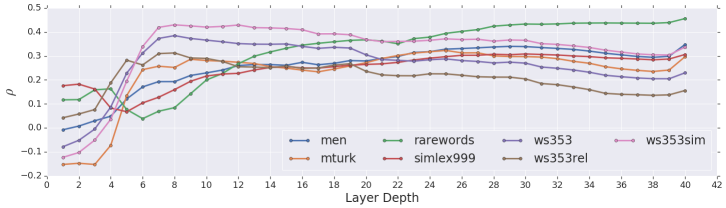
Figure 1: Performance on word similarity tasks described in Shazeer et al. (2016): Spearman’s $\rho$ measuring correlation between human annotation and cosine similarities on word representations generated from activations on different transformer layers.

In this section, we test our model’s ability to produce meaningful word-level representations. We investigate this by feeding the model single words, and evaluating its intermediate activations on word similarity tasks.

Since our model is trained to predict each individual character, activations within a word only have partial information about that word. To get a word representation, we append an empty space character at the end of the input word. The activation at the space position from the transformer’s feed-forward layer takes all characters into account, given the causal attention. To predict what follows the space, the model must have a good understanding of the preceding word, so this activation can be used as a proxy for a word representation.

To evaluate our extracted word representations, we use the word similarity tasks described in Swivel Shazeer et al. (2016). Following their evaluation methodology, we score word pairs using cosine similarity, and then measure the correlation with human ratings using Spearman’s $\rho$.

We do not expect these results to be competitive, given that our model is never trained to represent words. Moreover, the Swivel model is trained on a combination of Wikipedia and the Gigaword5 corpus Parker et al. (2011) which is composed of 3.3 billion lowercased words with discarded punctuation. They discard out-of-vocabulary words for evaluation, while we use all word pairs in the benchmark. Nevertheless, this evaluation is valuable for comparing the relative quality of representation across different layers.

Figure 1 shows Spearman’s $\rho$ across different layers of the model. We observe two main phases of performance. In the first phrase (layers 1-10), all task metrics improve with depth. In the second phase (layers 11-40), performance either plateaus or degrades slightly with depth. We suspect that the earlier layers learn general-purpose features which are linguistically relevant, while the final layers fine-tune specifically to the task of next character prediction. Interestingly, the Rare Word and SimLex999 datasets do not follow this paradigm. Their performance drops between layers 4-6, but picks up again and improves with depth (layers 6-40). We hypothesize that the model may be storing words at different depths according to their frequency. It would be interesting to investigate to what degree the improved performance of deeper LMs is due to better modeling of rare words/phrases.

Table 3 shows the best performance of our model across all layers compared to the state-of-the-art model on word similarity. The gap here is a reminder that work remains to be done on improving methods for extracting word representations from character models.

Dataset	Ours	Swivel
men Bruni et al. (2012)	0.35	0.76
mturk Radinsky et al. (2011)	0.32	0.72
rarewords Luong et al. (2013)	0.46	0.48
simlex999 Hill et al. (2014)	0.31	0.40
ws353 Finkelstein et al. (2002)	0.38	-
ws353rel Zesch et al. (2008)	0.31	0.62
ws353sim Agirre et al. (2009)	0.43	0.75

Table 3: Spearman’s $\rho$ for different datasets using our model activations. We report the best value achieved across all layers versus Swivel Shazeer et al. (2016).

6 Conclusion

We show that a tokenizer-free language model with sufficient capacity can achieve results that are competitive with word-based LMs. Our model reads raw byte-level input without the use of any text preprocessing. As such, the model has no direct access to word boundary information. Finally, we show that our model’s intermediate representations capture word-level semantic similarity and relatedness across layers.

References

- Agirre et al. (2009) Eneko Agirre, Enrique Alfonseca, Keith Hall, Jana Kravalova, Marius Paşca, and Aitor Soroa. 2009. A study on similarity and relatedness using distributional and wordnet-based approaches. In Proceedings of Human Language Technologies: The 2009 Annual Conference of the North American Chapter of the Association for Computational Linguistics, NAACL ’09, pages 19–27, Stroudsburg, PA, USA. Association for Computational Linguistics.
- Al-Rfou et al. (2019) Rami Al-Rfou, Dokook Choe, Noah Constant, Mandy Guo, and Llion Jones. 2019. Character-level language modeling with deeper self-attention. In Thirty-Third AAAI Conference on Artificial Intelligence.
- Baevski and Auli (2018) Alexei Baevski and Michael Auli. 2018. Adaptive input representations for neural language modeling. arXiv preprint arXiv:1809.10853.
- Bojanowski et al. (2017) Piotr Bojanowski, Edouard Grave, Armand Joulin, and Tomas Mikolov. 2017. Enriching word vectors with subword information. Transactions of the Association for Computational Linguistics, 5:135–146.
- Bruni et al. (2012) Elia Bruni, Gemma Boleda, Marco Baroni, and Nam-Khanh Tran. 2012. Distributional semantics in technicolor. In Proceedings of the 50th Annual Meeting of the Association for Computational Linguistics: Long Papers - Volume 1, ACL ’12, pages 136–145, Stroudsburg, PA, USA. Association for Computational Linguistics.
- Chelba et al. (2013) Ciprian Chelba, Tomas Mikolov, Mike Schuster, Qi Ge, Thorsten Brants, Phillipp Koehn, and Tony Robinson. 2013. One billion word benchmark for measuring progress in statistical language modeling. arXiv preprint arXiv:1312.3005.
- Dai et al. (2019) Zihang Dai, Zhilin Yang, Yiming Yang, William W Cohen, Jaime Carbonell, Quoc V Le, and Ruslan Salakhutdinov. 2019. Transformer-xl: Attentive language models beyond a fixed-length context. arXiv preprint arXiv:1901.02860.
- Devlin et al. (2018) Jacob Devlin, Ming-Wei Chang, Kenton Lee, and Kristina Toutanova. 2018. BERT: pre-training of deep bidirectional transformers for language understanding. CoRR, abs/1810.04805.
- Finkelstein et al. (2002) Lev Finkelstein, Evgeniy Gabrilovich, Yossi Matias, Ehud Rivlin, Zach Solan, Gadi Wolfman, and Eytan Ruppin. 2002. Placing search in context: The concept revisited. ACM Trans. Inf. Syst., 20(1):116–131.
- Gage (1994) Philip Gage. 1994. A new algorithm for data compression. C Users J., 12(2):23–38.
- Hill et al. (2014) Felix Hill, Roi Reichart, and Anna Korhonen. 2014. Simlex-999: Evaluating semantic models with (genuine) similarity estimation. CoRR, abs/1408.3456.
- Howard and Ruder (2018) Jeremy Howard and Sebastian Ruder. 2018. Universal language model fine-tuning for text classification. arXiv preprint arXiv:1801.06146.
- Kim et al. (2016) Yoon Kim, Yacine Jernite, David Sontag, and Alexander M. Rush. 2016. Character-aware neural language models. In Proceedings of the Thirtieth AAAI Conference on Artificial Intelligence, AAAI’16, pages 2741–2749. AAAI Press.
- Kingma and Ba (2014) Diederik P Kingma and Jimmy Ba. 2014. Adam: A method for stochastic optimization. arXiv preprint arXiv:1412.6980.
- Lee et al. (2016) Jason Lee, Kyunghyun Cho, and Thomas Hofmann. 2016. Fully character-level neural machine translation without explicit segmentation. CoRR, abs/1610.03017.
- Luong et al. (2013) Thang Luong, Richard Socher, and Christopher Manning. 2013. Better word representations with recursive neural networks for morphology. In Proceedings of the Seventeenth Conference on Computational Natural Language Learning, pages 104–113, Sofia, Bulgaria. Association for Computational Linguistics.
- Parker et al. (2011) Rovert Parker, David Graff, Junbo Kong, Ke Chen, and Kazuaki Maeda. 2011. English gigaword fifth edition. Philadelphia. Linguistic Data Consortium.
- Peters et al. (2018) Matthew E Peters, Mark Neumann, Mohit Iyyer, Matt Gardner, Christopher Clark, Kenton Lee, and Luke Zettlemoyer. 2018. Deep contextualized word representations. arXiv preprint arXiv:1802.05365.
- Radford et al. (2018) Alec Radford, Karthik Narasimhan, Tim Salimans, and Ilya Sutskever. 2018. Improving language understanding by generative pre-training.
- Radford et al. (2019) Alec Radford, Jeffrey Wu, Rewon Child, David Luan, Dario Amodei, and Ilya Sutskever. 2019. Language models are unsupervised multitask learners. OpenAI Blog, 1:8.
- Radinsky et al. (2011) Kira Radinsky, Eugene Agichtein, Evgeniy Gabrilovich, and Shaul Markovitch. 2011. A word at a time: Computing word relatedness using temporal semantic analysis. In Proceedings of the 20th International Conference on World Wide Web, WWW ’11, pages 337–346, New York, NY, USA. ACM.
- Sennrich et al. (2016) Rico Sennrich, Barry Haddow, and Alexandra Birch. 2016. Neural machine translation of rare words with subword units. In Proceedings of the 54th Annual Meeting of the Association for Computational Linguistics (Volume 1: Long Papers), pages 1715–1725, Berlin, Germany. Association for Computational Linguistics.
- Shazeer et al. (2018) Noam Shazeer, Youlong Cheng, Niki Parmar, Dustin Tran, Ashish Vaswani, Penporn Koanantakool, Peter Hawkins, HyoukJoong Lee, Mingsheng Hong, Cliff Young, et al. 2018. Mesh-tensorflow: Deep learning for supercomputers. In Advances in Neural Information Processing Systems, pages 10414–10423.
- Shazeer et al. (2016) Noam Shazeer, Ryan Doherty, Colin Evans, and Chris Waterson. 2016. Swivel: Improving embeddings by noticing what’s missing. CoRR, abs/1602.02215.
- Shazeer et al. (2017) Noam Shazeer, Azalia Mirhoseini, Krzysztof Maziarz, Andy Davis, Quoc Le, Geoffrey Hinton, and Jeff Dean. 2017. Outrageously large neural networks: The sparsely-gated mixture-of-experts layer. arXiv preprint arXiv:1701.06538.
- Vaswani et al. (2017) Ashish Vaswani, Noam Shazeer, Niki Parmar, Jakob Uszkoreit, Llion Jones, Aidan N Gomez, Łukasz Kaiser, and Illia Polosukhin. 2017. Attention is all you need. In Advances in neural information processing systems, pages 5998–6008.
- Zesch et al. (2008) Torsten Zesch, Christof Müller, and Iryna Gurevych. 2008. Using wiktionary for computing semantic relatedness. In Proceedings of the 23rd National Conference on Artificial Intelligence - Volume 2, AAAI’08, pages 861–866. AAAI Press.