Carbon, oxygen, and iron abundances in disk and halo stars

The abundances of carbon, oxygen, and iron in late-type stars are important parameters in exoplanetary and stellar physics, as well as key tracers of stellar populations and Galactic chemical evolution. However, standard spectroscopic abundance analyses can be prone to severe systematic errors, based on the assumption that the stellar atmosphere is one-dimensional (1D) and hydrostatic, and by ignoring departures from local thermodynamic equilibrium (LTE). In order to address this, we carried out three-dimensional (3D) non-LTE radiative transfer calculations for C I and O I, and 3D LTE radiative transfer calculations for Fe II, across the stagger-grid of 3D hydrodynamic model atmospheres. The absolute 3D non-LTE versus 1D LTE abundance corrections can be as severe as $-0.3\,\mathrm{dex}$ for C I lines in low-metallicity F dwarfs, and $-0.6\,\mathrm{dex}$ for O I lines in high-metallicity F dwarfs. The 3D LTE versus 1D LTE abundance corrections for Fe II lines are less severe, typically less than $+0.15\,\mathrm{dex}$. We used the corrections in a re-analysis of carbon, oxygen, and iron in $187$ F and G dwarfs in the Galactic disk and halo. Applying the differential 3D non-LTE corrections to 1D LTE abundances visibly reduces the scatter in the abundance plots. The thick disk and high-$\upalpha$ halo population rise in carbon and oxygen with decreasing metallicity, and reach a maximum of $\mathrm{\left[C/Fe\right]}\approx 0.2$ and a plateau of $\mathrm{\left[O/Fe\right]}\approx 0.6$ at $\mathrm{\left[Fe/H\right]}\approx-1.0$. The low-$\upalpha$ halo population is qualitatively similar, albeit offset towards lower metallicities and with larger scatter. Nevertheless, these populations overlap in the $\mathrm{\left[C/O\right]}$ versus $\mathrm{\left[O/H\right]}$ plane, decreasing to a plateau of $\mathrm{\left[C/O\right]}\approx-0.6$ below $\mathrm{\left[O/H\right]}\approx-1.0$. In the thin-disk, stars having confirmed planet detections tend to have higher values of $\mathrm{C/O}$ at given $\mathrm{\left[O/H\right]}$; this potential signature of planet formation is only apparent after applying the abundance corrections to the 1D LTE results. Our grids of line-by-line abundance corrections are publicly available and can be readily used to improve the accuracy of spectroscopic analyses of late-type stars.

1 Introduction

Carbon, oxygen, and iron are among the most interesting elements in astrophysics. They are two of the most important sources of opacity in stellar interiors, while carbon and oxygen are also catalysts in the CNO cycle and affect energy generation. Hence, they have a large influence on stellar structure (e.g. Basu & Antia 2008) and stellar evolution (e.g. VandenBerg et al. 2012). They are also important in the context of exoplanets, providing insight into their formation properties, compositions, and atmospheres (e.g. Johnson et al., 2012; Molaverdikhani et al., 2019).

The role of carbon, oxygen, and iron as diagnostics of stellar populations and Galactic chemical evolution is of particular interest. All three elements are released into the cosmos by core-collapse supernova of massive stars ($M\gtrsim 8\,M_{\odot}$); carbon and oxygen form through hydrostatic helium burning in their cores and iron forms during the explosion itself (e.g. Woosley et al., 2002). Carbon could also be released into the cosmos by massive stars before they explode via metal-line driven, metallicity-dependent winds, especially from Wolf-Rayet (WR) stars (e.g. Limongi & Chieffi, 2018). In addition, carbon is dredged up by thermal pulses in asymptotic giant branch (AGB) stars and released into the cosmos through mass loss (e.g. Karakas & Lattanzio, 2014). Lastly, significant iron is formed at later Galactic times via the radioactive decay of ${}^{56}\mathrm{Ni}$ in Type Ia supernova (e.g. Nomoto et al., 2013). Thus, the different abundance ratios of these three elements can be used to probe different astrophysical phenomena, occurring on different timescales, and associated with stars of different masses (e.g. Chiappini et al., 2003; Carigi et al., 2005; Kobayashi et al., 2006; Cescutti et al., 2009; Berg et al., 2016, 2019).

There is already literature on the abundances of these elements in the atmospheres of late-type stars, both in the disk (e.g. Delgado Mena et al., 2010; Nakajima & Sorahana, 2016; Suárez-Andrés et al., 2017) and metal-poor halo (e.g. Akerman et al., 2004; Cayrel et al., 2004; Fabbian et al., 2009b; Yong et al., 2013; Amarsi et al., 2019b). In particular, Nissen et al. (2014) measured carbon, oxygen, and iron abundances in $152$ F and G dwarfs with $-1.8\lesssim\mathrm{\left[Fe/H\right]}\lesssim+0.5$ in both the halo and the disk. The introduction of that paper includes a review of earlier studies of late-type stars. Later studies have generally supported the various conclusions of that work, concerning for example the elemental abundance separation of the thin and thick disks, the low- and high-$\upalpha$ halo populations (see Nissen & Schuster, 2010, 2011), and their mean Galactic chemical evolutions (e.g. Hawkins et al., 2015; Hayes et al., 2018). Furthermore, different studies (e.g. Teske et al., 2014; Brewer & Fischer, 2016; Bedell et al., 2018; Suárez-Andrés et al., 2018) now generally agree that exoplanet host stars do not typically have high enough ratios of carbon to oxygen to form carbon planets (Kuchner & Seager, 2005; Moriarty et al., 2014).

The results of Nissen et al. (2014) and similar studies can be considered precise in two ways. First, the observed spectra are of high spectral resolution (resolving power $R=\lambda/\Delta\lambda\gtrsim 40000$ in this case) and have high signal-to-noise ratios ($\mathrm{S/N}\gtrsim 100$); consequently, the measured equivalent widths have relatively small random errors. Second, the sample size is large enough for statistically-significant conclusions to be drawn.

However, systematic modelling errors can limit the accuracy of spectroscopic studies. Standard spectroscopic analyses of late-type stars are based on the assumption that stellar atmospheres are one-dimensional (1D) and hydrostatic, and that the atmospheric matter satisfies Boltzmann-Saha excitation and ionisation balance as is implied by local thermodynamic equilibrium (LTE). These two assumptions can impart significant errors on the inferred stellar parameters and elemental abundances, that vary depending on the parameters of the star under investigation, and depending on the spectral line(s) under investigation (e.g. Asplund, 2005).

Nevertheless, the outlook on stellar spectroscopy is promising. It is now possible to carry out highly realistic spectroscopic analyses of late-type stars, owing to advances in three-dimensional (3D) hydrodynamic modelling of stellar atmospheres (e.g. Tremblay et al., 2013; Collet et al., 2018) and in 3D non-LTE radiative transfer post-processing of these model atmospheres (e.g. Sbordone et al., 2010; Amarsi et al., 2016a), combined with progress in atomic astrophysics (e.g. Barklem, 2016a) not least in the area of ab initio calculations for inelastic collisions with electrons (e.g. Barklem et al., 2017) and with atomic hydrogen (e.g. Barklem, 2016b; Belyaev et al., 2018). A short review about the state-of-the-art can be found in Sect. 2.4 of Nissen & Gustafsson (2018).

There has been a particularly rapid development of 3D non-LTE methods for analysing carbon and oxygen abundances. In late-type stars, carbon and oxygen abundances can be measured using atomic lines (although carbon abundances are more commonly measured using lines of CH). Improved atomic models have recently been developed for C I (Amarsi et al., 2019a) and O I (Amarsi et al., 2018a), that utilise ab initio calculations for inelastic collisions with atomic hydrogen (Barklem, 2018; Amarsi & Barklem, 2019) such data typically being the largest source of uncertainty in non-LTE modelling (e.g. Barklem et al., 2011). It was shown that 3D non-LTE synthetic spectra based on these atomic models successfully reproduces the observed solar centre-to-limb variations of various C I and O I lines. This is a sensitive test of the atomic models and especially of the reliability of the data for inelastic collisions with atomic hydrogen (e.g. Allende Prieto et al., 2004; Steffen et al., 2015).

Recent studies of iron in late-type stars have demonstrated the potentially large impact of 3D non-LTE effects on Fe I lines (Amarsi et al., 2016b; Lind et al., 2017; Nordlander et al., 2017). However, such calculations are still prohibitively expensive for large samples of stars. Fortunately, progress can be made by focusing on Fe II lines instead. The departures from LTE in this majority species are thought to be insignificant in late-type stars, at least for Fe II lines of low excitation potential ($\mathrm{\chi_{exc.}}\lesssim 8\,\mathrm{eV}$) and at metallicities $\mathrm{\left[Fe/H\right]}\gtrsim-3.0$ (Lind et al., 2012). The impact of non-LTE abundance errors in Fe II lines are even smaller when the lines are measured differentially with respect to the Sun or to a standard star (e.g. Nissen et al., 2017). Assuming that these 1D non-LTE results for Fe II are also applicable in 3D hydrodynamic model atmospheres, and that 3D hydrodynamic simulations better represent real stellar atmospheres than 1D hydrostatic ones, it follows that 3D LTE models of Fe II lines should give iron abundances that are more reliable than those based on 1D (non-)LTE models.

Our goal here is to derive carbon, oxygen, and iron abundances in Milky Way disk and halo stars, that are both of high precision, and of improved accuracy. We present detailed 3D non-LTE radiative transfer calculations for C I and O I, and 3D LTE radiative transfer calculations for Fe II, using the code balder (Sect. 2). We explain the 3D non-LTE effects across stellar parameter space, and present extensive grids of 3D non-LTE and 1D non-LTE versus 1D LTE abundance corrections for C I and O I, and 3D LTE versus 1D LTE abundance corrections for Fe II (Sect. 3). For C I and Fe II, these are the first grids of their type to be presented in the literature; for O I, this updates the grids of Amarsi et al. (2016a), benefiting from the improvements to the atomic model described above, as well as to the 3D non-LTE radiative transfer code. Based on these abundance corrections, we present a reanalysis of precise literature data (Nissen et al., 2014; Amarsi et al., 2019b), to obtain carbon, oxygen, and iron abundances in a sample of $187$ disk and halo stars (Sect. 4). Finally, we discuss how these new measurements, of high precision and improved accuracy, alter our understanding of stellar populations, Galactic chemical evolution, and the formation of planets (Sect. 5), before presenting a short summary and some closing remarks on the outlook for precise and accurate spectroscopic analyses of late-type stars (Sect. 6).

2 3D non-LTE method

2.1 Model atmospheres

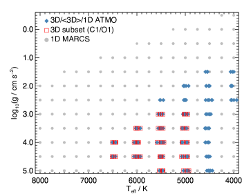
Figure 1: Kiel diagram illustrating model atmospheres in $\log{g}$—$T_{\mathrm{eff}}$ space. The $1807$ marcs nodes (grey circles) are regularly spaced in effective temperature, so model atmospheres with the same $T_{\mathrm{eff}}$ label and $\log{g}$ label but different $\mathrm{\left[Fe/H\right]}$ labels overlap in this figure. However the $164$ stagger nodes (blue diamonds) are not regularly space in effective temperature: thus, model atmospheres with different $\mathrm{\left[Fe/H\right]}$ labels are apparent as a horizontal scatter of the stagger nodes around nearby marcs nodes. The 3D LTE and 3D non-LTE calculations for C I and O I were only performed on a subset of the full stagger-grid ($74$ red squares), covering dwarfs and sub-giants.

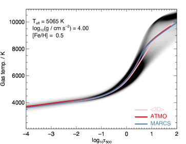
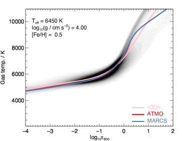
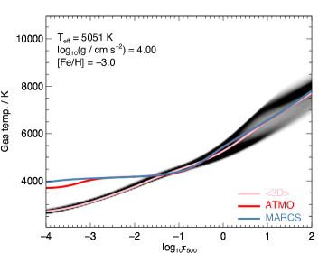
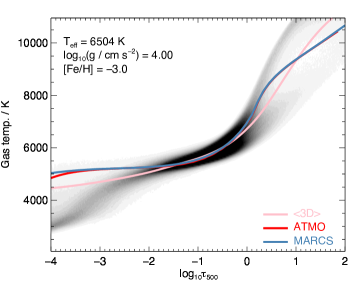
Figure 2: Gas temperature distributions in four different 3D stagger model atmospheres. The ⟨3D⟩ and 1D atmo model atmospheres are also plotted, as are the 1D marcs model atmospheres after interpolating them onto the same effective temperature. The 1D atmo and marcs model atmospheres were computed using the same fixed set of MLT parameters: $\alpha_{\text{MLT}}=1.5$, $y=0.076$, $\varv_{\text{conv}}=8.0$.

Spectrum synthesis calculations were performed on four different families of model atmospheres: 3D hydrodynamic model atmospheres from the stagger-grid (Magic et al., 2013a); 1D model atmospheres determined by averaging the 3D stagger model atmospheres (henceforth ⟨3D⟩ model atmospheres; Magic et al. 2013b); theoretical 1D hydrostatic model atmospheres from the atmo-grid (the 1D equivalent of the stagger-grid, see Appendix A of Magic et al. 2013a); and theoretical 1D hydrostatic model atmospheres from the marcs-grid (Gustafsson et al., 2008). We illustrate the grids in $\log{g}$—$T_{\mathrm{eff}}$ space in Fig. 1, and the temperature distributions for a few example models in Fig. 2.

2.1.1 3D model atmospheres

The 3D hydrodynamic model atmospheres were adopted from the stagger-grid (Magic et al., 2013a), which was constructed using the stagger-code (e.g. Nordlund & Galsgaard, 1995; Collet et al., 2018). The model atmospheres are labelled by their effective temperatures ($T_{\mathrm{eff}}$), surface gravities ($\log{g}$), and iron abundance with respect to that of the Sun ($\mathrm{\left[Fe/H\right]}$). Their chemical compositions are that of the Sun (Asplund et al., 2009), scaled by $\mathrm{\left[Fe/H\right]}$, and with $\upalpha$-element abundances enhanced by $+0.4\,\mathrm{dex}$ for $\mathrm{\left[Fe/H\right]}\leq-1.0$, to roughly account for the mean Galactic chemical evolution. The grid is not regular: the effective temperature step size varies by around $50\,\mathrm{K}$ across the grid (Fig. 1), because the emergent flux and hence the effective temperature is an output of a given simulation, rather than an input parameter.

The 3D LTE radiative transfer calculations for Fe II were performed on a set of model atmospheres of dwarfs, sub-giants, and giants. This set spans $29$ nodes in $\log{g}$—$T_{\mathrm{eff}}$ space, and up to $6$ nodes in $\mathrm{\left[Fe/H\right]}$: $4000\lesssim T_{\mathrm{eff}}/\mathrm{K}\lesssim 6500$ (in steps of roughly $500\,\mathrm{K}$), $1.5\leq\log\left(g/\mathrm{cm\,s^{-2}}\right)\leq 5.0$ (in steps of $0.5\,\mathrm{dex}$), and $-4.0\leq\mathrm{\left[Fe/H\right]}\leq 0.5$ (in steps of $1.0\,\mathrm{dex}$ for $\mathrm{\left[Fe/H\right]}\leq 0.0$). The set is illustrated in $\log{g}$—$T_{\mathrm{eff}}$ space in Fig. 1. Model atmospheres with the same $\log{g}$ labels but different $\mathrm{\left[Fe/H\right]}$ labels (input parameters in the simulations) generally have different effective temperatures. This results in a horizontal scatter in Fig. 1 about the targeted $T_{\mathrm{eff}}$ nodes that are $500\,\mathrm{K}$ apart. Although the set as described above should contain $29\times 6=174$ model atmospheres, calculations were only performed on $164$ model atmospheres; $10$ model atmospheres are missing from this grid (mainly corresponding to models having $\mathrm{\left[Fe/H\right]}=+0.5$, and having lower effective temperatures and surface gravities).

For C I and O I, the 3D non-LTE radiative calculations were performed on a subset of model atmospheres of dwarfs and sub-giants, as shown in Fig. 1. This subset spans $15$ nodes in $\log{g}$—$T_{\mathrm{eff}}$ space, and up to $5$ nodes in $\mathrm{\left[Fe/H\right]}$: $5000\lesssim T_{\mathrm{eff}}/\mathrm{K}\lesssim 6500$, $3.0\leq\log\left(g/\mathrm{cm\,s^{-2}}\right)\leq 5.0$, and $-3.0\leq\mathrm{\left[Fe/H\right]}\leq 0.5$. Calculations were performed on $74$ model atmospheres: the $T_{\mathrm{eff}}\approx 5500\,\mathrm{K}$, $\log{g}=3.0$, $\mathrm{\left[Fe/H\right]}=+0.5$ model is missing from this grid.

Prior to carrying out the 3D non-LTE calculations, the model atmospheres were re-sampled and re-grided, from their original Cartesian mesh having $240\times 240\times 230$ physical grid-points, to one having $80\times 80\times 220$ physical grid-points (Sect. 2.1.1 of Amarsi et al. 2018b). Calculations were performed on typically five snapshots of each model atmosphere, equally spaced in stellar time, from which temporally-averaged emergent line fluxes could be determined.

2.1.2 ⟨3D⟩ model atmospheres

In this work, ⟨3D⟩ model atmospheres were taken from the averaged stagger-grid presented in Magic et al. (2013b). The line formation calculations on these model atmospheres were only used to study the general behaviour of departure coefficients (Sect. 3.1); however, ⟨3D⟩ non-LTE versus 1D LTE abundance corrections were also computed, and are available upon request. The ⟨3D⟩ model atmospheres have 1D geometry, but were determined from the 3D stagger model atmospheres. Specifically, in this work the ⟨3D⟩ models are horizontal- and temporal-averages (on surfaces of constant Rosseland mean optical depth) of the gas temperature, logarithmic gas density, and logarithmic electron number density (Magic et al., 2013b). For all three elements, radiative transfer calculations were performed on the entire set of ⟨3D⟩ model atmospheres depicted in Fig. 1.

In principle, the effective temperature can change after averaging the 3D model atmosphere. These changes were not taken into account here: in other words, the $T_{\mathrm{eff}}$ label of the ⟨3D⟩ model atmosphere is identical to that of the stagger model atmosphere from which they were constructed. The illustration in Fig. 2 suggests that any changes to the effective temperature are in any case small.

2.1.3 1D model atmospheres

Theoretical 1D hydrostatic model atmospheres were adopted from the atmo-grid (Appendix A of Magic et al. 2013a). The atmo model atmospheres are the 1D versions of the stagger model atmospheres, using the same radiative transfer solver, angle quadrature, and binned opacities, and computed to have exactly the same effective temperatures, surface gravities, and chemical compositions, as their 3D equivalents. Thus, the 3D non-LTE versus 1D LTE and 3D LTE versus 1D LTE abundance corrections derived (Sect. 2.5) and presented (Sect. 3.2) here are based on stagger and atmo model atmospheres, to make them as differential as possible. For all three elements, radiative transfer calculations were performed on the entire set of atmo model atmospheres depicted in Fig. 1.

In addition, calculations were performed on $1807$ theoretical 1D hydrostatic model atmospheres adopted from the standard marcs-grid (Gustafsson et al., 2008). Compared to the stagger- and atmo-grids, the marcs-grid has the benefits of of using a monochromatic opacity-sampling treatment for the radiative transfer, and of being finer and more extended in stellar parameter space. For these reasons, 1D non-LTE versus 1D LTE abundance corrections for C I and O I based on marcs model atmospheres are also presented here.

The predicted atmospheric structure, and hence the resultant LTE and non-LTE emergent line fluxes, are in practice very similar between the atmo and marcs model atmospheres, as is evident in Fig. 2. This is in part because the two grids adopt the same implementation of the Mixing Length Theory (MLT; Böhm-Vitense, 1958; Henyey et al., 1965) to model the convective flux, using the same fixed set of MLT parameters: $\alpha_{\text{MLT}}=1.5$, $y=0.076$, $\varv_{\text{conv}}=8.0$. Both sets of theoretical 1D model atmospheres effectively enforce radiative equilibrium in the upper layers: Fig. 2 demonstrates that in the metal-poor regime, this leads them to significantly overestimating the temperature of the upper layers, where in reality the temperature is set by the competing effects of radiative heating and adiabatic cooling (e.g. Asplund et al., 1999).

As with the stagger, ⟨3D⟩, and atmo model atmospheres, the marcs model atmospheres are labelled by $T_{\mathrm{eff}}$, $\log{g}$, and $\mathrm{\left[Fe/H\right]}$; however, their chemical compositions are based on an older compilation of solar abundances (Grevesse et al., 2007), and the $\upalpha$-element abundances are enhanced by $0.1\,\mathrm{dex}$ for each step of $0.25\,\mathrm{dex}$ from $\mathrm{\left[Fe/H\right]}=0.0$ to $\mathrm{\left[Fe/H\right]}=-1.0$. For all three elements, radiative transfer calculations were performed on the entire set of marcs model atmospheres depicted in Fig. 1. This set spans $4000\leq T_{\mathrm{eff}}/\mathrm{K}\leq 8000$ (in steps of $250\,\mathrm{K}$), $-0.5\leq\log\left(g/\mathrm{cm\,s^{-2}}\right)\leq 5.0$ (in steps of $0.5\,\mathrm{dex}$), and $-5.0\leq\mathrm{\left[Fe/H\right]}\leq 0.5$ (in steps of $0.25$ to $1.0\,\mathrm{dex}$). Following Buder et al. (2018), for $\log{g}\geq 4.0$ plane-parallel model atmospheres computed with a microturbulence of $1.0\,\mathrm{km\,s^{-1}}$ were adopted; otherwise, solar-mass spherically-symmetric model atmospheres computed with a microturbulence of $2.0\,\mathrm{km\,s^{-1}}$ were adopted.

2.2 Non-LTE atomic models

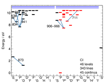
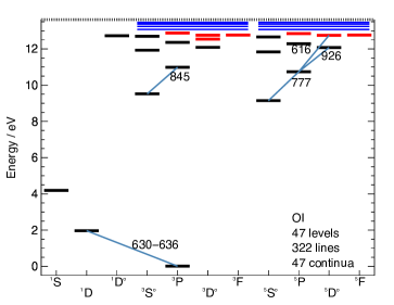
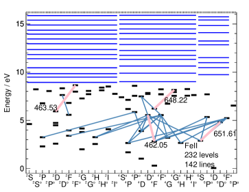
Figure 3: Grotrian term diagrams of the atomic models for C I and O I used for the non-LTE iterations. Also shown is a Grotrian term diagram for Fe II, based on which LTE emergent line fluxes were calculated. Levels for which fine structure has been collapsed are shown in red, and super levels are shown as long horizontal blue lines at the top of the figures. The transitions for which emergent line fluxes and abundance corrections were calculated are shown, connecting different energy levels. Their approximate wavelengths in air ($\mathrm{nm}$) are indicated; for Fe II this is done only for the four lines for which the 3D LTE versus 1D LTE abundance corrections are shown in Fig. 8.

For C I, the ‘No-FS’ atomic model presented in Amarsi et al. (2019a) was adopted here. This model is composed of $46$ levels of C I plus the ground state of C II, $343$ radiative bound-bound transitions, and $45$ radiative bound-free transitions in total. For O I, the ‘reduced’ atomic model presented in Amarsi et al. (2018a) was adopted here. This model is composed of $47$ levels of O I plus the three lowest levels of O II, $322$ radiative bound-bound transitions, and $47$ radiative bound-free transitions in total. We illustrate the atomic models used for the non-LTE iterations in Fig. 3; full details can be found in the above references.

A simple atomic model was also constructed for Fe II, which we illustrate this model in Fig. 3. By using this atomic model, the calculations for this species were carried out in the same way as for C I and O I, using the exact same 3D non-LTE code that we discuss in Sect. 2.3, albeit without performing any non-LTE iterations (for the reasons given in Sect. 1). Although the synthetic spectra were thus calculated under LTE conditions, completeness of the atomic model is important here to ensure that its partition function is consistent with that adopted by the internal equation of state module of the 3D non-LTE code. For this reason, super levels were included in the atomic model, as shown in Fig. 3.

2.3 Radiative transfer post-processing

The radiative transfer post-processing of the model atmospheres was carried out using balder. This is a 3D non-LTE MPI-parallelised FORTRAN code that both solves the equations of statistical equilibrium and calculates the normalised, disk-integrated emergent spectrum. It is based on multi3d (Leenaarts & Carlsson, 2009), but has various important modifications in particular concerning the parallelisation scheme and the equation of state and opacities (Amarsi et al., 2016b), the emergent spectrum solver (Amarsi et al., 2018b), and the statistical equilibrium solver (Amarsi et al., 2019a).

Emergent line fluxes for Fe II lines were calculated by balder in LTE (without any non-LTE iterations, for the reasons given in Sect. 1). For C I and O I, non-LTE iterations were carried out by balder first, using the atomic models described in Sect. 2.2. After the solutions had converged, emergent line fluxes were calculated by balder using comprehensive atomic models that include all fine structure. Emergent line fluxes were calculated only for specific lines, as we discuss in Sect. 2.4.

The calculations on the 3D, ⟨3D⟩, and 1D model atmospheres (Sect. 2.1) follow an approach that is very similar to that described in Amarsi et al. (2018b), and that paper can be consulted for further details. Here, we just note that the main difference between the calculations on the 3D model atmospheres, and on the ⟨3D⟩ and 1D model atmospheres, pertains to the broadening of disk-averaged, temporally-averaged spectral lines effected by temperature and velocity gradients as well as oscillatory motions. These effects are naturally accounted for during the post-processing of 3D hydrodynamic model atmospheres (e.g. Asplund et al., 2000). In contrast, post-processing of ⟨3D⟩ and 1D model atmospheres generally needs to include extra broadening parameters: microturbulence $\mathrm{\xi_{mic}}$ and macroturbulence $\mathrm{\xi_{mac}}$ (e.g. Chapter 17 of Gray 2008). Here, the calculations on ⟨3D⟩ and 1D model atmospheres were performed for three different values of depth-independent microturbulence: $\xi=0.0$, $1.0$, and $2.0\,\mathrm{km\,s^{-1}}$. The current study relies primarily on abundance corrections based on equivalent widths (Sect. 2.5, Sect. 3.2), rather than on spectrum fitting, and consequently macroturbulence, which by definition conserves the equivalent width, is not considered here.

The equation of state and background opacities — all line (bound-bound) and continuous (bound-free and free-free) opacities not already included in the atomic model — were computed by the blue module within balder, once given the temperature, density, and chemical composition of the model atmosphere. As in previous work (see Sect. 2.1.2 of Amarsi et al. 2016b), the background continuous opacities were computed on the fly, whereas the background line opacities were precomputed on regular grids of temperature, density, and chemical composition (labelled by $\mathrm{\left[Fe/H\right]}$), and interpolated onto the model atmosphere at runtime. The elemental abundances adopted by blue were generally set to the values that the model atmosphere was computed with. For the Fe II calculations, the iron abundance was always fixed to that of the model atmosphere. However for the C I and O I calculations, the carbon and oxygen abundances were respectively varied between $-0.4\leq\mathrm{\left[X/Fe\right]}\leq 1.2$, in steps of $0.4\,\mathrm{dex}$ for the 3D calculations, and in steps of $0.2\,\mathrm{dex}$ for the ⟨3D⟩ and 1D calculations, independent of the atmospheric chemical composition (labelled by $\mathrm{\left[Fe/H\right]}$).

In all cases, natural (radiative) broadening coefficients were estimated from the available line and level data. Pressure broadening due to elastic collisions with atomic hydrogen were generally based on the theory of Anstee, Barklem, and O’Mara (ABO; Anstee & O’Mara, 1995; Barklem & O’Mara, 1997; Barklem et al., 1998). For lines outside of these tables, the theory of Unsöld (1955) was used instead, with an enhancement factor of $2.0$ for C I and O I, and $1.5$ for Fe II.

2.4 Line selection

Emergent line fluxes (and subsequently equivalent widths and abundance corrections) were only determined for the C I, O I, and Fe II lines of most relevance to spectroscopic studies of late-type stars. This set of lines is larger than, and includes all of, the lines used in the subsequent re-analysis of literature data (Sect. 4). We illustrate the lines in Fig. 3 and provide a brief overview here; we provide a complete list of the adopted line parameters in the online Table 1.

The C I lines are listed in the first $17$ rows of Table 1 in Amarsi et al. (2019a). They are all in the optical and near infra-red, spanning wavelengths from $505\,\mathrm{nm}$ to $966\,\mathrm{nm}$. The $16$ permitted lines are all of high excitation potential, $\mathrm{\chi_{exc.}}\gtrsim 7.5\,\mathrm{eV}$, and with oscillator strengths $-1.6<\log{gf}<+0.3$; the forbidden, weak ($\log{gf}=-8.165$), low-excitation ($\mathrm{\chi_{exc.}}=1.264\,\mathrm{eV}$) [C I] $872.7\,\mathrm{nm}$ line is also included.

The set of O I lines include those studied by Amarsi et al. (2016a), namely the permitted O I $616\,\mathrm{nm}$ and $777\,\mathrm{nm}$ multiplets and the forbidden, low-excitation [O I] $630.0\,\mathrm{nm}$ and $636.4\,\mathrm{nm}$ lines. In this study this set is extended to include the permitted O I $844\,\mathrm{nm}$ and $926\,\mathrm{nm}$ multiplets. In contrast to Amarsi et al. (2016a), the abundance corrections presented here do not take into account the Ni I line that blends the [O I] $630.0\,\mathrm{nm}$ line (e.g. Allende Prieto et al., 2001).

The set of Fe II lines includes the same $142$ lines studied by Meléndez & Barbuy (2009). They are all in the optical and near infra-red, spanning wavelengths from $409\,\mathrm{nm}$ to $771\,\mathrm{nm}$, of low to intermediate excitation potentials, $2.6\lesssim\mathrm{\chi_{exc.}}\lesssim 6.2\,\mathrm{eV}$, and with oscillator strengths $-5.1<\log{gf}<-1.0$. This set of atomic data is perhaps the best currently available for Fe II lines, in the absence of more complete laboratory investigations (Den Hartog et al., 2019). Combined with 3D abundance corrections, these lines offer a promising way to obtain highly accurate iron abundances in late-type stars.

2.5 Definition of abundance corrections

The (absolute) abundance corrections presented in this work are based on equivalent widths, rather than on spectrum fitting. For a given atmospheric model (3D stagger, 1D atmo, 1D marcs), and a given radiative transfer post-processing approach (non-LTE, LTE), the equivalent widths of the lines listed in Sect. 2.4 were determined by directly integrating across the normalised emergent line fluxes.

The 3D non-LTE versus 1D LTE abundance correction for a given C I or O I line was then calculated as the difference between the absolute 3D non-LTE abundance $\log\epsilon^{\mathrm{3D,NLTE}}$ and the absolute 1D LTE abundance $\log\epsilon^{\mathrm{1D,LTE}}$, corresponding to the same, measured equivalent width: rCl Δ^3N_1L&= logϵ^3D,NLTE-logϵ^1D,LTE . These are generally five-dimensional functions: rCl Δ^3N_1L &= Δ^3N_1L(logϵ^1D,LTE, T_eff,logg,[Fe/H],ξ_mic) . Here, $T_{\mathrm{eff}}$, $\log{g}$, and $\mathrm{\left[Fe/H\right]}$ are the atmospheric parameters (Sect. 2.1), and $\mathrm{\xi_{mic}}$ is the microturbulence with which the 1D LTE line synthesis was performed (Sect. 2.3).

The 3D LTE versus 1D LTE abundance correction for a given Fe II line, $\Delta^{\text{3L}}_{\text{1L}}$, was calculated in a similar fashion. Here, the iron abundance is always consistent with the atmospheric chemical composition as labelled by $\mathrm{\left[Fe/H\right]}$ (Sect. 2.3). Consequently $\Delta^{\text{3N}}_{\text{1L}}$ is a four-dimensional function in this case.

The 1D non-LTE versus 1D LTE abundance corrections for C I and O I, $\Delta^{\text{1N}}_{\text{1L}}$, are also generally five-dimensional functions, and are defined in an analogous way to $\Delta^{\text{3N}}_{\text{1L}}$. For these abundance corrections between two sets of 1D calculations, the same microturbulence was assumed in both sets ($\mathrm{\xi^{1D,LTE}_{mic}}=\mathrm{\xi^{1D,NLTE}_{mic}}=\mathrm{\xi_{mic}}$). As discussed in Sect. 2.1, although the 3D (non-)LTE versus 1D LTE abundance corrections presented in this work are based on the 3D stagger and 1D atmo model atmospheres, the 1D non-LTE versus 1D LTE abundance corrections work are based only on 1D marcs model atmospheres.

For the Fe II lines, prior to calculating the abundance corrections, the equivalent widths were first interpolated onto a grid that is regularly spaced in effective temperature. This had to be done for Fe II, because the iron abundance was always forced to be consistent with the atmospheric chemical composition, labelled by $\mathrm{\left[Fe/H\right]}$, and because the stagger-grid nodes are irregular in effective temperature (Sect. 2.1), with nodes having the same $\log{g}$ label and $\mathrm{\left[Fe/H\right]}$ label generally having different effective temperatures. The resulting 3D LTE versus 1D LTE abundance corrections for Fe II are thus presented on a regular grid of effective temperatures. In contrast, this was not necessary for C I and O I, because the carbon and oxygen abundances were varied independently of $\mathrm{\left[Fe/H\right]}$. The resulting 3D non-LTE versus 1D LTE abundance corrections for C I and O I are thus presented on an irregular grid of effective temperatures, corresponding to the nodes shown in Fig. 1.

3 3D non-LTE effects across parameter space

3.1 Departure coefficients

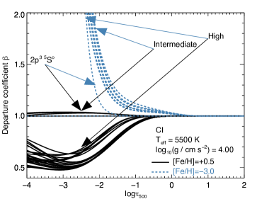
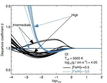
Figure 4: Departure coefficients for levels of C I (left panel), and for levels of O I (right panel), in different ⟨3D⟩ model atmospheres assuming $\mathrm{\left[C/Fe\right]}=\mathrm{\left[O/Fe\right]}=0.0$ and $\mathrm{\xi_{mic}}=1.0\,\mathrm{km\,s^{-1}}$. The levels of intermediate excitation indicated here are, for C I, $\mathrm{2p.3s\,^{3}P^{o}}$ ($7.49\,\mathrm{eV}$), $\mathrm{2p.3s\,^{1}P^{o}}$ ($7.68\,\mathrm{eV}$), and $\mathrm{2p^{3}\,{}^{3}D^{o}}$ ($7.95\,\mathrm{eV}$); and for O I, $\mathrm{2p^{3}.3s\,^{5}S^{o}}$ ($9.15\,\mathrm{eV}$) and $\mathrm{2p^{3}.3s\,^{3}S^{o}}$ ($9.52\,\mathrm{eV}$). The C I $\mathrm{2p^{3}\,{}^{5}S^{o}}$ ($4.18\,\mathrm{eV}$) is indicated separately. The levels of high excitation indicated here are the ones above these levels. In both panels, the levels of low excitation potential remain close to unity throughout the atmospheres shown.

To understand the behaviour of the abundance corrections for C I and O I lines, it is helpful to first consider how the level populations deviate from their LTE predictions in the atmospheres of different late-type stars. In Fig. 4 we plot the departure coefficients $\upbeta\equiv n_{\text{NLTE}}/n_{\text{LTE}}$ for the different C I and O I levels in the atomic models (Sect. 2.2). For clarity we only show the departure coefficients in the ⟨3D⟩ model atmospheres, which tend to follow the distributions of departure coefficients in the 3D model atmospheres (see for example Fig. 4 of Amarsi & Asplund 2017). We also only show results for the models with $T_{\mathrm{eff}}\approx 5500\,\mathrm{K}$, $\log{g}=4.00$, and two different chemical compositions corresponding to the labels $\mathrm{\left[Fe/H\right]}=+0.5$ and $-3.0$, with $\mathrm{\left[C/Fe\right]}=\mathrm{\left[O/Fe\right]}=0.0$, and $\mathrm{\xi_{mic}}=1.0\,\mathrm{km\,s^{-1}}$. The departure coefficients in stars with different effective temperatures and surface gravities show trends that are at least qualitatively similar to those discussed here.

Before discussing the behaviour of levels of intermediate and high excitation potential for C I and O I in detail, we note that for both species, the levels of low excitation potential (below around $3\,\mathrm{eV}$; see Fig. 3) have the same behaviour. Namely, their populations do not significantly deviate from their LTE predictions, across the entire grid of stellar parameters. Since C I and O I are majority species in late-type stellar atmospheres, these levels are very highly populated and are thus relatively insensitive to changes in the populations of the sparsely-populated levels of higher excitation potential. Consequently, the current model predicts negligible non-LTE effects for the [C I] $872.7\,\mathrm{nm}$ line, and for the [O I] $630.0\,\mathrm{nm}$ and $636.4\,\mathrm{nm}$ lines.

3.1.1 Levels of atomic carbon

Fig. 4 shows that, in the high metallicity case ($\mathrm{\left[Fe/H\right]}=+0.5$), the populations of the levels of intermediate excitation potential (the lower levels of the near infra-red C I lines around $906\,\mathrm{nm}$ to $966\,\mathrm{nm}$ as well as of the C I $505.2\,\mathrm{nm}$ and $538.0\,\mathrm{nm}$ lines) are close to unity (in the main line-forming regions $-1.0\lesssim\log{\tau_{500}}\lesssim 0.5$; see Fig. 1 of Amarsi et al. 2019a). The populations of the levels of high excitation potential (the upper levels of the aforementioned lines) drop slightly below unity. This behaviour is driven by photon losses in the network of intermediate- and high-excitation C I lines, causing a population cascade downwards.

This implies a slight source function effect on the intermediate- and high-excitation C I lines in the high metallicity case. A similar effect was recently discussed for the Sun (Amarsi et al., 2019a). The line source function follows $\upbeta_{\text{upper level}}/\upbeta_{\text{lower level}}$ (Rutten, 2003), and drops below the Planck function, thus the lines are strengthened with respect to LTE.

Towards lower metallicities however, photon losses in the C I lines become less significant. Fig. 4 shows that in the low metallicity case ($\mathrm{\left[Fe/H\right]}=-3.0$) the populations of the levels of intermediate and high excitation potential rise above unity in the ⟨3D⟩ model atmospheres, Non-thermal UV photons pump the various C I lines around $160$ to $250\,\mathrm{nm}$ that connect the levels of low excitation potential to the levels of intermediate excitation potential, enhancing the populations of the latter. This overpopulation is then communicated to the rest of the levels, primarily via inelastic collisions with neutral hydrogen. Consequently, the departure coefficients are largest for the levels of intermediate excitation potential, and become slightly closer to unity with increasing excitation potential. The exception to this general trend with excitation potential is the $\mathrm{2p^{3}\,{}^{5}S^{o}}$ level, as can be seen in Fig. 4: this is because, being in the quintet system, it is only weakly coupled to all of the other levels in the network, which are in the singlet and triplet systems (Fig. 3).

The overexcitation effect at low metallicities is slightly enhanced in the 3D model atmospheres where steeper temperature gradients results in a larger non-thermal UV radiation field (e.g. Asplund et al., 1999). At higher metallicities, background metal lines and continua block the UV C I lines so as to make this mechanism inefficient relative to the photon loss mechanism discussed above.

Thus, at low metallicities there is an opacity effect on the intermediate- and high-excitation C I lines. The line opacity follows $\upbeta_{\text{lower level}}$ (Rutten, 2003), and the lines are again strengthened with respect to LTE.

This picture of the non-LTE effects agrees well with that presented in Sect. 3.2 of Fabbian et al. (2006). More details of the relative importance of different radiative and collisional transitions can be found in that study.

3.1.2 Levels of atomic oxygen

At first glance the departure coefficients for O I resemble those of C I discussed in Sect. 3.1.1. However, there are differences in the details that result in non-LTE effects on the O I lines that are typically much more severe in the high metallicity case ($\mathrm{\left[Fe/H\right]}=+0.5$) and much less severe in the low metallicity case ($\mathrm{\left[Fe/H\right]}=-3.0$), compared to those on C I lines.

Fig. 4 shows that, in the high metallicity case ($\mathrm{\left[Fe/H\right]}=+0.5$), the populations of the levels of intermediate excitation potential (the lower levels of the O I $777\,\mathrm{nm}$ and $844\,\mathrm{nm}$ multiplets, namely the $\mathrm{3s\,^{5}S^{o}}$ and $\mathrm{3s\,^{3}S^{o}}$ levels) rise above unity (in the main line-forming regions $-1.0\lesssim\log{\tau_{500}}\lesssim 0.5$; see Fig. 1 of Amarsi et al. 2018a). The populations of the levels of high excitation potential typically drop slightly below unity. The exceptions seen in the plot are the $\mathrm{3p\,^{5}P}$ and $\mathrm{3p\,^{3}P}$ levels (the upper levels of the O I $777\,\mathrm{nm}$ and $844\,\mathrm{nm}$ multiplets, and the lower levels of the O I $616\,\mathrm{nm}$ and $926\,\mathrm{nm}$ multiplets): these rise above unity due to efficient collisional coupling with the levels of intermediate excitation potential. Photon losses in intermediate- and high-excitation O I lines drive a population cascade downwards, similar to C I. Unlike C I however, this population flow stops at the metastable $\mathrm{3s\,^{5}S^{o}}$ level, which is efficiently coupled to the $\mathrm{3s\,^{3}S^{o}}$ level of slightly higher excitation potential (e.g. Fabbian et al., 2009a). This also means that the strength of the O I $777\,\mathrm{nm}$ multiplet can dictate the overall statistical equilibrium (Amarsi et al., 2016a).

This implies a strong opacity effect on the O I $777\,\mathrm{nm}$ and $844\,\mathrm{nm}$ multiplets in the high metallicity case that strengthens the lines with respect to LTE. The more highly excited O I $616\,\mathrm{nm}$ and $926\,\mathrm{nm}$ multiplets (Fig. 3) suffer from both an opacity effect as well as a source function effect. The latter also strengthens the lines with respect to LTE, as the line source function drops below the Planck function.

Towards lower metallicities, as with C I (Sect. 3.1.1), photon losses in the O I lines become less significant. Fig. 4 shows that in the low metallicity case ($\mathrm{\left[Fe/H\right]}=-3.0$), and at least in the main line-forming regions, levels of intermediate excitation potential stay close to unity, while the populations of the levels of high excitation potential drop slightly below unity. This is consistent with the same picture as in the high metallicity case, namely of photon losses driving a population cascade downwards, albeit with less impact owing to the O I lines being weaker.

This implies a source function effect on the O I $777\,\mathrm{nm}$ and $844\,\mathrm{nm}$ multiplets in the low metallicity case. The source function drops below the Planck function so as to strengthen the lines with respect to LTE. On the other hand, the more highly excited O I $616\,\mathrm{nm}$ and $926\,\mathrm{nm}$ multiplets form even deeper in metal-poor stellar atmospheres, where conditions are closer to LTE. These lines thus tend to suffer only very mildly from non-LTE effects towards lower metallicities.

There are no strong O I lines in the mid-UV region that connect the levels of low excitation potential to the levels of intermediate excitation potential. Consequently there is apparently no low-metallicity overexcitation effect driven by photon pumping, in contrast to C I as discussed in Sect. 3.1.1. Photon pumping through the O I $130\,\mathrm{nm}$ line would be possible (Fabbian et al., 2009a), if not for the large H I $\mathrm{Ly\upalpha}$ opacity in the atmospheres of these stars (Amarsi et al., 2015).

3.2 Abundance corrections

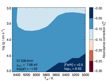
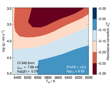
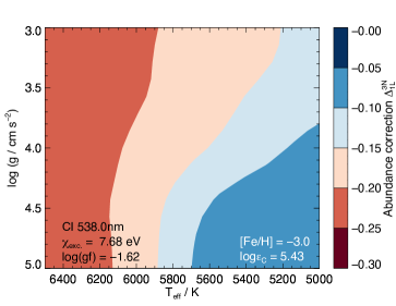
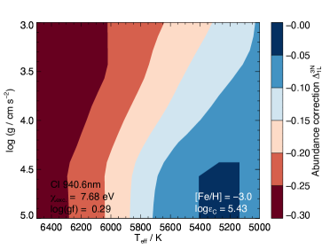
Figure 5: Kiel diagram of 3D non-LTE versus 1D LTE abundance corrections for different C I lines (columns), at different metallicities and carbon abundances (rows). The 1D microturbulence was fixed to $\mathrm{\xi_{mic}}=1.0\,\mathrm{km\,s^{-1}}$.

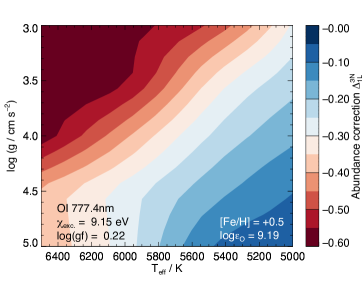
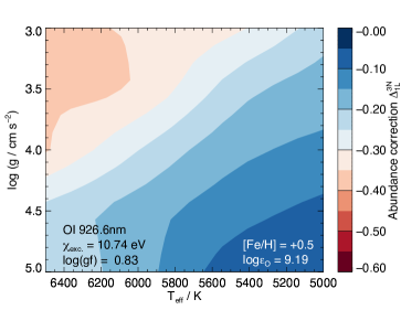
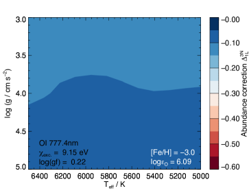
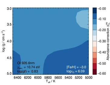
Figure 6: Kiel diagram of 3D non-LTE versus 1D LTE abundance corrections for different O I lines (columns), at different metallicities and oxygen abundances (rows). The 1D microturbulence was fixed to $\mathrm{\xi_{mic}}=1.0\,\mathrm{km\,s^{-1}}$.

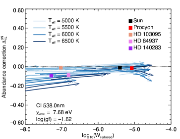
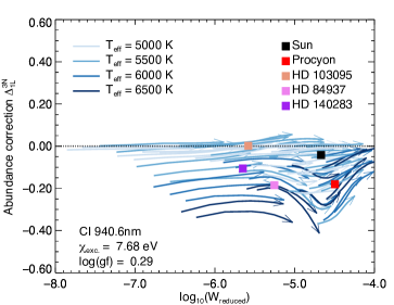
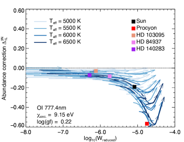
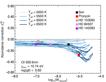
Figure 7: 3D non-LTE versus 1D LTE abundance corrections as functions of 3D non-LTE reduced equivalent widths, $W_{\text{reduced}}=W/\lambda$, for different C I and O I lines. The arrows show how the results change by increasing $\log{\epsilon_{\mathrm{C}}}$ and $\log{\epsilon_{\mathrm{O}}}$ respectively, and the curves are for fixed effective temperatures, surface gravities and metallicities, roughly corresponding to the nodes of the 3D stagger grid in Fig. 1. The 1D microturbulence was fixed to $\mathrm{\xi_{mic}}=1.0\,\mathrm{km\,s^{-1}}$. Also plotted are approximate abundance corrections for reference dwarfs, adopting the stellar parameters listed in Table 1 of Amarsi et al. (2018b) and assuming 3D non-LTE abundance ratios of $\mathrm{\left[C/Fe\right]}=\mathrm{\left[O/Fe\right]}=0.0$ for the Sun and Procyon, and of $\mathrm{\left[C/Fe\right]}=0.0$ and $\mathrm{\left[O/Fe\right]}=0.4$ for the metal-poor stars. The effective temperature of Procyon ($T_{\mathrm{eff}}\approx 6556\,\mathrm{K}$) lies slightly outside of the grid of 3D models and the abundance corrections are extrapolated here.

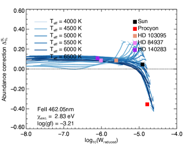
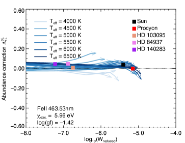
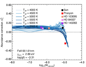
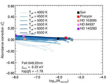
Figure 8: 3D LTE versus 1D LTE abundance corrections as functions of 3D LTE reduced equivalent widths, $W_{\text{reduced}}=W/\lambda$, for different Fe II lines. The arrows show how the results change by increasing the metallicity $\mathrm{\left[Fe/H\right]}$ (noting that the iron abundance is always kept consistent with the atmospheric chemical composition as labelled by $\mathrm{\left[Fe/H\right]}$; Sect. 2.3). Thus the curves are for fixed effective temperatures and surface gravities roughly corresponding to the nodes of the 3D stagger grid in Fig. 1. The 1D microturbulence was fixed to $\mathrm{\xi_{mic}}=1.0\,\mathrm{km\,s^{-1}}$. Also plotted are approximate abundance corrections for some reference dwarfs, adopting the stellar parameters listed in Table 1 of Amarsi et al. (2018b). The effective temperature of Procyon ($T_{\mathrm{eff}}\approx 6556\,\mathrm{K}$) lies slightly outside of the grid of 3D models and the abundance corrections are extrapolated here.

In the online Tables 2 and 3 we provide grids of 3D non-LTE versus 1D LTE abundance corrections $\Delta^{\text{3N}}_{\text{1L}}$ based on the stagger and atmo grids of model atmospheres (Fig. 1) for C I and O I lines. In the online Table 4, we provide 3D LTE versus 1D LTE abundance corrections $\Delta^{\text{3L}}_{\text{1L}}$ for Fe II lines. In addition, in the online Tables 5 and 6 we provide grids of 1D non-LTE versus 1D LTE abundance corrections $\Delta^{\text{1N}}_{\text{1L}}$ based on the more extensive marcs grid of model atmospheres (Fig. 1) for C I and O I lines. These abundance corrections can be added directly to line-by-line 1D LTE inferred abundances, to immediately improve their accuracy. Tools for interpolating these data, as well as other data (spectra, equivalent widths, and other abundance corrections) may be acquired by contacting the authors directly.

To aid intuition, in Figs 5—8 we illustrate the 3D non-LTE abundance corrections across stellar parameter space. For brevity, we only show results for representative lines, namely the C I $538.0\,\mathrm{nm}$ and $940.6\,\mathrm{nm}$ lines, the O I $777.4\,\mathrm{nm}$ and $926.6\,\mathrm{nm}$ lines, the low-excitation Fe II $462.05\,\mathrm{nm}$ and $651.61\,\mathrm{nm}$ lines, and the intermediate-excitation Fe II $463.53\,\mathrm{nm}$ and $648.22\,\mathrm{nm}$ lines. The trends in the abundance corrections with line strength and stellar parameters are at least qualitatively similar for the other lines.

It is important to note that the data and plots are of absolute abundance corrections to inferred 1D LTE values of $\log\epsilon$. In practice it is often the case that one works differentially with respect to a reference star, usually the Sun. The differential abundance correction is then usually less severe, provided that the studied star and the reference star are not too far separated in stellar parameter space.

3.2.1 Forbidden C I and O I lines

The forbidden C I and O I lines do not suffer from non-LTE effects, as discussed in Sect. 3.1. They do however suffer from 3D effects, albeit only slightly. These effects are typically of the order $0.05\,\mathrm{dex}$, as reported elsewhere: for the [O I] $630.0\,\mathrm{nm}$ and $636.4\,\mathrm{nm}$ lines see Amarsi et al. (2016a), and for the [C I] $872.7\,\mathrm{nm}$ line in the Sun see Amarsi et al. (2019a).

3.2.2 Permitted C I lines

In general, 1D LTE modelling of permitted C I lines leads to overestimated carbon abundances, across the entire parameter space under consideration here, as shown in Fig. 5. This is mainly driven by significant departures from LTE. The nature of the non-LTE effects is such that they always act to strengthen the permitted lines, as discussed in Sect. 3.1.

At high metallicities Fig. 5 shows that the 3D non-LTE versus 1D LTE abundance corrections become more severe towards higher effective temperatures and lower surface gravities. This is because at high metallicities the non-LTE effects are driven by photon losses in C I lines of intermediate and high excitation potential (Sect. 3.1), and these lines become stronger towards higher effective temperatures and lower surface gravities.

Towards lower metallicities, Fig. 5 shows that the 3D non-LTE versus 1D LTE abundance corrections become more severe, where the nature of the non-LTE effect is different: namely, the effect is one of overexcitation driven by photon pumping through C I lines in the UV (Sect. 3.1). This effect is dependent on the non-thermal UV radiation, which increases towards higher effective temperatures. Therefore at low metallicities the abundance corrections become more severe towards higher effective temperatures.

Consequently, for C I lines the most severe (absolute) 3D non-LTE versus 1D LTE abundance corrections are for metal-poor stars of high effective temperature. Fig. 5 shows that for such stars, the abundance corrections can be in excess of $-0.3\,\mathrm{dex}$ for C I lines in the near infra-red. However, the abundance corrections are somewhat less severe for the C I lines in the optical, which form deeper in the atmosphere. (see for example the contribution functions in Fig. 1 of Amarsi et al. 2019a).

In Fig. 7 the 3D non-LTE versus 1D LTE abundance corrections are plotted against (reduced) equivalent widths, for fixed stellar parameters ($T_{\mathrm{eff}}$, $\log{g}$, $\mathrm{\left[Fe/H\right]}$) but varying carbon abundance. At lower line strength, corresponding to lower metallicity, the trend of more severe abundance corrections towards increasing effective temperature, as discussed above, is immediately apparent. At higher metallicities, the abundance corrections increase with increasing line strength, and there is some indication that they turn over once the line is saturated. This signature is even clearer for O I, and we discuss it further in Sect. 3.2.3.

The absolute 3D non-LTE versus 1D LTE abundance corrections can be large at low metallicities. This means that typically, the differential abundance corrections with respect to the Sun are also quite large. For the C I $940.6\,\mathrm{nm}$ line the abundance correction is around $-0.05\,\mathrm{dex}$ for the Sun (Fig. 7), which means that if the absolute abundance correction for a given metal-poor star is $-0.3\,\mathrm{dex}$, the differential abundance correction is still as severe as $-0.25\,\mathrm{dex}$.

In light of the severity of the non-LTE effects, and in the absence of full 3D non-LTE modelling, 1D non-LTE modelling should be used for permitted C I lines. However, it should be kept in mind that when the non-LTE effects are strong they tend to be enhanced by the steeper temperature gradients present in the 3D model atmospheres. This has previously been discussed in the context of overionisation of Fe I in Amarsi et al. (2016b) and Nordlander et al. (2017), and is apparent in Amarsi et al. (2019b), where 1D non-LTE modelling still overestimates carbon abundances by around $0.05$ to $0.10\,\mathrm{dex}$ at low metallicities.

3.2.3 Permitted O I lines

In general, 1D LTE modelling of the permitted O I lines leads to overestimated oxygen abundances, across the entire parameter space under consideration here, as shown in Fig. 6. As with C I (Sect. 3.2.2), this is mainly driven by significant departures from LTE. The nature of the non-LTE effects is such that they always act to strengthen the permitted lines, as discussed in Sect. 3.1.

Fig. 6 shows that at all metallicities, the 3D non-LTE versus 1D LTE abundance corrections are more severe towards higher effective temperatures and lower surface gravities. This is because the non-LTE effects are driven by photon losses in O I lines of intermediate and high excitation potential (Sect. 3.1), and these lines become stronger towards higher effective temperatures and lower surface gravities. Unlike for C I, there is no low-metallicity overexcitation effect driven by photon pumping; thus Fig. 6 shows that the abundance corrections become less severe towards lower metallicities.

Consequently, for O I lines the most severe (absolute) 3D non-LTE versus 1D LTE abundance corrections are for metal-rich stars of high effective temperature and low surface gravity. Fig. 6 illustrates that for such stars, the abundance corrections can be in excess of $-0.6\,\mathrm{dex}$ for the O I $777\,\mathrm{nm}$ multiplet; thus, comparing with Sect. 3.2.2, the abundance corrections are more severe in O I than in C I in the worst cases. The abundance corrections are typically less severe for the O I $844\,\mathrm{nm}$, $926\,\mathrm{nm}$, and $616\,\mathrm{nm}$ multiplets, in order of decreasing severity; the latter line is highly excited and relatively weak, and forms very deep in the atmosphere where the departure coefficients are much closer to unity (Sect. 3.1).

In Fig. 7 the 3D non-LTE versus 1D LTE abundance corrections are plotted against (reduced) equivalent widths, for fixed stellar parameters ($T_{\mathrm{eff}}$, $\log{g}$, $\mathrm{\left[Fe/H\right]}$) but varying oxygen abundance. At higher metallicities, the abundance corrections increase with line strength, and turn over for reduced equivalent widths below around $-4.8\,\mathrm{dex}$. This phenomenon has previously been explained, for example in Sect. 3.1 of Lind et al. (2011) in the context of Na I lines. The abundance corrections rapidly grow when the stronger (3D) non-LTE lines enter the damping part of the curve-of-growth and develop broad wings. When this happens, efficient photon losses in the O I $777\,\mathrm{nm}$ multiplet actively drive the non-LTE effects in the system. The minimum corresponds to saturation of the O I $777\,\mathrm{nm}$ multiplet. A similar signature can be seen for the O I $926.6\,\mathrm{nm}$ line, as well as for the C I $940.6\,\mathrm{nm}$ line as pointed out in Sect. 3.2.2, however for C I it is less clear owing to a large number of C I lines influencing the statistical equilibrium.

Although the absolute 3D non-LTE versus 1D LTE abundance corrections can be very large at high metallicities, the differential abundance corrections with respect to the Sun can be more moderate. For the O I $777.4\,\mathrm{nm}$ line the abundance correction is around $-0.2\,\mathrm{dex}$ for the Sun (Fig. 7), which means that if the absolute abundance correction for a given metal-rich star is $-0.4\,\mathrm{dex}$, the differential abundance correction is only $-0.2\,\mathrm{dex}$. Similarly, if the absolute abundance correction for a given metal-poor star is close to zero, the differential abundance correction becomes $+0.2\,\mathrm{dex}$: oxygen abundances in the metal-poor regime are susceptible to 3D non-LTE effects via the solar reference abundance.

In the absence of full 3D non-LTE modelling, 1D non-LTE modelling should be used for permitted O I lines. As discussed for C I (Sect. 3.2.2), when the non-LTE effects are strong, they tend to be enhanced by the 3D effects. For the O I $777\,\mathrm{nm}$ multiplet, in the metal-rich regime, 1D non-LTE modelling can systematically overestimate oxygen abundances by of the order $0.1\,\mathrm{dex}$ (Amarsi et al., 2016a).

3.2.4 Fe II lines

By assumption, the Fe II lines do not suffer from significant non-LTE effects (see Sect. 1). Fig. 8 illustrates that the 3D LTE versus 1D LTE abundance corrections are positive for Fe II lines, at least while the lines are unsaturated (see Sect. 3.2.3). This means that 1D LTE modelling of Fe II lines results in underestimated iron abundances. The 3D effects are caused by both differences in the mean atmospheric structure, the presence of atmospheric inhomogeneities, and stellar granulation (Amarsi et al., 2016b).

The (absolute) 3D LTE versus 1D LTE abundance corrections for Fe II lines, at least while they are unsaturated, are typically in the range $-0.05$ to $+0.10\,\mathrm{dex}$ for lines of intermediate excitation potential, and $0.00$ to $+0.15\,\mathrm{dex}$ for lines of low excitation potential. They are evidently more severe for lines of low excitation potential that form higher up in the atmosphere and are sensitive to differences in the mean temperature stratification and the atmospheric inhomogeneities present in the upper layers. In contrast the lines of intermediate excitation potential form deeper and are biased towards the hot temperature upflows associated with stellar granulation.

In the absence of spectrum synthesis based on 3D model atmospheres, spectrum synthesis based on ⟨3D⟩ model atmospheres should be preferred over 1D model atmospheres, when modelling low-excitation Fe II lines, as well as when modelling lines that form higher up in the atmosphere in general (including the low-excitation forbidden C I and O I lines): the 3D LTE versus ⟨3D⟩ LTE abundance corrections are closer to zero for such lines. For lines of higher excitation potentials ($\mathrm{\chi_{exc.}}\gtrsim 4\,\mathrm{eV}$), in the absence of spectrum synthesis based on 3D model atmospheres, spectrum synthesis based on 1D model atmospheres may be more appropriate. This can be understood by considering Fig. 2: in the deep atmosphere the 1D model atmospheres have a steeper temperature gradient than the ⟨3D⟩ model atmospheres, and thus the 1D models more closely follow the hot upflows in the 3D model atmosphere.

The 3D LTE versus 1D LTE abundance corrections can become more severe towards larger line strengths as the line core becomes saturated. This can be seen for the Fe II $462.05\,\mathrm{nm}$ and $651.61\,\mathrm{nm}$ lines of low excitation potential, in Fig. 8. It is possible that this reflects the failure of the LTE assumption, and that, at the highest metallicities, strong Fe II lines of low excitation potential are susceptible to photon losses. For these reasons, at the highest metallicities it is better to avoid using strong Fe II lines of low excitation potential in spectroscopic analyses.

The absolute 3D LTE versus 1D LTE abundance corrections discussed above are slightly more severe than the differential abundance corrections relative to the Sun. The latter are typically only around $\pm 0.05\,\mathrm{dex}$. This can be seen by comparing the location of the Sun with other reference stars in Fig. 8.

4 Re-analysis of literature data

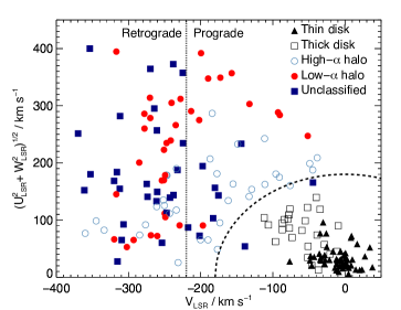
Figure 9: Toomre diagram for the entire stellar sample, corrected for the peculiar solar motion using Coşkunoǧlu et al. (2011). The kinematic information are primarily from Gaia DR2 (Gaia Collaboration et al., 2018), but for some stars where these data were missing the kinematic information come from other sources (Perryman et al., 1997; Nissen & Schuster, 2010; Anderson & Francis, 2012; Carollo et al., 2014; Kunder et al., 2017). The unclassified stars are from the VLT/UVES sample. The vertical dashed line delineates prograde and retrograde orbits, while the curved dashed line indicates a total velocity of $180\,\mathrm{km\,s^{-1}}$.

4.1 Stellar sample

The sample consists of three different data sets of F and G dwarfs: the $67$ disk stars (mainly of the thin disk, and including the Sun) in the HARPS-FEROS sample of Nissen et al. (2014); the $85$ thick-disk and halo stars in the UVES-FIES sample of Nissen et al. (2014); and the $40$ halo stars in the VLT/UVES sample of Nissen et al. (2007) which were recently re-analysed by Amarsi et al. (2019b), including the carbon-poor blue straggler G 66-30. There are five stars in common between the VLT/UVES and the UVES-FIES samples: in the subsequent analysis, the results of these common stars are presented as an error-weighted average. Consequently, the sample consists of $187$ unique stars in total, including the Sun. Full details about the observations, in particular concerning the spectral resolutions and signal-to-noise ratios of the different data, can be found in the references above.

For the HARPS-FEROS and UVES-FIES samples, stars were assigned to the same stellar populations as in Nissen et al. (2014). To summarise that work, stars were identified as belonging to the disk or halo based on whether their total velocities with respect to the local standard of rest (LSR) were less than or greater than $180\,\mathrm{km\,s^{-1}}$ (the usual discriminant between the disk and halo populations; e.g. Buder et al. 2019). The disk stars were categorised as thin- or thick-disk stars based on the 1D LTE $\upalpha$-abundance plot in Fig. 1 of Adibekyan et al. (2013), while the 1D LTE abundances of magnesium, silicon, calcium, and titanium were measured and used to separate the halo stars into low- and high-$\upalpha$ halo populations (Nissen & Schuster, 2010).

We do not attempt to assign the VLT/UVES sample stars to specific stellar populations, with the exception of the five stars in common with the UVES-FIES sample. Nevertheless, Fig. 9 shows that the majority of stars in this sample (labelled as unclassified) have a similar distribution in the Toomre diagram as those in the low-$\upalpha$ halo population, namely with a tendency towards slightly retrograde orbits and a large range in $\sqrt{\mathrm{U_{\mathrm{LSR}}^{2}+W_{\mathrm{LSR}}^{2}}}$. The majority of these stars may thus belong to the low-metallicity tail of the low-$\upalpha$ halo population; future work combining this kinematic information with information from elemental abundance ratios (see for example Figs 3, 4, and 5 of Hayes et al. 2018), will be needed to confirm this.

4.2 Stellar parameters

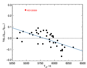
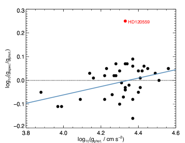
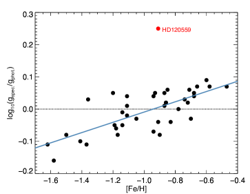
Figure 10: Differences between the spectroscopic surface gravities adopted here, and photometric surface gravities for $39$ stars in the UVES-FIES sample for which the photometry are not significantly affected by interstellar absorption and for which precise parallaxes are available from Gaia DR2. A line of best fit is overdrawn, that excludes the obvious outlier HD 120559 ($\log{g}_{\text{phot.}}=4.33$), for which the measured Gaia DR2 parallax, $\uppi=29.19\pm 0.18\,\mathrm{mas}$ may be in error; the Hipparcos parallax, $\uppi=39.42\pm 0.97\,\mathrm{mas}$, gives $\log{g}_{\text{phot.}}=4.64$, in much better agreement with the spectroscopic value ($\log{g}_{\text{spec}}=4.58$).

The effective temperatures and surface gravities adopted here are from Nissen et al. (2014) for the HARPS-FEROS and UVES-FIES samples, and those derived and used in Amarsi et al. (2019b) for the VLT/UVES sample. For the adopted 1D LTE abundances (Sect. 4.4), microturbulence is also relevant. For the HARPS-FEROS and UVES-FIES samples, these were also taken from Nissen et al. (2014), while for the VLT/UVES sample these were originally presented in Nissen et al. (2007). Errors in the choice of 1D LTE microturbulence do not severely affect the 3D non-LTE analysis presented here, because these are largely corrected for after applying the 3D non-LTE versus 1D LTE abundance corrections (which are functions of $\mathrm{\xi_{mic}}$; Sect. 2.5). We present an overview of these stellar parameters here; full details about their derivation can be found in the references above. In all of the above papers, the stellar parameters, including the chemical composition, were iterated until consistency was achieved.

For the HARPS-FEROS sample, effective temperatures were derived by Nissen et al. (2014) using $(b-y)$ and $(V-K)$ colours, and the calibration of Casagrande et al. (2010) based on the infra-red flux method. Given effective temperatures, surface gravities were derived from the fundamental relation, with absolute magnitudes derived via Hipparcos parallaxes (van Leeuwen, 2007), bolometric corrections from Casagrande et al. (2010), and stellar masses inferred via Yonsei-Yale evolutionary tracks (Yi et al., 2003). Microturbulences were inferred from a 1D LTE analysis of Fe II lines in the standard way, namely on the condition that the inferred iron abundance should not depend on line strength. For the Sun, the standard values were adopted here: $T_{\mathrm{eff}}=5772\,\mathrm{K}$ and $\log{g}=4.438$ (Prša et al., 2016), and $\mathrm{\xi_{mic}}=1.0\,\mathrm{km\,s^{-1}}$ (e.g. Holweger & Müller, 1974).

For the UVES-FIES sample, the effective temperatures and surface gravities were determined by Nissen et al. (2014) through differential 1D LTE spectroscopic analyses of weak Fe I and Fe II lines, with respect to the two standard stars HD 22879 and HD 76932. The effective temperatures and surface gravities of the standard stars were determined as per the HARPS-FEROS sample above, namely using photometry and Hipparcos parallaxes. Microturbulences were here inferred from a 1D LTE analysis of Fe I and Fe II lines.

Lastly, for the VLT/UVES sample, the effective temperatures were determined via 3D non-LTE fitting of the $\mathrm{H\upbeta}$ line in echelle spectra, as described in Amarsi et al. (2019b). The surface gravities were mainly derived using the fundamental relation as per the HARPS-FEROS sample above, except using the more precise Gaia DR2 parallaxes (Gaia Collaboration et al., 2018) instead of Hipparcos ones. The C I, O I, and Fe II lines are usually sufficiently weak in these metal-poor stars that the inferred abundances are not sensitive to the choice of microturbulence. Therefore $\mathrm{\xi_{mic}}=1.5\,\mathrm{km\,s^{-1}}$ was assumed for most of the stars in this sample.

4.3 Implications of new Gaia DR2 parallaxes

Newly available precise parallaxes from Gaia DR2 (Gaia Collaboration et al., 2018) could impact the stellar parameters derived for the HARPS-FEROS and UVES-FIES samples (the VLT/UVES sample having already being re-analysed using Gaia DR2 parallaxes as discussed in Amarsi et al. 2019b). For the HARPS-FEROS sample, the Hipparcos parallax errors are sufficiently small (corresponding to surface gravity errors of around $0.05\,\mathrm{dex}$, as discussed in Nissen et al. 2014), that there would not be a significant impact on the results if the Gaia DR2 parallaxes were used instead.

For the UVES-FIES sample, Fig. 10 illustrates slight systematic trends in the differences between the spectroscopic surface gravities adopted here and photometric surface gravities based on Gaia DR2 parallaxes, with effective temperature, surface gravity, and metallicity. The errors are at most $0.1\,\mathrm{dex}$, and largest at higher effective temperatures and lower metallicities. These trends were not apparent in Fig. 7 of Nissen et al. (2014), partly because of the larger uncertainty in the corresponding Hipparcos parallaxes adopted there, and partly because of the smaller number of stars (24) in that work with precise Hipparcos parallaxes compared to the number of stars (39) here with precise Gaia DR2 parallaxes.

The systematic trends in Fig. 10 likely arise from 3D non-LTE effects in the Fe I lines that were used to infer the spectroscopic surface gravities in Nissen et al. (2014). This was verified for the star CD -33 3337 ($T_{\mathrm{eff}}\approx 6100\,\mathrm{K}$, $\log{g}\approx 3.9$, $\mathrm{\left[Fe/H\right]}\approx-1.4$), for which the spectroscopic surface gravity is $0.11\,\mathrm{dex}$ lower than the photometric surface gravity. The 1D non-LTE versus 1D LTE abundance corrections from Lind et al. (2012) amount to around $+0.06\,\mathrm{dex}$ for representative Fe I lines, while the abundance corrections for the standard star HD 22879 amount to around $+0.03\,\mathrm{dex}$. Noting that the differential 3D non-LTE effects on Fe II lines are small between these two stars ($0.003\,\mathrm{dex}$), the differential increase in iron abundance from the Fe I lines of $+0.03\,\mathrm{dex}$ acts to increase the measured spectroscopic surface gravity of CD -33 3337 by around $0.08\,\mathrm{dex}$, and thus brings it into closer agreement with the photometric surface gravity. The residual $0.03\,\mathrm{dex}$ difference could well be due to 3D effects enhancing the non-LTE effects, as discussed in Amarsi et al. (2016b).

It is not possible to obtain precise photometric surface gravities for the entire UVES-FIES sample owing to interstellar absorption. Nevertheless, errors of $0.1\,\mathrm{dex}$ in the surface gravity have only a small impact on $\mathrm{\left[Fe/H\right]}$ (around $0.04\,\mathrm{dex}$), and a negligible impact on $\mathrm{\left[C/Fe\right]}$, $\mathrm{\left[O/Fe\right]}$, and $\mathrm{\left[C/O\right]}$ (see Table 7 of Nissen et al. 2014), and thus do not affect the main conclusions of this study.

4.4 Carbon, oxygen, and iron abundances

Iron abundances were determined from Fe II lines. For the HARPS-FEROS sample, these were the $12$ lines listed in Table 1 of Nissen et al. (2014). For the UVES-FIES and VLT/UVES samples, up to around $16$ different optical lines were adopted, for which equivalent widths have previously been presented in the literature (Nissen et al., 2002, 2004, 2007; Nissen & Schuster, 2011).

For the HARPS-FEROS and UVES-FIES samples, carbon abundances were inferred from the C I $505.2\,\mathrm{nm}$ and $538.0\,\mathrm{nm}$ lines. These lines become very weak towards lower metallicities, and for the VLT/UVES sample, the near infra-red C I lines were used instead. These lines are listed in the main text of Amarsi et al. (2019b).

For the entire sample, oxygen abundances were based on the O I $777.2\,\mathrm{nm}$, $777.4\,\mathrm{nm}$, and $777.5\,\mathrm{nm}$ lines. While Nissen et al. (2014) also measured and used the [O I] $630.0\,\mathrm{nm}$ line, we choose not to use it here, for two reasons. First, at high metallicity the [O I] $630.0\,\mathrm{nm}$ line is severely blended by a Ni I line (e.g. Allende Prieto et al., 2001) which constitutes more than $30\%$ of the equivalent width in the solar spectrum, and an even higher percentage towards higher metallicities and effective temperatures. Second, at low metallicity the [O I] $630.0\,\mathrm{nm}$ line is weak (the equivalent width in this sample is typically less than $0.5\,\mathrm{pm}$), and thus difficult to measure reliably. Thus we do not consider the [O I] $630.0\,\mathrm{nm}$ line a reliable oxygen abundance indicator for this sample.

Given the stellar parameters (Sect. 2.5), the final elemental abundances were determined by applying the 3D non-LTE versus 1D LTE abundance corrections to absolute, line-by-line 1D LTE abundances of carbon and oxygen, and the 3D LTE versus 1D LTE abundance corrections to absolute, line-by-line 1D LTE abundances of iron. Where possible, this was repeated for the Sun (included in the HARPS-FEROS sample), to derive line-by-line differential abundances that were then averaged over the different lines to obtain final estimates for $\mathrm{\left[C/H\right]}$, $\mathrm{\left[O/H\right]}$, and $\mathrm{\left[Fe/H\right]}$. For carbon and iron and for some stars, line-by-line absolute abundances had to be derived and averaged instead, owing to the lines being too blended or saturated to measure reliably in the solar spectrum. For the HARPS-FEROS and UVES-FIES samples, the 1D LTE abundances were taken from Nissen et al. (2014); for the VLT/UVES sample, they were re-derived here using our preferred stellar parameters, and our line formation calculations across the fine and extensive marcs grid.

The uncertainties in the abundances were calculated from the line-by-line variations in the inferred abundances. For stars and elements for which only a single line could be detected, the uncertainty was estimated as $\sqrt{2}$ times the largest uncertainty determined for that element in that population of stars. Finally, symmetrical uncertainties were taken from Amarsi et al. (2019b) for $\mathrm{\left[O/H\right]}$ in CD -24 17504 ($0.20\,\mathrm{dex}$) and for $\mathrm{\left[C/H\right]}$ in G 64-12 ($0.065\,\mathrm{dex}$).

We present the stellar parameters and 3D non-LTE elemental abundances in the online Table 7. For completeness, we also present the 1D non-LTE, 3D LTE, and 1D LTE results, in this online table. We plot 3D non-LTE and 1D LTE abundance ratios in Figs 11—14, and discuss the results in Sect. 5 below.

5 Discussion

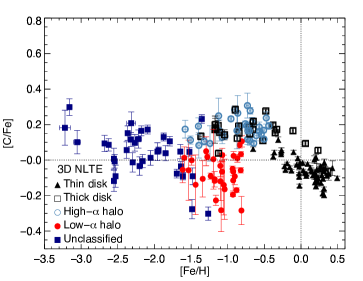
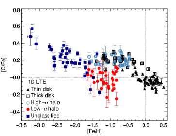
Figure 11: Carbon to iron abundance ratios for the entire stellar sample. The unclassified stars are from the VLT/UVES sample. The panels show results based on different line formation models, the 3D non-LTE model being preferred.

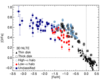
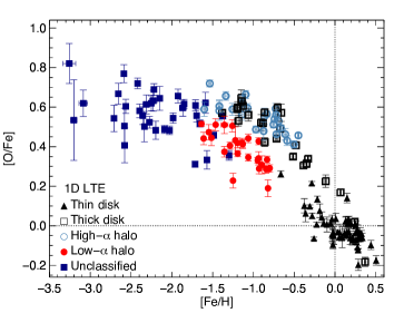
Figure 12: Oxygen to iron abundance ratios for the entire stellar sample. The unclassified stars are from the VLT/UVES sample. The panels show results based on different line formation models, the 3D non-LTE model being preferred.

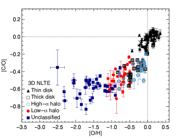
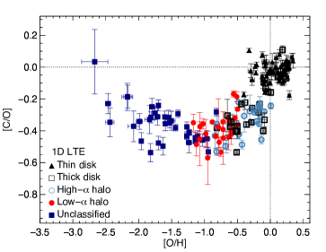
Figure 13: Carbon to oxygen abundance ratios for the entire stellar sample. The unclassified stars are from the VLT/UVES sample. The panels show results based on different line formation models, the 3D non-LTE model being preferred.

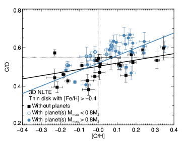
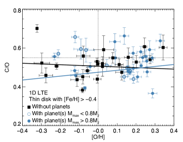
Figure 14: Carbon to oxygen abundance ratios, for thin-disk stars without and with confirmed planet detections. The latter are further separated according to the maximum planet mass in the system. The panels show results based on different line formation models, the 3D non-LTE model being preferred. The nominal solar value $\mathrm{C/O}=0.55$ is shown as a horizontal dashed line. Also plotted are error-weighted lines of best fit for stars without and with confirmed planet detections (irrespective of maximum planet mass). The error bars do not account for the systematic uncertainty in the solar carbon and oxygen abundances.

5.1 $\mathrm{\left[C/Fe\right]}$ and $\mathrm{\left[O/Fe\right]}$ in the disks and high-$\upalpha$ halo population

We verify the main results of Nissen et al. (2014) concerning the different stellar populations in Figs 11—13. There is a gap between the thin and thick disks of around $0.1\,\mathrm{dex}$ in $\mathrm{\left[C/Fe\right]}$ and $\mathrm{\left[O/Fe\right]}$ at $\mathrm{\left[Fe/H\right]}\approx 0.0$. The thick-disk stars and high-$\upalpha$ halo population stars overlap in the $\mathrm{\left[C/Fe\right]}$ and $\mathrm{\left[O/Fe\right]}$ versus $\mathrm{\left[Fe/H\right]}$ planes: this is consistent with the interpretation that the high-$\upalpha$ halo population is composed of ancient thick-disk stars that have been heated by past accretion events to obtain halo-like kinematics (Haywood et al., 2018).

Fig. 11 and Fig. 12 show that compared to the thin disk, the thick disk has higher $\mathrm{\left[C/Fe\right]}$ and $\mathrm{\left[O/Fe\right]}$ over the entire observed metallicity range, with the possible exception of at the highest $\mathrm{\left[Fe/H\right]}$: the two populations may meet at $\mathrm{\left[C/Fe\right]}\approx-0.10$, and $\mathrm{\left[O/Fe\right]}\approx-0.15$, when $\mathrm{\left[Fe/H\right]}\approx 0.4$, although the sample would need to be extended to confirm this. The thin and thick disks increase linearly in both $\mathrm{\left[C/Fe\right]}$ and $\mathrm{\left[O/Fe\right]}$ with decreasing $\mathrm{\left[Fe/H\right]}$, the thick disk seemingly rising more steeply than the thin disk. At lower metallicities, a plateau is reached in the thick disk (and high-$\upalpha$ halo population) of $\mathrm{\left[O/Fe\right]}\approx 0.6$ at $\mathrm{\left[Fe/H\right]}\approx-1.0$. These results can be interpreted by considering the cosmic origins of carbon, oxygen, and iron (Sect. 1). As oxygen is an $\upalpha$-element, the $\mathrm{\left[O/Fe\right]}$ plateau reflects a steady rate of oxygen and iron enrichment of the cosmos by core-collapse supernova. The gradual decrease of $\mathrm{\left[O/Fe\right]}$, and also of $\mathrm{\left[C/Fe\right]}$, towards higher $\mathrm{\left[Fe/H\right]}$ reflects the increasing iron enrichment from Type-Ia supernovae, which have delayed time distribution relative to core-collapse supernovae (e.g. Maoz et al. 2012).

There is a hint that $\mathrm{\left[C/Fe\right]}$ has a slight increase with increasing metallicity in the region $-1.5\lesssim\mathrm{\left[Fe/H\right]}\lesssim-1.0$, reaching a maximum of $\mathrm{\left[C/Fe\right]}\approx 0.2$ at $\mathrm{\left[Fe/H\right]}\approx-1.0$. This can be interpreted as early pollution of (presumably) the most massive AGB stars which have relatively short lifetimes ($10^{7}$ to $10^{8}$ years). This causes an increase in $\mathrm{\left[C/Fe\right]}$ with $\mathrm{\left[Fe/H\right]}$, until the contribution of iron from Type-Ia supernova becomes more dominant. These results are in agreement with measurements of $\mathrm{\left[Ba/Fe\right]}$ in Galactic halo stars, which show evidence of pollution of barium (and of other neutron-capture elements) by AGB stars, already at these low $\mathrm{\left[Fe/H\right]}\approx-1.5$ (François et al., 2007; Hansen et al., 2012).

The observed linear decrease in $\mathrm{\left[C/Fe\right]}$ (Fig. 11) and $\mathrm{\left[O/Fe\right]}$ (Fig. 12) with increasing metallicity above $\mathrm{\left[Fe/H\right]}\gtrsim 0.0$ is in contrast to some recent results. For example Hayes et al. (2018) find instead a gently rising trend of $\mathrm{\left[C/Fe\right]}$ with increasing $\mathrm{\left[Fe/H\right]}$ at super-solar metallicities, and a plateau in $\mathrm{\left[O/Fe\right]}$. The data of Hayes et al. (2018) is drawn from APOGEE DR13, where the stars are all red giants, and where the abundances of carbon and oxygen were mainly inferred from a 1D LTE analysis of infra-red CH, CO, and OH lines. In contrast, the present stellar sample is composed of F and G dwarfs, where the abundances of carbon in the high-metallicity stars were obtained from the C I $505.2\,\mathrm{nm}$ and $538.0\,\mathrm{nm}$ lines, and the abundances of oxygen were obtained from the O I $777\,\mathrm{nm}$ multiplet. Concerning the $\mathrm{\left[O/Fe\right]}$ trend, our results agree well with earlier 1D non-LTE studies of the O I $777\,\mathrm{nm}$ multiplet in dwarfs (e.g. Ramírez et al., 2013; Bensby et al., 2014; Buder et al., 2018). We speculate that this discrepancy could be alleviated if the APOGEE abundances were corrected for the severe 3D effects that are expected for molecular lines in red giants (e.g. Collet et al., 2007; Hayek et al., 2011).

5.2 $\mathrm{\left[C/O\right]}$ in the disks and high-$\upalpha$ halo population

The thin disk is systematically higher than the thick disk in the $\mathrm{\left[C/O\right]}$ versus $\mathrm{\left[O/H\right]}$ plane. Fig. 13 shows that this amounts to $\approx 0.15\,\mathrm{dex}$ in $\mathrm{\left[C/O\right]}$ at $\mathrm{\left[O/H\right]}\approx 0.0$. Furthermore, there is a clear underdensity of stars in the $\mathrm{\left[C/O\right]}$—$\mathrm{\left[O/H\right]}$ plane, in the region $\mathrm{\left[C/O\right]}\approx-0.2$ and $\mathrm{\left[O/H\right]}\approx-0.2$.

This separation of the thin disk from the thick disk (together with the high-$\upalpha$ halo population, which could be interpreted as the heated thick disk — Sect. 5.1) appears to be consistent with the Milky Way having had two main infall episodes, the latter responsible for forming the thin disk (Chiappini et al., 1997, 2001). The location of this underdensity corresponds to the discontinuity in several of the two-infall Galactic chemical evolution models recently presented in Romano et al. (2019), that marks the onset of the second infall episode (see their Fig. 1) and thus separates the younger thin disk from the older thick disk (e.g. Silva Aguirre et al. 2018).

In both the thin disk and the thick disk (and high-$\upalpha$ halo population), there are trends of increasing $\mathrm{\left[C/O\right]}$ with increasing $\mathrm{\left[O/H\right]}$. This could reflect an increasing rate of carbon enrichment from AGB stars at later epochs, or an increasing rate of carbon enrichment from metallicity-dependent winds from massive stars at later epochs, the two phenomena having degenerate elemental abundance signatures (see Sect. 1).

5.3 The low-metallicity stars

The low- and high-$\upalpha$ halo populations clearly separate into low and high groups in both the $\mathrm{\left[C/Fe\right]}$ and $\mathrm{\left[O/Fe\right]}$ versus $\mathrm{\left[Fe/H\right]}$ planes in Figs 11—12. The high-$\upalpha$ halo population can perhaps be interpreted as the heated thick disk, and we thus discuss the results for those stars in the previous subsections, Sects 5.1—5.2.

If the unclassified stars from the VLT/UVES sample are in fact primarily belonging to the low-$\upalpha$ halo population (Sect. 4.1), then it appears that the trends of $\mathrm{\left[C/Fe\right]}$ and $\mathrm{\left[O/Fe\right]}$ versus $\mathrm{\left[Fe/H\right]}$ for this combined set of low-metallicity stars are qualitatively similar to that of the high-$\upalpha$ halo population, albeit with a larger scatter, and offset towards lower metallicities. Namely, $\mathrm{\left[C/Fe\right]}$ has a mild rise with decreasing $\mathrm{\left[Fe/H\right]}$, while $\mathrm{\left[O/Fe\right]}$ has a steeper rise with decreasing $\mathrm{\left[Fe/H\right]}$ (see Sect. 5.1).

The trends inferred here for oxygen in the low-$\upalpha$ halo population are similar to those found in dwarf satellite galaxies via red giant stars (e.g. Hill et al., 2019). The same is true for carbon (e.g. Kirby et al., 2015; Skúladóttir et al., 2015; Lardo et al., 2016), after taking into account mixing in the red giant branch stars which results in an offset in $\mathrm{\left[C/Fe\right]}$ (e.g. Gratton et al., 2000; Spite et al., 2006). One interpretation of these findings, combined with information from other elemental abundance ratios, as well as kinematics and ages (Nissen & Schuster, 2010, 2011, 2012; Schuster et al., 2012), is that the low-$\upalpha$ halo is a younger population, composed of stars accreted in a past merger event with a dwarf satellite galaxy (Gaia Enceladus; Helmi et al., 2018).

If the low-$\upalpha$ halo population is to be interpreted as an accreted dwarf galaxy, one would expect that the knee in the $\mathrm{\left[\upalpha/Fe\right]}$ versus $\mathrm{\left[Fe/H\right]}$ plane is shifted to lower metallicities, reflecting the weaker star formation rate in less-massive systems (e.g. Tolstoy et al., 2009). Recent Galactic chemical evolution modelling suggest that this knee could be at around $\mathrm{\left[Fe/H\right]}\approx-2.5$ (Vincenzo et al., 2019). The corresponding plateau value of $\mathrm{\left[O/Fe\right]}\approx 0.7$ at the lowest metallicities $\mathrm{\left[Fe/H\right]}\lesssim-2.5$ in the unclassified stars, is roughly $0.1\,\mathrm{dex}$ higher than that of the high-$\upalpha$ halo population. This is consistent with the metallicity dependence of theoretical core-collapse supernovae yields, which predict $\mathrm{\left[O/Fe\right]}$ to be $\approx 0.15$ dex higher at $\mathrm{\left[Fe/H\right]}\approx-3$ compared to at solar metallicity (Kobayashi et al., 2006). Similarly, theoretical predictions indicate that $\mathrm{\left[C/Fe\right]}$ in the yields of core-collapse supernovae might increase towards lower metallicities (Kobayashi et al., 2006; Heger & Woosley, 2010).

Interestingly, in the $\mathrm{\left[C/O\right]}$ versus $\mathrm{\left[O/H\right]}$ plane (Fig. 13), there is not clear evidence for an offset between the low-$\upalpha$ halo population and the thick disk/high-$\upalpha$ halo population. Rather, the low-$\upalpha$ halo population continues the trend of decreasing $\mathrm{\left[C/O\right]}$ with decreasing $\mathrm{\left[O/H\right]}$. The unclassified stars, which are possibly dominated by the low-$\upalpha$ halo population (Sect. 4.1), form a plateau of $\mathrm{\left[C/O\right]}\approx-0.6$ below $\mathrm{\left[O/H\right]}\approx-1.0$. This plateau could be interpreted as reflecting primary carbon and oxygen nucleosynthesis from the cores of massive stars at earlier epochs, with a negligible contribution from AGB stars or metallicity-dependent winds from massive stars (see Sect. 1).

The most oxygen-poor star in Fig. 13 is CD -24 17504. Given the uncertainties, it is not clear if this star is in fact an outlier to the mean trend: the large error bars reflect the difficulty in reliably measuring the equivalent width of the O I $777\,\mathrm{nm}$ multiplet (see Fig. 4 of Fabbian et al. 2009b). If the star is indeed an outlier, this may reflect its uncertain status as a so-called carbon-enhanced metal-poor (CEMP) star (having $\mathrm{\left[C/Fe\right]}>0.7$; Aoki et al. 2007). A 1D LTE analysis of CH lines in this star suggests that it does belong to this category, with $\mathrm{\left[C/Fe\right]}\approx 1.1$ (Jacobson & Frebel, 2015). However our 3D non-LTE analysis of C I lines implies $\mathrm{\left[C/Fe\right]}\approx 0.3$: strictly speaking not a CEMP star, however still with a moderate enhancement of carbon. More discussion of this star, and two other stars in this sample that were previously reported as CEMP stars (G 64-12 and G 64-36; Placco et al. 2016), can be found in Amarsi et al. (2019b) and Norris & Yong (2019).

5.4 $\mathrm{C/O}$ in stars with and without confirmed planet detections

Given the importance of $\mathrm{C/O}$ on planet formation and characterisation (e.g. Brewer & Fischer, 2016), we briefly investigate the implications of our results on our understanding of exoplanets. In Fig. 14 we illustrate $\mathrm{C/O}$ versus $\mathrm{\left[O/H\right]}$ for thin-disk stars with and without confirmed planet detections, drawing on data from the NASA exoplanet archive (Akeson et al., 2013). By plotting $\mathrm{C/O}$ versus $\mathrm{\left[O/H\right]}$, rather than histograms of $\mathrm{C/O}$ or even $\mathrm{C/O}$ versus $\mathrm{\left[Fe/H\right]}$, it is easier to disentangle the effects of Galactic chemical evolution; while restricting the analysis to a single population (here thin-disk stars) partially removes systematics arising from age differences.

The 3D non-LTE results shown in Fig. 14 indicate that, at least for $\mathrm{\left[O/H\right]}\gtrsim 0.0$, thin-disk stars with confirmed planet detections have larger values of $\mathrm{C/O}$ than stars without confirmed planet detections at given $\mathrm{\left[O/H\right]}$. A similar result was found by Pavlenko et al. (2019), however the signature is much stronger here. There is no apparent bias with planetary mass, apart from that stars with higher metallicities (here traced by $\mathrm{\left[O/H\right]}$) tend to host more massive planets (e.g. Fischer & Valenti, 2005; Johnson et al., 2010; Adibekyan, 2019). The mean rising trend in the plot is a result of the increasing production of carbon at later cosmic times (Sect. 5.2).

The result that $\mathrm{C/O}$ is higher in stars with confirmed planet detections than in stars without confirmed planet detections, could possibly be extrapolated to say that protoplanetary disks with higher values of $\mathrm{C/O}$ give rise to more planets, or at least to more planets that are massive. The high binding energy of the $\mathrm{CO}$ molecule makes the value of $\mathrm{C/O}$ a sensitive parameter of the protoplanetary disk chemistry, and it is possible that $\mathrm{C/O}$ could play some intrinsic role in the formation efficiency of planets.

5.5 Implications of 3D non-LTE spectral line formation

It is clear from comparing the 3D non-LTE and 1D LTE results in in Figs 11—14 that using improved line formation models reduces the scatter about the mean trends in the elemental abundances. The reduction in scatter is most apparent in the $\mathrm{\left[C/O\right]}$ and $\mathrm{C/O}$ versus $\mathrm{\left[O/H\right]}$ diagrams. In particular, the 3D non-LTE results suggest that thin-disk stars with confirmed planet detections have larger values of $\mathrm{C/O}$ than stars without confirmed planet detections at given $\mathrm{\left[O/H\right]}$ (Sect. 5.4), while this signature is not apparent in the analogous 1D LTE results (Fig. 14).

Using 3D non-LTE line formation models not only impacts the scatter in the abundance ratios, but also the mean trends. For carbon, although the 1D LTE $\mathrm{\left[C/Fe\right]}$ versus $\mathrm{\left[Fe/H\right]}$ trend in Fig. 11 rises steeply towards lower metallicities, the $\mathrm{\left[C/Fe\right]}$ versus $\mathrm{\left[Fe/H\right]}$ trend is much flatter. This is because for C I, the (absolute and differential) 3D non-LTE versus 1D LTE abundance corrections are negative and are more severe towards lower metallicities (reaching $-0.3\,\mathrm{dex}$ for the near infra-red C I lines; Sect. 3.2.2).

It is important to note that other carbon abundance diagnostics are also susceptible to large systematic errors: in particular, negative and severe 3D LTE versus 1D LTE abundance corrections are expected for CH lines (reaching as much as $-1.0\,\mathrm{dex}$; e.g. Collet et al., 2006; Gallagher et al., 2016, 2017). Thus 1D LTE analyses significantly overestimate carbon abundances in metal-poor stars and thus the fraction of CEMP stars in our Galaxy (Amarsi et al., 2019b; Norris & Yong, 2019).

For oxygen, the 3D non-LTE $\mathrm{\left[O/Fe\right]}$ versus $\mathrm{\left[Fe/H\right]}$ trend in Fig. 12 is steeper in both the metal-rich regime, and in the metal-poor regime, than the corresponding 1D LTE trend. This is because for O I there are severe negative absolute 3D non-LTE versus 1D LTE abundance corrections at high metallicities (reaching $-0.6\,\mathrm{dex}$ for the O I $777\,\mathrm{nm}$ multiplet; Sect. 3.2.3). This corresponds to moderate negative differential abundance corrections with respect to the Sun (the solar absolute abundance corrections are around $-0.2\,\mathrm{dex}$ for the O I $777\,\mathrm{nm}$ multiplet.) At low metallicities however, the absolute abundance corrections for O I lines are closer to zero, and consequently the differential abundance corrections with respect to the Sun are significant, and positive (Sect. 3.2.3).

The 3D non-LTE $\mathrm{\left[C/O\right]}$ versus $\mathrm{\left[O/H\right]}$ trend in Fig. 13 is strikingly different to the analogous 1D LTE trend, as a result of the differential 3D non-LTE abundance corrections going in opposite directions for C I and O I in the low metallicity regime. While the 3D non-LTE trend is monotonic, the 1D LTE trend turns over at $\mathrm{\left[Fe/H\right]}\approx-1.0$, which has been interpreted as a possible nucleosynthesis signature of Population III stars (Akerman et al., 2004; Fabbian et al., 2009b) or rapidly-rotating massive Population II stars (Chiappini et al., 2006). This means that there is no longer a need to introduce exotic nucleosynthesis channels to explain the observations of carbon and oxygen abundances in metal-poor stars, as discussed in Amarsi et al. (2019b), at least down to $\mathrm{\left[O/H\right]}\approx-2.5$.

As explained in Sect. 3.2, in the absence of 3D non-LTE models, 1D non-LTE models should be used instead, at least for the high-excitation C I and O I lines discussed here. A comparison of 1D LTE, 3D LTE, 1D non-LTE, and 3D non-LTE results for the metal-poor stars can be found in (Amarsi et al., 2019b), where it is clear that the 1D non-LTE results better resemble the 3D non-LTE ones, at least compared to 1D LTE, or 3D LTE.

6 Conclusion

We have presented extensive grids of 3D non-LTE versus 1D LTE abundance corrections for C I and O I lines for FGK-type dwarfs and sub-giants with $5000\lesssim T_{\mathrm{eff}}/\mathrm{K}\lesssim 6500$, $3.0\leq\log\left(g/\mathrm{cm\,s^{-2}}\right)\leq 5.0$, and $-3.0\leq\mathrm{\left[Fe/H\right]}\leq 0.5$. We have also presented grids of 1D non-LTE versus 1D LTE abundance corrections for C I and O I lines that extend to even hotter and cooler late-type stars. The (absolute) 3D non-LTE versus 1D LTE abundance corrections can be as severe as $-0.3\,\mathrm{dex}$ for C I lines, and $-0.6\,\mathrm{dex}$ for O I lines.

In addition, we have presented 3D LTE versus 1D LTE abundance corrections for Fe II lines (which are expected to suffer negligible non-LTE effects) for late-type FGK-type dwarfs, sub-giants and giants with $4000\lesssim T_{\mathrm{eff}}/\mathrm{K}\lesssim 6500$, $1.5\leq\log\left(g/\mathrm{cm\,s^{-2}}\right)\leq 5.0$ and $-4.0\leq\mathrm{\left[Fe/H\right]}\leq 0.5$. The 3D LTE versus 1D LTE abundance corrections for Fe II lines are usually only of the order $-0.05$ to $+0.15\,\mathrm{dex}$.

We used the abundance corrections to re-analyse the carbon, oxygen, and iron abundances in $187$ F and G dwarfs previously presented in the literature. It is clear that (differential) 3D non-LTE effects significantly reduce the scatter in the results and change the mean Galactic chemical evolution trends. This is most apparent in the $\mathrm{\left[C/O\right]}$ versus $\mathrm{\left[O/H\right]}$ plane, where severe 3D non-LTE versus 1D LTE differential abundance corrections in both C I and O I work in the same direction such that, while 1D LTE models predict a sharp minimum of $\mathrm{\left[C/O\right]}\approx-0.5$ at $\mathrm{\left[O/H\right]}\approx-1.0$, 3D non-LTE models predict $\mathrm{\left[C/O\right]}$ to monotonically decrease with decreasing $\mathrm{\left[O/H\right]}$, to a plateau of $\mathrm{\left[C/O\right]}\approx-0.6$ below $\mathrm{\left[O/H\right]}\approx-1.0$. Some discussion of this result in the context of proposed exotic nucleosynthetic signatures can be found in Amarsi et al. 2019b.

The reduction in scatter due to the 3D non-LTE abundance corrections also has implications on studies of exoplanets. We found evidence that, at a given value of $\mathrm{\left[O/H\right]}$, thin-disk stars with higher values of $\mathrm{C/O}$ tend to be more likely to host planets. This result could be used to constrain planet formation models, the physics of which are still not perfectly understood.

Although beyond the scope of this work, the improved carbon and (in particular) oxygen abundances presented here have implications on stellar ages as determined from stellar evolutionary models. They have a direct influence on the rate of burning via the CNO cycle, and are important sources of opacity in stellar interiors (e.g. Salaris et al., 1993); these factors can make the shapes and locations of stellar isochrones in the Hertzsprung-Russell diagram sensitive to the assumed abundances (e.g. Bond et al., 2013). Given the significant differential abundance corrections for both C I and O I at low metallicity, this should be relevant not only in the context of absolute ages of the oldest stars (e.g. VandenBerg et al., 2014), but also in the context of differential ages of low-$\upalpha$ and high-$\upalpha$ halo population stars (Ge et al., 2016).

The grids of line-by-line abundance corrections are presented in the online Tables via the CDS. It is extremely cheap and simple to apply these abundance corrections to 1D LTE abundances, to improve the accuracy of spectroscopic analyses of late-type stars. We demonstrated this here for $187$ stars, but in principle, as long as line-by-line 1D LTE abundances are available, this approach can easily be applied to the extremely large spectroscopic surveys of over $10^{6}$ stars, which are planned or currently underway (e.g. Dalton et al., 2016; Buder et al., 2018; Jönsson et al., 2018; de Jong et al., 2019).