Physics Informed Data Driven model for Flood Prediction: Application of Deep Learning in prediction of urban flood development

Abstract

Flash floods in urban areas occur with increasing frequency. Detecting these floods would greatly help alleviate human and economic losses. However, current flood prediction methods are either too slow or too simplified to capture the flood development in details. Using Deep Neural Networks, this work aims at boosting the computational speed of a physics-based 2-D urban flood prediction method, governed by the Shallow Water Equation (SWE). Convolutional Neural Networks(CNN) and conditional Generative Adversarial Neural Networks(cGANs) are applied to extract the dynamics of flood from the data simulated by a Partial Differential Equation(PDE) solver. The performance of the data-driven model is evaluated in terms of Mean Squared Error(MSE) and Peak Signal to Noise Ratio(PSNR). The deep learning-based, data-driven flood prediction model is shown to be able to provide precise real-time predictions of flood development. Implementation codes can be found in the link.

Abstract

Floods are attacking urban area more and more frequently. A real-time flood system which can reflect the detailed flood development and provide on-time prediction of flood can help alleviate the loss caused by floods. The present flood prediction methods are either too slow or too simplified to capture the flood development in 2-D sense. This work boosts the computation speed of a physics-based flood prediction method which is governed by Shallow Water Equation(SWE) and is able to predict the flood development in 2-D sense with Deep Neural networks. Convolutional Neural Networks(CNN) and Generative Adversarial Neural Networks(GANs) are applied to learn the dynamics from the data simulated by a Partial Differential Equation(PDE) solver.

1 Introduction

Floods are the most common disaster worldwide Berz (2000). Every year, floods cause more than $6,000$ casualties, and have an estimated cost of $25$ billion dollars Berz (2000). Several flood mitigation strategies exist, including flood channels, early warning systems Krzhizhanovskaya et al. (2011), temporary flood barriers, etc. Few (2003). Among all these strategies, flood monitoring is one of the most inexpensive, and most resilient strategy to uncertainties Montz and Gruntfest (2002). Hence, timely, accurate early warning systems could lead to a dramatic reduction of flood-caused injuries and fatalities. Given the very large areas that require monitoring, mobile sensing platforms, such as Unmanned Air Vehicles (UAVs), are most suitable for such problems. UAVs have been used for a variety of monitoring applications, including air pollution monitoring in Alvear et al. (2017) and flood monitoring in Mohammed et al. (2014); Dunbabin and Marques (2012).

Accurate, real-time prediction of flash flood onset and progression is a challenging problem. It requires the fusion of measurements with computationally-intensive flood propagation models to estimate the water levels and velocities over an entire region. Modern estimation techniques are mainly based on a Bayesian Tracking procedure with two steps: Prior Update and Measurement Update. These are conducted recursively to update the estimated state of the system Bergman (1999). This process is summarized in Fig.1. The first step, prior update, depends on the prior knowledge that people have about the system and its dynamics. The update can be executed using either (1) a physics-based model describing the propagation of water flows or (2) using purely statistical methods. Statistical methods usually require historical data. Lots of researches in this field apply time-series prediction models to collected data from fixed gauge stations to predict flood or river stream flows Khac-Tien Nguyen and Hock-Chye Chua (2012); Damle and Yalcin (2007); Xiong et al. (2001); Laio et al. (2003); Valipour et al. (2012, 2013); Basha et al. (2008). Neural Networks and its variants are also frequently used to extract the stream fluctuation rules from historical data and predict future floods Coulibaly et al. (2000); Sattari et al. (2012); Elsafi (2014); Humphrey et al. (2016); Sit and Demir (2019). Interested readers can refer to Mosavi et al. (2018) for a detailed review for the application of machine learning techniques to flood predictions. However, statistical prediction methods can only give a broad prediction for river systems or flood basins. Furthermore, the lack of historical data in urban areas makes it troublesome to use statistical methods to address the issue of real-time urban flood prediction. Instead, physical models which depend on Partial Differential Equations (PDEs) can simulate, thus predict, flood development given the realistic settings.

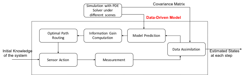
Figure 1: Overview of the estimation process for a real-time flood monitoring system. The focus of the present article is the data-driven model.

Flood dynamics are usually governed by the Shallow Water Equation (SWE) Vreugdenhil (2013). With its origin in the Navier-Stokes Equation, SWE is widely applied to environmental flow simulation. The general characteristic of shallow water flows is that the vertical dimension is much smaller than the horizontal scale. Although SWE shows a 3-D attribute due to the bottom friction Vreugdenhil (2013), in most cases, it’s sufficient to average over the vertical horizon to get the 2-D SWE. Since Alcrudo and Garcia-Navarro (1993), the finite volume method is popular for the numerical simulation of SWE. The main progresses of the numerical solutions for SWE are listed as follows. Anastasiou and Chan (1997) extended the finite volume based numerical solution of SWE to unstructured mesh. Kurganov and Levy (2002); Audusse et al. (2004); Kurganov et al. (2007); Liang and Marche (2009) contributes to the ’well-balanced’ numerical simulation of SWE which can preserve numerical stability of the dry area and still water. People also worked out the well-balanced solution of the wet-dry front problem in SWE  Horváth et al. (2015); Bollermann et al. (2013).

Recent research probes implementing SWE numerical simulation on Graphics Processing Units (GPU) Brodtkorb et al. (2012). Although PDE-based models can give detailed prediction for flood events in urban areas, the computation speed of the SWE solver is too slow to meet the real-time prediction requirements, especially for city-wide simulations. It can be even worse if the Monte-Carlo methods, such as the Ensemble Kalman Filter(EnKF) which is widely applied in large scale environmental systems, are used in estimation. Present physics-based real-time prediction methods rely heavily on simplifications. The 2-D domain is simplified to the catchments and links between them in which only 1-D Saint-Venant equations need to be solved  Yakowitz (1985); Georgakakos (1986); Moore et al. (1994); Bellos and Tsakiris (2016); Bout and Jetten (2018). The simplifications lead to imprecise predictions and cannot cover every corner of a city-wide area.

Recently, deep learning has risen as a promising way to extract highly non-linear relations from data LeCun et al. (2015). With its structured architecture and automatic training process with back propagation Rumelhart et al. (1988), researchers are using deep learning to solve PDEs Raissi (2018); Raissi et al. (2017a, b); Sirignano and Spiliopoulos (2018) or boost the speed of PDE solvers Tompson et al. (2017a, b); Thuerey et al. (2018); Wiewel et al. (2018); Xie et al. (2018); Chu and Thuerey (2017). Through processing the data simulated by PDE solvers, deep learning models can mimic the non-linearity carried by PDEs with a much faster computation speed in prediction. Thuerey et al. (2018); Wiewel et al. (2018); Xie et al. (2018); Chu and Thuerey (2017) follow this idea and apply different deep learning methods to problems related to the Navier-Stokes equation. However, these studies only focus on theoretical settings and haven’t been extended to large scale PDE systems.

The objective of this study is to investigate the application of deep learning to boost SWE solver speeds for the purpose of real-time flood prediction. Specifically, given an initial state and boundary conditions, the data-driven model will predict the future states subject to various inputs. Austin, Texas is targeted as the area receiving the flood (shown in Fig.2(a) and Fig.2(b)). The deep learning based, data-driven model will carry the physics governed by SWE equations and the parameters that imitate the features of the Austin area to make real-time predictions on floods. The precise data-driven model can replace SWE models to provide real-time and detailed prediction of flood evolution on a city-wide scale. To the best of our knowledge, this is the first real-time flood prediction model which can give detailed prediction of a two dimensional flood over a large spatial domain. This is also the first study that investigates deep learning to reconstruct the dynamics of the 2D SWE in a realistic urban setting.

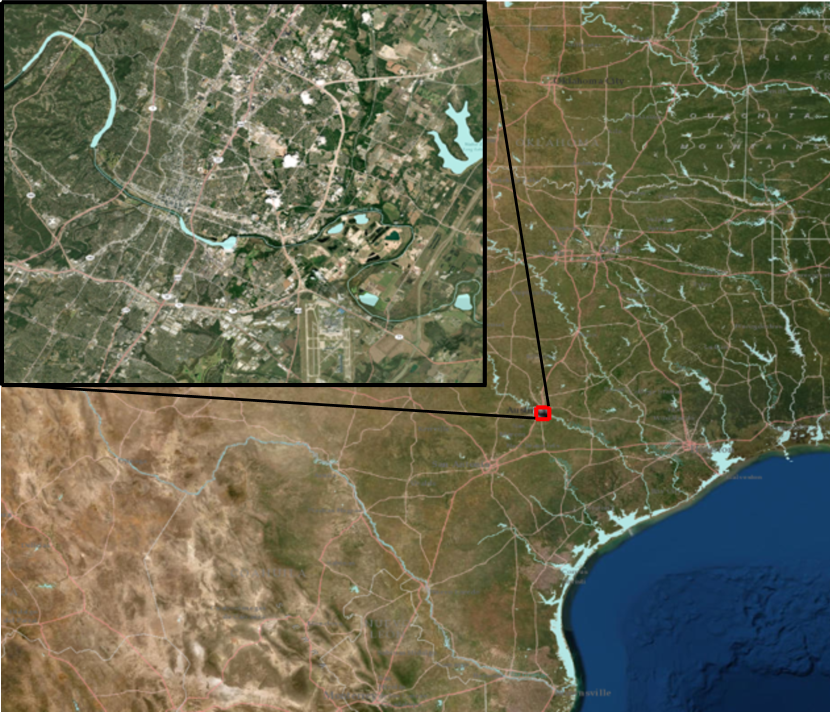
(a) The location of Austin.

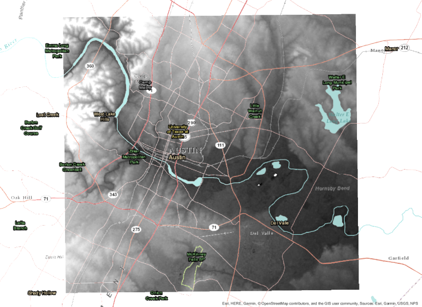
(b) The topology of Austin.

Figure 2: Map of the studied area. The left subfigure represents the subset of the state of Texas that we study in this article. The right subfigure represents an elevation map of this area.

The organization of this paper is as follows. Section 2 talks about the methodology of the study. Section 3 introduces the procedure to produce data for deep learning. The performance of deep learning based, data-driven models are evaluated and discussed in Section 4. Section 5 summarizes the study and the obtained results. Potential future works are discussed. More results and training details of the neural networks are presented in the Appendix.

2 Methodology

2.1 General Procedure

This work proposes a deep neural network that can substitute the SWE-based solver for predicting the evolution of floods. The philosophy behind this idea is simple. The deep neural network is trained on large quantities of data simulated by the SWE simulator with different initial states, inputs and boundary conditions. In numerical simulations, time steps are set to be small to achieve high precision and numerical stability while also dragging down the computation speed. The data-driven model is set to predict over a larger time step to boost the prediction speed. The general process is illustrated in Fig.3. Difficulties arise from the high dimensional inputs and outputs in learning, highly non-linear dynamics by SWE and the gaps in data scale between cases.

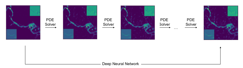
Figure 3: Overview of the objective of this work. With PDE solver, thousands of computation steps are needed to predict over a horizon of $5$ minutes. In this work, the objective is to replace the PDE solver with a deep learning model which can directly predict the states several minutes later with one step of computation to realize the real-time prediction task.

Starting from SWE, this section will go through the construction process of the data-driven model including inputs, outputs and deep learning techniques applied.

(2.1) is the incompressible shallow water equation in 2D conservative form, obtained from Tan (1992); Zoppou and Roberts (1999).

(2.1) $$\frac{\partial\mathbf{U}}{\partial t}+\bigtriangledown\mathbf{F}=\mathbf{S}$$

where $\mathbf{U}$ is the vector of conservative variables, $\mathbf{F}$ is the flux tensor and $\mathbf{S}$ is the source term. Changing Equ. (2.1) to Cartesian form will result in Equ. (2.2).

(2.2) $$\frac{\partial\mathbf{U}}{\partial t}+\frac{\partial\mathbf{E}}{\partial x}+\frac{\partial\mathbf{G}}{\partial y}=\mathbf{S}$$

where $\mathbf{E}$ and $\mathbf{G}$ are cartesian components of $\mathbf{F}$. The detailed expression of $\mathbf{U}$, $\mathbf{E}$, $\mathbf{G}$ and $\mathbf{S}$ are in (2.3).

(2.3) $$\mathbf{U}=\begin{bmatrix}h\\ uh\\ vh\end{bmatrix}\text{, }\mathbf{E}=\begin{bmatrix}uh\\ u^{2}h+gh^{2}/2\\ uvh\end{bmatrix}\text{, }\mathbf{G}=\begin{bmatrix}vh\\ uvh\\ v^{2}h+gh^{2}/2\\ \end{bmatrix}$$

Different force terms can be included in the term $\mathbf{S}$ depending on the chosen application. Here, gravity and the friction between water and ground are included as two basic terms.

(2.4) $$\mathbf{S}=\begin{bmatrix}0\\ gh(S_{g_{x}}-S_{f_{x}})\\ gh(S_{g_{y}}-S_{f_{y}})\end{bmatrix}$$

in which $S_{g}$ only depends on the gravity coefficient and the slope of the topology. With $\eta$ as friction coefficient, $S_{f}$ is defined according to Manning resistance law Gioia and Bombardelli (2001) as $S_{f_{x}}=\frac{u\eta\sqrt{u^{2}+v^{2}}}{h^{4/3}}$ and $S_{f_{y}}=\frac{v\eta\sqrt{u^{2}+v^{2}}}{h^{4/3}}$.

According to the above equations, $u$, $v$ and $h$ are the three state variables of a system governed by SWE. Let us denote $u$, $v$ and $h$ at time step $t$ as $u^{t}$, $v^{t}$ and $h^{t}$. Let us denote the $u$, $v$ and $h$ values of discrete domain as vector $\mathbf{\bar{U}}$, $\mathbf{\bar{V}}$ and $\mathbf{\bar{H}}$. Suppose $\mathbf{\phi}$ is a numerical method derived from Equ.2.2 such that

(2.5) $$\begin{bmatrix}\mathbf{\bar{U}}^{t+\delta t}\\ \mathbf{\bar{V}}^{t+\delta t}\\ \mathbf{\bar{H}}^{t+\delta t}\end{bmatrix}=\mathbf{\phi}(\begin{bmatrix}\mathbf{\bar{U}}^{t}\\ \mathbf{\bar{V}}^{t}\\ \mathbf{\bar{H}}^{t}\end{bmatrix},p^{t})$$

in which $p^{t}$ is the input to the system at time step $t$. Various numerical methods can be used to solve Equ. 2.2, though each corresponding $\phi$ will be either computationally expensive or the associated time step $\delta t$ will have to be small. As a result, the total number of computations required to solve Equ. 2.2 is huge and its execution usually takes a long time, especially in cases of large scale watersheds.

The general idea of this work is to find a deep learning model $\Phi$ that can provide precise and fast prediction of the future states of a system governed by the SWE, given the present states and forecast inputs. The function $\Phi$ is related to $\phi$ according to the following expression:

(2.6) $$\begin{split}\begin{bmatrix}\mathbf{\bar{U}}^{t+n\delta t}\\ \mathbf{\bar{V}}^{t+n\delta t}\\ \mathbf{\bar{H}}^{t+n\delta t}\end{bmatrix}&=\mathbf{\Phi}(\begin{bmatrix}\mathbf{\bar{U}}^{t}\\ \mathbf{\bar{V}}^{t}\\ \mathbf{\bar{H}}^{t}\end{bmatrix},p^{t},\dots,p^{t+(n-1)\delta t})\\ &=\mathbf{\phi}(\mathbf{\phi}(\dots\phi(\begin{bmatrix}\mathbf{\bar{U}}^{t}\\ \mathbf{\bar{V}}^{t}\\ \mathbf{\bar{H}}^{t}\end{bmatrix},p^{t}),\dots,p^{t+(n-2)\delta t}),p^{t+(n-1)\delta t})\end{split}$$

It is noticeable that only the present states $\begin{bmatrix}\mathbf{\bar{U}}^{t}\\ \mathbf{\bar{V}}^{t}\\ \mathbf{\bar{H}}^{t}\end{bmatrix}$ is included in right side of Equ. 2.5 and Equ. 2.6. As the SWE is a first order PDE and can be written in homogeneous form Zoppou and Roberts (1999), it has the Markov Property which means only present states are needed to predict future states. Thus, it is not necessary to depend on previous information. Although Recurrent Neural Network (which keeps historical information) can still be applied, Convolutional Neural Network will be enough for this task. Moreover, it was shown in Bai et al. (2018) that Convolution operations can also be applied to temporal prediction tasks.

It should be noted that only the expression of the dynamics is provided in Equ. 2.2. In order to properly pose this PDE problem, boundary condition constraints and initial conditions are needed. These constraints will be specified in Section 3.

2.2 Convolutional Neural Network

Since the data representation to the network is two-dimensional, which contains $3$ channels each pixel, Convolutional Neural Networks (CNN)s LeCun et al. (1998) are suitable for such a data representation. Convolutional layers, which apply the same parameters over each local sub-part of the images, mimic the convolution operation. This type of model greatly reduces the number of parameters needed in the neural network.

For this pixel-to-pixel regression task, a neural network architecture is applied such that the dimension of the input in each channel is first reduced while the number of channels increases. The dimension of each channel is then increased while the number of channels is reduced. The idea is illustrated in Fig. 4(b). In order to avoid vanishing gradient in deep networks, the idea of residual block extracted from ResNet He et al. (2016) is applied among the network. Residual blocks (Fig.4(a)) have been shown to ease the learning process of deep neural networks in general, owing to their ability to overcome the problem of decaying gradients. The $L_{1}$ norm loss is used in the loss function. $L_{1}$ norm loss can measure the absolute difference between predictions and targets. Comparing to $L_{1}$ norm loss, $L_{2}$ norm tends to give blurred prediction in pixel-to-pixel tasks Mirza and Osindero (2014) and thus is not employed.

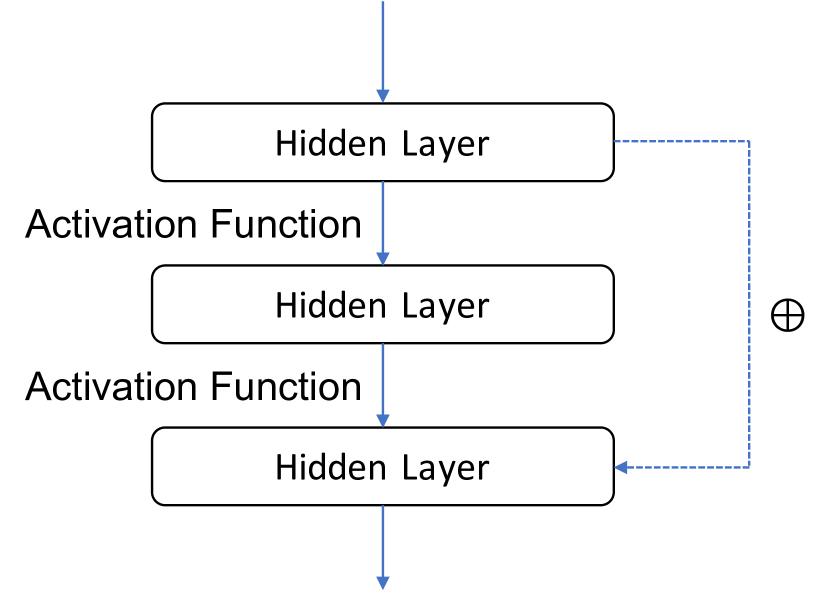
(a) Residual Block

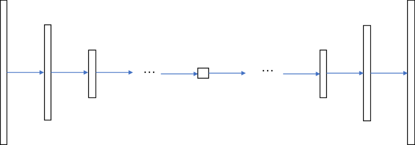
(b) Network Architecture illustration

2.3 Generative Adversarial Networks

Generative Adversarial Networks (GANs), introduced in Goodfellow et al. (2014), is a class of deep models that learn the distribution of the data. Usually, GANs consist of two deep models, a generator ${G(z;\theta_{g})}$ that attempts to generate a realistic sample from the data distribution $\sim p_{\text{data}}$ using random noise ${p_{z}(z)}$ as an input, and a discriminator ${D(x;\theta_{d})}$ that classifies these samples ${p_{g}}$ as real or fake.

(2.7) $$\min_{G}\max_{D}V(D,G)=\mathbb{E}_{{x}\sim p_{\text{data}}({x})}[\log D({x})]+\mathbb{E}_{{z}\sim p_{z}({z})}[\log(1-D(G({z})))].$$

Similarly to CNNs, Generative Adversarial networks (GANs) can also conduct pixel-to-pixel regression with conditionsl GANs. As we attempt to predict the next state of the flood based on the current state, conditional GANs Mirza and Osindero (2014) are particularly suited. In conditional GANs, we condition the input and the output with a sample from our initial states of the flood ${{f}}$. The GANs value function becomes:

(2.8) $$\min_{G}\max_{D}V(D,G)=\mathbb{E}_{{x}\sim p_{\text{data}}({x})}[\log D({x}|{f})]+\mathbb{E}_{{z}\sim p_{z}({z})}[\log(1-D(G({z}|{f})))].$$

The process of the conditional GANs is illustrated in Fig.5.

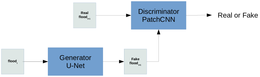
Figure 5: The GAN workflow used for flood prediction.

In fact, conditional GANs can be viewed as improving objective functions beyond CNNs, from a fixed $L1$ norm loss to a trainable neural network which can capture the structural error Dosovitskiy and Brox (2016); Li and Wand (2016); Mirza and Osindero (2014). In order to pursue both a small structural loss and absolute error between predictions and targets, $L_{1}$ norm loss and neural network based discriminator are usually mixed together in loss functions. Notice that the conditional GANs will go back to CNNs when the relative weight of $L_{1}$ norm loss is set high.

2.4 Improving the performance of conditional GANs with Kalman Filter

GANs are suitable to generating predictions following a certain type of distribution. However, this may lead to poor performance in flood prediction. At the situation of light rains (small scale inputs), the changes in flood states are so subtle that the distribution can be assumed to be static. Thus, sometimes conditional GANs cannot predict subtle changes at the beginning stage. This will cause a divergence between predictions and targets. Two ways are proposed to solve this problem. First, the weight of $L_{1}$ norm loss in loss functions can be increased to care more about subtle changes. Second, an assimilation method is raised to overcome the possible divergence of conditional GANs based models, the procedure of which is similar to the measurement update step of Kalman Filter. The details of the second method is illustrated below.

Introduced by Kalman (1960), Kalman Filter is a classical estimation technique based on two steps. The second step, referred to as the Measurement Update, can be a method of merging information from two different sources: an a-priori estimate and measurement data. Depending on the co-variance matrix, the Kalman Filter can update the system with partial observations:

(2.9) $$\mathbf{\mathbf{\hat{X}}}=\mathbf{X}+\mathbf{P}\mathbf{H}^{T}(\mathbf{H}\mathbf{P}\mathbf{H}+\mathbf{R})^{-1}(\mathbf{z}-\mathbf{H}\mathbf{X})$$

The assimilation method takes exactly the same form as Equ.2.9, though the meaning of the variables differs. Given the prediction $\mathbf{X}$ by conditional GANs and the prediction $\mathbf{z}$ by some other prediction models, $\mathbf{P}$ and $\mathbf{R}$ are the co-variance matrices of prediction error of $\mathbf{X}$ and $\mathbf{z}$ respectively. Suppose $z$ is allowed to be a partial prediction, the matrix $\mathbf{H}$ connects the prediction $\mathbf{X}$ and $\mathbf{z}$. The performance of this kind of ensemble method is shown in Fig.6. In practice, $\mathbf{z}$ can be predicted by some small neural networks which only predicts states with a small number of specific pixels. The predictions by small neural networks are expected to be more precise than conditional GANs in those pixels. With the co-variance matrix $\mathbf{P}$, surrounding areas are also updated by this step.

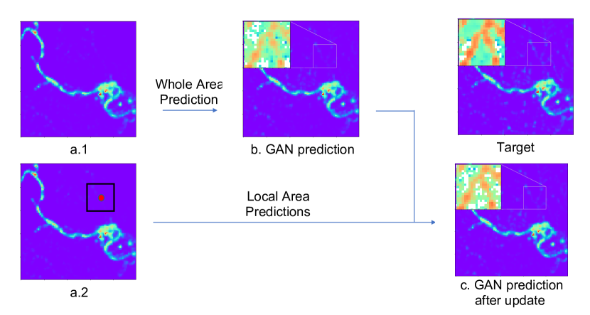
Figure 6: The demonstration of how we depend on Kalman Filter to improve the prediction performance of cGANs. a.1 and a.2 are the same input. We use a.1 and cGANs to give a whole-area prediciton(b). We use local areas(black box) in a.2 to predict the states at red dot places. Then, the prediction at red dot places are used to improve the prediction precision of the local area of b.GAN prediction. The improved result is shown in c. When predicting, we depend on around 50 spots similar to the red spot in a.2.

3 Data Preparation

In this section, the process of generating training data is detailed. To focus on learning the SWE dynamics with deep learning, the training data is generated with the following assumptions:

• The rain rate (input of the model) is set before the simulation (i.e. not forecast by this data-driven model).

• The soil properties are constant over the simulation period (hence the model is not taking into account the change of the runoff coefficient as the soil absorbs water).

• The influence of the sewers in this area is not included in the model.

It is stated in Section 2 that water depth and water momentum in the x, y directions can represent a system governed by SWE. Combining this with the above assumptions, the three states can be extended to represent flood states in urban areas.

(a) Elevation map of Austin, TX.

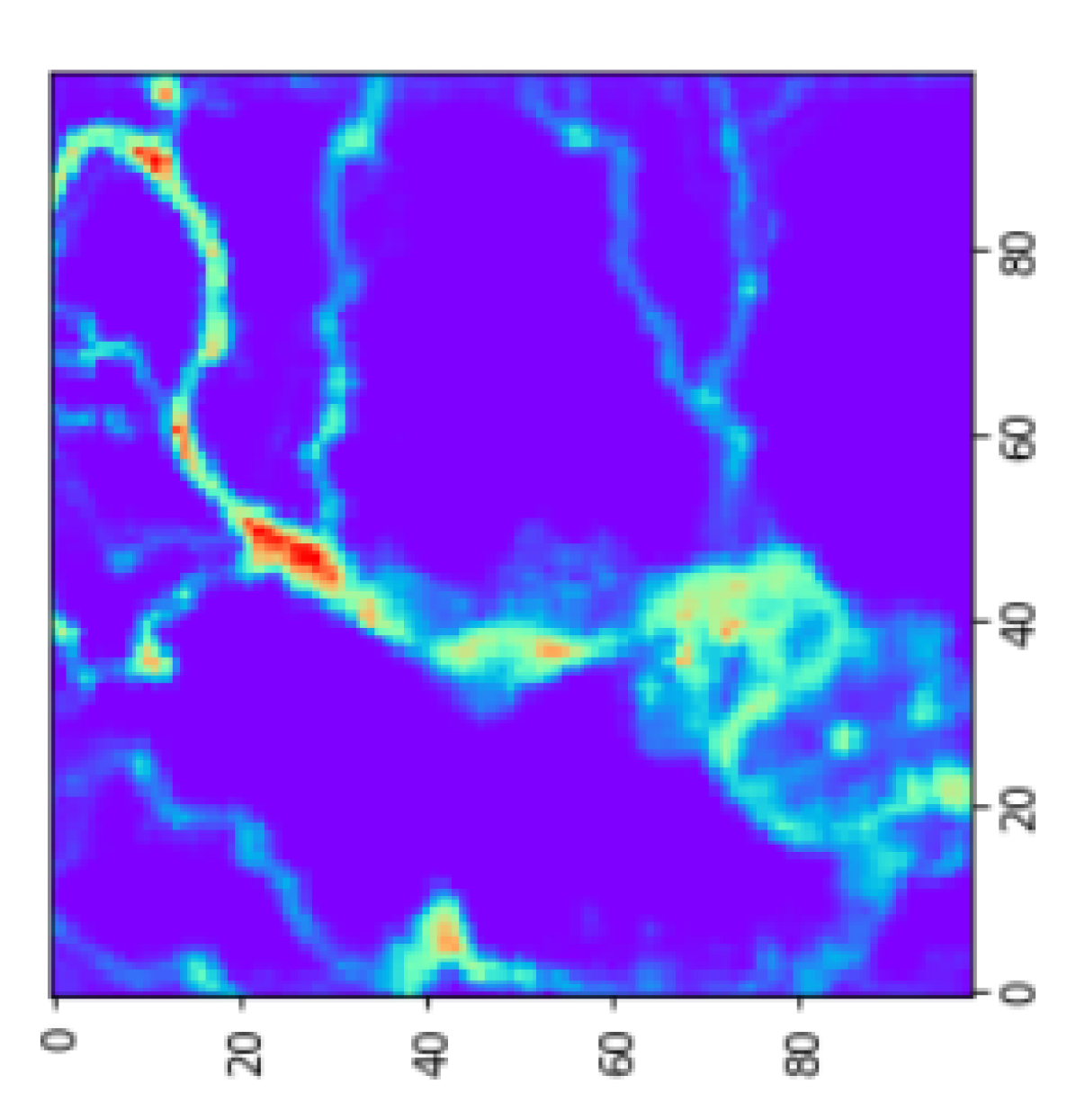
(b) Water level map associated with a simulated flood example.

Figure 7: This figure illustrates an example flood simulation. Left: illustration of the topology (the Colorado river is superimposed to the elevation map for clarity). Right: example flood simulation result using the SWE with a set rain rate function and inflows from river channels.

The numerical simulations are done in Python and consist of two steps. The first step is to compute the input map over time (rain rate), and the boundary condition functions, used to feed the PDE solver. The second step is to run the PDE solver with a set initial state, the computed boundary conditions, and the input functions. The process is shown in Fig. 8.

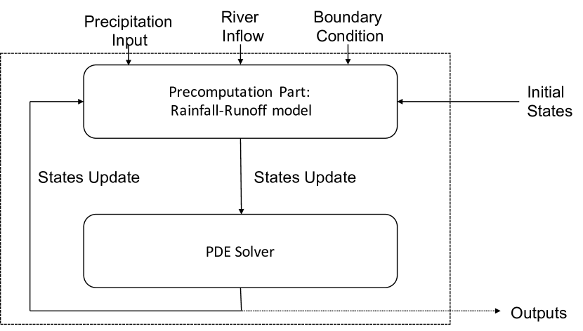
Figure 8: Computational process used for forward simulation of floods using the SWE.

The open-sourced SWE solver ANUGA Hydro developed by Roberts et al. (2015) serves as the SWE solver in the simulation. It employs a finite volume scheme to solve the 2-D SWE. Inside ANUGA, the mesh generator Triangle from Shewchuk (1996) is employed to mesh the area into Delaunay triangulations. The areas of interest (basin and creek areas) are finer meshed than other areas that are not likely to flood. Using the finite volume method, ANUGA applies the numerical scheme from Kurganov et al. (2001) to approximate the numerical flux function. The time step size of the simulation is chosen to satisfy Courant–Friedrichs–Lewy (CFL) condition Courant et al. (1928) for stability.

As mentioned in Section 1, Austin, Texas is set as the test location. The topology of this area is shown in Fig.2(b). The studied area is divided into $9$ sub-areas, and it is assumed that the precipitation density is spatially uniform within a sub-area. Besides precipitation, inflows from river channels are another input to the model. For the boundary conditions of the studied domain, static water level conditions are assumed, representing Dirichlet boundary conditions. Between each simulation, the level of boundary water depth is different and chosen randomly within a reasonable range. Although the boundary flood level is not included in the inputs of the deep learning models, it is assumed that the flood depth near the boundary area can reflect the boundary water level. Friction coefficients are chosen according to the type of soil in Austin area, using tabulated values.

A total of $1080$ different simulation configurations (combinations of different precipitation patterns, precipitation amount and inflow patterns) are simulated. In each case, the flood is simulated over an horizon of $12$ hours. For convenience, the data generated on the irregular triangle mesh is resampled onto a regular grid using interpolation. The data is thus projected on a $100\times 100$ grid, saved every $5$ minutes of simulation time.

When extracting data from the simulation results to train the neural network, a stored result is randomly taken as an input and after $30$ minutes, the simulated state serves as the output. The precipitation and inflows between these two time steps are extracted and averaged, as are the other two input channels. In total $10,000$ pairs of inputs and outputs are extracted for training, and another $2,000$ as validation data.

To summarize, each input is an image with $5$ channels of dimension $100\times 100$. The five channels corresponds to the water depth, water momentum in the $x$ direction, water momentum in the $y$ direction, the expected inflow in the next $30$ minutes, and the expected precipitation in the next $30$ minutes. The output data is a $100\times 100$ image with $3$ channels, representing the state of system $30$ minutes after the input. The training data can be found in the link .

4 Results and discussion

In order to better analyze the results of the regression, pixels in the studied domain are divided into three classes according to simulation data using K-Means MacQueen et al. (1967). The three classes respectively correspond to the Colorado River (the main river), small creeks and channels (which can flood or not), and permanently dry areas. In the Colorado river area, the water depth tends to be large and the speed of water is relatively stable. In creeks and channels, there are considerable variations in water depth and velocity during flood development. This is the area that people are most interested in. In other areas, grids are always dry, irrespective of the simulated scenario. The three classes are illustrated in Fig. 10.

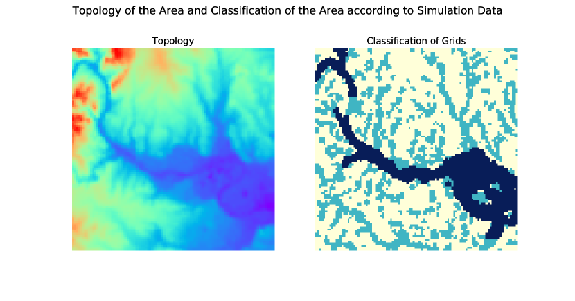
Figure 9: The Classification of the area.

Figure 10: The left subfigure represents the elevation of each grid point in our study area. The right subfigure indicates the different classes: dark grid points are the Colorado river basin, light blue areas are small channels, and white areas are dry lands.

The rest of this section serves to compare models trained under different settings. With the same CNN architecture (the optimal one), Model 1 adds noise to the inputs during the training process, while Model 2 does not. Model 3 is a conditional GANs based model, in which the discriminator only has a relatively small weight comparing to $L_{1}$ norm component in loss function. Model 3 also adds noise in the training inputs. Model 4 and Model 5 are conditional GANs based models in which the weight of the discriminator is higher than the $L_{1}$ norm component in loss function. Models 4 and 5 are identical except for the application of the assimilation step introduced in Section 2 in Model 5.

4.1 Comparison of different models

The precision and computation speed in predicting one step forward are evaluated in this subsection. The precision is measured by MSE error and the computation speed is compared based on how much the deep learning models boost the SWE solver.

Methods	Class attributes
	River	Channel	Land
Model 1	0.000376930	0.000375208	0.000026189
Model 2	0.000352408	0.000346435	0.000020496
Model 3	0.000478783	0.0005027733	0.00003498
Model 4	0.006085431	0.003261132	0.000161186
Model 5	0.004006399	0.002234181	0.000161186

Table 1: Precision of one-step prediction (water depth, x-momentum and y-momentum) with different methods in MSE sense. The results are averaged over $2000$ test cases.

Methods	Class attributes
	River	Channel	Land
Model 1	0.000313255	0.000150732	0.000013969
Model 2	0.000367964	0.000129624	0.00000875
Model 3	0.000417673	0.00022312	0.0000166921
Model 4	0.003452165	0.001244793	0.000101648
Model 5	0.002452165	0.000837835	0.000101648

Table 2: Precision of one-step precision (water depth only) with different models, in the MSE sense. The results are averaged over $2000$ test cases.

As shown in Table 1 and Table 2, CNN-based models generally have higher precision in prediction than those of GANs. Although conditional GANs has shown its advantages over figure translation tasks Mirza and Osindero (2014), it did not show many advantages over plain CNNs in the pixel-to-pixel regression task in this work. Meanwhile, it is shown that increasing the weights attached to $L_{1}$ norm in loss function can improve the performance of conditional GANs. As discussed in Section 2, discriminator in GANs can be viewed as a way to measure structural loss while $L_{1}$ norm directly measures the absolute difference between predictions and targets. Thus, it makes sense that putting more weights on $L_{1}$ norm in loss function will reduce the error measured by MSE. Model 5 also shows an improvement over Model 4, which means the assimilation approach can improve the precision of Model 4 albeit not as much as Model 3. Comparing the performance of Model 1 and Model 2, it can be seen that training without added noise will bring us a more accurate result in predicting for only one step. However, the higher precision in predicting one step ahead does not always mean a better performance in predicting the temporal evolution for a long time horizon. This will be discussed further in the next subsection.

Methods	Computation Speed
PDE Solver	$1\times$
Model 1	$50000\times$
Model 2	$50000\times$
Model 3	$50000\times$
Model 4	$50000\times$
Model 5	$10\times$

Table 3: Computational time improvements. All computations are performed on a Intel i7-7700 CPU $@$3.60GHz. Since the computational time of the PDE solver depends on the initial conditions and the inputs of the problem, the PDE solver speed is averaged over a large number of different cases.

Since the main motivation of developing a data-driven model to substitute the PDE solver is to realize the real-time prediction, the computation speed is compared in table 3 with PDE solver as baseline. To be fair, we conduct the computation of PDE solver and data-driven model on the same computer without parallel computing activated. It can be observed from the Table 3 that data-driven models boost the computation speed greatly and are fast enough to serve as prediction models for real-time flood monitoring. Furthermore, the computational speed of PDE solver is unsteady. It varies considerably with water speed and can be extremely slow when modeling fast water streams. However, the computation speed of the data-driven model is quite stable. This is a significant advantage of data-driven models for estimation tasks. Ensemble Kalman Filter(EnKF), which depends on a large number of ensembles to capture the non-linearity of the system, is usually used in estimating large scale systems. With the improvements in computation speed, the data-driven model makes it possible to apply EnKF to flood estimation tasks.

4.2 Prediction over temporal evolution

The performances of data-driven models in predicting temporal evolution are discussed in this section. In the study of numerical simulator for PDEs, stability is a main focus. Extending it to data-driven models, it is concerned whether the data-driven model can stably and realistically reproduce the dynamics carried by the SWE. For all the test cases in this subsection, data-driven models are only shown with the initial conditions and the inputs at each step. The predictions by data-driven models are compared with the predictions by SWE solver.

In order to measure the performance of each method quantitatively, MSE error and PSNR(Peak Signal to Noise Ratio) are computed for each method.

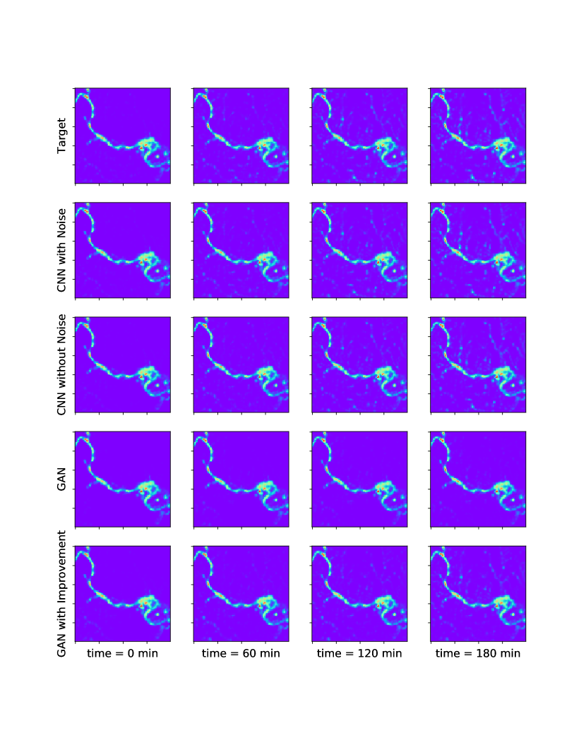
Figure 11: The comparison between targets and different deep learning based prediction methods. We compare the prediction by different methods with targets at $0$ minutes, $60$ minutes, $120$ minutes and $180$ minutes. All the methods are provided with same initial conditions and inputs. The first row is the target.

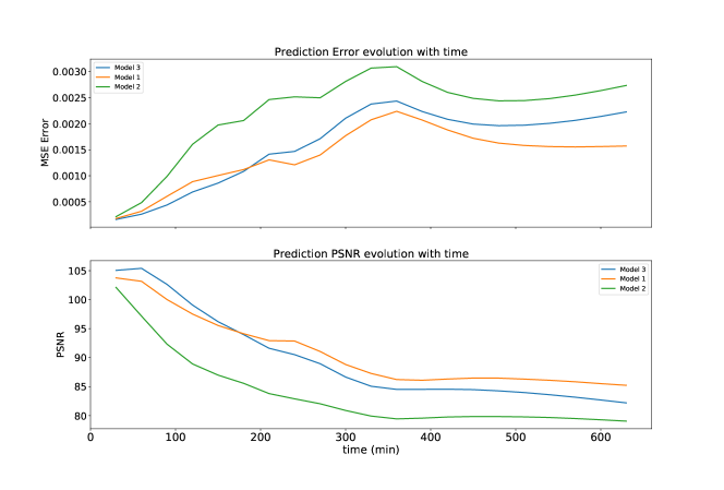
Figure 12: The comparison of performance of Model 1,2 and 3. In the first plot, the development of MSE error along time is shown. In the second plot, we present the PSNR index along time by. The results are computed under $30$ different pieces of time series data and then averaged.

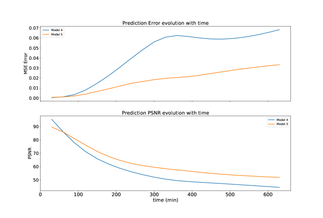
Figure 13: The comparison of performance of Model 4 and 5. In the first plot, the development of MSE error along time is shown. In the second plot, we present the PSNR index along time by. The results are computed under $30$ different pieces of time series data and then averaged.

First, let us discuss the results shown in Fig. 11. We pick a case and predict respectively with Models 1, 2, 4 and 5. The results are plotted at time=0 minutes, 60 minutes, 120 minutes and 180 minutes. We can see that the prediction results by Model 1 and Model 2 look almost the same as the target. Meanwhile, we can see that the predictions by Model 4 totally diverge from targets in creek areas. The reason behind this has been mentioned in Section 2. Trivial omits by conditional GANs accumulated in temporal evolution can lead to a noticeable divergence. With the improvements made by the posterior-adjustment step, Model 5 can also learn the development of flood, just not as effectively as Models 1 and 2. More tests can be found in the Appendix.

Let us then analyze the results quantitatively. In Fig. 12, we plot the averaged MSE and PSNR by Models 1, 2 and 3. Although it was shown in Table. 1 that Model 2 leads to higher precision than Model 1 in prediction one step, it is shown in Fig. 12 that Model 1 performs better in temporal evolution. This makes sense, as the noise added to training data mimics the imprecision of data-driven model caused by the previous prediction steps. Furthermore, although Model 3 performs worse than Model 1 and 2 in Table 1, it has a similar performance as Model 1 in temporal evolution in Fig.12. This means that lowering structural loss with a discriminator can improve the performance of a data-driven model in temporal evolution. In Fig. 13, the improvements over conditional GANs by a post-adjustment step are quantitatively illustrated along the temporal evolution.

4.3 Validation of Measurement update

It is mentioned in Section 1 that the data-driven model would be used for the real-time flood estimation purpose. It is validated in this section that the data-driven model can be applied to flood state estimation.

Model 1 is chosen as the base model. Measurement update is conducted after each prediction step. An empirical co-variance matrix is extracted from simulation data to describe the spatial correlation. In Fig. 14, it is shown that the error is greatly reduced and the PSNR is improved with the measurement update over Model 1. It means that the data-driven model can work well for flood state estimation tasks.

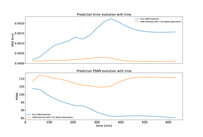
Figure 14: The comparison of performance of Model 1 and Model 1 with Measurement update from true states. In the first plot, the development of MSE error along time is shown. In the second plot, we present the PSNR index along time by. The results are computed under $30$ different pieces of time series data and then averaged.

5 Conclusion

In this work, we develop physics-informed, data-driven models to predict the evolution of a two dimensional flood in a test area of Austin, Texas. The data-driven model recovers the dynamics encoded by the 2D SWE equations and boosts the computation speed by several orders of magnitude (approximately $\times 50,000$). Compared to statistics-based and other simplified flood prediction models, the physics-informed, data-driven model provides detailed and real-time city-wide flood development predictions. This can serve as the prediction model for real-time flood monitoring, estimation, or model-predictive control applications.

Several Deep Learning techniques, including CNN and conditional GANs, are applied in constructing the learning structure and the loss functions. According to this study, appropriate CNN architectures can recover the dynamics of the 2D SWE very well. Conditional GANs can reduce the structural error of the prediction with the discriminator, though it can cause a divergence over longer time horizons. In order to overcome this divergence, an assimilation step inspired from the update step of the Kalman Filter is introduced and proves to be useful. Adding more weights to the $L_{1}$ norm term in the loss function of conditional GANs can also improve the performance. Different models are compared both qualitatively and quantitatively in Section 4. It is shown that the predictions made by a data-driven model aligns well with the results given by the SWE simulation.

Future works will involve the following aspects. First, state estimation techniques based on the physics-informed, data-driven model for flood estimation can be developed (i.e. using a classical Ensemble Kalman Filter or a Particle Filter). Second, the influence of different parameter sets with SWE on data-driven models should be studied. The parameters of the SWE, including elevation and friction coefficients, will greatly affect the outcome of the simulation. Thus, this scheme can be used to perform inverse-modeling (parameter estimation) based on actual flood data. Third, more advanced and realistic simulations can be configured to provide training data for the data-driven model. In this work, although a complex setting of an urban area with realistic topology information is studied, more detailed settings have not been specified in the model. For example, the saturation of the soil by the flood (which affects the model parameters), the sewers in urban areas, and the local impact of the dense buildings in the downtown areas have not been precisely modeled, other than by their low runoff coefficients.

References

Appendix

Training Details

CNN

Following the basic idea of Section 2, we tested several architectures and chose the highest performing. The architecture finally adopted is shown in Fig.15. The $100\times 100$ dimension is firstly scaled down and then some residual blocks are applied. The dimension is then scaled up back to $100\times 100$. The details(activation function, kernel size in each layer) can be found in Table 4. $8000$ epochs are run for each training task. We tested the performance of Stochastic Gradient Descent (SGD) and ADAM Kingma and Ba (2014). It is found that SGD and ADAM will eventually have similar testing and training errors, though ADAM has a much faster convergence rate at the beginning epochs. In terms of learning rate schedule, several popular schedules are tested, including fixed learning rate, decaying with epoch($\frac{0.001}{\sqrt{epochnum}}$) and periodic learning rate.

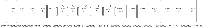
Figure 15: The general Architecture of Residual Block based Network. For the details in each layer, please refer to corresponding table in Appendix. Table4

layer 1	channel: $5\rightarrow 16$; kernel size: $5\times 5$; Stride: $1$; Padding: $0$; Batch Normalization; Activation function: Parametric ReLUs
layer 2	channel: $16\rightarrow 16$; kernel size: $1\times 1$; No padding; Batch Normalization; Activation function: Parametric ReLUs
layer 3	channel: $16\rightarrow 64$; kernel size: $2\times 2$; Stride: $2$; Padding: $0$; Batch Normalization; Activation function: Parametric ReLUs
layer 4	channel: $64\rightarrow 64$; kernel size: $1\times 1$; Stride: $1$; Padding: 0; Batch Normalization; Activation function: Parametric ReLUs
layer 5	channel: $64\rightarrow 256$; kernel size: $4\times 4$; stride : $4$; No padding; Batch Normalization; Activation function: Parametric ReLUs
layer 6	channel: $256\rightarrow 256$; kernel size: $1\times 1$; No padding; Batch Normalization; Activation function: Parametric ReLUs
layer 7	channel: $256\rightarrow 256$; kernel size: $3\times 3$; Padding: 1; Batch Normalization; Activation function: Parametric ReLUs
layer 8	channel: $256\rightarrow 256$; kernel size: $3\times 3$; Padding: 1; Batch Normalization; Activation function: Parametric ReLUs
layer 9	channel: $256\rightarrow 256$; kernel size: $3\times 3$; Padding: 1; Batch Normalization; Activation function: Parametric ReLUs
layer 10	channel: $256\rightarrow 256$; kernel size: $3\times 3$; Padding: 1; Batch Normalization; Activation function: Parametric ReLUs
layer 11	channel: $256\rightarrow 128$; kernel size: $3\times 3$; Stride: 2; Batch Normalization; Activation function: Parametric ReLUs
layer 12	channel: $128\rightarrow 64$; kernel size: $2\times 2$; Stride: 2; Batch Normalization; Activation function: Parametric ReLUs
layer 13	channel: $64\rightarrow 64$; kernel size: $1\times 1$; Padding: 0; Batch Normalization; Activation function: Parametric ReLUs
layer 14	channel: $64\rightarrow 32$; kernel size: $2\times 2$; Stride: 2; Batch Normalization; Activation function: Parametric ReLUs
layer 15	channel: $32\rightarrow 32$; kernel size: $1\times 1$; Stride: 1; Padding: 0; Batch Normalization; Activation function: Parametric ReLUs
layer 16	channel: $32\rightarrow 12$; kernel size: $3\times 3$; Stride: 1; Padding: 1; Batch Normalization; Activation function: Parametric ReLUs
layer 17	channel: $12\rightarrow 3$; kernel size: $1\times 1$; Stride: 1; Padding: 0; Batch Normalization; Activation function: Parametric ReLUs

Table 4: The Details for ResBlock based CNN

GANs

For GANs models, we follow the same architecture as the one used for CNNs in previous section for the generator and Patch CNN Mirza and Osindero (2014) for the discriminator. We sued RMSprop as optimized, trained for 10000 epochs on the dataset. Both generator and discriminator had learning rate of 0.0002. The fake and true labels were soft labels in range(0.9,1.0) and range(0.0,0.1) respectively.

More Illustrations

Figure 16: The comparison between targets and different deep learning based prediction methods. We compare the prediction by different methods with targets at $0$ minutes, $60$ minutes, $120$ minutes and $180$ minutes. All the methods are provided with same initial conditions and inputs. The first row is the target.

Figure 17: The comparison between targets and different deep learning based prediction methods. We compare the prediction by different methods with targets at $0$ minutes, $60$ minutes, $120$ minutes and $180$ minutes. All the methods are provided with same initial conditions and inputs. The first row is the target.

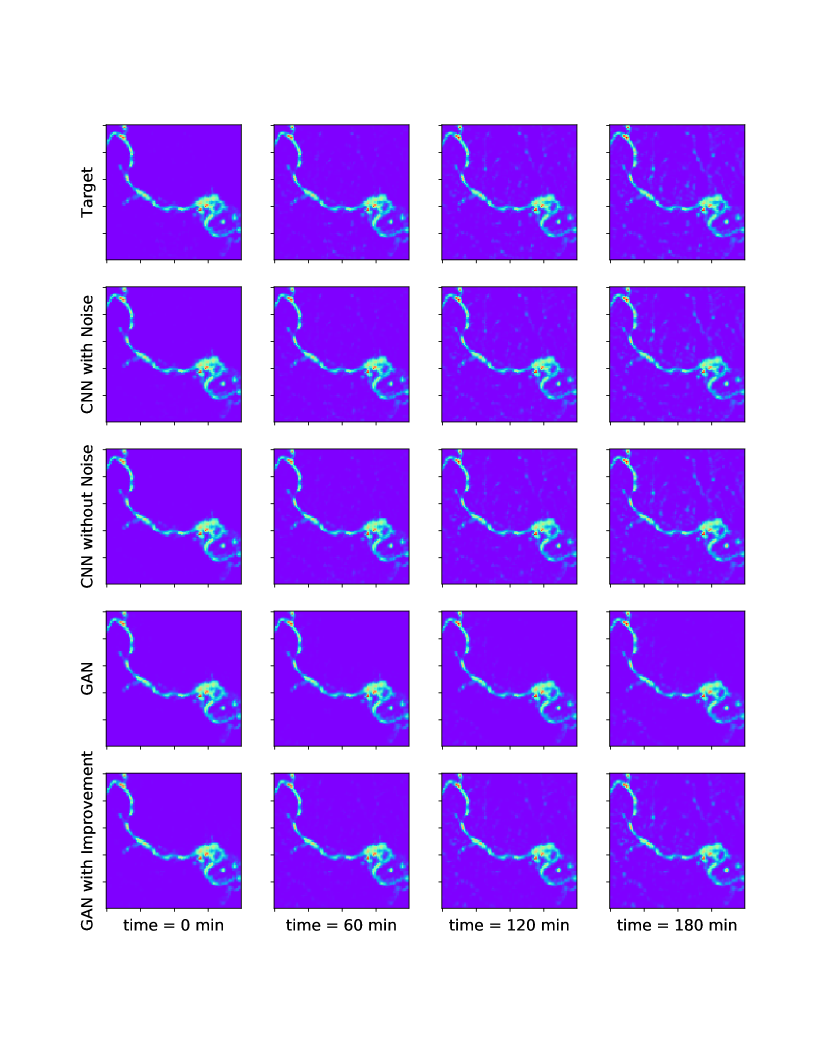
Figure 18: The comparison between targets and different deep learning based prediction methods. We compare the prediction by different methods with targets at $0$ minutes, $60$ minutes, $120$ minutes and $180$ minutes. All the methods are provided with same initial conditions and inputs. The first row is the target.

Figure 19: The comparison between targets and different deep learning based prediction methods. We compare the prediction by different methods with targets at $0$ minutes, $60$ minutes, $120$ minutes and $180$ minutes. All the methods are provided with same initial conditions and inputs. The first row is the target.

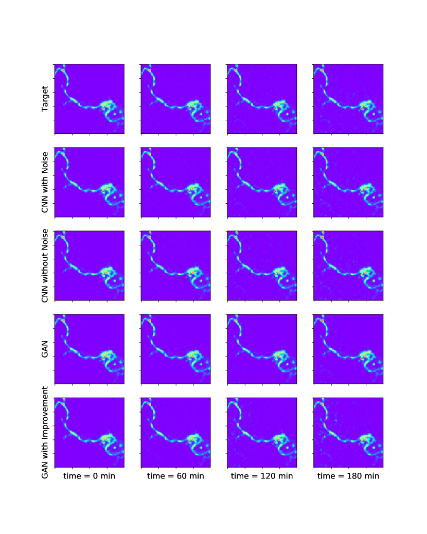
Figure 20: The comparison between targets and different deep learning based prediction methods. We compare the prediction by different methods with targets at $0$ minutes, $60$ minutes, $120$ minutes and $180$ minutes. All the methods are provided with same initial conditions and inputs. The first row is the target.

Figure 21: The comparison between targets and different deep learning based prediction methods. We compare the prediction by different methods with targets at $0$ minutes, $60$ minutes, $120$ minutes and $180$ minutes. All the methods are provided with same initial conditions and inputs. The first row is the target.

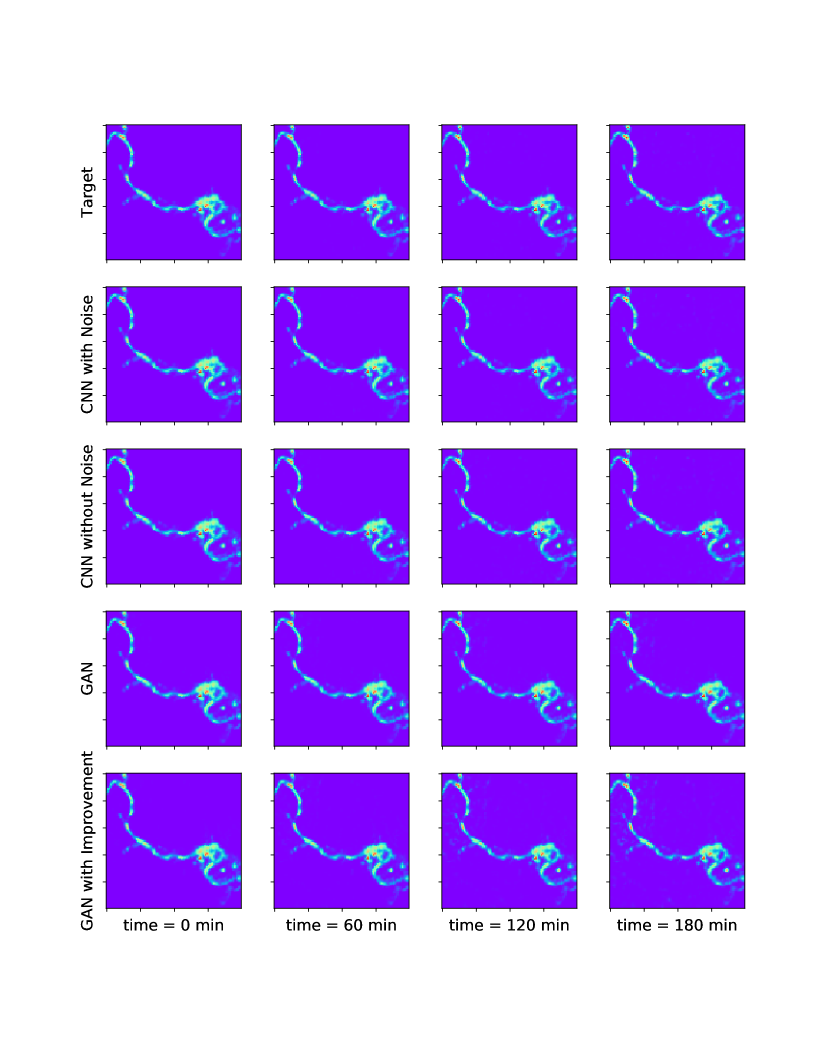
Figure 22: The comparison between targets and different deep learning based prediction methods. We compare the prediction by different methods with targets at $0$ minutes, $60$ minutes, $120$ minutes and $180$ minutes. All the methods are provided with same initial conditions and inputs. The first row is the target.

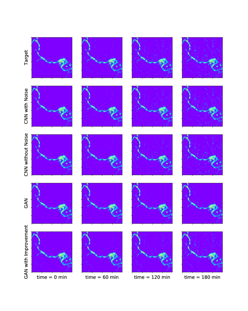
Figure 23: The comparison between targets and different deep learning based prediction methods. We compare the prediction by different methods with targets at $0$ minutes, $60$ minutes, $120$ minutes and $180$ minutes. All the methods are provided with same initial conditions and inputs. The first row is the target.

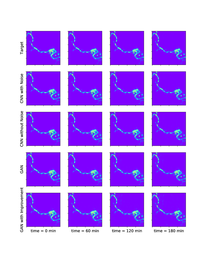
Figure 24: The comparison between targets and different deep learning based prediction methods. We compare the prediction by different methods with targets at $0$ minutes, $60$ minutes, $120$ minutes and $180$ minutes. All the methods are provided with same initial conditions and inputs. The first row is the target.

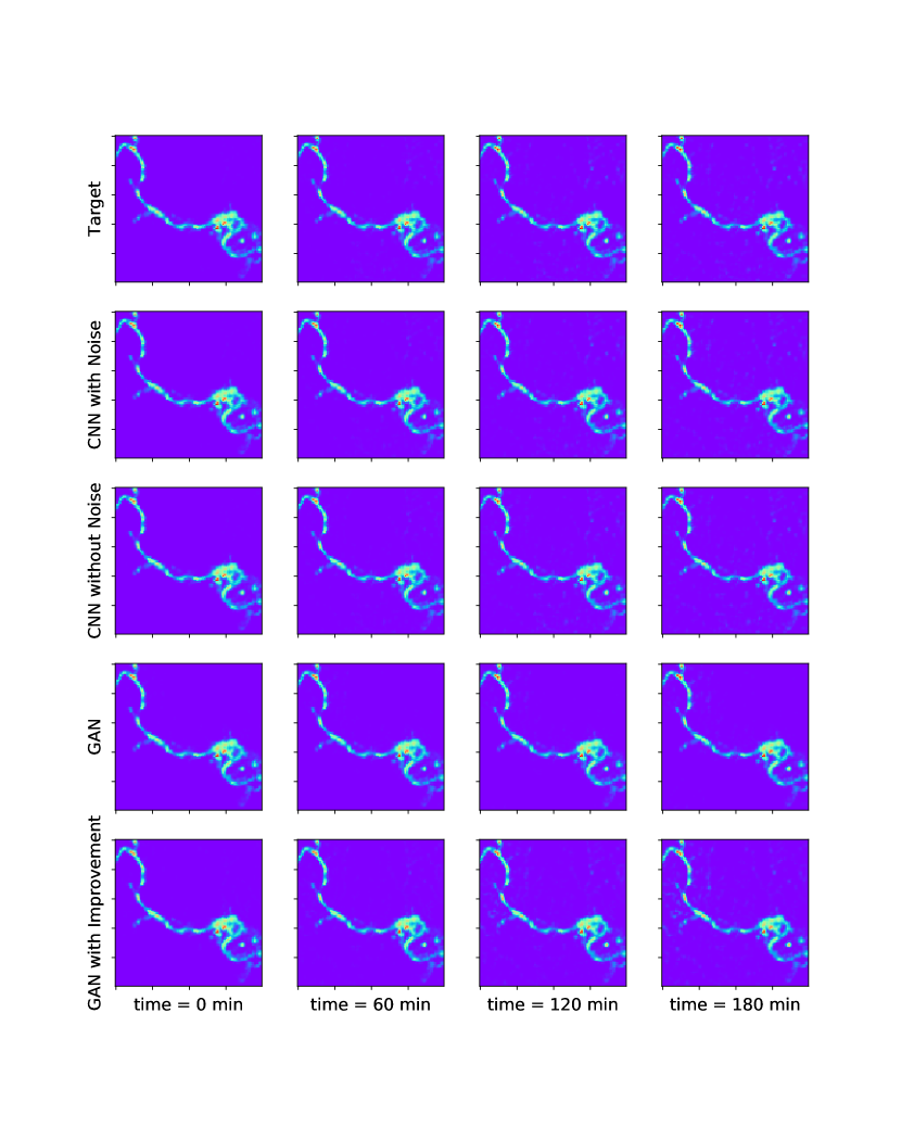
Figure 25: The comparison between targets and different deep learning based prediction methods. We compare the prediction by different methods with targets at $0$ minutes, $60$ minutes, $120$ minutes and $180$ minutes. All the methods are provided with same initial conditions and inputs. The first row is the target.

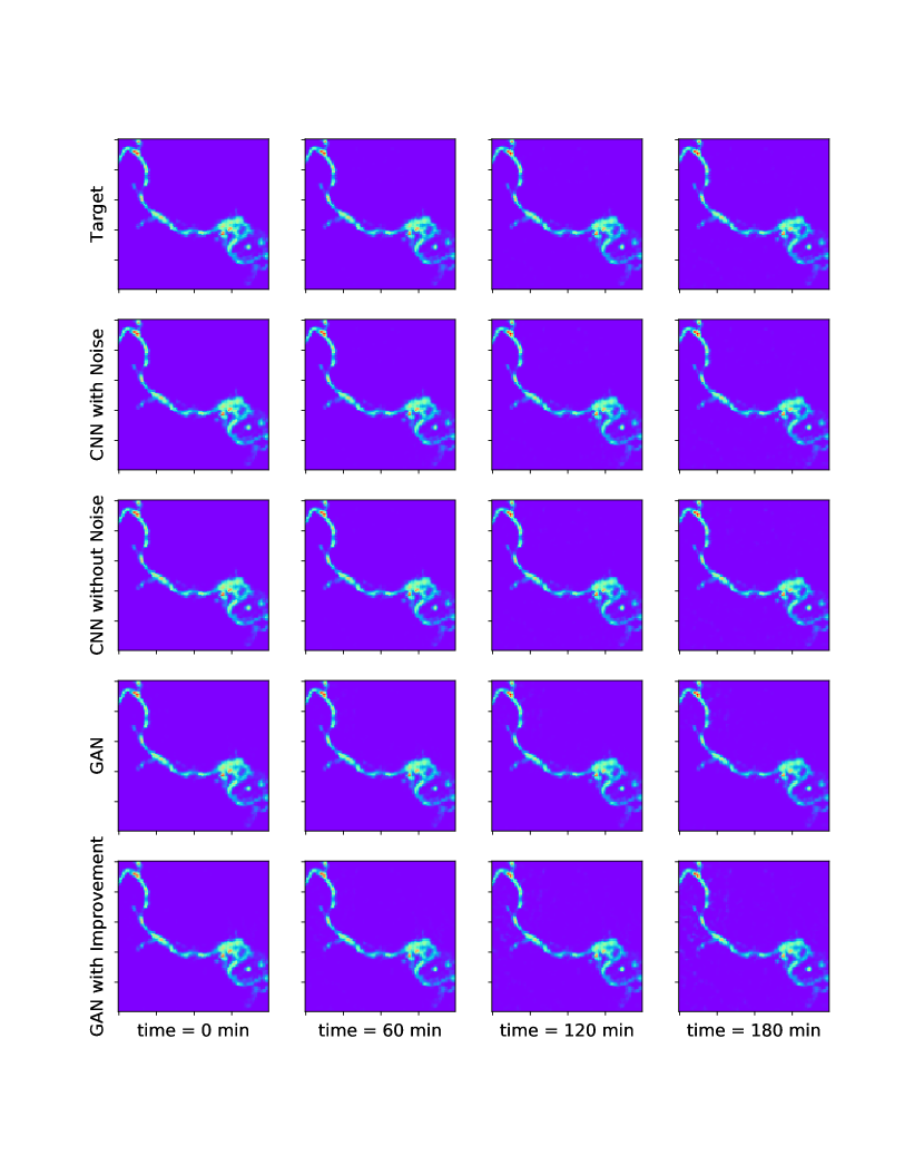
Figure 26: The comparison between targets and different deep learning based prediction methods. We compare the prediction by different methods with targets at $0$ minutes, $60$ minutes, $120$ minutes and $180$ minutes. All the methods are provided with same initial conditions and inputs. The first row is the target.

References

- Alcrudo and Garcia-Navarro (1993) Alcrudo, F., Garcia-Navarro, P., 1993. A high-resolution godunov-type scheme in finite volumes for the 2d shallow-water equations. International Journal for Numerical Methods in Fluids 16 (6), 489–505.
- Alvear et al. (2017) Alvear, O., Zema, N. R., Natalizio, E., Calafate, C. T., 2017. Using uav-based systems to monitor air pollution in areas with poor accessibility. Journal of Advanced Transportation 2017.
- Anastasiou and Chan (1997) Anastasiou, K., Chan, C., 1997. Solution of the 2d shallow water equations using the finite volume method on unstructured triangular meshes. International Journal for Numerical Methods in Fluids 24 (11), 1225–1245.
- Audusse et al. (2004) Audusse, E., Bouchut, F., Bristeau, M.-O., Klein, R., Perthame, B. t., 2004. A fast and stable well-balanced scheme with hydrostatic reconstruction for shallow water flows. SIAM Journal on Scientific Computing 25 (6), 2050–2065.
- Bai et al. (2018) Bai, S., Kolter, J. Z., Koltun, V., 2018. An empirical evaluation of generic convolutional and recurrent networks for sequence modeling. arXiv preprint arXiv:1803.01271.
- Basha et al. (2008) Basha, E. A., Ravela, S., Rus, D., 2008. Model-based monitoring for early warning flood detection. In: Proceedings of the 6th ACM conference on Embedded network sensor systems. ACM, pp. 295–308.
- Bellos and Tsakiris (2016) Bellos, V., Tsakiris, G., 2016. A hybrid method for flood simulation in small catchments combining hydrodynamic and hydrological techniques. Journal of hydrology 540, 331–339.
- Bergman (1999) Bergman, N., 1999. Recursive bayesian estimation: Navigation and tracking applications. Ph.D. thesis, Linköping University.
- Berz (2000) Berz, G., 2000. Flood disasters: lessons from the past—worries for the future. In: Proceedings of the Institution of Civil Engineers-Water and Maritime Engineering. Vol. 142. Thomas Telford Ltd, pp. 3–8.
- Bollermann et al. (2013) Bollermann, A., Chen, G., Kurganov, A., Noelle, S., 2013. A well-balanced reconstruction of wet/dry fronts for the shallow water equations. Journal of Scientific Computing 56 (2), 267–290.
- Bout and Jetten (2018) Bout, B., Jetten, V., 2018. The validity of flow approximations when simulating catchment-integrated flash floods. Journal of hydrology 556, 674–688.
- Brodtkorb et al. (2012) Brodtkorb, A. R., Sætra, M. L., Altinakar, M., 2012. Efficient shallow water simulations on gpus: Implementation, visualization, verification, and validation. Computers & Fluids 55, 1–12.
- Chu and Thuerey (2017) Chu, M., Thuerey, N., 2017. Data-driven synthesis of smoke flows with cnn-based feature descriptors. ACM Transactions on Graphics (TOG) 36 (4), 69.
- Coulibaly et al. (2000) Coulibaly, P., Anctil, F., Bobee, B., 2000. Daily reservoir inflow forecasting using artificial neural networks with stopped training approach. Journal of Hydrology 230 (3-4), 244–257.
- Courant et al. (1928) Courant, R., Friedrichs, K., Lewy, H., 1928. Über die partiellen differenzengleichungen der mathematischen physik. Mathematische annalen 100 (1), 32–74.
- Damle and Yalcin (2007) Damle, C., Yalcin, A., 2007. Flood prediction using time series data mining. Journal of Hydrology 333 (2-4), 305–316.
- Dosovitskiy and Brox (2016) Dosovitskiy, A., Brox, T., 2016. Generating images with perceptual similarity metrics based on deep networks. In: Advances in neural information processing systems. pp. 658–666.
- Dunbabin and Marques (2012) Dunbabin, M., Marques, L., 2012. Robots for environmental monitoring: Significant advancements and applications. IEEE Robotics & Automation Magazine 19 (1), 24–39.
- Elsafi (2014) Elsafi, S. H., 2014. Artificial neural networks (anns) for flood forecasting at dongola station in the river nile, sudan. Alexandria Engineering Journal 53 (3), 655–662.
- Few (2003) Few, R., 2003. Flooding, vulnerability and coping strategies: local responses to a global threat. Progress in Development Studies 3 (1), 43–58.
- Georgakakos (1986) Georgakakos, K. P., 1986. A generalized stochastic hydrometeorological model for flood and flash-flood forecasting: 1. formulation. Water Resources Research 22 (13), 2083–2095.
- Gioia and Bombardelli (2001) Gioia, G., Bombardelli, F., 2001. Scaling and similarity in rough channel flows. Physical review letters 88 (1), 014501.
- Goodfellow et al. (2014) Goodfellow, I., Pouget-Abadie, J., Mirza, M., Xu, B., Warde-Farley, D., Ozair, S., Courville, A., Bengio, Y., 2014. Generative adversarial nets. In: Advances in neural information processing systems. pp. 2672–2680.
- He et al. (2016) He, K., Zhang, X., Ren, S., Sun, J., 2016. Deep residual learning for image recognition. In: Proceedings of the IEEE conference on computer vision and pattern recognition. pp. 770–778.
- Horváth et al. (2015) Horváth, Z., Waser, J., Perdigão, R. A., Konev, A., Blöschl, G., 2015. A two-dimensional numerical scheme of dry/wet fronts for the saint-venant system of shallow water equations. International Journal for Numerical Methods in Fluids 77 (3), 159–182.
- Humphrey et al. (2016) Humphrey, G. B., Gibbs, M. S., Dandy, G. C., Maier, H. R., 2016. A hybrid approach to monthly streamflow forecasting: integrating hydrological model outputs into a bayesian artificial neural network. Journal of Hydrology 540, 623–640.
- Kalman (1960) Kalman, R. E., 1960. A new approach to linear filtering and prediction problems. Journal of basic Engineering 82 (1), 35–45.
- Khac-Tien Nguyen and Hock-Chye Chua (2012) Khac-Tien Nguyen, P., Hock-Chye Chua, L., 2012. The data-driven approach as an operational real-time flood forecasting model. Hydrological Processes 26 (19), 2878–2893.
- Kingma and Ba (2014) Kingma, D. P., Ba, J., 2014. Adam: A method for stochastic optimization. arXiv preprint arXiv:1412.6980.
- Krzhizhanovskaya et al. (2011) Krzhizhanovskaya, V. V., Shirshov, G., Melnikova, N., Belleman, R. G., Rusadi, F., Broekhuijsen, B., Gouldby, B., Lhomme, J., Balis, B., Bubak, M., et al., 2011. Flood early warning system: design, implementation and computational modules. Procedia Computer Science 4, 106–115.
- Kurganov and Levy (2002) Kurganov, A., Levy, D., 2002. Central-upwind schemes for the saint-venant system. ESAIM: Mathematical Modelling and Numerical Analysis 36 (3), 397–425.
- Kurganov et al. (2001) Kurganov, A., Noelle, S., Petrova, G., 2001. Semidiscrete central-upwind schemes for hyperbolic conservation laws and hamilton–jacobi equations. SIAM Journal on Scientific Computing 23 (3), 707–740.
- Kurganov et al. (2007) Kurganov, A., Petrova, G., et al., 2007. A second-order well-balanced positivity preserving central-upwind scheme for the saint-venant system. Communications in Mathematical Sciences 5 (1), 133–160.
- Laio et al. (2003) Laio, F., Porporato, A., Revelli, R., Ridolfi, L., 2003. A comparison of nonlinear flood forecasting methods. Water Resources Research 39 (5).
- LeCun et al. (2015) LeCun, Y., Bengio, Y., Hinton, G., 2015. Deep learning. nature 521 (7553), 436.
- LeCun et al. (1998) LeCun, Y., Bottou, L., Bengio, Y., Haffner, P., et al., 1998. Gradient-based learning applied to document recognition. Proceedings of the IEEE 86 (11), 2278–2324.
- Li and Wand (2016) Li, C., Wand, M., 2016. Combining markov random fields and convolutional neural networks for image synthesis. In: Proceedings of the IEEE Conference on Computer Vision and Pattern Recognition. pp. 2479–2486.
- Liang and Marche (2009) Liang, Q., Marche, F., 2009. Numerical resolution of well-balanced shallow water equations with complex source terms. Advances in water resources 32 (6), 873–884.
- MacQueen et al. (1967) MacQueen, J., et al., 1967. Some methods for classification and analysis of multivariate observations. In: Proceedings of the fifth Berkeley symposium on mathematical statistics and probability. Vol. 1. Oakland, CA, USA, pp. 281–297.
- Mirza and Osindero (2014) Mirza, M., Osindero, S., 2014. Conditional generative adversarial nets. arXiv preprint arXiv:1411.1784.
- Mohammed et al. (2014) Mohammed, F., Idries, A., Mohamed, N., Al-Jaroodi, J., Jawhar, I., 2014. Uavs for smart cities: Opportunities and challenges. In: 2014 International Conference on Unmanned Aircraft Systems (ICUAS). IEEE, pp. 267–273.
- Montz and Gruntfest (2002) Montz, B. E., Gruntfest, E., 2002. Flash flood mitigation: recommendations for research and applications. Global Environmental Change Part B: Environmental Hazards 4 (1), 15–22.
- Moore et al. (1994) Moore, R., Jones, D., Black, K., Austin, R., Carrington, D., Tinnion, M., Akhondi, A., 1994. RFFS and HYRAD: Integrated systems for rainfall and river flow forecasting in real-time and their application in Yorkshire.
- Mosavi et al. (2018) Mosavi, A., Ozturk, P., Chau, K.-w., 2018. Flood prediction using machine learning models: Literature review. Water 10 (11), 1536.
- Raissi (2018) Raissi, M., 2018. Deep hidden physics models: Deep learning of nonlinear partial differential equations. The Journal of Machine Learning Research 19 (1), 932–955.
- Raissi et al. (2017a) Raissi, M., Perdikaris, P., Karniadakis, G. E., 2017a. Physics informed deep learning (part i): Data-driven solutions of nonlinear partial differential equations. arXiv preprint arXiv:1711.10561.
- Raissi et al. (2017b) Raissi, M., Perdikaris, P., Karniadakis, G. E., 2017b. Physics informed deep learning (part ii): Data-driven discovery of nonlinear partial differential equations. arXiv preprint arXiv:1711.10566.
- Roberts et al. (2015) Roberts, S., Nielsen, O., Gray, D., Sexton, J., Davies, G., 05 2015. Anuga user manual, release 2.0.
- Rumelhart et al. (1988) Rumelhart, D. E., Hinton, G. E., Williams, R. J., et al., 1988. Learning representations by back-propagating errors. Cognitive modeling 5 (3), 1.
- Sattari et al. (2012) Sattari, M. T., Yurekli, K., Pal, M., 2012. Performance evaluation of artificial neural network approaches in forecasting reservoir inflow. Applied Mathematical Modelling 36 (6), 2649–2657.
- Shewchuk (1996) Shewchuk, J. R., 1996. Triangle: Engineering a 2d quality mesh generator and delaunay triangulator. In: Workshop on Applied Computational Geometry. Springer, pp. 203–222.
- Sirignano and Spiliopoulos (2018) Sirignano, J., Spiliopoulos, K., 2018. Dgm: A deep learning algorithm for solving partial differential equations. Journal of Computational Physics 375, 1339–1364.
- Sit and Demir (2019) Sit, M., Demir, I., 2019. Decentralized flood forecasting using deep neural networks. arXiv preprint arXiv:1902.02308.
- Tan (1992) Tan, W.-Y., 1992. Shallow water hydrodynamics: Mathematical theory and numerical solution for a two-dimensional system of shallow-water equations. Vol. 55. Elsevier.
- Thuerey et al. (2018) Thuerey, N., Weissenow, K., Mehrotra, H., Mainali, N., Prantl, L., Hu, X., 2018. Well, how accurate is it? a study of deep learning methods for reynolds-averaged navier-stokes simulations. arXiv preprint arXiv:1810.08217.
- Tompson et al. (2017a) Tompson, J., Schlachter, K., Sprechmann, P., Perlin, K., 2017a. Accelerating eulerian fluid simulation with convolutional networks. In: ICML.
- Tompson et al. (2017b) Tompson, J., Schlachter, K., Sprechmann, P., Perlin, K., 2017b. Accelerating eulerian fluid simulation with convolutional networks. In: Proceedings of the 34th International Conference on Machine Learning-Volume 70. JMLR. org, pp. 3424–3433.
- Valipour et al. (2012) Valipour, M., Banihabib, M. E., Behbahani, S. M. R., 2012. Parameters estimate of autoregressive moving average and autoregressive integrated moving average models and compare their ability for inflow forecasting. J Math Stat 8 (3), 330–338.
- Valipour et al. (2013) Valipour, M., Banihabib, M. E., Behbahani, S. M. R., 2013. Comparison of the arma, arima, and the autoregressive artificial neural network models in forecasting the monthly inflow of dez dam reservoir. Journal of hydrology 476, 433–441.
- Vreugdenhil (2013) Vreugdenhil, C. B., 2013. Numerical methods for shallow-water flow. Vol. 13. Springer Science & Business Media.
- Wiewel et al. (2018) Wiewel, S., Becher, M., Thürey, N., 2018. Latent-space physics: Towards learning te temporal evolution of fluid flow. CoRR abs/1802.10123.
- Xie et al. (2018) Xie, Y., Franz, E., Chu, M., Thuerey, N., 2018. tempogan: A temporally coherent, volumetric gan for super-resolution fluid flow. ACM Transactions on Graphics (TOG) 37 (4), 95.
- Xiong et al. (2001) Xiong, L., Shamseldin, A. Y., O’connor, K. M., 2001. A non-linear combination of the forecasts of rainfall-runoff models by the first-order takagi–sugeno fuzzy system. Journal of hydrology 245 (1-4), 196–217.
- Yakowitz (1985) Yakowitz, S., 1985. Markov flow models and the flood warning problem. Water Resources Research 21 (1), 81–88.
- Zoppou and Roberts (1999) Zoppou, C., Roberts, S., 1999. Catastrophic collapse of water supply reservoirs in urban areas. Journal of Hydraulic Engineering 125 (7), 686–695.