Relativistic $k$-fields with Massless Soliton Solutions in $3+1$ Dimensions

Abstract

In this work, the relativistic non-standard Lagrangian densities ($k$-fields) with massless solutions are generally introduced. Such solutions are not necessarily energetically stable. However, in $3+1$ dimensions, we introduce a new $k$-field model that results in a single non-topological massless solitary wave solution. This special solution is energetically stable; that is, any arbitrary deformation above its background leads to an increase in the total energy. In other words, its energy is zero which is the least energy in all solutions. Hence, it can be called a massless soliton solution.

Keywords : $k$-field, soliton, non-standard Lagrangian, massless, zero rest-mass.

1 Introduction

The soliton and solitary wave solutions of the relativistic classical field theory have been a matter of interest in recent decades. They behave like classical particles and properly satisfy the standard relativistic relations [1, 2]. Solitary wave solutions or lumps are special traveling wave solutions with localized energy density functions. A soliton solution is typically defined as a special stable solitary wave solution that reappears after any collision without any distortion [1]. However, in this paper, we only accept the stability condition for defining soliton solutions. Solitary wave solutions are divided into topological and non-topological groups based on their boundary behavior at infinity. Topological solitary wave solutions are inevitably stable, and they are all solitons. The well-known topological kink (anti-kink) solutions of the real nonlinear Klein-Gordon (KG) systems are good examples of the topological solitons in 1+1 dimensions [1, 2, 3, 4, 5, 6]. Also, in $3+1$ dimensions, the solitons of the Skyrme model [2, 7, 8, 9, 10] and magnetic monopole solutions of the ’t Hooft-Polyakov model [1, 2, 11, 12, 13] are the well-known topological solutions of the nonlinear relativistic classical field systems. In general, there is extensive literature on topological solitons, as seen in [14] and the references therein.

In relation to non-topological soliton solutions, most physical models are non-relativistic. For example, the KdV equation or the nonlinear Schrödinger equation are well-known examples of this type. The nonlinear Schrödinger equation and its different variants have been studied extensively in nonlinear optics [15, 16, 17, 18, 19, 20, 21, 22, 23, 24, 25, 26, 27, 28, 29, 30], applied mathematics [31, 32, 33, 34] and plasma [35, 36, 37, 38, 39]. Also, the modified versions of the KdV equation have been of great interest to researchers in applied physics and mathematics [40, 41, 42, 43, 44]. The famous relativistic non-topological solitary wave solutions are Q-balls [45, 46, 47, 48, 49, 50]. Since there is no dependence on the boundaries for the non-topological solitary wave solutions, various criteria have been introduced for the stability considerations. Three stability criteria have been introduced especially for the Q-balls: the classical, the quantum mechanical, and the fission criteria [47, 48, 49, 50, 51]. However, the classical criterion is the most important of all. It is based on dynamical equations obtained for the small fluctuations above the background of the non-topological solitary wave solutions. Above all, if it can be proved that for any arbitrary deformation in the internal structure of a relativistic solitary wave solution, the total energy always increases, it would be an energetically stable solution. The rest energy would be minimal for such a solution compared to other (close) solutions; therefore, the solution would be inevitably stable [52, 53, 54, 55, 56]. For example, the well-known kink (antikinks) solutions are energetically stable entities [1, 52].

All relativistic soliton and solitary wave solutions that have been introduced so far, have non-zero rest-masses. The question is whether it is possible to have a relativistic soliton solution with a zero rest-mass. In general, any particle which moves at the speed of light must be massless. But does any massless particle-like entity have to move at the speed of light? In other words, is it possible to have a zero rest-mass particle-like entity which is at rest or moving at any arbitrary velocity? Mathematically, if we use classical relativistic field theory with soliton solutions, our answer may be slightly different. In [53], it was shown that the existence of a non-moving massless soliton solution can be possible theoretically in $1+1$ dimensions. In this paper, we also show that the existence of the relativistic massless solitons in $3+1$ dimensions are theoretically possible.

To obtain a stable zero rest-mass soliton solution, we need to use a special type of non-standard Lagrangian (NSL) densities for relativistic fields. Briefly, for a set of the real scalar fields $\phi_{j}$ ($j=1,2,\cdots,N$), NSL densities are not linear in the kinetic scalars, which are also called extended KG systems in [53, 54, 55, 56]. The kinetic scalars are different contractions of the scalar fields’ derivatives, i.e. ${\cal S}_{ij}=\partial_{\mu}\phi_{i}\partial^{\mu}\phi_{j}$. The so-called k-fields, fields with dynamics governed by a non-standard kinetic term, is another name for such systems [57, 58, 59]. Historically, the non-standard Lagrangians were first named by Arnold [60] and studied for dynamical systems with a finite number of degrees of freedom, especially in the works of scholars such as Musielak [61, 62, 63] and El-Nabulsi [64, 65, 66, 67, 68]. In this regard, the non-standard exponential Lagrangians (NSELs), non-standard power-law Lagrangians (NSPLs), and non-standard Logarithmic Lagrangians (NSLLs) are three types of NSLs that have received more attention in recent studies [69, 70, 71, 72, 73, 74, 75]. There is a wide range of applications for such systems concerning in differential equations [77, 78, 79, 80, 81], classical and quantum field theory [45, 64, 82, 83, 84, 85, 86, 87, 88, 89, 90, 91, 92, 93], stellar dynamics [94], and plasma waves [95]. In cosmology, the $k$-field models are particularly popular. They are proposed in inflation theory leading to $k$-inflation [86, 87, 88, 89], or used to describe dark energy and dark matter [90, 45, 91, 92, 96]. Classical Yang–Mills field theories with NSL densities can also be used in quantum chromodynamics to explain quark-antiquark interactions at large distances [93].

The organization of this paper is as follows: in the next section, the $k$-field systems with zero rest-mass solutions will be generally introduced. A preliminary $k$-field model will be introduced to illustrate some aspects of the stability of a massless solution. In section 3, a new $k$-field system in $3+1$ dimensions will be introduced that yields to a single massless energetically stable solitary wave solution. The last section is devoted to conclusions.

2 Massless solutions

First of all, let us explain the conditions that must be imposed if we want to have a massless solitary wave solution (defect structure). For a set of relativistic scalar fields $\phi_{k}$ ($k=1,\cdots,N$), the standard Lagrangian densities are functions of the fields and the kinetic scalers ${\cal S}_{ij}=\partial_{\mu}\phi_{i}\partial^{\mu}\phi_{j}$:

$${\cal L}={\cal L}(\phi_{k},{\cal S}_{ij}),\quad\quad(i,j,k=1,\cdots,N)$$ (1)

where $\phi_{k,\mu}=\frac{\partial\phi_{k}}{\partial x^{\mu}}$, and $x^{\mu}\equiv(t,x,y,z)$ . According to the principle of least action, the dynamical equations of motion would be,

$$\frac{\partial{\cal L}}{\partial\phi_{i}}-\frac{\partial}{\partial x^{\mu}}\left(\frac{\partial{\cal L}}{\partial(\partial_{\mu}\phi_{i})}\right)=\frac{\partial{\cal L}}{\partial\phi_{i}}-\sum_{j=1}^{N}\left[\frac{\partial}{\partial x^{\mu}}\left(\frac{\partial{\cal L}}{\partial{\cal S}_{ij}}\right)\partial^{\mu}\phi_{j}+\frac{\partial{\cal L}}{\partial{\cal S}_{ij}}\partial_{\mu}\partial^{\mu}\phi_{j}\right]=0.$$ (2)

In general, since Lagrangian density (1) is invariant under the infinitesimal space-time translations, four continuity equations $\partial_{\mu}T^{\mu\nu}=0$ and then four conserved quantities $P^{\mu}=\int T^{o\mu}d^{3}\textbf{x}$ are obtained, where

$$T^{\mu\nu}=\sum_{i=1}^{N}\frac{\partial{\cal L}}{\partial\phi_{i,\mu}}\frac{\partial\phi_{i}}{\partial x_{\nu}}-{\cal L}g^{\mu\nu},$$ (3)

is called the energy-momentum tensor and $g^{\mu\nu}$ is the $3+1$ dimensional Minkowski metric. The energy density function $\varepsilon$ is the $T^{00}$ component of the energy-momentum tensor (3):

$$T^{00}=\varepsilon=\sum_{i=1}^{N}\frac{\partial{\cal L}}{\partial\dot{\phi}_{i}}\dot{\phi}_{i}-{\cal L}=\sum_{j=1}^{N}\sum_{i=1}^{N}\frac{\partial{\cal L}}{\partial{\cal S}_{ij}}\dot{\phi}_{i}\dot{\phi}_{j}(\delta_{ij}+1)-{\cal L}.$$ (4)

A special localized solution whose energy density function (4) is zero everywhere (i.e. $\varepsilon=0$) can be introduced as a zero rest-mass (massless) solitary wave solution. Also, a zero rest-mass solution clearly has to satisfy dynamical equations (2). Thus, condition $\varepsilon=0$ can be assumed as a new partial differential equation (PDE) along with $N$ coupled PDEs (2). Naturally, the existence of $N+1$ coupled PDEs for $N$ fields is scarcely expected to have a solution. However, if the Lagrangian density and all its derivatives, i.e. ${\cal L}$, $\frac{\partial{\cal L}}{\partial\phi_{i}}$, $\frac{\partial{\cal L}}{\partial{\cal S}_{ij}}$, and $\frac{\partial}{\partial x^{\mu}}(\frac{\partial{\cal L}}{\partial{\cal S}_{ij}})$, become zero for a special solution, these $N+1$ PDEs will no doubt be satisfied automatically and the special solution would be a zero rest-mass solution.

Accordingly, it is easy to understand, based on any standard Lagrangian density $\mathbb{L}$, for which there is a special solution for condition $\mathbb{L}=0$, a new Lagrangian density with a zero rest-mass solution can be introduced as a power of $\mathbb{L}$, i.e. ${\cal L}=\mathbb{L}^{n}$ provided that $n\geqslant 3$. For example, for a single scalar field $\phi$ with a standard nonlinear KG Lagrangian density $\mathbb{L}=\partial_{\mu}\phi\partial^{\mu}\phi+4\phi^{3}-4\phi^{4}$, there is a solution for condition $\mathbb{L}=0$, i.e. $\phi=1/(1+x^{2}+y^{2}+z^{2})$. This solution would be a canonical zero rest-mass solution for a Lagrangian density (${\cal L}=\mathbb{L}^{3}$) as well. In fact, for ${\cal L}=\mathbb{L}^{3}$ we have $\frac{\partial{\cal L}}{\partial\phi}=3\mathbb{L}^{2}\frac{\partial\mathbb{L}}{\partial\phi}$, $\frac{\partial{\cal L}}{\partial{\cal S}}=3\mathbb{L}^{2}\frac{\partial\mathbb{L}}{\partial{\cal S}}$, and $\frac{\partial}{\partial x^{\mu}}(\frac{\partial{\cal L}}{\partial{\cal S}})=6\mathbb{L}\frac{\partial\mathbb{L}}{\partial x^{\mu}}\frac{\partial\mathbb{L}}{\partial{\cal S}}+3\mathbb{L}^{2}\frac{\partial}{\partial x^{\mu}}(\frac{\partial\mathbb{L}}{\partial{\cal S}})$, which are obviously all zero when $\mathbb{L}=0$. In general, for several scalar fields $\phi_{i}$ ($i=1,\cdots,N$), the Lagrangian density of a $k$-field system with a zero rest-mass solution will be introduced as follows:

$${\cal L}=\sum_{n_{1}=0}^{\infty}\sum_{n_{2}=0}^{\infty}\cdots\sum_{n_{m}=0}^{\infty}a({n_{1},\cdots,n_{m}})\mathbb{L}_{1}^{n_{1}}\mathbb{L}_{2}^{n_{2}}\cdots\mathbb{L}_{m}^{n_{m}},$$ (5)

where $\mathbb{L}_{j}$’s ($j=1,\cdots,m$) are a number of independent Lagrangian densities all of which are zero simultaneously for the zero rest-mass solution (i.e., $\mathbb{L}_{j}=0$), provided $n_{1}+n_{2}+\cdots+n_{m}\geqslant 3$. Note that coefficients $a({n_{1},\cdots,n_{m}})$ can be arbitrary functions of the fields and the kinetic scalers ${\cal S}_{ij}$. This form of the Lagrangian densities (5) is very similar to NSPLs introduced by El-Nabulsi for dynamical systems with finite degrees of freedom [68, 69].

So far, we have only explained how the Lagrangian density of a system of fields must yield a massless solution, but we have not considered the stability of such special solutions. The energetical stability condition imposes severe constraints on the Lagrangian density (5), which causes series (5) to be converted to special formats. In fact, no rule has been found yet to develop a system with a single energetically stable massless solitary wave solution, and development of such a system would be mostly based on trial and error. In this section and the next, we will try to show some of the problems of finding a $k$-field system with a single energetically stable zero rest-mass solution.

According to the same $k$-field model in $1+1$ dimensions which was introduced in [53] and led to a single massless solitary wave solution, one can think about the modified version of that in $3+1$ dimensions. In other words, exactly the same Lagrangian density which was introduced in $1+1$ dimensions (Eq. 15 in [53]) for two scalar fields $\phi_{1}=R$ and $\phi_{2}=\theta$ is used here again:

$${\cal L}=\sum_{i=1}^{3}{\cal K}_{i}^{3},$$ (6)

where

$${\cal K}_{1}=R^{2}\mathbb{L}_{2},$$ (7)

$${\cal K}_{2}=R^{2}\mathbb{L}_{2}+\mathbb{L}_{1},$$ (8)

$${\cal K}_{3}=R^{2}\mathbb{L}_{2}+\mathbb{L}_{1}+2R\mathbb{L}_{3},$$ (9)

in which, $\mathbb{L}_{2}={\cal S}_{22}-2$, $\mathbb{L}_{1}={\cal S}_{11}-4R^{4}+4R^{3}$, $\mathbb{L}_{3}={\cal S}_{12}$, ${\cal S}_{11}=\partial_{\mu}R\partial^{\mu}R$, ${\cal S}_{22}=\partial_{\mu}\theta\partial^{\mu}\theta$ and ${\cal S}_{12}=\partial_{\mu}R\partial^{\mu}\theta$.

Now, the main modification is that the kinetic scalars are defined in the $3+1$ dimensions; namely, ${\cal S}_{11}=\partial_{\mu}R\partial^{\mu}R=(\frac{\partial R}{\partial t})^{2}-(\nabla R)^{2}$, and so on. Thus, all the equations of motion and energy density relations (i.e. equations (19)-(26) in [53]) would be obtained again provided one changes $R^{\prime}$ and $\theta^{\prime}$ (i.e. the $x$-derivative of the module and phase field) to $\nabla R$ and $\nabla\theta$, respectively. In [53], it was shown that the existence of a massless solitary wave solution is possible if all ${\cal K}_{i}$’s or $\mathbb{L}_{i}$’s are zero simultaneously. Hence, for ${\cal K}_{i}=0$ ($i=1,2,3$), there was just a unique non-trivial common solitary wave solution as follows:

$$R(x)=\dfrac{1}{1+x^{2}},\quad\quad\theta(t)=\pm\sqrt{2}t.$$ (10)

In the $3+1$ dimensions, the required conditions ${\cal K}_{i}=0$ ($i=1,2,3$) lead to the following covariant PDE’s:

$$\partial_{\mu}\theta\partial^{\mu}\theta=\dot{\theta}^{2}-(\nabla\theta)^{2}=2,$$ (11)

$$\partial_{\mu}R\partial^{\mu}R=\dot{R}^{2}-(\nabla R)^{2}=4R^{4}-4R^{3},$$ (12)

$$\partial_{\mu}R\partial^{\mu}\theta=\dot{\theta}\dot{R}-(\nabla\theta\cdot\nabla R)=0,$$ (13)

where, the dot indicates the time derivative. In general, since there are three independent PDE’s (11)-(13) just for two scalar fields $R$ and $\theta$, mathematically, the existence of the common solutions is severely restricted. However, for the static massless solutions for which $\theta(t)=\sqrt{2}t$ and $R=R(x,y,z)$, PDE’s (11) and (13) are satisfied automatically, and PDE (12) reduced to

$$(\nabla R)^{2}=\left(\frac{\partial R}{\partial x}\right)^{2}+\left(\frac{\partial R}{\partial y}\right)^{2}+\left(\frac{\partial R}{\partial z}\right)^{2}=4R^{3}-4R^{4}.$$ (14)

If we restrict ourselves to the $1+1$ version of model (6) in which $R=R(x)$, the pervious Eq. (14) will be reduced to

$$\left(\frac{dR}{dx}\right)^{2}=4R^{3}-4R^{4},$$ (15)

It is easy to show that nonlinear ordinary differential equation (15) has just a unique non-trivial solution $R=1/(1+x^{2})$, i.e. the one which was introduced in Eq. (10). However, in the $3+1$ version of the model (6), the nonlinear PDE (14) has infinite solutions, such as the following:

$$R(r)=\dfrac{1}{1+(r+\xi)^{2}},$$ (16)

$$R=\frac{1}{1+x^{2}},\quad R=\frac{1}{1+y^{2}},\quad R=\frac{1}{1+z^{2}}$$ (17)

$$R=\frac{1}{1+x^{2}+y^{2}},\quad R=\frac{1}{1+x^{2}+z^{2}},\quad R=\frac{1}{1+y^{2}+z^{2}},$$ (18)

where $r=\sqrt{x^{2}+y^{2}+z^{2}}$ and $\xi$ is any arbitrary real number. According to Eq. (16), for different values of $\xi$, different degenerate massless solutions can be obtained in $3+1$ dimensions. In $1+1$ version of model (6), static solution (16) is reduced to $R=\frac{1}{1+(x+\xi)^{2}}$, but it is nothing more than a space translation in (10) and essentially can not be considered as a new special massless solution. Note that special solutions (17) and (18) are non-localized and cannot be physically interesting.

In [53] or the $1+1$ version of model (6), the main point which guides one to conclude special solitary wave solution (10) is a (massless) soliton solution is the fact that PDE’s (11)-(13) are entirely independent. They have just a unique non-trivial common solitary wave solution (10). Thus, we ensure that Eq. (10) is a single massless solution with the minimum energy of all solutions for the system (6). In other words, for any arbitrary variation above the background of single massless solution (10), the total energy always increases, i.e., it is energetically stable and can be called a soliton solution. But, in the $3+1$ version of model (6), due to the non-existence of a unique non-trivial common solution for PDEs (11)-(13), there is no massless soliton solution. In fact, for PDEs (11)-(13), there is a continuous range of common solutions (16) that are all degenerate massless solutions of the system. Hence, they cannot be called soliton solutions because their profiles can be changed without energy consumption, i.e., there is no stable massless solution. Accordingly, using two scalar fields $R$ and $\theta$ in the $3+1$ version of model (6) does not lead to a unique (massless) common solitary wave solution for three PDE’s (11)-(13). To overcome this problem, the following section will introduce another $k$-field model with three new dynamical fields $\psi_{1}$, $\psi_{2}$ and $\psi_{3}$.

3 A $k$-field system with a single massless soliton solution

For five real scalar fields $\phi_{1}=R$, $\phi_{2}=\theta$, $\phi_{3}=\psi_{1}$, $\phi_{4}=\psi_{2}$ and $\phi_{5}=\psi_{3}$, we can propose a new $k$-field system in the following form:

$${\cal L}=B\sum_{i=1}^{12}{\cal K}_{i}^{3},$$ (19)

where $B$ can be any arbitrary positive number, and

$${\cal K}_{1}=R^{2}\mathbb{L}_{2},\quad~{}~{}~{}{\cal K}_{2}=R^{2}\mathbb{L}_{2}+\mathbb{L}_{1},\quad~{}~{}~{}{\cal K}_{3}=R^{2}\mathbb{L}_{2}+\mathbb{L}_{1}+2R\mathbb{L}_{3},$$

$${\cal K}_{4}=R^{2}\mathbb{L}_{2}+\mathbb{L}_{4},\quad~{}~{}~{}{\cal K}_{5}=R^{2}\mathbb{L}_{2}+\mathbb{L}_{5},\quad~{}~{}~{}{\cal K}_{6}=R^{2}\mathbb{L}_{2}+\mathbb{L}_{6},$$

$${\cal K}_{7}=R^{2}\mathbb{L}_{2}+\mathbb{L}_{4}+\mathbb{L}_{5}+2\mathbb{L}_{7},\quad~{}~{}~{}{\cal K}_{8}=R^{2}\mathbb{L}_{2}+\mathbb{L}_{4}+\mathbb{L}_{6}+2\mathbb{L}_{8},$$

$${\cal K}_{9}=R^{2}\mathbb{L}_{2}+\mathbb{L}_{5}+\mathbb{L}_{6}+2\mathbb{L}_{9},\quad~{}~{}~{}{\cal K}_{10}=R^{2}h_{1}\mathbb{L}_{2}+\mathbb{L}_{1}+\mathbb{L}_{4}+2\mathbb{L}_{10},$$

$${\cal K}_{11}=R^{2}h_{2}\mathbb{L}_{2}+\mathbb{L}_{1}+\mathbb{L}_{5}+2\mathbb{L}_{11},\quad~{}~{}~{}{\cal K}_{12}=R^{2}h_{3}\mathbb{L}_{2}+\mathbb{L}_{1}+\mathbb{L}_{6}+2\mathbb{L}_{12},$$ (20)

in which $h_{j}=[2+\frac{1}{2}(b_{j}-1)^{2}]$, $b_{j}=2\psi_{j}(2R-1)$ ($j=1,2,3$), and

$$\mathbb{L}_{1}={\cal S}_{11}-4R^{4}+4R^{3},\quad~{}~{}~{}\mathbb{L}_{2}={\cal S}_{22}-2,\quad~{}~{}~{}\mathbb{L}_{3}={\cal S}_{12},\quad~{}~{}~{}\mathbb{L}_{4}={\cal S}_{33}+R^{2}-4R^{2}\psi_{1}^{2},$$ (21)

$$\mathbb{L}_{5}={\cal S}_{44}+R^{2}-4R^{2}\psi_{2}^{2},\quad~{}~{}~{}\mathbb{L}_{6}={\cal S}_{55}+R^{2}-4R^{2}\psi_{3}^{2},\quad~{}~{}~{}\mathbb{L}_{7}={\cal S}_{34}-4R^{2}\psi_{1}\psi_{2},$$

$$\mathbb{L}_{8}={\cal S}_{35}-4R^{2}\psi_{1}\psi_{3},\quad~{}~{}~{}\mathbb{L}_{9}={\cal S}_{45}-4R^{2}\psi_{2}\psi_{3},\quad~{}~{}~{}\mathbb{L}_{10}={\cal S}_{13}-b_{1}R^{2},$$

$$\mathbb{L}_{11}={\cal S}_{14}-b_{2}R^{2},\quad~{}~{}~{}\mathbb{L}_{12}={\cal S}_{15}-b_{3}R^{2},$$

where ${\cal S}_{11}=\partial_{\mu}R\partial^{\mu}R$, ${\cal S}_{22}=\partial_{\mu}\theta\partial^{\mu}\theta$, ${\cal S}_{12}=\partial_{\mu}R\partial^{\mu}\theta$, ${\cal S}_{33}=\partial_{\mu}\psi_{1}\partial^{\mu}\psi_{1}$, ${\cal S}_{44}=\partial_{\mu}\psi_{2}\partial^{\mu}\psi_{2}$, ${\cal S}_{55}=\partial_{\mu}\psi_{3}\partial^{\mu}\psi_{3}$, ${\cal S}_{13}=\partial_{\mu}R\partial^{\mu}\psi_{1}$, ${\cal S}_{14}=\partial_{\mu}R\partial^{\mu}\psi_{2}$, ${\cal S}_{15}=\partial_{\mu}R\partial^{\mu}\psi_{3}$, ${\cal S}_{34}=\partial_{\mu}\psi_{1}\partial^{\mu}\psi_{2}$, ${\cal S}_{35}=\partial_{\mu}\psi_{1}\partial^{\mu}\psi_{3}$ and ${\cal S}_{45}=\partial_{\mu}\psi_{2}\partial^{\mu}\psi_{3}$ are some kinetic scalars which are used to introduce the new $k$-field model (19).

Using the Euler-Lagrange equations, one can easily obtain the following dynamical equations:

$$\sum_{i=1}^{12}{\cal K}_{i}\left[2(\partial_{\mu}{\cal K}_{i})\frac{\partial{\cal K}_{i}}{\partial(\partial_{\mu}R)}+{\cal K}_{i}\partial_{\mu}\left(\frac{\partial{\cal K}_{i}}{\partial(\partial_{\mu}R)}\right)-{\cal K}_{i}\frac{\partial{\cal K}_{i}}{\partial R}\right]=0,$$ (22)

$$\sum_{i=1}^{12}{\cal K}_{i}\left[2(\partial_{\mu}{\cal K}_{i})\frac{\partial{\cal K}_{i}}{\partial(\partial_{\mu}\theta)}+{\cal K}_{i}\partial_{\mu}\left(\frac{\partial{\cal K}_{i}}{\partial(\partial_{\mu}\theta)}\right)\right]=0.$$ (23)

$$\sum_{i=1}^{12}{\cal K}_{i}\left[2(\partial_{\mu}{\cal K}_{i})\frac{\partial{\cal K}_{i}}{\partial(\partial_{\mu}\psi_{j})}+{\cal K}_{i}\partial_{\mu}\left(\frac{\partial{\cal K}_{i}}{\partial(\partial_{\mu}\psi_{j})}\right)-{\cal K}_{i}\frac{\partial{\cal K}_{i}}{\partial\psi_{j}}\right]=0,\quad(j=1,2,3).$$ (24)

The sets of functions $R$, $\theta$, and $\psi_{j}$ ($j=1,2,3$) for which ${\cal K}_{i}=0$ ($i=1,\cdots,12$) are simultaneously the special massless solutions of the new $k$-field model (19). Since ${\cal K}_{i}$’s are twelve independent linear combinations of twelve independent scalars $\mathbb{L}_{i}$’s, it is easy to understand that the conditions ${\cal K}_{i}=0$ are equivalent to $\mathbb{L}_{i}=0$ ($i=1,\cdots,12$). The energy-density belonging to the new Lagrangian-density (6) would be

$$\varepsilon(x,t)=T^{00}=\sum_{i=1}^{12}\varepsilon_{i}=B\sum_{i=1}^{12}{\cal K}_{i}^{2}\left[3C_{i}-{\cal K}_{i}\right],$$ (25)

which are divided into twelve distinct parts, in which

$$C_{i}=\dfrac{\partial{\cal K}_{i}}{\partial\dot{\theta}}\dot{\theta}+\dfrac{\partial{\cal K}_{i}}{\partial\dot{R}}\dot{R}+\sum_{j=1}^{3}\dfrac{\partial{\cal K}_{i}}{\partial\dot{\psi_{j}}}\dot{\psi_{j}}=\begin{cases}2R^{2}\dot{\theta}^{2}&\text{i=1}\\ 2(\dot{R}^{2}+R^{2}\dot{\theta}^{2})&\text{i=2}\\ 2(\dot{R}+R\dot{\theta})^{2}&\text{i=3}.\\ 2(\dot{\psi_{1}}^{2}+R^{2}\dot{\theta}^{2})&\text{i=4}.\\ 2(\dot{\psi_{2}}^{2}+R^{2}\dot{\theta}^{2})&\text{i=5}.\\ 2(\dot{\psi_{3}}^{2}+R^{2}\dot{\theta}^{2})&\text{i=6}.\\ 2(\dot{\psi_{1}}+\dot{\psi_{2}})^{2}+2R^{2}\dot{\theta}^{2}&\text{i=7}.\\ 2(\dot{\psi_{1}}+\dot{\psi_{3}})^{2}+2R^{2}\dot{\theta}^{2}&\text{i=8}.\\ 2(\dot{\psi_{2}}+\dot{\psi_{3}})^{2}+2R^{2}\dot{\theta}^{2}&\text{i=9}.\\ 2(\dot{R}+\dot{\psi_{1}})^{2}+2h_{1}R^{2}\dot{\theta}^{2}&\text{i=10}.\\ 2(\dot{R}+\dot{\psi_{2}})^{2}+2h_{2}R^{2}\dot{\theta}^{2}&\text{i=11}.\\ 2(\dot{R}+\dot{\psi_{3}})^{2}+2h_{3}R^{2}\dot{\theta}^{2}&\text{i=12}.\end{cases}$$ (26)

After a straightforward calculation we get:

$$\varepsilon_{1}=B{\cal K}_{1}^{2}[5R^{2}\dot{\theta}^{2}+R^{2}(\nabla\theta)^{2}+2R^{2}],$$ (38)

$$\varepsilon_{2}=B{\cal K}_{2}^{2}[5R^{2}\dot{\theta}^{2}+5\dot{R}^{2}+R^{2}(\nabla\theta)^{2}+(\nabla R)^{2}+U(R)],$$

$$\varepsilon_{3}=B{\cal K}_{3}^{2}[5(R\dot{\theta}+\dot{R})^{2}+(R\nabla\theta+\nabla R)^{2}+U(R)],$$

$$\varepsilon_{4}=B{\cal K}_{4}^{2}[5R^{2}\dot{\theta}^{2}+5\dot{\psi_{1}}^{2}+R^{2}(\nabla\theta)^{2}+(\nabla\psi_{1})^{2}+R^{2}+4R^{2}\psi_{1}^{2}],$$

$$\varepsilon_{5}=B{\cal K}_{4}^{2}[5R^{2}\dot{\theta}^{2}+5\dot{\psi_{2}}^{2}+R^{2}(\nabla\theta)^{2}+(\nabla\psi_{2})^{2}+R^{2}+4R^{2}\psi_{2}^{2}],$$

$$\varepsilon_{6}=B{\cal K}_{6}^{2}[5R^{2}\dot{\theta}^{2}+5\dot{\psi_{3}}^{2}+R^{2}(\nabla\theta)^{2}+(\nabla\psi_{3})^{2}+R^{2}+4R^{2}\psi_{3}^{2}],$$

$$\varepsilon_{7}=B{\cal K}_{7}^{2}[5R^{2}\dot{\theta}^{2}+5(\dot{\psi_{1}}+\dot{\psi_{2}})^{2}+R^{2}(\nabla\theta)^{2}+(\nabla\psi_{1}+\nabla\psi_{2})^{2}+4R^{2}(\psi_{1}+\psi_{2})^{2}],$$

$$\varepsilon_{8}=B{\cal K}_{8}^{2}[5R^{2}\dot{\theta}^{2}+5(\dot{\psi_{1}}+\dot{\psi_{3}})^{2}+R^{2}(\nabla\theta)^{2}+(\nabla\psi_{1}+\nabla\psi_{3})^{2}+4R^{2}(\psi_{1}+\psi_{3})^{2}],$$

$$\varepsilon_{9}=B{\cal K}_{9}^{2}[5R^{2}\dot{\theta}^{2}+5(\dot{\psi_{2}}+\dot{\psi_{3}})^{2}+R^{2}(\nabla\theta)^{2}+(\nabla\psi_{2}+\nabla\psi_{3})^{2}+4R^{2}(\psi_{2}+\psi_{3})^{2}],$$

$$\varepsilon_{10}=B{\cal K}_{10}^{2}[5h_{1}R^{2}\dot{\theta}^{2}+h_{1}R^{2}(\nabla\theta)^{2}+5(\dot{R}+\dot{\psi_{1}})^{2}+(\nabla R+\nabla\psi_{1})^{2}+V(R,\psi_{1})],$$

$$\varepsilon_{11}=B{\cal K}_{11}^{2}[5h_{2}R^{2}\dot{\theta}^{2}+h_{2}R^{2}(\nabla\theta)^{2}+5(\dot{R}+\dot{\psi_{2}})^{2}+(\nabla R+\nabla\psi_{2})^{2}+V(R,\psi_{2})],$$

$$\varepsilon_{12}=B{\cal K}_{12}^{2}[5h_{3}R^{2}\dot{\theta}^{2}+h_{3}R^{2}(\nabla\theta)^{2}+5(\dot{R}+\dot{\psi_{3}})^{2}+(\nabla R+\nabla\psi_{3})^{2}+V(R,\psi_{3})],\quad\quad\quad$$

where

$$U(R)=4R^{4}-4R^{3}+2R^{2},$$ (39)

and

$$V(R,\psi_{j})=U(R)+2R^{2}+R^{2}b_{j}^{2}+4R^{2}\psi_{j}^{2},\quad(j=1,2,3).$$ (40)

Both $U(R)$ and $V(R,\psi_{j})$ are positive definite functions and bounded from below by zero. Thus, all terms in Eqs. (38)-(38) are positive definites and the energy density function (25) is also bounded from below by zero.

As noted before, a special zero rest-mass solution would be possible if $\mathbb{L}_{i}$’s (or equivalently ${\cal K}_{i}$’s) are zero simultaneously. But, mathematically, since there are twelve independent conditions of $\mathbb{L}_{i}=0$ as twelve independent coupled PDE’s for just five scalar fields of $R$, $\theta$ and $\psi_{j}$ ($j=1,2,3$), we normally do not expect them to be satisfied simultaneously. However, we build the new $k$-field system (19) in such a way that there is exceptionally one massless solution for which $\mathbb{L}_{i}=0$ as follows:

$$R=\frac{1}{1+r^{2}},\quad\theta=\pm\sqrt{2}t,\quad\psi_{j}=\pm\frac{x^{j}}{1+r^{2}},\quad(j=1,2,3),$$ (41)

where $x^{1}=x$, $x^{2}=y$ and $x^{3}=z$ (see Fig. 1). Now, unlike the previous model (6) with the undesirable degenerate solutions (16), the following set ($\xi\neq 0$) would not be a special massless solution of the new system (19) anymore:

$$R=\frac{1}{1+(r+\xi)^{2}},\quad\theta=\pm\sqrt{2}t,\quad\psi_{j}=\pm\frac{x^{j}}{1+r^{2}},\quad(\xi\neq 0).$$ (42)

Moreover, one can simply check whether or not the following sets of functions $R$, $\theta$, and $\psi_{j}$ ($j=1,2,3$) are also the special solutions of the new system (19); that is, they are not the common solutions of the PDE’s $\mathbb{L}_{i}=0$ ($i=1,\cdots,12$) simultaneously:

$$R=\frac{1}{1+(r+\xi)^{2}},\quad\theta=\pm\sqrt{2}t,\quad\psi_{j}=\pm\frac{x^{j}}{1+(r+\xi)^{2}},\quad(\xi\neq 0),$$ (43)

$$R=0,\quad\theta=\pm\sqrt{2}t,\quad\psi_{j}=\pm\frac{x^{j}}{1+r^{2}},$$ (44)

$$R=\frac{1}{1+r^{2}},\quad\theta=\pm\sqrt{2}t,\quad\psi_{j}=0,$$ (45)

$$R=\frac{1}{1+x^{2}+y^{2}},\quad\theta=\pm\sqrt{2}t,\quad\psi_{j}=\pm\frac{x^{j}}{1+x^{2}+y^{2}},$$ (46)

$$R=\frac{1}{1+x^{2}},\quad\theta=\pm\sqrt{2}t,\quad\psi_{j}=\pm\frac{x^{j}}{1+x^{2}}.$$ (47)

It should be noted that the new system (19) does not even yield non-localized massless solutions such as Eqs. (46) and (47). The lack of non-localized massless solutions was the main reason why we had to use new scalar fields $\psi_{1}$, $\psi_{2}$, and $\psi_{3}$ to introduce the new system (19). In fact, we did not succeed in finding a simpler system with one or two new scaler fields of $\psi_{1}$ and $\psi_{2}$ without non-localized massless solutions.

Figure 1: The first (second) row is a four dimensional scheme for visualizing $\psi_{1}=x[1+r^{2}]^{-1}$ ($R=[1+r^{2}]^{-1}$).

In general, as in the previous model (6), conditions $\mathbb{L}_{2}=\mathbb{L}_{3}=0$ are satisfied simultaneously for the static solutions (i.e. $R=R(x,y,z)$, $\psi_{j}=\psi_{j}(x,y,z)$, and $\theta=\sqrt{2}t$). The static module function $R(x,y,z)$, however, must participate in $10$ completely different PDE’s as follows:

$$(\nabla R)^{2}=4R^{3}-4R^{4},$$ (48)

$$\nabla\psi_{i}\cdot\nabla\psi_{j}=R^{2}\delta_{ij}-4R^{2}\psi_{i}\psi_{j}\quad(i,j=1,2,3),$$ (49)

$$\nabla\psi_{j}\cdot\nabla R=-2\psi_{j}(2R-1)R^{2},\quad(j=1,2,3).$$ (50)

Since there are ten independent PDE’s (48)-(50) for four static scalar fields $R(x,y,z)$ and $\psi_{j}(x,y,z)$ ($j=1,2,3$), mathematically, the possibility of having a common solution is exceptionally low. More generally, if we do not restrict ourselves to static solutions, there are twelve independent conditions $\mathbb{L}_{i}=0$ only for five real scalar fields $R$, $\theta$, and $\psi_{j}$ ($j=1,2,3$). Thus, it is mathematically very rare to have a common (static or dynamic) solution. In fact, these coupled equations are built deliberately in such a way to make Eq. (41) an exceptional static common solution. In other words, we first consider Eq. (41) and then try to find the proper restrictive conditions $\mathbb{L}_{i}=0$ ($i=1,\cdots,12$) to support it as an outstanding solution. In sum, it seems that the special solution (41) is a single massless solution, and we use this name in the rest of the paper. Suppose one succeeds in finding another massless solution along with (41). In that case, it would be possible to introduce more complicated systems by imposing new scalar fields with additional restrictive conditions $\mathbb{L}_{i}=0$ to ensure the uniqueness of a massless solitary wave solution.

Since the Lagrangian density (19) is essentially Poincaré invariant, any rotation of non-spherical symmetric functions $\psi_{j}=\pm x^{j}(1+r^{2})^{-1}$ ($j=1,2,3$) can be used equivalently in Eq. (41). For example, instead of $\psi_{j}=\pm x^{j}(1+r^{2})^{-1}$ ($j=1,2,3$) in Eq. (41), we can use $\psi_{1}=\pm(\cos(\alpha)x+\sin(\alpha)y)(1+r^{2})^{-1}$, $\psi_{2}=\pm(-\sin(\alpha)x+\cos(\alpha)y)(1+r^{2})^{-1}$ and $\psi_{3}=\pm z(1+r^{2})^{-1}$ (i.e. any arbitrary rotation about $z$-axis), where $\alpha$ is any arbitrary angle. However, since all different spatial rotations are physically equivalent, we can just consider the same simple functions $\psi_{j}=\pm x^{j}(1+r^{2})^{-1}$ ($j=1,2,3$) as the proper candidates for all of them.

According to Eqs. (38)-(38), since all terms in energy density functional (25) are positive definites, this property imposes a strong condition to ensure that the single massless solution (41) is really an energetically stable object or a soliton solution, which means that any arbitrary deformation above the background of that leads to an increase in the total energy. Any arbitrary small deformed version of special solution (41) can be introduced as follows:

$$R=(1+r^{2})^{-1}+\delta R,\quad\theta=\sqrt{2}t+\delta\theta,\quad\psi_{j}=\pm x^{j}(1+r^{2})^{-1}+\delta\psi_{j},\quad(j=1,2,3)$$ (51)

where $\delta R$, $\delta\theta$, and $\delta\psi_{j}$ (small variations) are considered to be any arbitrary small functions of space-time. If we insert (51) into $\varepsilon_{i}$ ($i=1,\cdots,12$), we find

$$\delta\varepsilon_{i}=B[3(C_{i}+\delta C_{i})({\cal K}_{i}+\delta{\cal K}_{i})^{2}-({\cal K}_{i}+\delta{\cal K}_{i})^{3}]=B[3(C_{i}+\delta C_{i})(\delta{\cal K}_{i})^{2}-(\delta{\cal K}_{i})^{3}]\approx$$

$$\quad\quad B[3C_{i}(\delta{\cal K}_{i})^{2}-(\delta{\cal K}_{i})^{3}]\approx[3BC_{i}(\delta{\cal K}_{i})^{2}]>0.\quad\quad$$ (52)

Note that, for massless solution (41), ${\cal K}_{i}=0$ and $\varepsilon_{i}=0$ ($i=1,\cdots,12$). Hence, since $C_{i}>0$, according to Eq. (3), $\delta\varepsilon_{i}$ ($i=1,\cdots,12$) and $\delta E=\int\sum_{i=1}^{12}\delta\varepsilon_{i}d^{3}x$ have always positive definite values for all small variations; that is, massless solution (41) is energetically stable. In other words, for any arbitrary deformation above the background of special solution (41), at least one of the ${\cal K}_{i}$’s (or equivalently one of the $\varepsilon_{i}$’s) would be a non-zero functional. It leads to the non-zero positive energy density functionals (3), and then the total energy variation $\delta E$ will be always larger than zero. Since special massless solution (41) is single, other solutions of the dynamical equations (22)-(24) can be considered as the small or large deformations of that. Hence, they all have non-zero positive rest energies; that is to say, special solution (41) has always the minimum energy of all. To summarize, based on the very strict conditions that have been set, special massless solution (41) is single and stable against any arbitrary deformation. Hence, there is no possibility that this particle-like entity (41) with zero energy will decay and turn into radiations.

For more support, let us consider the total energy variation ($E=\delta E$) for many arbitrary small deformations above the background of special massless solution (41) numerically. For example, a number of arbitrary ad hoc deformations can be the same as the one introduced in Eq. (43) and eleven other cases as follows:

$$R=(1+\xi)(1+r^{2})^{-1},\quad\theta=\pm\sqrt{2}t,\quad\psi_{j}=\pm x^{j}(1+r^{2})^{-1},$$ (53)

$$R=(1+r^{2})^{-1},\quad\theta=\pm\sqrt{2}t,\quad\psi_{j}=\pm(1+\xi)x^{j}(1+r^{2})^{-1},$$ (54)

$$R=(1+(r+\xi)^{2})^{-1},\quad\theta=\pm\sqrt{2}t,\quad\psi_{j}=\pm x^{j}(1+r^{2})^{-1},$$ (55)

$$R=(1+\xi+r^{2})^{-1},\quad\theta=\pm\sqrt{2}t,\quad\psi_{j}=\pm x^{j}(1+r^{2})^{-1},$$ (56)

$$R=(1+r^{2})^{-1},\quad\theta=\pm\sqrt{2}t,\quad\psi_{j}=\pm x^{j}(1+\xi+r^{2})^{-1},$$ (57)

$$R=(1+r^{2})^{-1},\quad\theta=\pm(\sqrt{2}+\xi)t,\quad\psi_{j}=\pm x^{j}(1+r^{2})^{-1},$$ (58)

$$R=(1+r^{2})^{-1}+\xi e^{-r^{2}},\quad\theta=\pm\sqrt{2}t,\quad\psi_{j}=\pm x^{j}(1+r^{2})^{-1},$$ (59)

$$R=(1+r^{2})^{-1},\quad\theta=\pm\sqrt{2}t,\quad\psi_{j}=\pm(x^{j}+\xi)(1+r^{2})^{-1},$$ (60)

$$R=(1+r^{2})^{-1},\quad\theta=\pm\sqrt{2}t,\quad\psi_{j}=\pm x^{j}(1+(r+\xi)^{2})^{-1},$$ (61)

$$R=(1+(1+\xi)x^{2}+y^{2}+z^{2})^{-1},\quad\theta=\pm\sqrt{2}t,\quad\psi_{j}=\pm x^{j}(1+r^{2})^{-1},$$ (62)

$$R=(1+r^{2})^{-1},\quad\theta=\pm\sqrt{2}t,\quad\psi_{1}=\pm(x+\xi)(1+r^{2})^{-1},$$

$$\quad\quad\psi_{2}=\pm y(1+r^{2})^{-1},\quad\psi_{3}=\pm z(1+r^{2})^{-1},$$ (63)

where $\xi$ is a small parameter whose larger values correspond to larger deformations. The case $\xi=0$ leads to the same special massless solution (41). For such arbitrary deformations (43) and (53)-(63) at $t=0$, Fig. 2 demonstrates that a larger deformation leads to a further increase in the total energy, as expected. Furthermore, it is obvious that parameter $B$ has a main role in the stability of special massless solution (41), and its larger values lead to higher stability (of the special solution). To put it differently, the larger the values, the greater the increase in the total energy for any arbitrary small variation above the background of special massless solution (41).

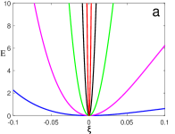
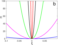
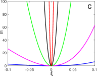
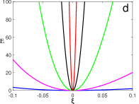
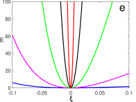
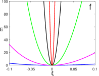
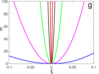
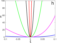
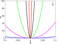
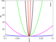
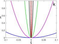
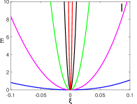
Figure 2: Plots a-l represent variations of the total energy $E$ versus small $\xi$ for different deformations (43) and (53)-(63) at $t=0$, respectively. Various color curves of blue, purple, green, black, and red are related to $B=1$, $B=10$, $B=100$, $B=1000$, and $B=10000$, respectively.

Since the theory is relativistic, the moving version of single massless solitary wave solution (41) can be easily obtained. Hence, a moving solution along the $x$-axis is given by

$$R=\frac{1}{1+\gamma^{2}(x-vt)^{2}+y^{2}+z^{2}},\quad\theta=k_{\mu}x^{\mu},\quad\psi_{1}=\pm\frac{\gamma(x-vt)}{1+\gamma^{2}(x-vt)^{2}+y^{2}+z^{2}},$$

$$\psi_{2}=\pm\frac{y}{1+\gamma^{2}(x-vt)^{2}+y^{2}+z^{2}},\quad\psi_{3}=\pm\frac{z}{1+\gamma^{2}(x-vt)^{2}+y^{2}+z^{2}},$$ (64)

where $k^{\mu}\equiv(\gamma\omega_{s},\gamma\omega_{s}v,0,0)$. Since the model is relativistic, the total energy of moving version (3) of the special solution (41) is also zero. In fact, for moving version (3), as well as the static version (41), all independent scalars $\mathbb{L}_{i}$ and ${\cal K}_{i}$ ($i=1,\cdots,12$) would be zero simultaneously. Thus, according to Eqs. (38)-(38), the energy density function and subsequently the total energy, irrespective of the velocity, are zero. However, based on all previous knowledge of numerical simulations about field evolutions in interactions, we can claim that having a rigid entity without any small deformation is generally impossible. In fact, the internal structure of any solitary wave solution would be slightly deformed in the interactions. Therefore, for special massless solution (41), the rest-mass (energy) is never absolutely zero. In other words, the variations of the fields $\delta R$, $\delta\psi_{j}$ ($j=1,2,3$), and $\delta\theta$ do not remain zero in the interactions; hence, $\delta{\cal K}_{i}$, $\delta\varepsilon_{i}$ ($i=1,\cdots,12$), and total energy are not absolute zero. Accordingly, it is not really a rigid entity with absolute zero rest-mass; therefore, the effect of any interaction may cause its speed to approach the speed of light, but not exactly reach it.

Since special solution (41) is non-topological, a multi particle-like (lump) solution can be easily obtained only by adding any arbitrary number of the distant (moving) special solutions (41) together. In fact, the non-topological solutions are zero at far distances, hence, when they are too far apart, the tail of each non-topological solution would be zero in the positions of other solutions. In other words, the effect of each non-topological solution on the others is practically zero when they are too far apart, similar to many point charges which stand at far distances from one another. For example, we can consider two moving special solutions (41) which initially stand at different positions $(a,0,0)$ and $(b,0,0)$, and have different velocities $\textbf{v}_{1}=-\textbf{v}_{2}=v\widehat{i}$ along the $x$-axis. If $|b-a|$ is large enough, their linear combination, i.e.

$$R=\frac{1}{1+\gamma^{2}(x-vt-a)^{2}+y^{2}+z^{2}}+\frac{1}{1+\gamma^{2}(x+vt-b)^{2}+y^{2}+z^{2}}$$

$$\psi_{1}=\frac{\gamma(x-vt-a)}{1+\gamma^{2}(x-vt-a)^{2}+y^{2}+z^{2}}+\frac{\gamma(x+vt-b)}{1+\gamma^{2}(x+vt-b)^{2}+y^{2}+z^{2}},$$

$$\psi_{j}=\frac{x^{j}}{1+\gamma^{2}(x-vt-a)^{2}+y^{2}+z^{2}}+\frac{x^{j}}{1+\gamma^{2}(x+vt-b)^{2}+y^{2}+z^{2}}\quad\quad(j=2,3),$$

is again a solution at the initial times (i.e. the times that are close to $t=0$). For such a linear combination, it is observed numerically that the terms $\mathbb{L}_{i}$ ($i=1,\cdots,12$) are all approximately zero. Hence, based on dynamical equations (22)-(24), such a linear combination would be an approximate solution again. The greater the distance between the two special solutions, the more accurate this approximation will be. It should be noted that for such a linear combination, the velocity-dependent phase-field $\theta$ changes from $\theta_{1}=k_{1\mu}x^{\mu}$ ($k_{1\mu}k_{1}^{\mu}=2$) at the position of the first special solution to $\theta_{2}=k_{2\mu}x^{\mu}$ ($k_{2\mu}k_{2}^{\mu}=2$) at the position of the second one. In fact, in the free space between two special solutions, where scalar fields $R$, $\psi_{j}$ ($j=1,2,3$), and $\varepsilon$ are all almost zero, there is no rigorous condition on the phase-field to be a solution of $\mathbb{L}_{2}=0$.

4 Conclusions

For several scalar fields $\phi_{i}$ ($i=1,\cdots,N$), we reintroduced the relativistic $k$-fields systems as non-standard Lagrangian densities which are not linear in the kinetic scalars ${\cal S}_{ij}=\partial_{\mu}\phi_{i}\partial^{\mu}\phi_{j}$. For a group of these systems, we showed that it is possible to have zero rest-mass solutions whose energy density functions are zero. These massless solutions are not necessarily energetically stable, and finding a stable case is not simple. Expecting this stable solution to be a non-topological entity would increase the difficulty of this goal. However, we introduced a $k$-field system (19) in the $3+1$ dimensions which leads to a single massless non-topological energetically stable soliton solution (41).

Model (19) is based on introducing twelve independent scalar functionals ${\cal K}_{i}$’s ($i=1,\cdots,12$) of five scalar fields $R$, $\theta$ and $\psi_{j}$ ($j=1,2,3$). In general, all terms in the related dynamical equations (22)-(24) contain the first or second power of one of the ${\cal K}_{i}$’s. Also, all terms in the energy density function are positive definites and all contain the square of one of the twelve independent functionals ${\cal K}_{i}$’s. Thus, the solutions for which all ${\cal K}_{i}$’s equal zero simultaneously are special massless solutions. Nevertheless, the simultaneous satisfaction of twelve independent conditions ${\cal K}_{i}=0$ for five scalar fields is not mathematically possible. However, we built this model in such a way that there is an exceptional massless solution (41) for which ${\cal K}_{i}=0$ ($i=1,\cdots,12$).

In general, if there is a rigid massless entity, the effect of any small force changes its speed to approach the speed of light immediately. However, if we assume particles as the soliton solutions of the nonlinear field theories, the existence of a rigid particle would not be possible normally. In other words, they would be deformed in any interaction, no matter how small. Hence, hypothetical massless particles can never exactly reach the speed of light. If they exist, they are affected by the environment and their energies would not be absolute zero.

Since special massless solution (41) is single, and since all terms in the energy density function (see Eqs. (38)-(38)) are positive definites, the energetical stability of special massless solution (41) is guaranteed properly; which means that, for any arbitrary deformation above the background, the total energy increases. In other words, the other solutions of system (6) for which at least one of the ${\cal K}_{i}$’s is a non-zero functional have non-zero positive total energies. Thus, the energy of the single massless solution (41) would be the least of all solutions. Accordingly, we can call special solution (41) a (massless) soliton solution. To summarize, this model shows that the relativistic classical field theory can lead to stable particle-like solutions with zero rest-masses in $3+1$ dimensions.

References

• [1] R. Rajaraman Solitons and instantons (Amsterdam North Holland, Elsevier) (1982).
• [2] N. Manton P Sutcliffe Topological solitons (Cambridge University Press) (2004).
• [3] A A Izquierdo, J Queiroga-Nunes and L M Nieto Physical Review D 103 045003 (2021).
• [4] M Mohammadi and R Dehghani Communications in Nonlinear Science and Numerical Simulation 94 105575 (2021).
• [5] D Bazeia, A R Gomes and F C Simas The European Physical Journal C 81 1 (2021).
• [6] V A Gani, V Lensky and M A Lizunova Journal of High Energy Physics 2015 147 (2015).
• [7] T H R Skyrme Proceedings of the Royal Society A. 260 127 (1961).
• [8] T H R Skyrme Nuclear Physics, 31 556 (1962).
• [9] N S Manton, B J Schroers and M A Singer Communications in mathematical physics 245 123 (2004).
• [10] O L Battistel Brazilian journal of physics 34 742 (2004).
• [11] G โ€™t Hooft Nuclear Physics B 79 276 (1974).
• [12] A M Polyakov JETP Letters 20 430 (1974).
• [13] S Nishino, R Matsudo, M Warschinke and K I ondo Progress of Theoretical and Experimental Physics 2018 103B04 (2018).
• [14] M Eto, Y Hirono, Nitta and S Yasui Progress of Theoretical and Experimental Physics, 2014 012D01 (2014).
• [15] A R Seadawy and D Lu Physical Review E 94 823 (2020).
• [16] Z Korpinar, M Inc, B Almohsen and M Bayram Indian Journal of Physics 95 2143 (2021).
• [17] H Sakaguchi and B A Malomed Physical Review E 72 046610 (2005).
• [18] M Mirzazadeh, M Eslami and A H Arnous European Physical Journal Plus 130 1 (2015).
• [19] M Younis, S T R Rizvi Journal of nanoelectronics and optoelectronics 10 179 (2015).
• [20] E C Aslan and M Inc Optik 196 162661 (2019).
• [21] W X Ma and M Chen Applied Mathematics and Computation 215 2835 (2009).
• [22] M Savescu, K R Khan, P Naruka, H Jafari, L Moraru and A Biswas Journal of Computational and Theoretical Nanoscience 10 1182 (2013).
• [23] X Liu, H. Zhang and W Liu, Applied Mathematical Modelling 102 305 (2022).
• [24] G Ma, J Zhao, Q Zhou, A Biswas and L Liu Nonlinear Dynamics 106 2479 (2021).
• [25] L L Wang and W J Liu Chinese Physics B 29 070502 (2020).
• [26] Y Y Yan and W J Liu Chinese Physics Letters 38 094201 (2021).
• [27] L Wang, Z Luan, Q Zhou, A Biswas A K Alzahrani and W Liu Nonlinear dynamics 104 2613 (2021).
• [28] H Wang, Q Zhou, A Biswas and W Liu Nonlinear Dynamics 106 841 (2021).
• [29] G Ma, Q Zhou, W Yu, A Biswas and W Liu Nonlinear Dynamics 2509 106 (2021).
• [30] T Y Wang, Q Zhou and W J Liu Chinese Physics B 31 020501 (2022).
• [31] A M Wazwaz Chaos, Solitons $\&$ Fractals 37 1136 (2008).
• [32] Y Zhou, M Wang and T Miao Physics Letters A 323 77 (2004).
• [33] N Mahak and G Akram The European Physical Journal Plus 134 1 (2019).
• [34] M M El-Borai, H M El-Owaidy, H M Ahmed and A H Arnous Nonlinear Science Letters A 8 32 (2017).
• [35] K M Li Indian Journal of Physics 88 93 (2014).
• [36] J Akter, N A Chowdhury, A Mannan and A A Mamun Indian Journal of Physics 1 (2021).
• [37] S A El-Tantawy, S A Shan, N Akhtar and A T Elgendy Chaos, Solitons $\&$ Fractals 113 356 (2018).
• [38] M S Ruderman, T Talipova and E Pelinovsky Journal of Plasma Physics 74 639 (2008).
• [39] P Eslami and M Mottaghizadeh Indian Journal of Physics 88, 521 (2014).
• [40] G Rowlands, P Rozmej, E Infeld and A Karczewska The European Physical Journal E 49 1 (2017).
• [41] M K Brun and H Kalisch Analysis and Mathematical Physics 8 57 (2018).
• [42] Z Emami and H R Pakzad Indian Journal of Physics, 85 1643 (2011).
• [43] M Wang Physics Letters A 213 (1996).
• [44] H X Ge, R J Cheng and S Q Dai Physica A: Statistical Mechanics and its Applications 357 466 (2005).
• [45] D Bazeia, L Losano, M A Marques and R Menezes Physics Letters B 765 359 (2017).
• [46] D Bazeia, L Losano, M A Marques, R Menezes and R da Rocha Physics Letters B 758 146 (2016).
• [47] A G Panin and M NmSmolyakov Physical Review D 95 065006 (2017).
• [48] A Kovtun, E Nugaev and A Shkerin Physical Review D 98 096016 (2018).
• [49] M N Smolyakov Physical Review D 97 045011 (2018).
• [50] M I Tsumagari, E J Copeland and P M Saffin Physical Review D 78 065021 (2008).
• [51] M N Smolyakov Physical Review D 100 045002 (2019).
• [52] G H Derrick Journal of Mathematical Physics 5 1252 (1964).
• [53] M Mohammadi and R Gheisari Physica Scripta 95 015301 (2019).
• [54] M Mohammadi Annals of Physics 414 168099 (2020).
• [55] M Mohammadi Physica Scripta 95 045302 (2020).
• [56] M Mohammadi Annals of Physics 422 168304 (2020).
• [57] D Bazeia, L Losano, R Menezes and J C R E Oliveira The European Physical Journal C 51 953 (2007).
• [58] C Adam, J Sanchez-Guillen and A Wereszczyล„ski Journal of Physics A: Mathematical and Theoretical 40 13625 (2007).
• [59] E Babichev Physical Review D 74 085004 (2006).
• [60] V I Arnold, Mathematical Methods of Classical Mechanics, Springer, New York, (1978).
• [61] Z E Musielak Journal of Physics A: Mathematical and Theoretical 41 055205 (2008).
• [62] Z E Musielak, D Roy and L D Swift Chaos, Solitons $\&$ Fractals 38 894 (2008).
• [63] Z E Musielak Chaos, Solitons $\&$ Fractals 42 2645 (2009).
• [64] A R El-Nabulsi Indian Journal of Physics 87 379 (2013).
• [65] R A El-Nabulsi Nonlinear Dynamics 74 381 (2013).
• [66] R A El-Nabulsi Nonlinear Dynamics 79 2055 (2015).
• [67] R A El-Nabulsi Proceedings of the National Academy of Sciences, India Section A: Physical Sciences 85 247 (2015).
• [68] R A El-Nabuls Qualitative theory of dynamical systems 12 273 (2013).
• [69] R A El-Nabulsi Applied Mathematics Letters 43 120 (2015).
• [70] J Song and Y Zhang Acta Mechanica 229 285 (2018).
• [71] Y Zhou and X S Zhou Nonlinear Dynamics 84 1867 (2016).
• [72] J F Cari$\tilde{\textrm{n}}$ena and J Fern$\acute{\textrm{a}}$ndez N$\acute{\textrm{u}}$ $\tilde{\textrm{n}}$ez Nonlinear Dynamics 83 457 (2016).
• [73] J F Cari$\tilde{\textrm{n}}$ena and J Fern$\acute{\textrm{a}}$ndez N$\acute{\textrm{a}}$ $\tilde{\textrm{n}}$ez Nonlinear Dynamics 86 1285 (2016).
• [74] R A El-Nabulsi Tbilisi Mathematical Journal 9 279 (2016).
• [75] A R El-Nabulsi Mathematical Sciences 9 173 (2015).
• [76] Y Zhang and X P Wang Symmetry 11 1061 (2019).
• [77] N A Kudryashov and D I Sinelshchikov Applied Mathematics Letters 63 124 (2017).
• [78] J F Cari$\tilde{\textrm{n}}$ena and P Guha International Journal of Geometric Methods in Modern Physics 16 1940001 (2019).
• [79] J F Carinena, M F Ranada and M Santander Journal of mathematical physics 46 062703 (2005).
• [80] V K Chandrasekar, S N Senthilvelan and M Lakshmanan Journal of mathematical physics 47 023508 (2006).
• [81] A Saha and B Talukdar Talukdar Reports on Mathematical Physics 73 299 (2014).
• [82] R A El-Nabulsi Indian Journal of Physics 87 379 (2013).
• [83] R A El-Nabulsi 83 Proceedings of the National Academy of Sciences, India Section A: Physical Sciences 383 (2013).
• [84] R A El-Nabulsi Indian Journal of Physics 87 465 (2013).
• [85] R A El-Nabulsi Zeitschrift FF$\ddot{\textrm{u}}$r Naturforschung 71 817 (2016).
• [86] C Armend$\acute{\textrm{a}}$riz-Pic$\acute{\textrm{o}}$n, T Damour and V I Mukhanov Physics Letters B 458 209 (1999).
• [87] T Chiba, T Okabeand M Yamaguchi Physical Review D 62 023511 (2000).
• [88] C Armendariz-Picon, V Mukhanov and P J Steinhardt Physical Review Letters 85 4438 (2000).
• [89] R A El-Nabulsi Journal of the Korean Physical Society 79 345 (2021).
• [90] C Armendariz-Picon and E A Lim Journal of Cosmology and Astroparticle Physics 2005 007 (2005).
• [91] T Padmanabhan and T R Choudhury Physical Review D 66 081301 (2002).
• [92] S Renaux-Petel and G Tasinato Journal of Cosmology and Astroparticle Physics 2009 012 (2009).
• [93] A I Alekseev and B A Arbuzov Theoretical and Mathematical Physics 59 372 (1984).
• [94] R A El-Nabulsi Communications in Theoretical Physics 69 233 (2018).
• [95] R A El-Nabulsi Proceedings of the Royal Society A 476 20200190 (2020).
• [96] R A El-Nabulsi Journal of Theoretical and Applied Physics 7 58 (2013).
• [97] A R El-Nabulsi Canadian Journal of Physics 92 1149 (2014).